1. Introduction
Reliability analysis plays a critical role in understanding the lifespan and performance of systems and components in various fields, such as engineering, medicine, and industrial applications. Among the statistical models used for lifetime data analysis, the Weibull and Pareto distributions have been widely adopted due to their flexibility and simplicity in capturing failure behavior. Combining the strengths of these distributions, the new Weibull–Pareto distribution (NWPD) has emerged as a versatile model for analyzing lifetime data in real-world scenarios. Alzaatreh et al. [
1] introduced the Weibull–Pareto distribution, laying the groundwork for its further exploration. Subsequently, Aljarrah et al. [
2] extended this work by proposing the NWPD with enhanced properties and practical applications, demonstrating its superiority over existing models in terms of goodness-of-fit for various datasets. The probability density function (PDF), cumulative distribution function (CDF), survival function
, and hazard rate function
of the NWPD are given, respectively, by
and
where
is the shape and
are the scale parameters. The NWPD simplifies to several well-known distributions depending on the values of its parameters
,
, and
. Specifically, if
, it becomes a Weibull
distribution; if
, it simplifies to a Weibull
distribution. For
and
it reduces to the Rayleigh(
) distribution. When
the NWPD corresponds to an exponential distribution with a mean of
. Lastly, if
and
it reduces to the Frechet
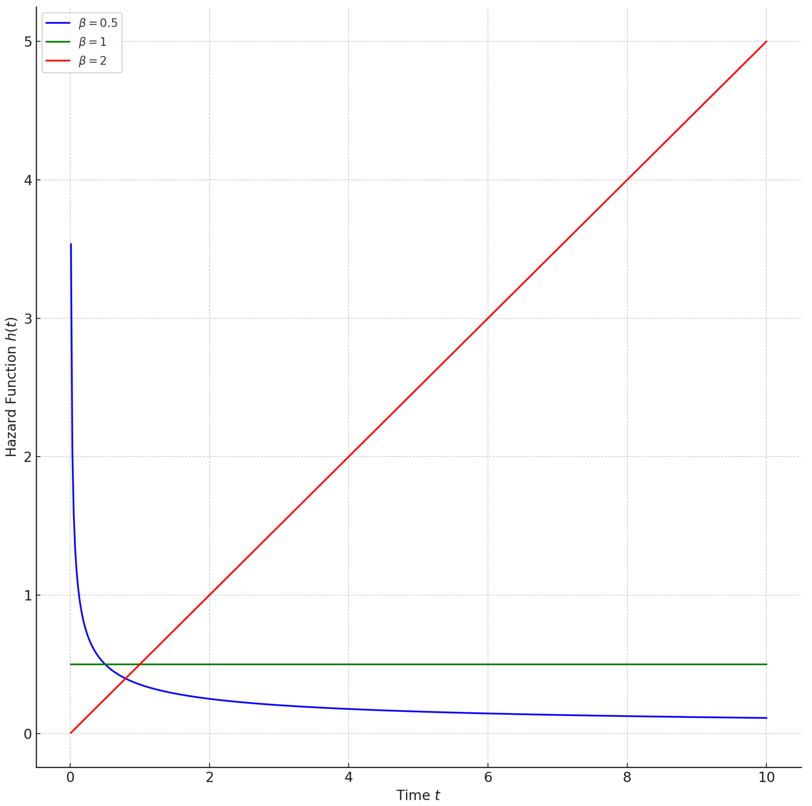
distribution. The hazard rate function
as defined in (4), depends on
. If
the failure rate is constant and given by
, making the NWPD ideal for components with constant failure rates. For
the hazard rate increases with time, modeling components that degrade more quickly. Conversely, for
the hazard rate decreases with time, capturing components that degrade more slowly.
Figure 1 shows the hazard function for different values of
(less than, equal to, and greater than 1), with fixed
and
.
The NWPD is a versatile statistical model that combines the strengths of the Weibull and Pareto distributions to effectively analyze reliability and lifetime data. It offers a flexible framework capable of accommodating diverse hazard rate shapes, including increasing, decreasing, and bathtub-shaped patterns, making it suitable for a wide range of applications. The distribution has gained prominence due to its ability to model real-world phenomena in fields such as engineering, quality control, and survival analysis. Its mathematical properties, such as probability density and cumulative distribution functions, have been extensively studied, along with its reliability measures and stress–strength relationships. Parameter estimation for the NWPD presents unique challenges due to the absence of closed-form solutions, necessitating the use of advanced statistical methods such as maximum likelihood (ML) estimation, Bayesian approaches, and Markov chain Monte Carlo (MCMC) techniques. These features have established the NWPD as a powerful tool in the analysis of complex lifetime data under various censoring schemes including the following: Nasiru and Luguterah [
3] investigated the structural properties of the NWPD, emphasizing its ability to represent varying hazard rate behaviors. Tahir et al. [
4] extended this work by deriving additional mathematical properties, including moments and generating functions, and showcasing the distribution’s utility in reliability and stress–strength applications.
Estimation methods for the NWPD have been a critical area of research. Mahmoud et al. [
5] developed inference procedures for the distribution under progressively Type-II censored data using ML estimation. EL-Sagheer et al. [
6] extended these methods to adaptive Type-II progressive censoring, enhancing the flexibility of the inference framework. Almetwally and Almongy [
7] conducted a comparative study of estimation techniques, demonstrating the efficiency of simulation-based approaches in parameter estimation. They highlighted the robustness of Bayesian estimation methods under different prior assumptions, which has been further explored in recent work by Eliwa et al. [
8]. They introduced Bayesian estimation techniques using Lindley and MCMC methods, incorporating general entropy principles for parameter estimation. Their study addressed challenges related to non-closed-form likelihood functions, providing comprehensive tools for obtaining point estimates and credible intervals (CRIs).
Applications of the NWPD in quality control and reliability have also been widely explored. Al-Omari et al. [
9] proposed acceptance sampling plans based on truncated life tests, demonstrating the distribution’s practicality in industrial quality assurance. Shrahili et al. [
10] developed acceptance sampling plans based on percentiles, applying them to real-world scenarios, such as the breaking stress of carbon fibers. Advanced sampling methodologies have also been investigated. Samuh et al. [
11] introduced estimation methods using ranked set sampling, which enhanced accuracy and efficiency compared to simple random sampling. In the domain of stress–strength reliability analysis, Attia and Karam [
12] derived methods to evaluate
using the NWPD, while Mutair and Karam [
13] extended this to analyze
, showcasing its utility in multi-component reliability systems.
Censoring schemes play a pivotal role in lifetime data analysis and reliability studies, allowing researchers to manage practical constraints while extracting meaningful statistical insights. Among these schemes are the following: in a Type-I censoring scheme, the experiment is terminated at a predetermined time, regardless of how many failures have occurred. This approach is widely used in reliability and survival studies where time constraints or resource limitations dictate the end of the testing period. The exact failure times of all items are not always observed.
Type-II censoring occurs when the experiment continues until a pre-specified number of failures have been observed. Unlike Type-I censoring, the termination is based on the number of failures rather than time. This scheme is advantageous in reliability testing when failure data for a fixed number of components is required to make inferences. Type-II censoring ensures that the data collected provides detailed information about the failure process up to a specific failure count, making it suitable for applications where understanding the failure mechanism is essential.
Progressively Type-II censoring (PT2C) enhances the standard Type-II censoring scheme by allowing for the removal of surviving items at predetermined stages during the experiment. This is performed to reduce the time and cost of the study while still collecting valuable failure data. At each failure point, a subset of the remaining items is randomly withdrawn, and the experiment continues with the remaining items until the desired number of failures is reached. This scheme balances the need for detailed failure data with the practical considerations of testing large sample sizes.
In a progressive first-failure censoring (PFFC) scheme, suppose that
n independent groups, each containing
k items, are subjected to a life-testing experiment starting at time zero. Let
m denote a pre-specified number of failures, and let
represent the censoring scheme (CS) of the groups. At the time of the first observed failure
,
groups, along with the group in which the first failure occurred, are removed from the experiment. After the second observed failure
,
groups, as well as the group experiencing the second failure, are removed from the remaining
groups, and this process continues. The procedure is repeated until the
failure occurs, at which point all remaining groups are removed, where
. The times
, then, represent the independent lifetimes of the PFFC order statistics; see Wu and Kuş [
14]. The observed lifetimes
are defined as the
ith observed failure times among the
m total observed failures from
n groups of size
k items under the specified progressive first-failure censoring scheme
R. If the failure times of the items originally included in the life-testing experiment follow the NWPD with a PDF
and a CDF
, the likelihood function (LF) for the observed data
can be expressed as follows:
The development of advanced statistical models under various censoring schemes has been an active area of research, providing robust methodologies for parameter estimation and reliability analysis. For instance, Kumawat and Nagar [
15] explored the Modi-Exponential distribution under conventional Type-I and Type-II censoring schemes, highlighting its flexibility in modeling lifetime data. Their work presented inference techniques and emphasized the distribution’s applicability to real-world reliability problems, demonstrating its suitability for diverse datasets. Similarly, Almetwally et al. [
16] introduced the Marshall–Olkin Alpha Power Weibull distribution and examined various estimation methods based on Type-I and Type-II censoring. Their findings provided a comparative analysis of classical and Bayesian techniques, underlining the importance of selecting appropriate estimation methods based on the underlying data and application context. Almetwally [
17] further extended the Marshall–Olkin Alpha Power Weibull distribution to its “extended” version, applying it to both Type-I and Type-II censored data. This study offered new insights into parameter estimation techniques, showcasing their effectiveness in capturing the nuances of reliability data. The introduction of flexible distributions like these demonstrates the growing interest in enhancing statistical models to address the limitations of traditional distributions.
Progressive censoring schemes have also garnered significant attention for their practicality and efficiency. Prakash et al. [
18] examined the reduced Type-I heavy-tailed Weibull distribution under a PT2C scheme. Their work addressed the challenges associated with heavy-tailed data and proposed estimation methods that yielded reliable results even under complex censoring scenarios. Similarly, Brito et al. [
19] investigated inference methods for the very Flexible Weibull distribution using PT2C, emphasizing its adaptability in reliability and survival analysis. Muhammed and Almetwally [
20] further contributed to this area by developing Bayesian and non-Bayesian estimation methods for the shape parameters of new versions of the bivariate inverse Weibull distribution under PT2C. Their findings highlighted the robustness of Bayesian methods in capturing the uncertainties associated with censored lifetime data.
The PFFC scheme has become an essential tool in statistical modeling, especially for reliability analysis and lifetime data estimation. The literature on this topic provides a wide array of methodologies and applications, particularly focusing on parameter estimation, stress–strength reliability, and distribution-specific analyses under this scheme. Also, Saini et al. [
21] explored stress–strength reliability for the generalized Maxwell failure distribution under PFFC. Their study emphasized the practical application of this censoring scheme in reliability engineering, particularly in systems where the failure process follows complex distributions like the generalized Maxwell. They developed estimation techniques that allowed for the reliable inference of stress–strength reliability parameters, which is critical in evaluating the safety and performance of engineering systems.
In a similar vein, Saini and Garg [
22] examined both non-Bayesian and Bayesian estimation techniques for stress–strength reliability based on the Topp-Leone distribution under PFFC. Their work compared the effectiveness of different estimation approaches, showcasing how Bayesian methods can improve the accuracy of parameter estimation when prior information is available. Dube et al. [
23] studied the generalized inverted exponential distribution under PFFC, emphasizing its relevance in modeling real-world systems where failures occur intermittently and unpredictably. Their findings contributed to the broader understanding of how flexible distributions can be utilized to model failure data accurately under the PFFC.
The study of multi-component systems under PFFC was advanced by Kohansal et al. [
24] who focused on stress–strength reliability for such systems. Their research showed how the scheme could be effectively applied to complex systems with interdependent components, where the reliability of the system depends on the strengths and failures of its individual parts. This work has significant implications for industries where system reliability is critical, such as aerospace and automotive engineering. Finally, Ramadan et al. [
25] introduced a methodology for estimating the lifetime parameters of the Odd-Generalized-Exponential–Inverse-Weibull distribution using PFFC. Their study not only addressed the challenges of parameter estimation for this complex distribution but also demonstrated its practical application through a real-world dataset, reinforcing the importance of flexible and adaptable models in lifetime analysis.
In practical reliability applications, many systems exhibit non-monotonic failure patterns, most notably the widely observed bathtub-shaped hazard function, which captures the early-life failure, useful-life, and wear-out phases of components. Modeling such behaviors is essential for accurate reliability assessment and maintenance planning. The NWPD is well-suited for this purpose, as its flexible parameterization allows it to accommodate increasing, decreasing, and bathtub-shaped hazard rate structures, thereby enhancing its applicability in diverse reliability scenarios. Furthermore, real-world systems often consist of interacting or dependent components, where failures in one component may influence the reliability of others. Addressing such dependencies is crucial in multistate system modeling and in the estimation of system reliability and maintenance costs. In this regard, we incorporate the foundational works of Blokus [
26], who provided a detailed treatment of multistate system reliability with dependencies, and Romaniuk and Hryniewicz [
27], who examined maintenance cost estimation under imprecise environments for systems with U-shaped (bathtub) hazard functions. These studies complement our current research by emphasizing the need for adaptable statistical models that can handle complex failure behaviors and interdependencies. Our work contributes to this growing body of literature by demonstrating the effectiveness of the NWPD under progressive first-failure censoring, a practical scheme for reducing cost and time in life-testing experiments.
Progressive censoring schemes, particularly PFFC, have gained significant attention for their practicality in life-testing experiments. These schemes provide an efficient way to manage time and cost constraints while still yielding meaningful insights into failure mechanisms. However, statistical inference under such schemes presents unique challenges due to the complex nature of the likelihood functions, which often lack explicit closed-form solutions. While it is true that accelerated life testing is important for many modern reliability applications, PFFC remains relevant in scenarios where test cost, sample size, or ethical constraints limit the possibility of extensive failure testing. As shown in the literature (e.g., Wu and Kuş [
14], Saini et al. [
21], Ramadan et al. [
25]), the PFFC scheme provides practical benefits, particularly in quality control and multi-component reliability systems, by allowing for the early removal of groups to reduce time and cost. Moreover, PFFC data structures facilitate the development of robust inferential procedures. Our study leverages the flexibility of the new Weibull–Pareto distribution under this censoring framework to fill a gap in the literature where such combinations have not been fully explored. Moreover, the PFFC scheme is particularly meaningful in the reliability context, in which early failures are the major evidences for the quality of the product. Although life testing with acceleration is common, many applications (e.g., pharmaceuticals, avionics) only have access to first failure data for ethical or economic reasons. PFFC is capable of reducing the time and cost of experiments, and even statistical information is enough especially for high-reliability products. The PFFC scheme is recommended for the case where the component’s cost is extremely lower than the testing-time cost.
This paper focuses on estimating the lifetime parameters of the NWPD and some reliability characteristics under PFFC. ML estimation methods are developed to estimate the model parameters and survival and hazard rate functions. To address the computational challenges associated with these methods, iterative numerical algorithms such as Newton–Raphson (N-R) are employed. Furthermore, Bayesian estimation techniques, incorporating various loss functions and independent gamma priors, are explored to provide robust point estimates and CRIs. The theoretical contributions of this work are complemented by an application to a real-world dataset, illustrating the practical value of the proposed methods. The findings provide a comprehensive framework for statisticians and reliability engineers seeking to model and analyze lifetime data with the new Weibull–Pareto distribution under censoring schemes.
This paper is structured as follows:
Section 2 focuses on the ML estimates (MLEs) for the parameters of the NWPD and their approximate confidence intervals (ACIs).
Section 3 employs the MCMC method to derive Bayesian estimates (BEs) for these parameters, as well as for the survival and hazard rate functions, using independent gamma priors. Additionally, it provides the highest posterior density credible intervals (HPDCRIs) based on the MCMC results.
Section 4 presents a Monte Carlo simulation to assess the proposed estimators in terms of mean squared error (MSE), average interval width (AIW), and coverage probability (CP).
Section 5 illustrates the application of the methodology using real-world datasets. Lastly,
Section 6 concludes with a summary of the findings.
2. Maximum Likelihood Estimation
Maximum likelihood estimation is a fundamental method in statistical inference used to estimate unknown parameters of a probability distribution by maximizing the likelihood function based on observed data. One of the key properties of MLE is consistency, meaning the estimator converges to the true parameter value as the sample size increases. It is also asymptotically efficient, achieving the lowest possible variance among all unbiased estimators under regularity conditions, and asymptotically normal, which simplifies inference in large samples. MLE is particularly valued for its flexibility and broad applicability, making it a preferred tool for statisticians in fields such as biostatistics, econometrics, and machine learning. Compared to other methods like the method of moments, which is simpler but often less efficient, or Bayesian estimation, which incorporates prior knowledge but may be computationally intensive, MLE offers a strong balance between theoretical rigor and practical performance. Due to these advantages, MLE continues to be one of the most extensively studied and applied estimation techniques in modern statistics. This section is dedicated to applying MLE to derive both point and interval estimates for the unknown parameters
and
, along with
and
based on the PFFC dataset modeled by the NWPD. Let
be a PFFC order statistics of size
m from the NWPD with a pre-fixed CS
. From Equations (1), (2) and (5), the LF, denoted by
, is given by
The log-LF, denoted by
, without the additive constant, can be written as
By setting the first partial derivatives of Equation (
7) with respect to
and
equal to zero, we derive
and
From Equation (
8), the MLE
of
can be expressed as a function of the MLEs
and
of
and
, given by
Obtaining the MLEs for
and
is challenging because the nonlinear Equations (9)–(11) do not have closed-form analytical solutions. Consequently, we suggest using a numerical approach, such as the Newton–Raphson iteration algorithm, to estimate the unknown parameters
and
. The proposed algorithm is outlined as follows:
- 1.
Begin with initial parameter values for and set the iteration index .
- 2.
In the
iteration, evaluate the gradient vector
at
,
along with the observed Fisher information matrix
corresponding to the parameters
and
.
where
and
- 3.
Assign
where
symbolizes the matrix’s inverse
given in Equation (
12).
- 4.
Increment the iteration counter by setting and repeat the procedure starting from Step 1.
- 5.
Repeat the iterative process until the difference falls below a specified convergence threshold. The resulting values of and at convergence are taken as the MLE of the parameters, denoted by , , and .
Moreover, for a specified value of
t, the MLEs of
and
, as defined in Equations (3) and (4), can be obtained by utilizing the invariance property of MLEs, substituting the estimates
,
, and
in place of
and
, respectively, as follows:
and
The NR method is employed to obtain the MLEs due to its rapid convergence properties and effectiveness in handling smooth, differentiable likelihood functions. The NR algorithm leverages both the first and second derivatives (i.e., the score function and observed Fisher information matrix), allowing for efficient iterative updates that converge quadratically near the optimum. This is particularly advantageous in our context, where the log-likelihood function derived from the NWPD under progressive first-failure censoring is nonlinear but has well-defined gradients. While alternative numerical methods such as gradient descent or quasi-Newton schemes (e.g., BFGS) could be applied, they often converge more slowly or require additional tuning. Given that the required derivatives can be computed in closed form, NR provides an accurate and computationally efficient solution for parameter estimation in this setting.
To ensure the reliable convergence of the Newton–Raphson algorithm, initial values for the parameters ( ) were carefully selected based on practical estimation techniques. Specifically, initial guesses were obtained using two approaches: (i) method-of-moments estimators calculated from complete or uncensored data when available, and (ii) a coarse grid search over the parameter space to identify values that yielded a high log-likelihood. These starting points were found to provide stable convergence across different sample sizes and censoring schemes. Sensitivity analyses further confirmed that, under moderate sample sizes, the NR algorithm was generally robust to variations in initial values. However, in cases of small or highly censored samples, convergence speed and accuracy were more sensitive, which underscores the importance of informed initialization. In numerical computation, the NR algorithm could fail to obtain proper estimators when the parameters cannot be solved independently. The log-likelihood equation is complicated due to using a three-parameter model and the PFFC censoring scheme. Carefully checking the estimation results with different initial solutions is suggested.
2.1. Existence and Uniqueness of the MLEs
In statistical inference, the existence and uniqueness of the MLEs are regarded as essential properties. In this subsection, we establish the necessary and sufficient conditions for the existence of the MLEs for arbitrary PFFC data under the NWPD model. To do so, we examine the behavior of Equations (8)–(10) over the positive real interval .
For Equation (
8), when
, we have
, but when
, we have
, for
;
,
,
Similarly, for Equation (
9), when
, we have
, but when
, we have
, for
Similarly, for Equation (
10), when
, we have
, but when
, we have
for
,
,
Thus, on for , there exists at least one positive root for 0. Furthermore, we find that the second partial derivatives of ℓ w.r.t. and given in Equations (13), (16) and (18) are always negative; Equations (8)–(10) have a unique solution, and this solution represents the MLEs of and . Hence, we conclude that is a continuous function on , and it monotonically decreases from ∞ to negative values. This demonstrates the existence and uniqueness of the MLEs of and .
2.2. Approximate Confidence Intervals
Approximate confidence intervals are a fundamental tool in statistical inference used to estimate the range within which an unknown parameter is likely to lie based on sample data. These intervals are typically derived using the asymptotic distribution of an estimator, such as the normal distribution in the case of MLEs. Among their key properties are asymptotic validity, computational simplicity, and broad applicability to complex models and large datasets. The main advantage of ACIs lies in their ease of construction, especially when exact methods are analytically intractable. Statisticians have shown strong and consistent interest in this approach due to its flexibility and efficiency, particularly in high-dimensional or real-world applications where exact methods are either unavailable or too restrictive. Compared to exact confidence intervals, which offer precise coverage in small samples but are often limited to simple distributions, approximate intervals provide a practical alternative with good performance in large samples. In contrast to Bayesian CRIs, which depend on prior information and have a different interpretive framework, ACIs are rooted in the frequentist paradigm and do not require prior assumptions. Therefore, despite some limitations in small samples, ACIs remain widely used and highly regarded in both theoretical and applied statistics. In this subsection, we derive the ACIs for the vector of the unknown parameters
of the NWPD under the asymptotic normal distribution of the MLEs (see Vander Wiel and Meeker [
28]) and using the asymptotic variance-covariance matrix (AVCM). The AVCM of the MLEs
of
is obtained by taking the inverse of the observed FIM given in Equation (
12) as follows:
where
;
i,
, are defined in Equations (13)–(18). The ACIs for
are based on the multivariate normal distribution with mean
and AVCM
. Accordingly, the
ACIs for
can be constructed as follows:
where
is the percentile of the standard normal distribution
with right-tail
.
2.3. Delta Technique
The Delta technique (DT) is a widely used technique for deriving ACIs for functions of estimators, particularly when those functions are nonlinear. By utilizing a first-order Taylor series expansion around the point estimates of the parameters, the DT transforms a nonlinear function into a linear approximation, facilitating variance estimation. The resulting variance of the transformed function is then approximated using the gradient (Jacobian) of the function evaluated at the estimated parameters, in conjunction with the estimated variance–covariance matrix of the parameters. This method relies on the asymptotic normality of the estimators and provides a practical solution for inference in complex models; refer to Greene [
29] for details. Now, we employ the DT to approximate the variances of
and
as follows: Let
and
be two quantities expressed in the following forms:
where, based on the formulations given in Equations (3) and (4),
and
Apply the provided formulas to estimate the approximate variances of
and
:
where
and
are the transpose matrices of
and
given in Equation (
24), and
is derived from Equation (
22) for
. Finally, the
ACIs for
and
can be derived using the following expressions:
The lower bounds of the ACIs for the vector of the parameters
given in Equation (
23) may be negative, which conflicts with the requirement that
0. In such cases, substituting a negative value with zero may be considered. To deal with this defect in the accuracy of the normal approximation, Meeker and Escobar [
30] introduced a solution by using a log-transformed MLE based on ACIs combined with the DT. Specifically, the log-transformed MLEs satisfy
, where
. Thus, the
log-transformed ACIs (LACIs) for the vector of the parameters
are computed as follows:
where
is defined in Equation (
22). Similarly, the
LACIs for
can be expressed as
3. Bayesian Estimation
Bayesian estimation (BE) is a statistical technique that incorporates prior knowledge with observed data to produce parameter estimates based on the posterior distribution. A key property of BE is its dependence on the chosen loss function, which allows it to adapt to different decision-making contexts. Under symmetric loss functions (SLFs), such as the squared error (SE) loss, the Bayes estimator typically corresponds to the posterior mean, offering balanced and efficient estimates. In the case of asymmetric loss functions (ALFs) where the costs of overestimation and underestimation differ, the Bayes estimator adjusts accordingly, often yielding the posterior median or mode, depending on the specific form of the loss. This flexibility is a major advantage over classical estimation methods like MLE, which do not account for the consequences of estimation errors. Additionally, BE provides a full probabilistic description of uncertainty, offering richer inference through posterior distributions and credible intervals (CRIs). The increasing availability of computational tools, such as Markov chain Monte Carlo (MCMC), has made Bayesian methods more accessible and practical, leading to growing interest among statisticians. Compared to traditional frequentist methods, BE is often more informative, especially in small-sample situations or when prior knowledge is relevant, making it a valuable alternative for both theoretical research and applied statistics.
In BE, the initial stage involves examining the influence of the prior distribution on the resulting inference. In this context, we adopt the gamma distribution as the prior due to its suitability for modeling positive, continuous parameters, particularly those related to rates or precision in exponential family distributions. The gamma prior is defined by two parameters: the shape and the scale (or alternatively, rate), which together determine its flexibility and the concentration of prior belief. One of the main advantages of using the gamma distribution is its conjugacy with several common likelihood functions, such as the exponential and Poisson, which ensures that the posterior distribution remains within the same family. This conjugacy leads to simplified analytical derivations and efficient computation, especially when updating beliefs with observed data. Moreover, the gamma distribution’s ability to represent a wide range of prior beliefs from the vague to the highly informative makes it an effective and versatile choice in Bayesian analysis. Its mathematical tractability and adaptability have contributed to its popularity among statisticians when performing Bayesian inference involving non-negative parameters. In this section, we obtain the BEs and construct CRIs for the parameters
as well as
and
, considering both symmetric and asymmetric loss functions under the PFFC samples from the NWPD. Let us assume that the parameters
and
are mutually independent random variables and follow the gamma prior distributions with PDFs as follows:
where the hyperparameters
for
are specified and represent prior beliefs about
. Consequently, the joint prior density function of
is expressed as
Using Bayes’ theorem and Equations (6) and (30), the joint posterior density function of the parameters is
The BEs for any function of the parameters
and
, denoted by
, can be derived under various loss functions depending on the decision-making context. Specifically, under the squared error (SE), the linear exponential (LINEX) and the general entropy (GE) loss functions, are given, respectively, by the following formulae:
and
For detailed derivations and a theoretical background, see Varian [
31], Calabria and Pulcini [
32], and Gelman, et al. [
33]. In Bayesian estimation under asymmetric loss functions like LINEX and GE, the parameter
controls the degree and direction of asymmetry. Choosing
appropriately is crucial, as it reflects the cost structure associated with underestimation vs. overestimation. Here is how
is generally determined:
- 1.
Decision theoretic interpretation:
- (a)
penalizes underestimation more than overestimation.
- (b)
penalizes overestimation more than underestimation.
- (c)
reduces LINEX or GE loss to symmetric squared error loss.
- 2.
Thus, should be chosen based on the practical consequences of the estimation error:
- (a)
If underestimating a failure rate could lead to critical system breakdowns (e.g., in safety systems), choose .
- (b)
If overestimating would lead to overly conservative or costly decisions, choose .
In our current version, we considered
as representative values, as commonly practiced in the Bayesian literature (e.g., Varian [
31], Calabria and Pulcini [
32]). As the Bayes estimators under SE, LINEX, and GE loss functions do not have closed-form solutions, numerical methods are required to obtain them. To address this, we propose employing the MCMC approach, which is well-suited for sampling from complex posterior distributions. By generating a large number of samples from the joint posterior distribution of
and
, the BEs for these parameters can be approximated efficiently under the chosen loss functions. This approach provides a flexible and practical framework for Bayesian computation when analytical solutions are intractable.
MCMC Approach
Markov chain Monte Carlo is a class of powerful simulation-based algorithms used in BE to approximate complex posterior distributions when analytical solutions are intractable. MCMC methods work by constructing a Markov chain whose stationary distribution is the target posterior distribution, allowing for the generation of dependent samples that, over time, represent the true posterior. These samples can then be used to estimate Bayes estimators, credible intervals, and other quantities of interest. There are several types of MCMC algorithms commonly used in Bayesian analysis. The Metropolis–Hastings (MH) algorithm is a general-purpose method that proposes new samples and accepts or rejects them based on an acceptance probability, ensuring convergence to the desired distribution. The Gibbs sampler (GS), a special case of MH, is particularly effective when the full conditional distributions of parameters are known and easy to sample from. To begin with, the full conditional posterior distributions for the parameters
and
can be represented as follows:
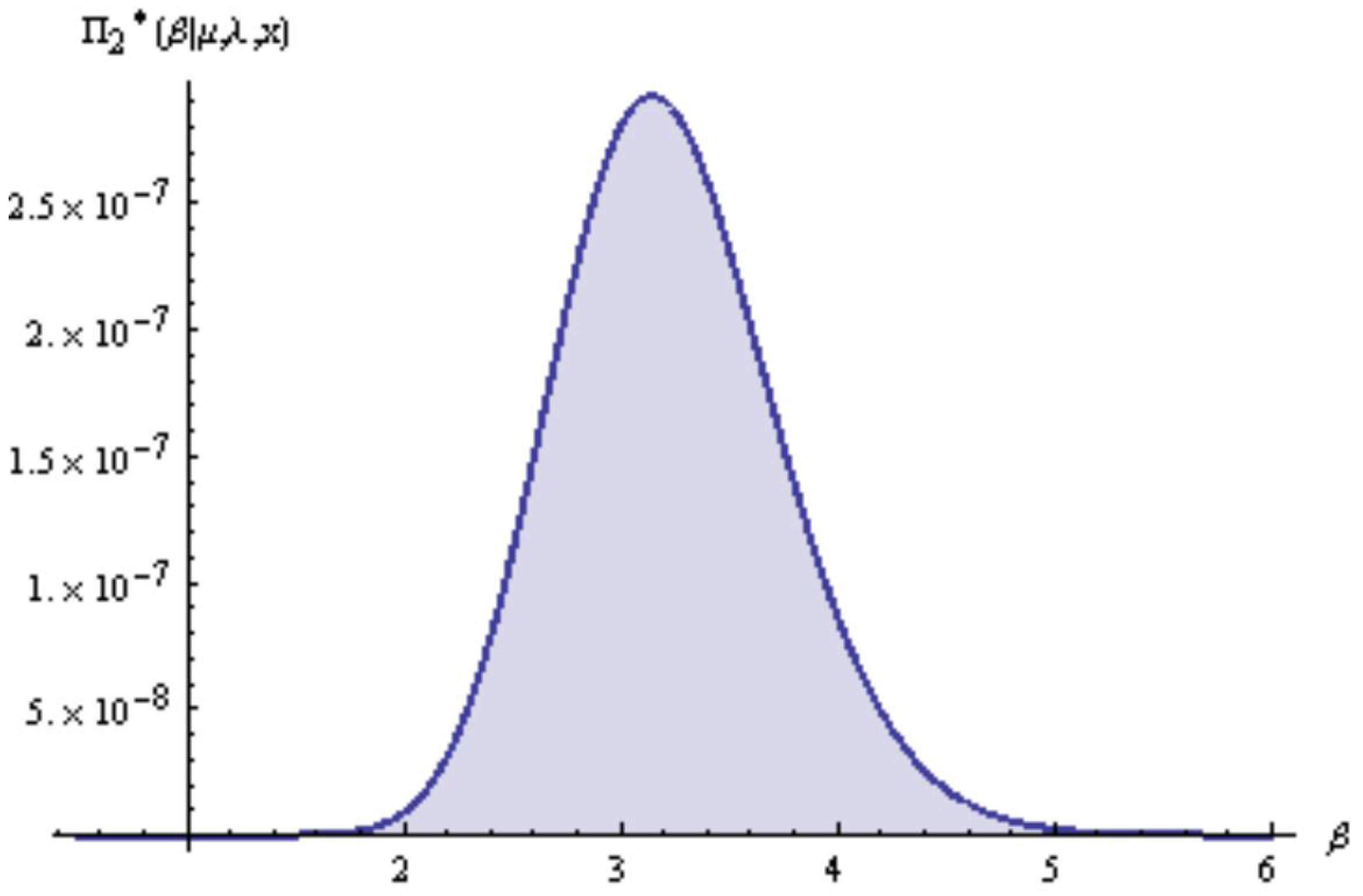
and
It is evident that, as shown in Equation (
35), the full conditional posterior distribution of the parameter
follows a gamma distribution with shape parameter
and scale parameter
. Hence, generating samples from
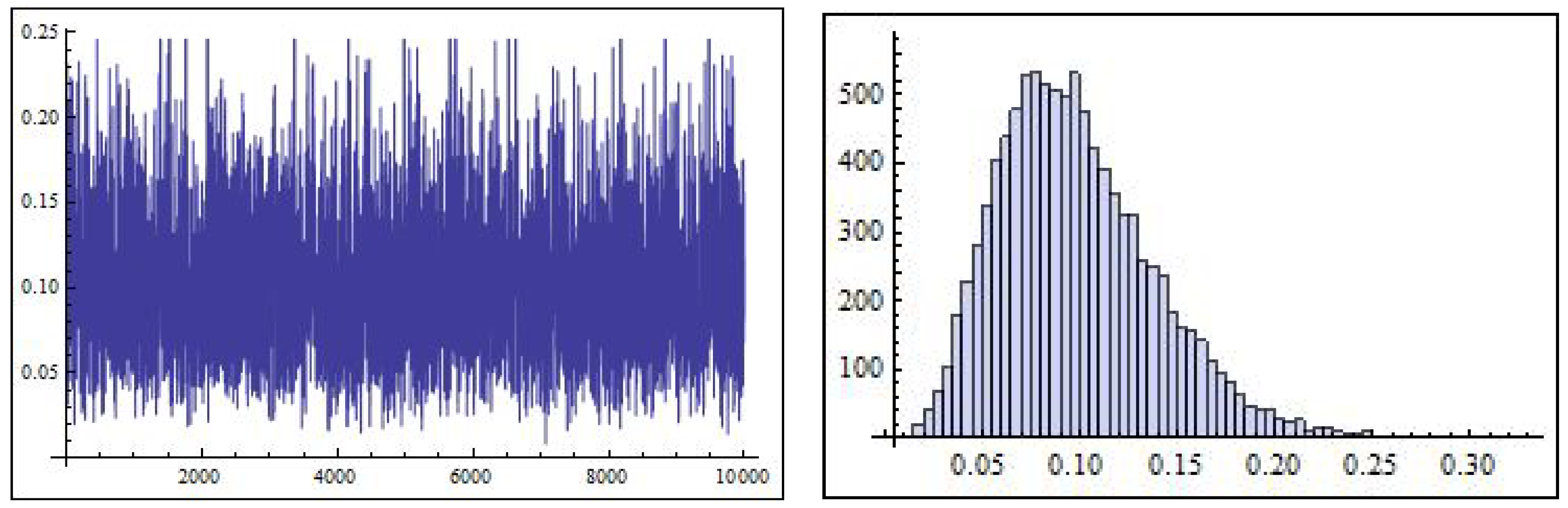
can be efficiently accomplished using any standard gamma sampling routine. On the other hand, Equations (36) and (37) do not correspond to any well-known distributions; however, their empirical density plots indicate approximate normality, as illustrated in
Figure 2 and
Figure 3. Consequently, the MH algorithm is an appropriate choice for drawing samples from
and
. Following the approach outlined by Metropolis et al. [
34] and Hastings [
35], the sampling procedure combines the GS strategy with the MH algorithm as discussed in Tierney [
36]. This hybrid method utilizes a normal proposal distribution to facilitate sample generation from the posterior and proceeds according to the following iterative steps:
- Step 1.
Begin by assigning initial values to the parameters, say , and set the iteration index .
- Step 2.
Generate from the gamma distribution .
- Step 3.
Apply the following MH algorithm to generate from and from , with normal proposal distributions and , respectively. Proceed as follows:
- i.
Draw a proposal from and from .
- ii.
Evaluate the acceptance probabilities:
- iii.
Generate two random numbers and from the Uniform distribution.
- iv.
If , accept the proposal and put ; otherwise, put .
- v.
If , accept the proposal and put ; otherwise, put .
- Step 4.
For a given
t, employ
and
to calculate the survival
and hazard rate
functions as
and
- Step 5.
Set .
- Step 6.
Implement the steps from 3 to for a total of M iterations. To ensure the convergence and eliminate the affection of the selection of initial values, the first simulated variants are removed. The required number of samples are , , for sufficiently large values of M from an approximate posterior sample that can be utilized to develop the BEs using the remaining samples.
- Step 7.
Based on the SE, LINEX, and GE loss functions, the approximate BEs of the parameter vector
can be expressed as
and
where
is a burn-in sample.
- Step 8.
To construct the HPDCRIs for the parameter
, sort
in ascending order as
. Accordingly, the
Bayesian symmetric HPDCRIs for
can be given by (see Chen and Shao [
37]).
Note: In the implementation of the MCMC algorithm, the initial values for the parameters were set to their corresponding MLEs. This initialization strategy is commonly adopted in Bayesian computation because MLEs often lie near the mode of the posterior distribution, especially under moderately informative priors. Starting the Markov chains from these values helps accelerate convergence, reduce the required burn-in period, and improve sampling efficiency. This approach is particularly useful when the posterior is unimodal and relatively symmetric, as is the case in our model under the chosen prior settings.
4. Simulation Study and Comparison
A simulation study plays a pivotal role in evaluating and comparing estimation techniques by offering a flexible and reproducible environment to assess their behavior under various controlled settings. Through the generation of synthetic data that mimic real-life scenarios, researchers can observe how estimation methods perform in terms of bias, precision, and interval accuracy when confronted with known parameters and varying sample characteristics. This structured approach not only reveals the strengths and limitations of each method but also guides the refinement of estimation procedures for broader applicability and greater reliability. In this section, we evaluate the proposed BEs in comparison with the MLEs using a comprehensive Monte Carlo simulation framework. The study explores multiple combinations of sample sizes
n, group counts
m, and censoring schemes
R, employing the algorithm by Balakrishnan and Sandhu [
38] with CDF
where
k is the same number of units within each group, to generate PFFC samples from the NWPD with fixed parameters
. The theoretical values
and
are computed at
, yielding
and
, respectively. Note: The value
was selected for evaluating the survival and hazard functions because it lies near the lower quantile of the NWPD with the chosen parameter set
. This placement allows for assessing the estimators’ performance in the early failure region, which is particularly relevant in reliability analysis where early-life behavior is often critical. Selecting
t in this range ensures that the resulting estimates of
and
are both nontrivial and informative under the PFFC framework. The estimators’ accuracy is assessed via the mean square error (MSE), defined by
for
, and
or
. Further evaluation includes the average widths (AWs) and coverage probabilities (CPs) of asymptotic confidence intervals (ACIs) and Bayesian credible intervals (CRIs), where the latter are obtained from
12,000 MCMC samples after discarding the first
2000 as burn-in. Informative gamma priors are specified with hyperparameters
for
. Simulations are conducted for two group sizes
and three censoring schemes: CS1, where all censoring is assigned to the first group
for
; CS2, where censoring is split between the middle two groups or centered on the middle group depending on the parity of
m, i.e., (
for
and
if
m is even;
for
if
m is odd); and CS3, where censoring is applied to the last group
,
for
. For instance, for
, the configurations are CS
, CS
, and CS
; for
, they become CS
, CS
, and CS
. The simulation results, summarized in
Table 1,
Table 2,
Table 3,
Table 4,
Table 5,
Table 6,
Table 7 and
Table 8, provide valuable insights into the behavior and effectiveness of the estimators under various settings. The results give rise to several noteworthy observations:
- 1.
- 2.
Analysis of all tables reveals that increasing the group size k leads to higher MSEs and AWs for the parameter vector .
- 3.
Among the estimation techniques evaluated, BEs demonstrate the lowest MSEs and AWs for the parameter vector , signifying their superior accuracy over MLEs.
- 4.
The BE under the GE loss function with achieves the most precise estimates for , as reflected by its reduced MSEs.
- 5.
Using the LINEX and GE loss functions with results in improved BEs compared to , evidenced by consistently lower MSEs.
- 6.
Under the SE loss function, BEs for the parameter vector outperform those obtained using the LINEX and GE loss functions with due to their smaller associated MSEs.
- 7.
Given fixed sample sizes and observed failures, the CSI scheme proves to be the most effective, offering the smallest MSEs and AWs.
- 8.
MLE and Bayesian methods provide very similar estimates, with both having ACIs with high CPs of around . However, Bayesian CRIs achieve the highest CPs.
Although Bayesian CRIs are generally expected to offer improved interval estimation particularly when informative priors are used, the simulation and real-data results in this study revealed only marginal gains over frequentist ACIs. This can be attributed to several factors. First, the gamma priors adopted for the model parameters, while informative, were only moderately concentrated and, thus, did not exert a strong influence relative to the likelihood, especially as sample size increased. Second, the PFFC scheme inherently reduces the amount of observed information, limiting the precision achievable by any method. Third, ACIs constructed via the asymptotic normality of MLEs tend to perform well under large or moderately sized samples, as in our study. As a result, the CRIs and ACIs exhibited comparable widths and coverage probabilities. This convergence highlights that, under moderate prior informativeness and sufficient data, Bayesian and frequentist approaches may yield similar inference in terms of interval estimation.
5. Application to Real-Life Data
The practical validation of theoretical models through real-world data is crucial to assess their applicability and robustness. While theoretical frameworks lay the groundwork for statistical analysis, empirical data enables researchers to evaluate their performance under actual conditions. In this section, we demonstrate the practical utility of the proposed inferential procedures by applying them to a real dataset comprising 88 failure time observations of automobile windshields. This dataset, originally compiled by Blischke and Murthy [
39] and later referenced by Murthy et al. [
40], serves as an effective benchmark for model assessments. To measure the adequacy of the fitted distributions, the Kolmogorov–Smirnov test was employed, yielding a distance of
and a high
p-value of
when applied to the NWPD model with the estimated parameters
. This result suggests a superior fit compared to alternative models. Now, we implement a detailed comparison with other common lifetime models, namely the Weibull, log-logistic, and exponential distributions. Goodness-of-fit metrics such as the Akaike Information Criterion (AIC), Bayesian Information Criterion (BIC), and log-likelihood values are provided in a new table (
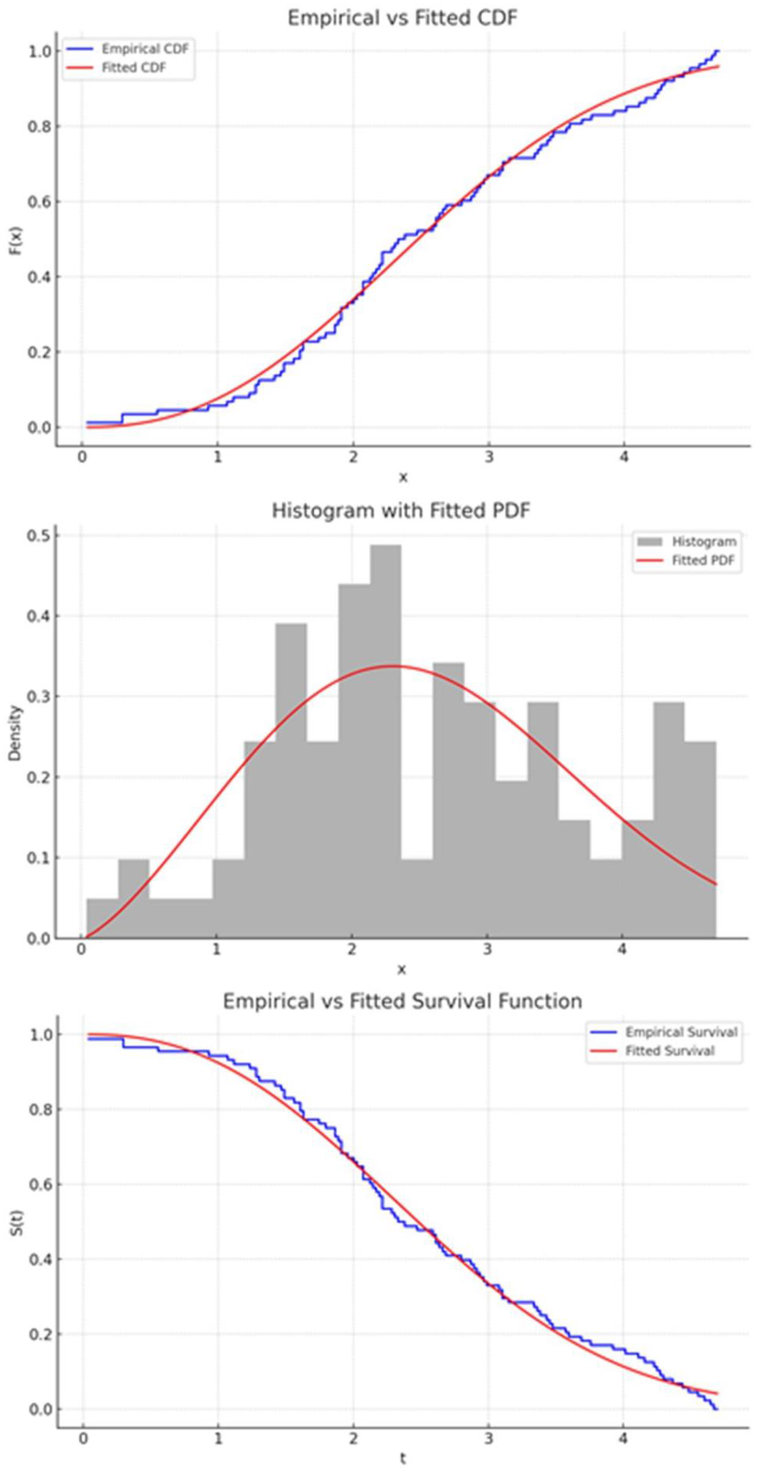
Table 9). These results support the claim that the NWPD offers superior flexibility and fit for the real dataset under analysis.
The goodness-of-fit results in
Table 9 demonstrate that the NWPD model achieves the lowest values for AIC (
) and BIC (
), along with the highest log-likelihood (
) among all compared models. These metrics collectively indicate a better balance between model fit and complexity, supporting the conclusion that the NWPD provides a superior representation of the observed data compared to the Weibull, log-logistic, and exponential alternatives. This highlights the flexibility of the NWPD in capturing the underlying failure behavior in the presence of censoring. Supporting plots, including the empirical vs. fitted CDF, histogram with fitted PDF and empirical vs. fitted survival function shown in
Figure 4 visually reinforce the NWPD model’s suitability. For additional analysis, the dataset was randomly divided into 22 groups, each containing 4 failure time observations, organized as follows: {(0.040, 1.281, 1.505, 1.506), (0.301, 1.303, 1.432, 1.480), (1.568, 1.615, 1.619, 1.652), (2.135, 4.278, 4.305, 4.376), (0.309, 4.121, 4.167, 4.255), (1.652, 3.779, 3.924, 4.035), (0.557, 1.757, 1.866, 1.899), (0.943, 2.038, 2.085, 2.085), (1.795, 1.911, 1.912, 1.914), (1.070, 3.578, 3.595, 3.699), (1.876, 1.981, 2.097, 2.190), (1.124, 2.194, 2.223, 2.224), (1.248, 3.166, 3.344, 3.376), (2.010, 4.449, 4.485, 4.570), (2.135, 3.103, 3.114, 3.117), (2.154, 4.602, 4.663, 4.694), (2.688, 2.823, 2.890, 2.902), (2.385, 2.962, 2.964, 3.000), (2.625, 2.632, 2.646, 2.661), (2.610, 2.229, 2.300, 2.324), (2.349, 2.481, 2.934, 3.385), (4.240, 3.443, 3.467, 3.478)}. A PFFC sample, denoted by
is constructed by dividing the original dataset into
groups, each containing
units. These groups yield outcomes recorded as
(2, 2, 2, 2, 0, 1, 1, 1, 1, 0), resulting in
recorded first-failure times, while the remaining
groups are excluded. This yields the PFFC sample
{0.040, 1.652, 1.795, 1.876, 2.010, 2.135, 2.135, 2.385, 2.61, 4.240}. Using this sample, MLEs and
ACIs for the parameters
and
are presented in
Table 10 and
Table 11. For Bayesian estimation, non-informative gamma priors are assumed for
and
, with hyperparameters
and
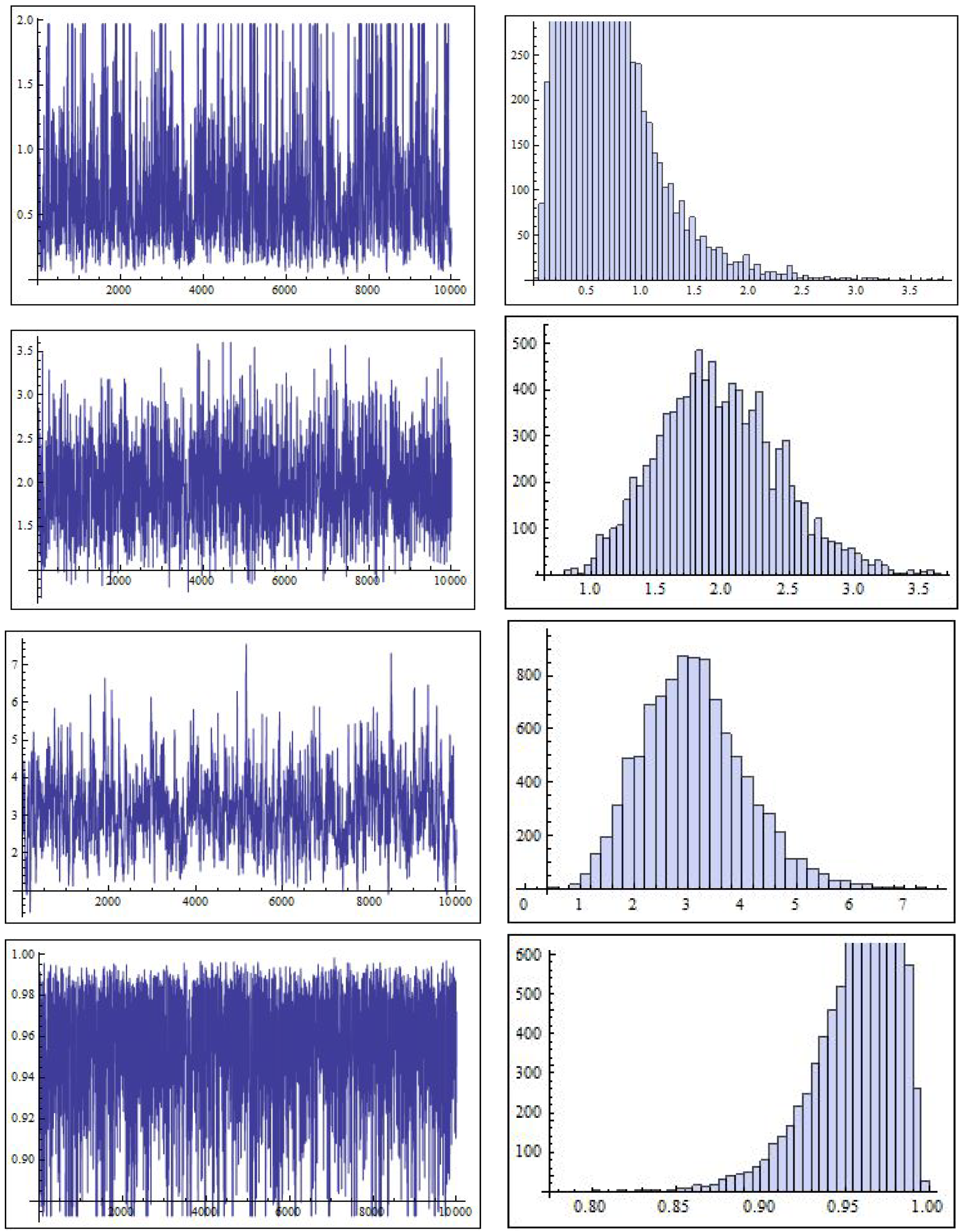
, reflecting the absence of prior knowledge. The posterior distributions are explored via MCMC, employing the MH algorithm integrated with Gibbs Sampling. Initial values for the parameters were set using the MLEs, and a total of 12,000 MCMC iterations were run, with the first 2000 discarded as burn-in to reduce dependence on initial values. The Bayesian estimates and their corresponding
CRIs, in addition to some statistical properties, are summarized in
Table 10,
Table 11 and
Table 12. We can observe the convergence in the MCMC technique through the trace plots and the histograms of the parameters, which are shown in
Figure 5. The value
was chosen because it falls near the lower quantile of the observed failure times in the real dataset. Using this value allows the
and
estimates to be interpreted at a representative central point in the failure time distribution. Overall, the model shows excellent fit to the data, as confirmed by visual assessments. The MLE and Bayesian estimates align closely, with all point estimates residing within their respective intervals, and only minor differences in interval widths indicating consistent and reliable inference.
6. Conclusions
This paper presents a comprehensive framework for estimating the parameters of the NWPD under the PFFC scheme, a censoring mechanism that offers practical flexibility in reliability testing. MLEs for the distribution’s parameters and survival and hazard rate functions are derived and numerically obtained using the Newton–Raphson algorithm due to the lack of closed-form solutions. ACIs are constructed using asymptotic properties of the MLEs, supported by the Fisher information matrix and the Delta method. BE procedures are also explored under symmetric and asymmetric loss functions, incorporating independent gamma priors. MCMC techniques, including the MH algorithm, are employed to obtain Bayes estimates and the highest posterior density credible intervals. A Monte Carlo simulation study was conducted to compare the performance of the proposed estimators. The results demonstrated that Bayesian methods, particularly under the GE loss function with positive skew, outperformed MLEs in terms of MSE and interval precision, especially for small to moderate sample sizes. Finally, the practical applicability of the proposed methods was validated using a real dataset, confirming the suitability and robustness of the NWPD under PFFC. The developed inference techniques offer valuable tools for practitioners and researchers in reliability analysis, especially when dealing with complex lifetime data and censoring constraints.
In practice, the choice between MLE and Bayesian estimation, as well as the selection of an appropriate loss function, should be guided by the structure of the data, the availability of prior knowledge, and the decision-making context. MLE is advantageous for its computational simplicity and strong asymptotic properties, particularly when large sample sizes are available and prior information is limited or unavailable. Conversely, Bayesian methods offer greater flexibility by incorporating prior beliefs and allowing for tailored loss functions. For instance, the squared error loss function is suitable when over- and under-estimation carry equal risk, while the LINEX and GE loss functions are more appropriate in asymmetric risk settings. Our simulation results suggest that the GE loss function with often yields the most accurate Bayesian estimates under PFFC. Thus, practitioners are encouraged to align their estimation strategy with the specific goals of the analysis, the nature of the loss associated with estimation errors, and the level of prior information available.
Based on the simulation findings, we discover that a sample size of at least 30 with a censoring scheme that affects 30–40% of observations results in stable estimation. We propose the following rule: add at least 10 uncensored observations for each additional parameter above three. For guidance, refer to
Table 13.
This study has several limitations that should be acknowledged. First, the construction of ACIs relies on asymptotic properties, which may not perform optimally in small samples. Second, the empirical validation is based on a single real dataset, which may limit the generalizability of the results. Third, the simulation study explores only a limited set of parameter configurations. To address these limitations, future research could involve applying the proposed methods to diverse datasets, investigating the impact of alternative prior distributions in Bayesian analysis, and developing more efficient computational techniques for parameter estimation under PFFC schemes.


