Composite Continuous High-Order Nonsingular Terminal Sliding Mode Control for Flying Wing UAVs with Disturbances and Actuator Faults

Abstract

Flying wing UAVs are widely used in both civil and military areas and they are vulnerable to being affected by multi-source disturbances and actuator faults due to their unique aerodynamic configuration. This paper proposes composite continuous high-order nonsingular terminal sliding mode control controllers for the longitudinal command tracking control of flying wing UAVs. The proposed method guarantees not only the finite-time convergence of command tracking errors, but also the continuity of control actions. Simulation results validate the effectiveness of the proposed method.

1. Introduction

Flying wing unmanned aerial vehicles (UAVs) are widely used in both civil and military areas due to their unique maneuverability and stealth capabilities [1]. As their working environment becomes increasingly complex, flying wing UAVs are inevitably affected by multiple source disturbances, such as external wind disturbances, internal parameter perturbations, and unmodeled dynamics [2,3]. Due to the disappearance of the vertical tail, flying wing UAVs need more control surfaces to balance the rolling and yaw channel dynamics [4], and this makes flying wing UAVs more vulnerable to actuator failures. Therefore, it is essential to guarantee that the control system of flying wing UAVs has good disturbance rejection and fault tolerance abilities.

Many effective methods [5,6,7] have been proposed for the controller design of flying wing UAVs. The incremental dynamic inversion control method is proposed in [5] for the attitude dynamics of flying wing UAV, and it guarantees that the attitude tracking errors converge to a bounded region. The backstepping method is employed in [6] to track the complex trajectory and it guarantees good tracking performance if there are no external disturbances acting on the flying wing UAV. In [7], the adaptive sliding mode control (SMC) method is proposed for the longitudinal dynamics of flying wing UAVs with aerodynamic uncertainties, and it achieves good tracking and uncertainty attenuation performance.

The SMC method has attracted wide attention due to its simple design and strong robustness against uncertainties [8,9], and it has been widely used in many practical engineering applications, such as mechanical systems [10], power converter systems [11], and aeronautical and aerospace systems [12,13]. The terminal sliding mode (TSM) method is proposed in [14] for the trajectory tracking of rigid manipulators, and it guarantees that the tracking error converges to zero in finite time in the presence of unmodeled dynamics. To avoid the singularity problem of the TSM method, the nonsingular terminal sliding mode (NTSM) method is proposed in [10], which still guarantees finite-time convergence of states. To attenuate the chattering phenomenon of the NTSM, the continuous nonsingular terminal sliding mode (CNTSM) control method is proposed in [15], replacing the sign function with the adding power function in the control action design. Although the CNTSM control method in [15] guarantees the continuity of control action and finite-time convergence of system states, it needs to design many observers when the high-order uncertain system has mismatched disturbance.

The disturbance observer-based control (DOBC) method estimates disturbance by observers, and then compensates the influence of disturbance based on its estimation [16,17]. The DOBC method has achieved faster disturbance rejection performance due to its direct compensation of disturbances and it has been widely used in many control systems. A composite controller based on an extended state observer (ESO) is designed in [18] to deal with the wind disturbance in the attitude dynamics of joined-wing UAVs, and it achieves an excellent disturbance rejection performance. For the autonomous landing problem of unmanned helicopters with multi-source disturbances, a composite continuous NTSM control algorithm based on a disturbance observer is proposed in [19], and it significantly improves the disturbance rejection performance of traditional TSM method and guarantees high-precision trajectory tracking of helicopters even under serious disturbances.

Considering the wide existence of actuator faults and their serious threat to flight safety, fault-tolerant control (FTC) has also been widely studied in the controller design of UAVs [20]. The nonlinear adaptive fault-tolerant method is proposed in [21] to deal with the actuator faults of quadrotor UAVs, and it guarantees the attitude angles to track their commands with high precision under various actuator faults. Neural adaptive FTC is proposed in [22] for the longitudinal dynamics of flying wing UAVs suffering surface faults and unmodeled dynamics, and it improves the fault-tolerant performance via the compensation of disturbances and faults. In [23], a sliding mode FTC method based on an ESO is proposed for a medium-sized unmanned helicopter affected by wind disturbance and actuator faults, and it ensures the unmanned helicopter under actuator faults tracks its desired trajectory accurately.

In this paper, the altitude and velocity tracking control problem of flying wing UAVs with multi-source disturbances and actuator faults is studied and a composite continuous high-order NTSM control method is proposed. Firstly, the influence of multi-source disturbances and actuator faults are regarded as lumped disturbances, and the tracking error dynamics of altitude and velocity are obtained. Secondly the high-order sliding mode observers (HSMOs) are designed to estimate the dynamics of tracking error and lumped disturbances. Then, the dynamical high-order NTSM manifolds are designed based on the estimation of HSMOs. Finally the composite continuous high-order NTSM controller is constructed by designing the switching terms to appear only in the derivative of control actions. Compared with the existing studies, the main contributions of this paper are as follows: (1) A high-order NTSM manifold is constructed for a high-order nonlinear system with mismatched disturbances; (2) both the finite-time convergence of the tracking error and the continuity of control action are guaranteed.

2. Model Description and Problem Formulation

2.1. Longitudinal Dynamics of Flying Wing UAVs

The longitudinal dynamics of flying wing UAVs under disturbances can be expressed as follows [24]:

$$\begin{array}{cc}\dot{H}\hfill & =Vsin\gamma ,\hfill \\ \dot{V}\hfill & ={\displaystyle \frac{Tcos\alpha -D}{m}}-gsin\gamma +d_v,\hfill \\ \dot{\gamma }\hfill & ={\displaystyle \frac{Tsin\alpha +L}{mV}}-{\displaystyle \frac{gcos\gamma }{V}}+d_{\gamma },\hfill \\ \dot{\alpha }\hfill & =q-\dot{\gamma }+d_{\alpha },\hfill \\ \dot{q}\hfill & ={\displaystyle \frac{M}{I_{yy}}}+d_q,\hfill \end{array}$$

(1)

where H represents altitude, V represents velocity, $\alpha$ and $\gamma$ represent the angle of attack and flight path angle, respectively, q represents the pitch rate, m represents mass, $I_{yy}$ represents the moment of inertia, g represents gravitational acceleration, and $d_v$, $d_{\gamma }$, $d_{\alpha }$, and $d_q$ represent unknown disturbances. L, D, T, and M represent the lift, drag, engine thrust, and pitch moment, and they are calculated as follows:

$$\begin{array}{cccc}L={\displaystyle \frac{1}{2}}\rho V^{2}S{C}_L,\hfill & D={\displaystyle \frac{1}{2}}\rho V^{2}S{C}_D,\hfill & M={\displaystyle \frac{1}{2}}\rho V^{2}Sc{C}_M,\hfill & T={\displaystyle \frac{1}{2}}\rho C_T[{\left(K_T{\delta }_T\right)}^2-V^2],\hfill \end{array}$$

where $\rho$ represents air density, S represents the reference area of flying wing UAVs, c represents the mean aerodynamic chord of the wing, $C_T$ represents the engine thrust coefficient, and $K_T$ represents the motor constant. $C_L$, $C_D$, and $C_M$ represent the aerodynamic coefficients of lift, drag, and pitch moment, which can be further calculated as follows [25]:

$$\begin{array}{ccc}{C}_L=0.28+3.45\alpha ,\hfill & C_D=0.044+{\displaystyle \frac{{(0.28+3.45\alpha )}^2}{0.43}},\hfill & C_M=-0.023-0.38\alpha -0.5{\delta }_e,\hfill \end{array}$$

where ${\delta }_e$ represents elevator deflection. To facilitate the controller design, a second-order system is used to characterize the engine dynamics of flying wing UAVs [26]:

$$\begin{array}{c}{\ddot{\delta }}_T=-2\xi {\omega }_n{\dot{\delta }}_T-{\omega }_n^2{\delta }_T+{\omega }_n^2{\delta }_t,\hfill \end{array}$$

(2)

where ${\delta }_T$ and ${\delta }_t$ represent the actual throttle and throttle command for the engine, respectively.

2.2. Problem Formulation

Considering altitude and velocity play an important role in safe flight, we mainly focus on the tracking control of altitude and velocity. The tracking errors of altitude and velocity are defined as follows:

$$e_h=H-H_d,e_v=V-V_d,$$

(3)

where $H_d$ and $V_d$ represent the altitude and velocity commands, respectively. Combining Equations (1)–(3), the longitudinal tracking error dynamics can be acquired as follows:

$$\left\{\begin{array}{c}{e}_h^{\left(4\right)}=f_1+g_1^1{\delta }_e+g_1^2{\delta }_t+D_h,\hfill \\ \stackrel{⃛}{e_v}=f_2+g_2^1{\delta }_e+g_2^2{\delta }_t+D_v,\hfill \end{array}\right.$$

(4)

where $e_h^{\left(4\right)}$ represents the fourth-order derivative of $e_h$; $\stackrel{⃛}{e_v}$ represents the third-order derivative of $e_v$; ${\delta }_e$ and ${\delta }_t$ are the control inputs that need to be designed; and $D_h$ and $D_v$ represent the lumped disturbances acting on the altitude and velocity channels. $f_1$, $f_2$, $g_1^1$, $g_1^2$, $g_2^1$, and $g_2^2$ are functions of system states, and their specific form can be found in Appendix A.

Based on the above analysis, the longitudinal command tracking problem of flying wing UAVs is transformed into the stabilization of the altitude tracking error and velocity tracking error in the tracking error dynamics (4).

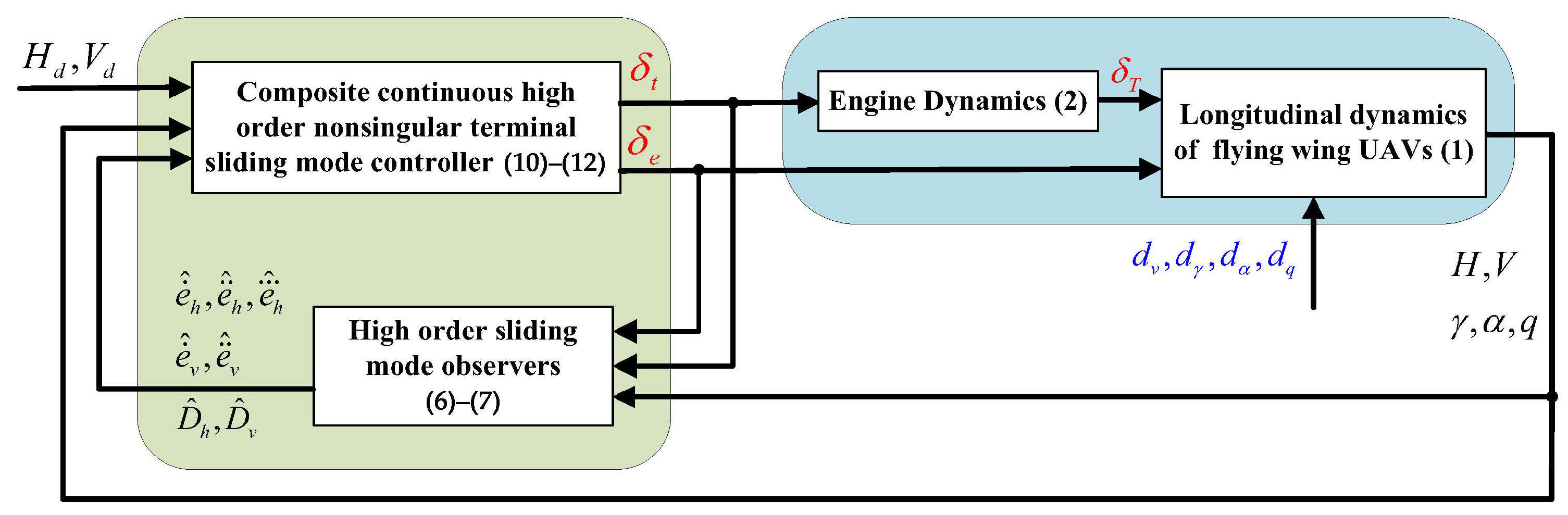
3. Controller Design

In this section, the high-order sliding mode observers (HSMOs) are designed to estimate the derivatives and high-order derivatives of tracking errors and lumped disturbances. Then, based on the estimation information, the composite continuous high-order nonsingular terminal sliding mode controllers (CCNTSMCs) are designed in both altitude and velocity channels.

Assumption 1. 

The lumped disturbances $D_h$ and $D_v$ in the tracking error dynamics (4) are differentiable and their derivatives are bounded and satisfy the following:

$$\left|{\dot{D}}_h\right|\le l_{dh},\left|{\dot{D}}_v\right|\le l_{dv},$$

(5)

where $l_{dh}$ and $l_{dv}$ are positive constants.

3.1. Design of HSMOs

To estimate the derivatives and high-order derivatives of tracking errors and lumped disturbance, HSMOs are designed for the tracking error dynamics (4) as follows:

$$\left\{\begin{array}{c}{v}_h^1=-8l_{oh}^{1/5}{\left|z_h^1-e_h\right|}^{4/5}\mathrm{sign}\left(z_h^1-e_h\right)+z_h^2,\hfill \\ v_h^2=-5l_{oh}^{1/4}{\left|z_h^2-v_h^1\right|}^{3/4}\mathrm{sign}\left(z_h^2-v_h^1\right)+z_h^3,\hfill \\ v_h^3=-3l_{oh}^{1/3}{\left|z_h^3-v_h^2\right|}^{2/3}\mathrm{sign}\left(z_h^3-v_h^2\right)+z_h^4,\hfill \\ v_h^4=-1.5l_{oh}^{1/2}{\left|z_h^4-v_h^3\right|}^{1/2}\mathrm{sign}\left(z_h^4-v_h^3\right)+z_h^5,\hfill \\ {\dot{z}}_h^1=v_h^1,{\dot{z}}_h^2=v_h^2,{\dot{z}}_h^3=v_h^3,\hfill \\ {\dot{z}}_h^4=f_1\left(x\right)+g_1^1\left(x\right){\delta }_e+g_1^2\left(x\right){\delta }_t+v_h^4,\hfill \\ {\dot{z}}_h^5=-1.1l_{oh}\mathrm{sign}\left(z_h^5-v_h^4\right),\hfill \\ {\widehat{\dot{e}}}_h=z_h^2,{\widehat{\ddot{e}}}_h=z_h^3,\widehat{\stackrel{⃛}{e_h}}=z_h^4,{\widehat{D}}_h=z_h^5,\hfill \end{array}\right.$$

(6)

$$\left\{\begin{array}{c}{v}_v^1=-5l_{ov}^{1/4}{\left|z_v^1-e_v\right|}^{3/4}\mathrm{sign}\left(z_v^1-e_v\right)+z_v^2,\hfill \\ v_v^2=-3l_{ov}^{1/3}{\left|z_v^2-v_v^1\right|}^{2/3}\mathrm{sign}\left(z_v^2-v_v^1\right)+z_v^3,\hfill \\ v_v^3=-1.5l_{ov}^{1/2}{\left|z_v^3-v_v^2\right|}^{1/2}\mathrm{sign}\left(z_v^3-v_v^2\right)+z_v^4,\hfill \\ {\dot{z}}_v^1=v_v^1,{\dot{z}}_v^2=v_v^2,\hfill \\ {\dot{z}}_v^3=f_2\left(x\right)+g_2^1\left(x\right){\delta }_e+g_2^2\left(x\right){\delta }_t+v_v^3,\hfill \\ {\dot{z}}_v^4=-1.1l_{ov}\mathrm{sign}\left(z_v^4-v_v^3\right),\hfill \\ {\widehat{\dot{e}}}_v=z_v^2,{\widehat{\ddot{e}}}_v=z_v^3,{\widehat{D}}_v=z_v^4,\hfill \end{array}\right.$$

(7)

where $l_{oh}$ and $l_{ov}$ are sliding mode observer gains which satisfy $l_{oh}\ge l_{dh}$, $l_{ov}\ge l_{dv}$; and $v_h^1\cdots v_h^4$, $z_h^1\cdots z_h^5$, $v_v^1\cdots v_v^3$, and $z_v^1\cdots z_v^4$ are the dynamical states of HSMOs. ${\widehat{e}}_h$, ${\widehat{\ddot{e}}}_h$, $\widehat{\stackrel{⃛}{e_h}}$, ${\widehat{e}}_v$, and ${\widehat{\ddot{e}}}_v$ are the estimations of the altitude and velocity tracking error dynamics; and ${\widehat{D}}_h$ and ${\widehat{D}}_v$ are the estimation of lumped disturbances. The estimation error of HSMOs is defined as follows:

$$\begin{array}{cc}{e}_{{\dot{e}}_h}\hfill & ={\widehat{\dot{e}}}_h-{\dot{e}}_h,e_{{\ddot{e}}_h}={\widehat{\ddot{e}}}_h-{\ddot{e}}_h,e_{\stackrel{⃛}{e_h}}=\widehat{\stackrel{⃛}{e_h}}-\stackrel{⃛}{e_h},e_{D_h}={\widehat{D}}_h-D_h;\hfill \\ e_{{\dot{e}}_v}\hfill & ={\widehat{\dot{e}}}_v-{\dot{e}}_v,e_{{\ddot{e}}_v}={\widehat{\ddot{e}}}_v-{\ddot{e}}_v,e_{D_v}={\widehat{D}}_v-D_v.\hfill \end{array}$$

(8)

According to the theorem in [27], the estimation errors $e_{{\dot{e}}_h}$, $e_{{\ddot{e}}_h}$, $e_{\stackrel{⃛}{e_h}}$, $e_{{\dot{e}}_v}$, $e_{{\ddot{e}}_v}$, $e_{D_h}$, and $e_{D_v}$ converge to zero in finite time, which means the estimation of tracking error dynamics and lumped disturbances converge to their real values in finite time.

Remark 1. 

In the presence of measurement noises, the estimation accuracy of HSMOs (6) and (7) inevitably deteriorates. Assuming the noise magnitude of $e_h$ and $e_v$ is ${ϵ}_h$ and ${ϵ}_v$, respectively, the best possible accuracy of the estimation is as follows:

$$\begin{array}{cc}|e_{{\dot{e}}_h}|\hfill & \le k_1^h{\left(l_{oh}{ϵ}_h\right)}^{{\displaystyle \frac{5}{6}}},|e_{{\ddot{e}}_h}|\le k_2^h{\left(l_{oh}{ϵ}_h\right)}^{{\displaystyle \frac{2}{3}}},|e_{\stackrel{⃛}{e_h}}|\le k_3^h{\left(l_{oh}{ϵ}_h\right)}^{{\displaystyle \frac{4}{2}}},\left|e_{D_h}\right|=\le k_4^h{\left(l_{oh}{ϵ}_h\right)}^{{\displaystyle \frac{1}{3}}};\hfill \\ |e_{{\dot{e}}_v}|\hfill & \le k_1^v{\left(l_{ov}{ϵ}_v\right)}^{{\displaystyle \frac{4}{5}}},|e_{{\ddot{e}}_v}|\le k_2^v{\left(l_{ov}{ϵ}_v\right)}^{{\displaystyle \frac{3}{5}}},\left|e_{D_v}\right|\le k_3^v{\left(l_{ov}{ϵ}_v\right)}^{{\displaystyle \frac{2}{5}}}.\hfill \end{array}$$

where $k_1^h$, $k_2^h$, $k_3^h$, $k_4^h$, $k_1^v$, $k_2^v$, and $k_3^v$ are positive constants.

3.2. Design of CNTSMC

The high-order NTSM manifold is designed as follows:

$$\begin{array}{cc}{s}_h=\hfill & f_1+\widehat{D_h}+g_1^1{\delta }_e+g_1^2{\delta }_t+c_h^0\mathrm{sign}\left(e_h\right){\left|e_h\right|}^{a_h^0}\hfill \\ & +c_h^1\mathrm{sign}\left({\widehat{\dot{e}}}_h\right){\left|{\widehat{\dot{e}}}_h\right|}^{a_h^1}+c_h^2\mathrm{sign}\left({\widehat{\ddot{e}}}_h\right){\left|{\widehat{\ddot{e}}}_h\right|}^{a_h^2}+c_h^3\mathrm{sign}\left(\widehat{\stackrel{⃛}{e_h}}\right){\left|\widehat{\stackrel{⃛}{e_h}}\right|}^{a_h^3},\hfill \\ s_v=\hfill & f_2+\widehat{D_v}+g_2^1{\delta }_e+g_2^2{\delta }_t+c_v^0\mathrm{sign}\left(e_v\right){\left|e_v\right|}^{a_v^0}+c_v^1\mathrm{sign}\left({\widehat{\dot{e}}}_v\right){\left|{\widehat{\dot{e}}}_v\right|}^{a_v^1}+c_v^2\mathrm{sign}\left({\widehat{\ddot{e}}}_v\right){\left|{\widehat{\ddot{e}}}_v\right|}^{a_v^2},\hfill \end{array}$$

(9)

Theorem 1. 

For the longitudinal tracking error dynamics of flying wing UAVs (4), if Assumption 1 is satisfied and the system is in the absence of measurement noise, the composite continuous high-order nonsingular terminal sliding mode controllers

$$\left[\begin{array}{c}{\delta }_e\\ {\delta }_t\end{array}\right]=-{\left[\begin{array}{cc}{g}_1^1& g_1^2\\ g_2^1& g_2^2\end{array}\right]}^{-1}\left[\begin{array}{c}{u}_h^{eq}-u_h^n\\ u_v^{eq}-u_v^n\end{array}\right],$$

(10)

$$\left\{\begin{array}{cc}{u}_h^{eq}=\hfill & c_h^0\mathrm{sign}\left(e_h\right){\left|e_h\right|}^{{\alpha }_h^0}+c_h^1\mathrm{sign}\left({\widehat{\dot{e}}}_h\right){\left|{\widehat{\dot{e}}}_h\right|}^{{\alpha }_h^1}+c_h^2\mathrm{sign}\left({\widehat{\ddot{e}}}_h\right){\left|{\widehat{\ddot{e}}}_h\right|}^{{\alpha }_h^2}+c_h^3\mathrm{sign}\left(\widehat{\stackrel{⃛}{e_h}}\right){\left|\widehat{\stackrel{⃛}{e_h}}\right|}^{{\alpha }_h^3}\hfill \\ & +f_1\left(x\right)+\widehat{D_h},\hfill \\ u_v^{eq}=\hfill & c_v^0\mathrm{sign}\left(e_v\right){\left|e_v\right|}^{{\alpha }_v^0}+c_v^1\mathrm{sign}\left({\widehat{\dot{e}}}_v\right){\left|{\widehat{\dot{e}}}_v\right|}^{{\alpha }_v^1}+c_v^2\mathrm{sign}\left({\widehat{\ddot{e}}}_v\right){\left|{\widehat{\ddot{e}}}_v\right|}^{{\alpha }_v^2}+f_2\left(x\right)+\widehat{D_v},\hfill \end{array}\right.$$

(11)

$$\begin{array}{c}{\dot{u}}_h^n=-{\eta }_h\mathrm{sign}\left(s_h\right),{\dot{u}}_v^n=-{\eta }_v\mathrm{sign}\left(s_v\right),\hfill \end{array}$$

(12)

guarantee the altitude and velocity tracking errors $e_h$, $e_v$ converges to zero in finite time, where ${\eta }_h$ and ${\eta }_v$ are positive constants, and $\widehat{D_h}$ and $\widehat{D_v}$ are acquired by HSMOs (6) and (7). $c_h^0$, $c_h^1$, $c_h^2$, $c_h^3$, $c_v^0$, $c_v^1$, and $c_v^2$ are positive constants and satisfy that the polynomial $s^5+c_h^4{s}^4+c_h^3{s}^3+c_h^2{s}^2+c_h^{1}s+c_h^0$ and $s^4+c_v^3{s}^3+c_v^2{s}^2+c_v^{1}s+c_v^0$ are Hurwitz stable. ${\alpha }_h^0$, ${\alpha }_h^1$, ${\alpha }_h^2$, ${\alpha }_h^3$, ${\alpha }_v^0$, ${\alpha }_v^1$, and ${\alpha }_v^2$ are positive constants and satisfy the following:

$$\begin{array}{c}{\alpha }_h^{i-1}={\displaystyle \frac{{\alpha }_h^i{\alpha }_h^{i+1}}{2{\alpha }_h^{i+1}-{\alpha }_h^i}},i=1,2,3,{\alpha }_v^{j-1}={\displaystyle \frac{{\alpha }_v^j{\alpha }_v^{j+1}}{2{\alpha }_v^{j+1}-{\alpha }_v^j}},j=1,2,\hfill \end{array}$$

(13)

with ${\alpha }_h^4=1$, ${\alpha }_h^3\in \left(0,1\right)$; ${\alpha }_v^3=1$, ${\alpha }_v^2\in \left(0,1\right)$.

The control structure of the proposed composite continuous high-order nonsingular terminal sliding mode controllers for the flying wing UAVs is given in Figure 1.

Remark 2. 

The proposed controller consists of Equations (6), (7), and (9)–(12), which contain many exponential operations, thus posing a significant burden and making it difficult to implement on basic flight control hardware such as the STM32 or PX4. With the continuous development of hardware technology, especially the rapid advancement of flight control board chips, the proposed method holds great promise for implementation in future flight hardware.

4. Stability Analysis

Considering the fact that the tracking error dynamics of altitude and velocity (4) and controllers (10)–(12) have the same form, it is only necessary to analyze the stability of one channel, without loss of generality, and we choose the altitude channel as an example.

Proof of Theorem 1. 

The proof of Theorem 1 can be divided into the following three steps:

(1) 

Finite-time convergence of the sliding variable

Substituting the controller (10)–(12) into the sliding manifold (9) yields the following:

$$s_h=u_h^n.$$

(14)

Taking the derivative of Equation (14) along with Equation (12) acquires the following:

$${\dot{s}}_h=-{\eta }_h\mathrm{sign}\left(s_h\right).$$

(15)

A Lyapunov function in terms of $s_h$ is chosen as follows:

$$\begin{array}{c}{V}_s={\displaystyle \frac{1}{2}}{s_h}^2.\hfill \end{array}$$

(16)

The derivative of $V_s$ along with Equation (15) is taken, and we obtain

$$\begin{array}{c}{\dot{V}}_s=-{\eta }_h\left|s_h\right|=-\sqrt{2}{\eta }_h{V_s}^{1/2}.\hfill \end{array}$$

(17)

It can be obtained from Equation (17) that

$$\begin{array}{c}{V}_s^{1/2}\left(t\right)=V_s^{1/2}\left(0\right)-{\displaystyle \frac{\sqrt{2}}{2}}{\eta }_{h}t.\hfill \end{array}$$

(18)

Considering ${\eta }_h$ is a positive constant, $V_s\left(t\right)$ converges to zero in finite time, and this denotes that the sliding variable $s_h$ converges to zero in finite time.

(2) 

Finite-time boundness of system states

With Equation (14) in mind, substituting Equations (10)–(12) into Equation (4) yields the following:

$$\begin{array}{cc}{e}_h^{\left(4\right)}=\hfill & -e_{D_h}-c_h^0\mathrm{sign}\left(e_h\right){\left|e_h\right|}^{{\alpha }_h^0}-c_h^1\mathrm{sign}\left({\widehat{\dot{e}}}_h\right){\left|{\widehat{\dot{e}}}_h\right|}^{{\alpha }_h^1}-c_h^2\mathrm{sign}\left({\widehat{\ddot{e}}}_h\right){\left|{\widehat{\ddot{e}}}_h\right|}^{{\alpha }_h^2}\hfill \\ & -c_h^3\mathrm{sign}\left(\widehat{\stackrel{⃛}{e_h}}\right){\left|\widehat{\stackrel{⃛}{e_h}}\right|}^{{\alpha }_h^3}+s_h.\hfill \end{array}$$

(19)

A Lyapunov function is chosen in terms of $s_h$, $e_h$, ${\dot{e}}_h$, ${\ddot{e}}_h$, and $\stackrel{⃛}{e_h}$ as follows:

$$\begin{array}{c}{V}_B={\displaystyle \frac{1}{2}}\left[{s_h}^2+{e_h}^2+{{\dot{e}}_h}^2+{{\ddot{e}}_h}^2+{\left(\stackrel{⃛}{e_h}\right)}^2\right].\hfill \end{array}$$

(20)

Considering Equations (8) and (19), the derivative of $V_B$ is taken, and we have

$$\begin{array}{cc}{\dot{V}}_B\hfill & =s_h{\dot{s}}_h+e_h{\dot{e}}_h+{\dot{e}}_h{\ddot{e}}_h+{\ddot{e}}_h\stackrel{⃛}{e_h}+\stackrel{⃛}{e_h}{e}_h^{\left(4\right)}\hfill \\ & =-{\eta }_h\left|s_h\right|+e_h{\dot{e}}_h+{\dot{e}}_h{\ddot{e}}_h+{\ddot{e}}_h\stackrel{⃛}{e_h}+\left|\stackrel{⃛}{e_h}{s}_h\right|-\stackrel{⃛}{e_h}\left[c_h^0\mathrm{sign}\left(e_h\right){\left|e_h\right|}^{{\alpha }_h^0}\right.+c_h^1\mathrm{sign}\left({\widehat{\dot{e}}}_h\right){\left|{\widehat{\dot{e}}}_h\right|}^{{\alpha }_h^1}\hfill \\ & +c_h^2\mathrm{sign}\left({\widehat{\ddot{e}}}_h\right){\left|{\widehat{\ddot{e}}}_h\right|}^{{\alpha }_h^2}+c_h^3\mathrm{sign}\left(\widehat{\stackrel{⃛}{e_h}}\right){\left|\widehat{\stackrel{⃛}{e_h}}\right|}^{{\alpha }_h^3}\left.+e_{D_h}\right]\hfill \\ & \le \left|e_h{\dot{e}}_h\right|+\left|{\dot{e}}_h{\ddot{e}}_h\right|+\left|{\ddot{e}}_h\stackrel{⃛}{e_h}\right|+\left|\stackrel{⃛}{e_h}{s}_h\right|+c_h^0\left|\stackrel{⃛}{e_h}·{\left(e_h\right)}^{{\alpha }_h^0}\right|+c_h^1\left|\stackrel{⃛}{e_h}·{\left({\dot{e}}_h+e_{{\dot{e}}_h}\right)}^{{\alpha }_h^1}\right|\hfill \\ & +c_h^2\left|\stackrel{⃛}{e_h}·{\left({\ddot{e}}_h+e_{{\ddot{e}}_h}\right)}^{{\alpha }_h^2}\right|+c_h^3\left|\stackrel{⃛}{e_h}·{\left(\stackrel{⃛}{e_h}+e_{\stackrel{⃛}{e_h}}\right)}^{{\alpha }_h^3}\right|+\left|\stackrel{⃛}{e_h}{e}_{D_h}\right|.\hfill \end{array}$$

(21)

Note that, for arbitrary variable x, if $0<\alpha <1$, it can be verified that

$$\begin{array}{c}{\left|x\right|}^{\alpha }\le 1+\alpha \left|x\right|\le 1+\left|x\right|.\hfill \end{array}$$

(22)

Therefore, we have

$$\begin{array}{c}{\left|e_h\right|}^{{\alpha }_h^0}\le 1+\left|e_h\right|,{\left|{\dot{e}}_h\right|}^{{\alpha }_h^1}\le 1+\left|{\dot{e}}_h\right|,{\left|{\ddot{e}}_h\right|}^{{\alpha }_h^2}\le 1+\left|{\ddot{e}}_h\right|,{\left|\stackrel{⃛}{e_h}\right|}^{{\alpha }_h^3}\le 1+\left|\stackrel{⃛}{e_h}\right|.\hfill \end{array}$$

(23)

Substituting Equation (23) into Equation (21) acquires the following:

$$\begin{array}{cc}{\dot{V}}_B\hfill & \le \left|e_h{\dot{e}}_h\right|+\left|{\dot{e}}_h{\ddot{e}}_h\right|+\left|{\ddot{e}}_h\stackrel{⃛}{e_h}\right|+\left|\stackrel{⃛}{e_h}{e}_{D_h}\right|+\left|\stackrel{⃛}{e_h}{s}_h\right|+\left(c_h^0+c_h^1+c_h^2+c_h^3\right)\left|\stackrel{⃛}{e_h}\right|+c_h^0\left|\stackrel{⃛}{e_h}s{e}_h\right|\hfill \\ & +c_h^1\left|\stackrel{⃛}{e_h}{\dot{e}}_h\right|+c_h^1\left|\stackrel{⃛}{e_h}{e}_{{\dot{e}}_h}\right|+c_h^2\left|\stackrel{⃛}{e_h}{\ddot{e}}_h\right|+c_h^2\left|\stackrel{⃛}{e_h}{e}_{{\ddot{e}}_h}\right|+c_h^3\left|\stackrel{⃛}{e_h}\right|+c_h^3\left|\stackrel{⃛}{e_h}{e}_{\stackrel{⃛}{e_h}}\right|\hfill \\ & \le {\displaystyle \frac{{e_h}^2+{{\dot{e}}_h}^2}{2}}+{\displaystyle \frac{{{\dot{e}}_h}^2+{{\ddot{e}}_h}^2}{2}}+{\displaystyle \frac{{{\ddot{e}}_h}^2+{\left(\stackrel{⃛}{e_h}\right)}^2}{2}}+{\displaystyle \frac{{s_h}^2+{\left(\stackrel{⃛}{e_h}\right)}^2}{2}}+c_h^0{\displaystyle \frac{{\left(\stackrel{⃛}{e_h}\right)}^2+{e_h}^2}{2}}\hfill \\ & +c_h^1{\displaystyle \frac{{\left(\stackrel{⃛}{e_h}\right)}^2+{{\dot{e}}_h}^2}{2}}+c_h^1{\displaystyle \frac{{\left(\stackrel{⃛}{e_h}\right)}^2+{{\dot{e}}_{{\dot{e}}_h}}^2}{2}}+c_h^2{\displaystyle \frac{{\left(\stackrel{⃛}{e_h}\right)}^2+{{\ddot{e}}_h}^2}{2}}+c_h^2{\displaystyle \frac{{\left(\stackrel{⃛}{e_h}\right)}^2+{e_{{\ddot{e}}_h}}^2}{2}}\hfill \\ & +c_h^2{\left(\stackrel{⃛}{e_h}\right)}^2+c_h^3{\displaystyle \frac{{\left(\stackrel{⃛}{e_h}\right)}^2+{\left(e_{\stackrel{⃛}{e_h}}\right)}^2}{2}}+{\displaystyle \frac{{\left(\stackrel{⃛}{e_h}\right)}^2+{e_{D_h}}^2}{2}}+{\displaystyle \frac{{\left(\stackrel{⃛}{e_h}\right)}^2+{e_{D_h}}^2}{2}}\hfill \\ & +\left(c_h^0+c_h^1+c_h^2+c_h^3\right){\displaystyle \frac{1+2{\left(\stackrel{⃛}{e_h}\right)}^2}{2}}\hfill \\ & \le \left[{\displaystyle \frac{5}{2}}+{\displaystyle \frac{3}{2}}\left(c_h^0+c_h^1+c_h^2+c_h^3\right)\right]V_B\hfill \\ & +{\displaystyle \frac{1}{2}}\left(c_h^1{e_{{\dot{e}}_h}}^2+c_h^2{e_{{\ddot{e}}_h}}^2+c_h^3{e_{\stackrel{⃛}{e_h}}}^2\right)+{\displaystyle \frac{1}{2}}\left(c_h^0+c_h^1+c_h^2+c_h^3\right).\hfill \end{array}$$

(24)

The above equation can be rewritten in the following compact form:

$$\begin{array}{c}{\dot{V}}_B<K_B{V}_B+L_B,\hfill \end{array}$$

(25)

with

$$\begin{array}{c}{K}_B={\displaystyle \frac{5}{2}}+{\displaystyle \frac{3}{2}}\left(c_h^0+c_h^1+c_h^2+c_h^3\right),L_B={\displaystyle \frac{1}{2}}\left(c_h^1{e_{{\dot{e}}_h}}^2+c_h^2{e_{{\ddot{e}}_h}}^2+c_h^3{e_{\stackrel{⃛}{e_h}}}^2\right)+{\displaystyle \frac{1}{2}}\left(c_h^0+c_h^1+c_h^2+c_h^3\right).\hfill \end{array}$$

Since $c_h^0$, $c_h^1$, $c_h^2$, and $c_h^3$ are positive constants and $e_{{\dot{e}}_h}$, $e_{{\ddot{e}}_h}$, and $e_{\stackrel{⃛}{e_h}}$ are the estimation errors of HSMOs, $K_B$ and $L_B$ are both positive and bounded. Furthermore, there exist positive constants $K_{B\max }$ and $L_{B\max }$ which satisfy $K_B\le K_{B\max },L_B\le L_{B\max }$, and it can be obtained from Equation (25) that

$$\begin{array}{c}{V}_B\left(t\right)\le \left[V_B\left(0\right)+{\displaystyle \frac{L_{B\max }}{K_{B\max }}}\right]e^{K_{B\max }t}-{\displaystyle \frac{L_{B\max }}{K_{B\max }}}.\hfill \end{array}$$

(26)

Therefore, for any bounded time t, $V_B\left(t\right)$ is bounded, which means the altitude tracking error $e_h$ and its dynamics will not escape to infinity in finite time.

(3) 

Finite-time convergence of tracking error

Since $s_h$ converges to zero in finite time, there exists a bounded constant $t_{s=0}$ such that, when $t\ge t_{s=0}$, the sliding variable $s_h$ is equal to zero. Since HSMOs guarantee that the estimation errors $e_{{\dot{e}}_h}$, $e_{{\ddot{e}}_h}$, and $e_{\stackrel{⃛}{e_h}}$ converge to zero in finite time, there exists a bounded constant $t_{e_o=0}$ which satisfies that, when $t\ge t_{e_o=0}$, the estimation errors are kept as zeros. By definition, $T=\max \left\{t_{s=0},t_{e_o=0}\right\}$ when $t\ge T$, and we have

$$\begin{array}{c}0={e_h}^{\left(4\right)}+c_h^0\mathrm{sign}\left(e_h\right){\left|e_h\right|}^{{\alpha }_h^0}+c_h^1\mathrm{sign}\left({\dot{e}}_h\right){\left|{\dot{e}}_h\right|}^{{\alpha }_h^1}+c_h^2\mathrm{sign}\left({\ddot{e}}_h\right){\left|{\ddot{e}}_h\right|}^{{\alpha }_h^2}+c_h^3\mathrm{sign}\left(\stackrel{⃛}{e_h}\right){\left|\stackrel{⃛}{e_h}\right|}^{{\alpha }_h^3}.\hfill \end{array}$$

(27)

According to the Theorem in [28], the altitude tracking error $e_h\left(t\right)$ converges to zero in finite time, which completes the proof. □

5. Simulation Study

5.1. Simulation Scenario Setting

The tracking performance of the proposed composite continuous high-order nonsingular terminal sliding mode controller is tested in this part through numerical simulations. The traditional method without the high-order sliding mode observer is also employed here as a comparison. The body parameters of the tested flying wing UAV are given in

Table 1. Body parameters of the tested flying wing UAV.

Parameters	${\mathit{I}}_{\mathit{yy}}$	S	c	${\mathit{S}}_{\mathit{p}}$	m
Value	1.135	0.55	0.19	0.20	13.5
Units	kg·m2	m2	m	m2	kg

.

The initial states of the tested flying wing UAV are set as follows:

$$\begin{array}{cccc}X\left(0\right)=0;\hfill & H\left(0\right)=15 \mathrm{m};& V\left(0\right)=25 \mathrm{m}/\mathrm{s};& \gamma \left(0\right)=5^{\circ };\\ \alpha \left(0\right)=0;\hfill & q\left(0\right)=0;\hfill & {\delta }_T\left(0\right)=0.4;\hfill & {\dot{\delta }}_T\left(0\right)=0.\end{array}$$

The velocity command is set as $V_d=25$, and the altitude command is set as follows:

$$H_d=\left\{\begin{array}{cc}15+0.5t,\hfill & t\le 10 \mathrm{s},\hfill \\ 20+2.5\left(t-10\right),\hfill & 10<t\le 50 \mathrm{s},\hfill \\ 120,\hfill & t<65 \mathrm{s}.\hfill \end{array}\right.$$

The UAV is set to suffer external time-varying wind $d_w=3sin\left(t\right)$, and its real velocity in model (1) changes to $V=V_n+d_w$, where $V_n$ is the nominal value of velocity. To make the simulation more challenging, the throttle and elevator are set to suffer the following failures:

(1)

When $t\ge 15$ s, the engine throttle ${\delta }_t$ begins to suffer 20% efficiency loss;

(2)

When $t\ge 35$ s, the elevator ${\delta }_e$ begins to suffer 20% efficiency loss.

To verify the effectiveness of the proposed method, simulations with other methods are also carried out. The tested methods include (1) the proposed composite NTSM control method based on an HSMO (CNTSM + HSMO); (2) a composite NTSM control method based on an ESO (CNTSM + ESO); (3) a composite nonlinear dynamic inversion control method based on an HSMO (CNDI + HSMO); (4) a composite nonlinear dynamic inversion control method based on an extended state observer (CNDI + ESO).

The controller and observer of the proposed method in this paper are designed in the form of Equations (10)–(12) and Equations (6) and (7), respectively, and the parameters of the controller and observer are set as follows:

$$\begin{array}{cc}{\alpha }_h^0=\hfill & {\displaystyle \frac{9}{13}},{\alpha }_h^1={\displaystyle \frac{3}{4}},{\alpha }_h^2={\displaystyle \frac{9}{11}},{\alpha }_h^3={\displaystyle \frac{9}{10}},{\alpha }_v^0={\displaystyle \frac{4}{7}},{\alpha }_v^1={\displaystyle \frac{2}{3}},{\alpha }_v^2={\displaystyle \frac{4}{5}},\hfill \\ c_h^0=\hfill & 16,c_h^1=32,c_h^2=24,c_h^3=8,c_v^0=64,c_v^1=48,c_v^2=12,\hfill \\ {\eta }_h=\hfill & 1,l_{oh}=50{\eta }_v=1,l_{ov}=150.\hfill \end{array}$$

The CNDI controllers are designed as follows:

$$\begin{array}{cc}{u}_h^1\hfill & =k_h^0{e}_h+k_h^1{\widehat{\dot{e}}}_h+k_h^2{\widehat{\ddot{e}}}_h+k_h^3\widehat{\stackrel{⃛}{e_h}},u_v^1=k_v^0{e}_v+k_v^1{\widehat{\dot{e}}}_v+k_v^2{\widehat{\ddot{e}}}_v,\hfill \end{array}$$

$$\begin{array}{c}\left[\begin{array}{c}{\delta }_e\\ {\delta }_t\end{array}\right]=-{\left[\begin{array}{cc}{g}_1^1& g_1^2\\ g_2^1& g_2^2\end{array}\right]}^{-1}\left[\begin{array}{c}{f}_1+{\widehat{D}}_h+u_h^1\\ f_2+{\widehat{D}}_v+u_v^1\end{array}\right].\hfill \end{array}$$

The CNDI control parameters are set as follows:

$$\begin{array}{ccccccc}{k}_h^0=16,& k_h^1=32,& k_h^2=24,& k_h^3=8,& k_v^0=64,& k_v^0=48,& k_v^0=12.\end{array}$$

Taking the altitude channel as an example, the ESO is designed as follows:

$$\begin{array}{c}\left\{\begin{array}{c}{\dot{z}}_1=z_2-l_h^1\left(z_1-e_h\right),\hfill \\ {\dot{z}}_2=z_3-l_h^2\left(z_1-e_h\right),\hfill \\ {\dot{z}}_3=z_4-l_h^3\left(z_1-e_h\right),\hfill \\ {\dot{z}}_4=f_1+g_1^1{\delta }_e+g_1^2{\delta }_t+z_5-l_h^4\left(z_1-e_h\right),\hfill \\ {\dot{z}}_5=-l_h^5\left(z_1-e_h\right),\hfill \\ z_h^2={\widehat{\dot{e}}}_h,z_h^3={\widehat{\ddot{e}}}_h,z_h^4=\widehat{\stackrel{⃛}{e_h}},z_h^5={\widehat{D}}_h.\hfill \end{array}\right.\hfill \end{array}$$

The parameters of the ESO are set as follows:

$$\begin{array}{ccccc}{l}_h^1=100,\hfill & l_h^2=4000,\hfill & l_h^3=\mathrm{80,000},\hfill & l_h^4=\mathrm{800,000},\hfill & l_h^5=\mathrm{3,2000,000}.\hfill \end{array}$$

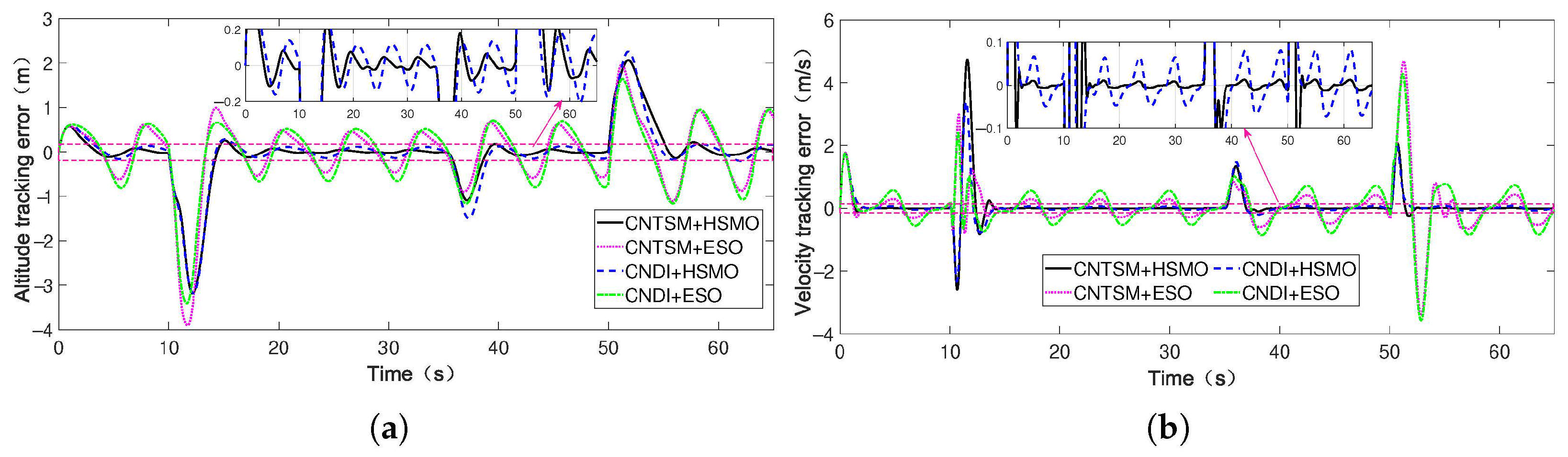
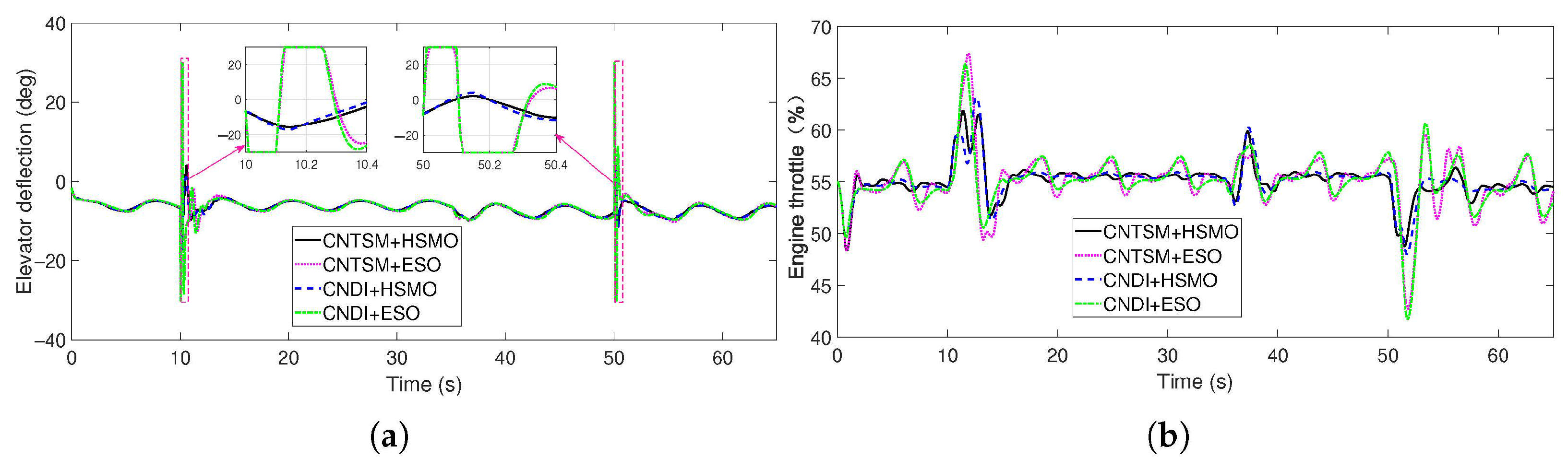
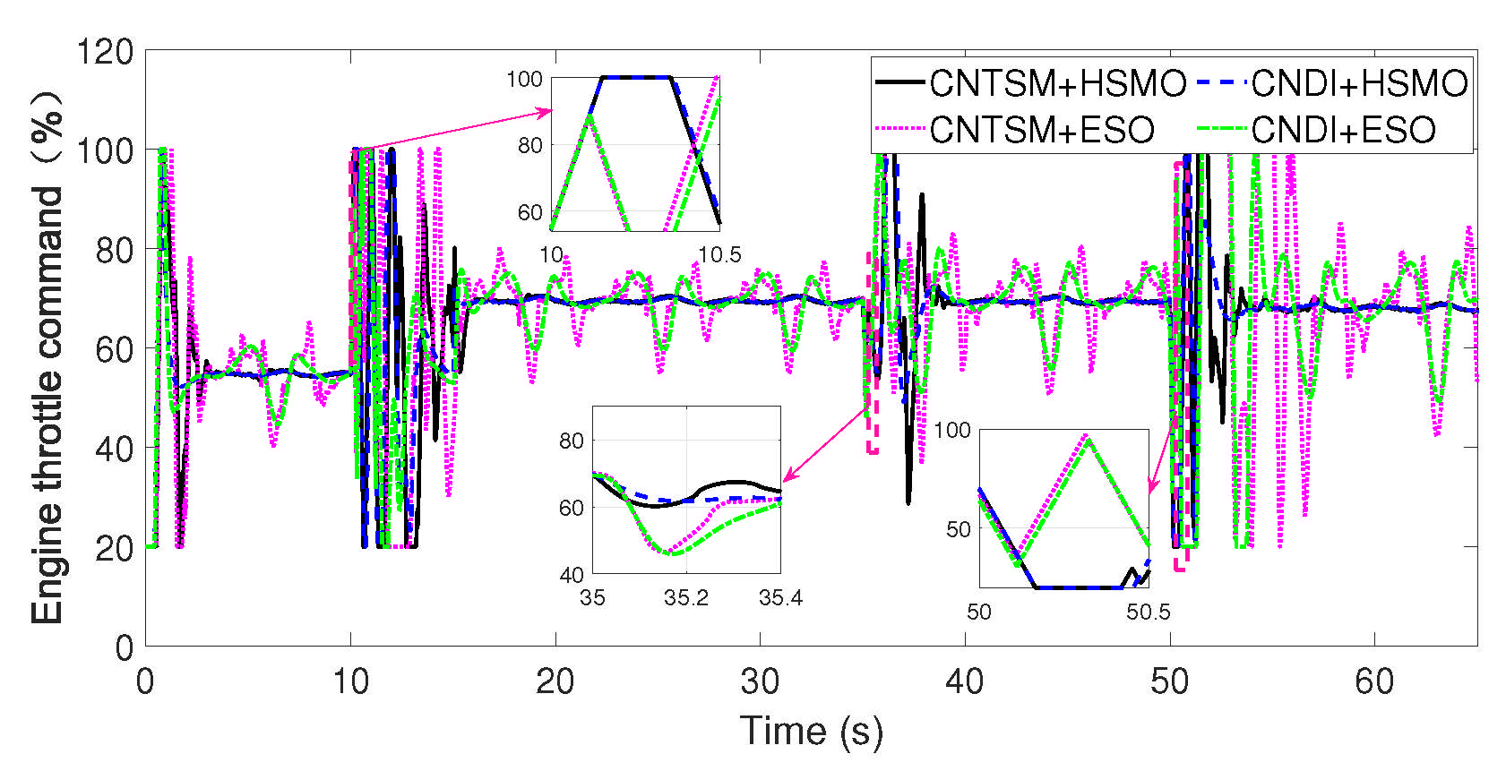
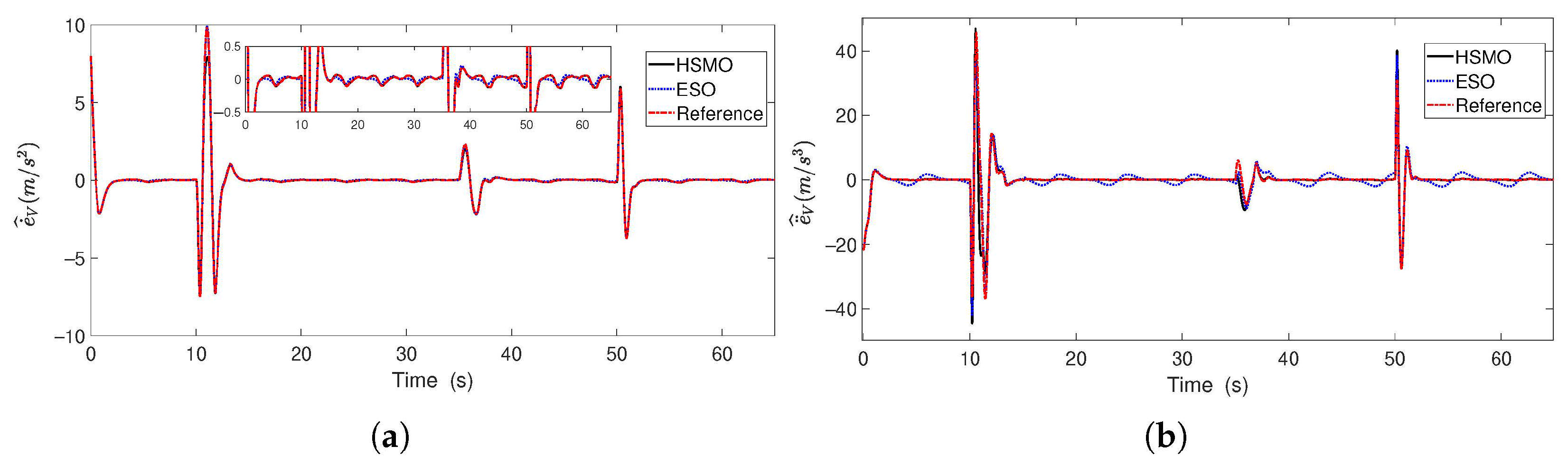
5.2. Simulation Results

The simulation results for the flying wing UAV under the above four control schemes are shown as Figure 2, Figure 3, Figure 4, Figure 5 and Figure 6. Figure 2 demonstrates the response to altitude and velocity tracking errors. It can be seen from Figure 2 that the CNDI + ESO method has the worst tracking performance among the four methods, which means that the HSMO-based composite method has better tracking performance than the ESO-based method. Although CNTSM + HSMO and CNDI + HSMO both achieve good tracking performance, it can be observed from the zoomed-in figures in Figure 2 that the proposed CNTSM + HSMO method has a better tracking performance in terms of the following two aspects: (1) convergence speed, where the proposed method guarantees the altitude and velocity tracking errors converge to zero faster than the CNDI + HSMO, especially when the velocity command changes sharply (i.e., $t=15$ s) or the UAV suffers serious actuator faults (i.e., $t=35$ s); and (2) steady-state tracking errors, where it can be observed from the zoomed-in figures in Figure 2 that the convergence bound of the proposed method is smaller than that of the CNDI + HSMO method.

Figure 3a,b and Figure 4 show the response curves of elevator deflection, the throttle of the flying wing UAVs, and the throttle command of the engine, respectively. As shown by Figure 3a and Figure 4, the elevator deflection and engine throttle command change sharply when the altitude command of the UAV changes at 10 s and 50 s. It also can observed from the zoomed-in figures in Figure 3 that the control actions of the four methods are all continuous. Figure 3b shows the response of the engine throttle, and it can be seen that the real engine throttle changes smoothly and its changing trend is similar with the engine throttle command.

Figure 5 and Figure 6 demonstrate the estimation performance of the HSMO and ESO. It can be clearly observed from the zoomed-in figures in Figure 5 and Figure 6 that the HSMO method achieves a higher-precision estimation than the ESO.

6. Conclusions

This study proposes a continuous composite nonsingular terminal sliding mode control method for the longitudinal command tracking control problem of flying wing UAVs with multi-source disturbances and actuator faults. The proposed method not only guarantees the finite-time convergence of tracking errors but also guarantees the continuity of control action. Simulation results validate that the proposed method achieves good tracking of altitude and velocity even when there exist serious disturbances and actuator faults in the flying wing UAV’s system.

Due to the significant influence of measurement noise on the flight control system [29] and high-order sliding mode observer [30], we will perform a robust analysis of the flight control system with disturbance and measurement noise. Additionally, many novel sliding mode methods have been designed to deal with practical problems such as actuator attacks [31], batch processes [32], and human–robot interaction [33], and we will try to use these novel methods in the controller design of flying wing UAVs in future research.

References

1. Xu, X.; Zhou, Z. Study on longitudinal stability improvement of flying wing aircraft based on synthetic jet flow control. Aerosp. Sci. Technol. 2015, 46, 287–298. [Google Scholar] [CrossRef]
2. Wu, W.; Wang, Y.; Gong, C.; Ma, D. Path following control for miniature fixed-wing unmanned aerial vehicles under uncertainties and disturbances a two-layered framework. Nonlinear Dyn. 2022, 108, 3761–3781. [Google Scholar] [CrossRef]
3. Zhao, Z.; Cao, D.; Yang, J.; Wang, H. High-order sliding mode observer-based trajectory tracking control for a quadrotor UAV with uncertain dynamics. Nonlinear Dyn. 2020, 102, 2583–2596. [Google Scholar] [CrossRef]
4. Qu, X.; Zhang, W.; Shi, J.; Lyu, Y. A novel yaw control method for flying wing aircraft in low velocity regime. Aerosp. Sci. Technol. 2017, 69, 636–649. [Google Scholar] [CrossRef]
5. Zhang, S.; Meng, Q. An anti-windup INDI fault-tolerant control scheme for flying wing aircraft with actuator faults. ISA Trans. 2019, 93, 172–179. [Google Scholar] [CrossRef]
6. Li, J.-G.; Chen, X.; Li, Y.-J.; Zhang, R. Control system design of flying wing UAV based on nonlinear methodology. Def. Technol. 2017, 13, 397–405. [Google Scholar] [CrossRef]
7. Wang, X.; Sun, S.; Tao, C.; Xu, B. Neural sliding mode control of low-altitude flying UAV considering wave effect. Comput. Electr. Eng. 2017, 96, 107505. [Google Scholar] [CrossRef]
8. Mei, K.; Ding, S.; Yu, X. A generalized supertwisting algorithm. IEEE Trans. Syst. Man Cybern Cybern. 2022, 53, 3951–3960. [Google Scholar] [CrossRef]
9. Ding, S.; Zhang, B.; Mei, K.; Park, J.H. Adaptive fuzzy SOSM controller design with output constraints. IEEE Trans. Fuzzy Syst. 2022, 30, 2300–2311. [Google Scholar] [CrossRef]
10. Feng, Y.; Yu, X.H.; Man, Z.H. Non-singular terminal sliding mode control of rigid manipulators. Automatica 2002, 38, 2159–2167. [Google Scholar] [CrossRef]
11. Zhao, Z.; Yang, J.; Li, S.; Yu, X.; Wang, Z. Continuous output feedback TSM control for uncertain systems with a DC-AC inverter example. IEEE Trans. Circuits-II 2017, 65, 71–75. [Google Scholar] [CrossRef]
12. Lian, S.; Meng, W.; Lin, Z.; Shao, K.; Zheng, J.; Li, H.; Lu, R. Adaptive attitude control of a quadrotor using fast nonsingular terminal sliding mode. IEEE Trans. Ind. Electron. 2022, 69, 1597–1607. [Google Scholar] [CrossRef]
13. Dong, R.Q.; Wu, A.G.; Zhang, Y. Anti-unwinding sliding mode attitude maneuver control for rigid spacecraft. IEEE Trans. Autom. Control 2022, 67, 978–985. [Google Scholar] [CrossRef]
14. Man, Z.H.; Paplinski, A.P.; Wu, H.R. A robust MIMO terminal sliding mode control scheme for rigid robotic manipulators. IEEE Trans. Autom. Control 1994, 39, 2464–2469. [Google Scholar]
15. Yang, J.; Li, S.H.; Su, J.; Yu, X. Continuous nonsingular terminal sliding mode control for systems with mismatched disturbances. Automatica 2013, 49, 2287–2291. [Google Scholar] [CrossRef]
16. Han, J. From PID to active disturbance rejection control. IEEE Trans. Ind. Electron. 2009, 56, 900–906. [Google Scholar] [CrossRef]
17. Wang, Z.J.; Wang, T. Based on robust sliding mode and linear active disturbance rejection control for attitude of quadrotor load UAV. Nonlinear Dyn. 2022, 108, 3485–3503. [Google Scholar] [CrossRef]
18. Wang, R.; Zhou, Z.; Zhu, X.P.; Wang, Z. Responses and suppression of Joined-Wing UAV in wind field based on distributed model and active disturbance rejection control. Aerosp. Sci. Technol. 2021, 115, 106803. [Google Scholar] [CrossRef]
19. Yu, X.; Yang, J.; Li, S.H. Disturbance observer-based autonomous landing control of unmanned helicopters on moving shipboard. Nonlinear Dyn. 2020, 102, 131–150. [Google Scholar] [CrossRef]
20. Hao, W.; Xian, B.; Xie, T. Fault-tolerant position tracking control design for a tilt tri-rotor unmanned aerial vehicle. IEEE Trans. Ind. Electron. 2022, 69, 604–612. [Google Scholar] [CrossRef]
21. Avram, R.C.; Zhang, X.; Muse, J. Nonlinear adaptive fault-tolerant quadrotor altitude and attitude tracking with multiple actuator faults. IEEE Trans. Control Syst. Technol. 2018, 26, 701–707. [Google Scholar] [CrossRef]
22. Zhang, S.; Shuang, W.; Meng, Q. Control surface faults neural adaptive compensation control for tailless flying wing aircraft with uncertainties. Int. J. Control Autom. Syst. 2018, 16, 1660–1669. [Google Scholar] [CrossRef]
23. Yan, K.; Chen, M.; Wu, Q.; Jiang, B. Extended state observer-based sliding mode fault-tolerant control for unmanned autonomous helicopter with wind gusts. IET Control Theory A 2019, 13, 1500–1513. [Google Scholar] [CrossRef]
24. Mulgund, S.S.; Stengel, R.F. Optimal nonlinear estimation for aircraft flight control in wind shea. Automatica 1996, 32, 3–13. [Google Scholar] [CrossRef]
25. Liu, C.J.; Chen, W.H. Disturbance rejection flight control for small fixed-wing unmanned aerial vehicles. J. Guid. Control Dyn. 2016, 39, 2804–2813. [Google Scholar] [CrossRef]
26. Wang, Q.; Stengel, R.F. Robust nonlinear control of a hypersonic aircraft. J. Guid. Control Dyn. 2000, 23, 577–585. [Google Scholar] [CrossRef]
27. Levant, A. Higher-order sliding modes, differentiation and output-feedback control. Int. J. Control 2003, 76, 924–941. [Google Scholar] [CrossRef]
28. Bhat, S.P.; Bernstein, D.S. Geometric homogeneity with applications to finite-time stability. Math. Control Signals Syst. 2005, 17, 101–127. [Google Scholar] [CrossRef]
29. Li, T.; Zhao, Z.; Ding, S.; Su, J. Composite controller design for quadrotor UAVs with uncertainties and noises based on combined Kalman filter and GPIO. IEEE Trans. Aerosp. Electron. Syst. 2024, 60, 882–892. [Google Scholar] [CrossRef]
30. Levant, A. Robust exact differentiation via sliding mode technique. Automatica 1998, 34, 379–384. [Google Scholar] [CrossRef]
31. Wang, J.; Zheng, Y.; Ding, J.; Xie, X.; Zhang, W. Multiasynchronous extended dissipative sliding mode control of LC circuits in grid-connected system under actuator attacks. IEEE Trans. Circuits Syst. I 2025, 72, 1609–1620. [Google Scholar] [CrossRef]
32. Shi, H.; Gao, W.; Jiang, X.; Su, C.; Li, P. Two-dimensional model-free Q-learning-based output feedback fault-tolerant control for batch processes. Comput. Chem. Eng. 2024, 182, 108583. [Google Scholar] [CrossRef]
33. Liang, X.; Yan, Y.; Wang, W.; Su, T.; He, G.; Li, G.; Hou, Z.-G. Adaptive human–robot interaction torque estimation with high accuracy and strong tracking ability for a lower limb rehabilitation robot. IEEE-ASME Trans. Mechatron. 2024, 29, 4814–4825. [Google Scholar] [CrossRef]
Figure 1. Control structure of the proposed composite continuous finite-time controllers for flying wing UAVs.
Mathematics 13 02375 g001
Figure 2. Response of tracking errors: (a) altitude tracking error; (b) velocity tracking error.
Mathematics 13 02375 g002
Figure 3. Response of control action: (a) elevator deflection angle; (b) engine throttle command.
Mathematics 13 02375 g003
Figure 4. Response of engine throttle command.
Mathematics 13 02375 g004
Figure 5. Response curves of the estimation performance in the altitude channel: (a) e ˙ H and its estimation; (b) e ¨ H and its estimation.
Mathematics 13 02375 g005
Figure 6. Response curves of the estimation performance in the velocity channel: (a) e ˙ v and its estimation; (b) e ¨ v and its estimation.
Mathematics 13 02375 g006