Newly Formulated General Solutions for the Navier Equation in Linear Elasticity

Abstract

The Navier equations are reformulated to be third-order partial differential equations. New anti-Cauchy-Riemann equations can express a general solution in 2D space for incompressible materials. Based on the third-order solutions in 3D space and the Boussinesq–Galerkin method, a third-order method of fundamental solutions (MFS) is developed. For the 3D Navier equation in linear elasticity, we present three new general solutions, which have appeared in the literature for the first time, to signify the theoretical contributions of the present paper. The first one is in terms of a biharmonic function and a harmonic function. The completeness of the proposed general solution is proven by using the solvability conditions of the equations obtained by equating the proposed general solution to the Boussinesq–Galerkin solution. The second general solution is expressed in terms of a harmonic vector, which is simpler than the Slobodianskii general solution, and the traditional MFS. The main achievement is that the general solution is complete, and the number of harmonic functions, three, is minimal. The third general solution is presented by a harmonic vector and a biharmonic vector, which are subjected to a constraint equation. We derive a specific solution by setting the two vectors in the third general solution as the vectorizations of a single harmonic potential. Hence, we have a simple approach to the Slobodianskii general solution. The applications of the new solutions are demonstrated. Owing to the minimality of the harmonic functions, the resulting bases generated from the new general solution are complete and linearly independent. Numerical instability can be avoided by using the new bases. To explore the efficiency and accuracy of the proposed MFS variant methods, some examples are tested.

1. Introduction

The Navier equation, not considering body force, is [1]:

$$G\Delta \mathbf{u}+{\displaystyle \frac{G}{1-2\nu }}\nabla (\nabla ·\mathbf{u})=\mathbf{0},\mathbf{x}\in \Omega \subset {\mathbb{R}}^d,d=2,3,$$

(1)

where G and $\nu$ are, respectively, the shear modulus and the Poisson ratio of a linearly elastic material. $\Omega \in {\mathbb{R}}^d$ is a bounded domain and $\Gamma$ denotes the boundary of $\Omega$. $\Delta$ is the d-dimensional Laplacian operator and ∇ is the d-dimensional gradient operator. The equilibrium equations are written in terms of the displacement vector $\mathbf{u}\left(\mathbf{x}\right)=\left(u\right(\mathbf{x}),v(\mathbf{x}\left)\right)$ if $d=2$, and $\mathbf{u}\left(\mathbf{x}\right)=\left(u\right(\mathbf{x}),v(\mathbf{x}),w(\mathbf{x}\left)\right)$ if $d=3$.

In linear elasticity, the displacement functions can be simplified to be governed by equations such as the Laplace equation or biharmonic equation, which have been thoroughly analyzed by mathematicians. Almost all solutions of three-dimensional linear elasticity problems involve the use of the Navier equation. They introduce certain stress or displacement potential functions that decouple and reduce the complexity of the Navier equation. It is therefore often easier to find harmonic or biharmonic displacement functions than to solve the Navier equation directly. Displacement functions represent a powerful tool that helps solve many important classes of problems, and for this reason they have been the subject of numerous studies in the literature [2,3]. For homogeneous isotropic solids, the classical solutions of Papkovich–Neuber and Boussinesq–Galerkin are arguably the best known and most commonly used in the literature [4,5,6,7]. There are different approaches to the completeness of these solutions; to name a few, Gurtin [8], Sternberg and Gurtin [9], Naghdi and Hsu [10], Stippes [11], Millar [12], Hacki and Zastrow [13], and Wang [6,14]. In particular, Gao and Zhao [15] showed that if the Boussinesq–Galerkin general solution is nonunique and moreover the scope of the nonuniqueness is given, then some simplifications can be made in the elastic analysis, e.g., reducing the number of unknown functions. Labropoulou et al. [16] obtained explicit formulas that relate vector harmonic potentials to the displacement field using Papkovich representations.

In the potential function theory for 3D elasticity, the general solution is expressed in terms of four 3D harmonic functions by using the Papkovich–Neuber formulation. The 3D complex-valued formulation in [5] needs six analytic functions. For 3D elasticity, the general solution formulated in [6] needs three 3D biharmonic functions, which is known as the Boussinesq–Galerkin solution.

The central notion of advanced formulations by using the quaternion and Clifford analysis for 3D elasticity is the monogenic function, which correlates to the harmonic function and biharmonic function by

$$\mathrm{monogenic} \mathrm{function}\subset \mathrm{harmonic} \mathrm{function}\subset \mathrm{biharmonic} \mathrm{function}.$$

A quaternion-valued or Clifford-valued function f is said to be a monogenic function if it satisfies $\partial f=0$, where ${\partial }^2=\Delta$.

In addition to the complex-valued potential in [5], some efforts using more complicated algebraic techniques have appeared in the literature. Tsalik [17] considered 3D problems of elasticity by trying to use the algebra of quaternion and quaternionic analysis to represent displacements in terms of two monogenic functions. Using the well-known Papkovich–Neuber approach, which converts the governing equation for 3D problems of elasticity without body force into a biharmonic equation of 3D space, Bock and Gürlebeck [18] adopted quaternionic analysis to express the biharmonic function in terms of two monogenic functions. The quaternion-valued potential was used in [19], with two monogenic functions to represent the general solution of 3D elastic problems. In [20], using the Clifford algebra-valued potential, they derived the general solution in terms of one Clifford-valued harmonic function and one monogenic function. In [21], using the Clifford algebra-valued potential they derived the boundary integral equations for three-dimensional elasticity. In [22], a compact closed form representation for the Appell basis in terms of classical spherical harmonics is applied to construct a basis of polynomial solutions to the Lamé equation by using a generalization of the Kolosov–Muskhelishvili formulae in [19]. Some variants of the three-dimensional Kolosov–Muskhelishvili formulae are obtained, but only for star-shaped regions. For applications, it is very important to have these formulae for a wider class of domains. Grigor’ev [23] proposed the generalized Kolosov–Muskhelishvili formulae in arbitrary simply connected domains with a smooth boundary that was not only star-shaped, but where a notion of harmonic primitive function was used.

The general solutions are the most efficient mathematical tool for solving 3D linearly elastic problems. Due to the lack of a unified strategy, the general solutions are hard to achieve. In addition to the Boussinesq–Galerkin solution, the Papkovich–Neuber solution, the Naghdi–Hsu solution, and the Slobodianskii solution, there exist rare complete general solutions for the three-dimensional linear elasticity problem governed by the Navier equation. Seeking new solutions for the Navier equation is a challenging issue, which is vital in many applications.

The purpose of this paper is to develop a quite powerful novel expansion method with fewer functions to present the displacement field, enjoying the advantages of easy numerical implementation and great flexibility, applied to solve the linearly elastic problem defined in an arbitrary domain. We propose new general solutions and new methods to prove the completeness. It is important to establish the completeness of general solutions such that it is possible to express every sufficiently regular boundary value problem by means of the linear combinations of the general solutions.

The main part of present paper is dedicated to the problem of seeking the general solutions of 3D Navier equation. Some constructive schemes are proposed for the solutions of the 3D Navier equation with different formulations. The new results utilize different approaches of the MFS based on three new general solutions.

Nowadays, isotropic linear elasticity is nevertheless a frequent engineering problem in civil, harbor, and mechanical engineering. The solution of the Navier equation is the basic ingredient used in the design and manufacture process of engineering problems. Complete general solutions with a minimal requirement of the number of harmonic or biharmonic functions are very useful to generate trial solutions for the Trefftz-type method. Owing to their minimality and completeness, the resulting bases are saved for solving the engineering problem. In the paper, we apply the proposed novel solutions to the generalized Cerruti problem and the Boussunesq problem. Numerical methods based on the MFS variants deduced from the novel solutions are applied to solve a practical indentation problem of a cube, and other examples with complex domains. Many other industrial applications will be targeted with novel solutions in the near future. Notations are listed below in the Nomenclature.

Some useful formulas to be used in the later sections are listed as follows:

$$\nabla ·\left(\varphi \mathbf{x}\right)=3\varphi +\mathbf{x}·\nabla \varphi ,$$

(2)

$$\Delta \varphi =0,\Delta \left(x\varphi \right)={\left(x\varphi \right)}_{xx}+x{\varphi }_{yy}+x{\varphi }_{zz}={(x{\varphi }_x+\varphi )}_x+x{\varphi }_{yy}+x{\varphi }_{zz}=2{\varphi }_x+x\Delta \varphi =2{\varphi }_x,$$

(3)

$$\Delta \varphi =0,\Delta \left(\varphi \mathbf{x}\right)=2\nabla \varphi ,$$

(4)

$$\Delta \varphi =0,\Delta (\mathbf{a}·\mathbf{x}\varphi )=\Delta \left[(a_{1}x+a_{2}y+a_{3}z)\varphi \right]=2a_1{\varphi }_x+2a_2{\varphi }_y+2a_3{\varphi }_z=2\mathbf{a}·\nabla \varphi ,$$

(5)

$$\Delta \varphi =0,\nabla ·[(\mathbf{a}·\mathbf{x})\nabla \varphi ]=\nabla ·[(a_{1}x+a_{2}y+a_{3}z)\nabla \varphi ]=a_1{\varphi }_x+a_2{\varphi }_y+a_3{\varphi }_z+\mathbf{a}·\mathbf{x}\Delta \varphi =\mathbf{a}·\nabla \varphi ,$$

(6)

$$(\mathbf{a}·\nabla )\varphi x=\left(a_1{\displaystyle \frac{\partial }{\partial x}}+a_2{\displaystyle \frac{\partial }{\partial y}}+a_3{\displaystyle \frac{\partial }{\partial z}}\right)\varphi x=a_1\varphi +x(a_1{\varphi }_x+a_2{\varphi }_y+a_3{\varphi }_z)=a_1\varphi +x(\mathbf{a}·\nabla \varphi ),$$

(7)

$$(\mathbf{a}·\nabla )\varphi \mathbf{x}=\mathbf{a}\varphi +\mathbf{x}(\mathbf{a}·\nabla \varphi ),$$

(8)

$$\Delta \mathbf{H}=\mathbf{0},\Delta (\mathbf{x}·\mathbf{H})=2\nabla ·\mathbf{H}.$$

(9)

Here, $\mathbf{a}$ is a nonzero vector, $\mathbf{H}$ is a harmonic vector, and the subscripts denote partial derivatives. Equation (9) is a vector extension of Equation (3).

2. A New Formulation for 2D Elasticity

Rewrite Equation (1) for 2D linear elasticity into a componential form:

$$\begin{array}{ccc}\hfill & & {\displaystyle \frac{{\partial }^{2}u}{\partial x^2}}+{\displaystyle \frac{{\partial }^{2}u}{\partial y^2}}+\kappa \left({\displaystyle \frac{{\partial }^{2}u}{\partial x^2}}+{\displaystyle \frac{{\partial }^{2}v}{\partial x\partial y}}\right)=0,(x,y)\in \Omega ,\hfill \end{array}$$

(10)

$$\begin{array}{ccc}\hfill & & {\displaystyle \frac{{\partial }^{2}v}{\partial x^2}}+{\displaystyle \frac{{\partial }^{2}v}{\partial y^2}}+\kappa \left({\displaystyle \frac{{\partial }^{2}u}{\partial x\partial y}}+{\displaystyle \frac{{\partial }^{2}v}{\partial y^2}}\right)=0,(x,y)\in \Omega ,\hfill \end{array}$$

(11)

where

$$\kappa ={\displaystyle \frac{1}{1-2\nu }}\left(\mathrm{plain} \mathrm{strain}\right),\kappa ={\displaystyle \frac{1+\nu }{1-\nu }}\left(\mathrm{plain} \mathrm{stress}\right).$$

(12)

Let

$$\Theta (x,y)=u_x(x,y)+v_y(x,y).$$

(13)

Equations (10) and (11) can be written as

$$\begin{array}{ccc}\hfill & & \Delta u(x,y)=-\kappa {\Theta }_x(x,y),(x,y)\in \Omega ,\hfill \end{array}$$

(14)

$$\begin{array}{ccc}\hfill & & \Delta v(x,y)=-\kappa {\Theta }_y(x,y),(x,y)\in \Omega .\hfill \end{array}$$

(15)

It follows from Equations (14) and (15), and from ${\Theta }_{xy}={\Theta }_{yx}$, that

$${\displaystyle \frac{\partial }{\partial y}}\Delta u(x,y)-{\displaystyle \frac{\partial }{\partial x}}\Delta v(x,y)=\Delta (u_y-v_x)=0.$$

(16)

It follows from Equations (13)–(15) that

$${\displaystyle \frac{\partial }{\partial x}}\Delta u(x,y)+{\displaystyle \frac{\partial }{\partial y}}\Delta v(x,y)=\Delta (u_x+v_y)=-\kappa \Delta (u_x+v_y)\Rightarrow \Delta (u_x+v_y)=0,$$

(17)

and that $\Theta (x,y)=u_x+v_y$ is a 2D harmonic function.

Theorem 1.

For

$$\Delta \varphi (x,y)=0,$$

(18)

the following

$$u(x,y)=x\varphi (x,y),v(x,y)=y\varphi (x,y)$$

(19)

are solutions of Equations (16) and (17).

Proof. 

By means of Equations (3) and (19), we have

$$\Delta u(x,y)=2{\varphi }_x(x,y),\Delta v(x,y)=2{\varphi }_y(x,y).$$

(20)

Equation (16) is proven by inserting Equation (20),

$${\displaystyle \frac{\partial }{\partial y}}\Delta u(x,y)-{\displaystyle \frac{\partial }{\partial x}}\Delta v(x,y)=2{\varphi }_{xy}(x,y)-2{\varphi }_{yx}(x,y)=0.$$

(21)

Similarly, inserting Equation (20) into Equation (17) and using Equation (18) yields

$${\displaystyle \frac{\partial }{\partial x}}\Delta u(x,y)+{\displaystyle \frac{\partial }{\partial y}}\Delta v(x,y)=2{\varphi }_{xx}(x,y)+2{\varphi }_{yy}(x,y)=2\Delta \varphi (x,y)=0.$$

(22)

The proof is complete. □

Theorem 2.

For $\phi (x,y)$ satisfying Equation (18),

$$u(x,y)=y\phi (x,y),v(x,y)=-x\phi (x,y)$$

(23)

are solutions of Equations (16) and (17).

Proof. 

It follows from Equations (3) and (23) that

$$\Delta u(x,y)=2{\phi }_y(x,y),\Delta v(x,y)=-2{\phi }_x.$$

(24)

Inserting Equation (24) into Equation (16) and using Equation (18) yields

$${\displaystyle \frac{\partial }{\partial y}}\Delta u(x,y)-{\displaystyle \frac{\partial }{\partial x}}\Delta v(x,y)=2{\phi }_{yy}(x,y)+2{\phi }_{xx}(x,y)=2\Delta \phi (x,y)=0.$$

(25)

Inserting Equation (24) into Equation (17) yields

$${\displaystyle \frac{\partial }{\partial x}}\Delta u(x,y)+{\displaystyle \frac{\partial }{\partial y}}\Delta v(x,y)=2{\phi }_{yx}(x,y)-2{\phi }_{xy}(x,y)=0.$$

(26)

The proof is complete. □

If and only if $U(x,y)$ and $V(x,y)$ satisfy the Cauchy–Riemann equations

$${\displaystyle \frac{\partial U(x,y)}{\partial x}}={\displaystyle \frac{\partial V(x,y)}{\partial y}},{\displaystyle \frac{\partial U(x,y)}{\partial y}}=-{\displaystyle \frac{\partial V(x,y)}{\partial x}},$$

(27)

$f\left(\xi \right)=U(x,y)+iV(x,y)$ is an analytic (holomorphic) function, where $\xi =x+iy$ is a complex number. Consequently, $U(x,y)$ and $V(x,y)$ are 2D harmonic functions:

$$\Delta U(x,y)=\Delta V(x,y)=0.$$

(28)

An elastic material is incompressible if the bulk modulus $K=2G(1+\nu )/\left[3\right(1-2\nu \left)\right]$ tends to infinity, that is $\nu =1/2$ (for example, rubber). In this case, Equation (1) is satisfied with $\nabla ·\mathbf{u}=0$ and $\Delta \mathbf{u}=\mathbf{0}$.

Let the 2D displacements be

$$u(x,y)+iv(x,y)=\overline{f}=U(x,y)-iV(x,y),$$

(29)

where $\overline{f}$ is the conjugate of f. Inserting $U(x,y)=u(x,y)$ and $V(x,y)=-v(x,y)$ into Equation (27) yields the anti-Cauchy–Riemann equations:

$${\displaystyle \frac{\partial u(x,y)}{\partial x}}=-{\displaystyle \frac{\partial v(x,y)}{\partial y}},{\displaystyle \frac{\partial u(x,y)}{\partial y}}={\displaystyle \frac{\partial v(x,y)}{\partial x}}.$$

(30)

It is obvious that $\nabla ·\mathbf{u}=u_x(x,y)+v_y(x,y)=0$ from the first equation, $\Delta u(x,y)=0$, and $\Delta v(x,y)=0$.

Corollary 1.

For an incompressible elastic material,

$$u(x,y)-iv(x,y)=a_{0}f\left(\xi \right)+b_0\xi g\left(\xi \right)$$

(31)

is a general solution of Equation (1) with $d=2$. $a_0$ and $b_0$ are constants, while $f\left(\xi \right)$ and $g\left(\xi \right)$ are analytic functions.

Proof. 

The first part for $f\left(\xi \right)$ is already proven in Equations (29) and (30). Let

$$\xi g\left(\xi \right)=(x+iy)\left[U\right(x,y)+iV(x,y\left)\right],$$

(32)

where $U(x,y)$ and $V(x,y)$ satisfy Equations (27) and (28). Then, for the second part, $\xi g\left(\xi \right)$, in Equation (31), we have

$$u(x,y)=xU(x,y)-yV(x,y),v(x,y)=-yU(x,y)-xV(x,y).$$

(33)

We can check the following:

$$\begin{array}{ccc}\hfill & & u_x=U+x{U}_x-y{V}_x,v_y=-U-y{U}_y-x{V}_y,\hfill \end{array}$$

(34)

$$\begin{array}{ccc}& & u_x+v_y=U+x{U}_x-y{V}_x-U-y{U}_y-x{V}_y=x{V}_y+y{U}_y-y{U}_y-x{V}_y=0,\hfill \end{array}$$

(35)

where Equation (27) was used. We have

$$\begin{array}{ccc}\hfill & & u_{xx}=2U_x+x{U}_{xx}-y{V}_{xx},u_y=x{U}_y-V-y{V}_y,u_{yy}=x{U}_{yy}-2V_y-y{V}_{yy},\hfill \end{array}$$

(36)

$$\begin{array}{ccc}& & u_{xx}+u_{yy}=2U_x+x{U}_{xx}-y{V}_{xx}+x{U}_{yy}-2V_y-y{V}_{yy}=x(U_{xx}+U_{yy})-y(V_{xx}+V_{yy})=0,\hfill \end{array}$$

(37)

where Equations (27) and (28) were taken into account. Similarly, we can prove $v_{xx}+v_{yy}=0$. □

In the complex function theory of 2D elasticity, there exists a general solution [24]

$$2G(u+iv)={\displaystyle \frac{\lambda +3G}{\lambda +G}}\gamma \left(\xi \right)-\xi \overline{{\gamma }^{\prime }\left(\xi \right)}-\overline{{\chi }^{\prime }\left(\xi \right)},$$

(38)

where $\gamma \left(\xi \right)$ and $\chi \left(\xi \right)$ are analytic functions. Equation (38) does not automatically satisfy the incompressibility condition if we take $\nu =1/2$. Equation (31) is simpler than Equation (38), and automatically satisfies the incompressibility condition for incompressible material.

3. Numerical Methods of 2D Elasticity

3.1. Numerical Method of 2D Problem

For $\Delta u(x,y)=0$, the method of fundamental solutions (MFS) reads as

$$u(x,y)=\sum _{j=1}^m{c}_{j}ln\sqrt{{(x-x_j^s)}^2+{(y-y_j^s)}^2},(x,y)\in \Omega ,(x_j^s,y_j^s)\in {\overline{\Omega }}^c,$$

(39)

where ${\overline{\Omega }}^c$ is the complement of $\overline{\Omega }$, and

$$(x_j^s,y_j^s)={[(\rho \left({\theta }_j\right)+D)cos{\theta }_j,(\rho \left({\theta }_j\right)+D)sin{\theta }_j]}^T,{\theta }_j={\displaystyle \frac{2j\pi }{m}}$$

(40)

are source points. $D>0$ is an offset, and $\rho \left(\theta \right),0\le \theta \le 2\pi$ is the boundary shape of $\Omega$.

Based on Theorems 1 and 2, the following trial solutions are available:

$$\begin{array}{c}u(x,y)=\sum _{j=1}^m{a}_j^{1}ln\sqrt{{(x-x_j^s)}^2+{(y-y_j^s)}^2}+\sum _{j=1}^m{a}_j^{2}xln\sqrt{{(x-x_j^s)}^2+{(y-y_j^s)}^2}\hfill \\ +\sum _{j=1}^m{a}_j^{3}yln\sqrt{{(x-x_j^s)}^2+{(y-y_j^s)}^2},\hfill \end{array}$$

(41)

$$\begin{array}{c}v(x,y)=\sum _{j=1}^m{a}_j^{4}ln\sqrt{{(x-x_j^s)}^2+{(y-y_j^s)}^2}+\sum _{j=1}^m{a}_j^{2}yln\sqrt{{(x-x_j^s)}^2+{(y-y_j^s)}^2}\hfill \\ -\sum _{j=1}^m{a}_j^{3}xln\sqrt{{(x-x_j^s)}^2+{(y-y_j^s)}^2}.\hfill \end{array}$$

(42)

There are totally $n=4m$ unknown coefficients to be determined by the specified boundary conditions.

3.2. Numerical Method of 2D Incompressible Material

Taking advantage of Corollary 1 for the 2D incompressible material, we adopt

$$f\left(\xi \right)=g\left(\xi \right)={(x+iy)}^j=r^j{e}^{ij\theta }=r^{j}cos\left(j\theta \right)+i{r}^{j}sin\left(j\theta \right)=U+iV,$$

(43)

where $r=\sqrt{x^2+y^2}$ and $\theta =arctany/x$ are polar coordinates in ${\mathbb{R}}^2$.

Thus, we can expand u and v using

$$\begin{array}{ccc}\hfill & & u(x,y)=\sum _{j=1}^m{a}_j^1{r}^{j}cos\left(j\theta \right)+\sum _{j=1}^m{a}_j^2[x{r}^{j}cos\left(j\theta \right)-y{r}^{j}sin\left(j\theta \right)],\hfill \end{array}$$

(44)

$$\begin{array}{ccc}\hfill & & v(x,y)=-\sum _{j=1}^m{a}_j^1{r}^{j}sin\left(j\theta \right)-\sum _{j=1}^m{a}_j^2[y{r}^{j}cos\left(j\theta \right)+x{r}^{j}sin\left(j\theta \right)].\hfill \end{array}$$

(45)

On the other hand, we can take

$$f\left(\xi \right)=g\left(\xi \right)=e^{jz}=e^{jx+ijy}=e^{jx}cos\left(jy\right)+i{e}^{jx}sin\left(jy\right)=U+iV.$$

(46)

Hence, u and v can be expanded using

$$\begin{array}{ccc}\hfill & & u(x,y)=\sum _{j=1}^m{a}_j^1{e}^{jx}cos\left(jy\right)+\sum _{j=1}^m{a}_j^2[x{e}^{jx}cos\left(jy\right)-y{e}^{jx}sin\left(jy\right)],\hfill \end{array}$$

(47)

$$\begin{array}{ccc}\hfill & & v(x,y)=-\sum _{j=1}^m{a}_j^1{e}^{jx}sin\left(jy\right)-\sum _{j=1}^m{a}_j^2[y{e}^{jx}cos\left(jy\right)+x{e}^{jx}sin\left(jy\right)].\hfill \end{array}$$

(48)

The above u and v automatically satisfy $u_x+v_y=0$.

3.3. Examples of 2D Problems

By applying the expansion techniques in Equations (47) and (48) to solve 2D problems we can derive a linear system to satisfy the boundary conditions with the dimension of the coefficient matrix being $n_q\times n$, which is scaled by an equilibrated norm method with a constant $R_0$ [25,26], say $R_0=1$. Then, the conjugate gradient (CG) method is employed to solve the linear system under a convergence criterion $\epsilon$.

Example 1.

We consider the following exact solutions for displacements:

$$\begin{array}{ccc}\hfill & & u(x,y)={\displaystyle \frac{{\sigma }_0}{2G(1+\nu )}}xy,\hfill \end{array}$$

(49)

$$\begin{array}{ccc}\hfill & & v(x,y)=-{\displaystyle \frac{{\sigma }_0}{4G(1+\nu )}}\left[\left(1+{\displaystyle \frac{2{\nu }^2}{1-2\nu }}\right)x^2-2+\nu y^2\right],\hfill \end{array}$$

(50)

where $(x,y)\in \Omega$, with the boundary described by the following contour functions in the polar coordinates:

$$\begin{array}{ccc}\hfill & & \left(a\right)\rho \left(\theta \right)=\rho \left(\theta \right)={\displaystyle \frac{1}{2}}[1+{cos}^2\left(4\theta \right)],\hfill \end{array}$$

(51)

$$\begin{array}{ccc}\hfill & & \left(b\right)\rho \left(\theta \right)=exp(sin\theta ){sin}^2\left(2\theta \right)+exp(cos\theta ){cos}^2\left(2\theta \right).\hfill \end{array}$$

(52)

We characterize the material constants to be $G=1.5\times {10}^{10}$ N/m²and $\nu =0.3$, and fix ${\sigma }_0=3\times {10}^7$ N/m².

Under the Dirichlet boundary conditions of displacements, we solve this problem by using the method in Section 3.1 with $n_q=400$ and $n=200$ (with $m=50$), $D=5$, and $R_0=1$. Under $\epsilon ={10}^{-15}$, the CG is convergence with 489 steps. For case (a), the solutions u and v obtained are very accurate, with the maximum error (ME) being $1.11\times {10}^{-10}$ for u and $1.19\times {10}^{-10}$ for v. For case (b), we obtain ME(u) = $1.09\times {10}^{-7}$ and ME(v) = $6.67\times {10}^{-8}$, which, compared to the results in [27], are more accurate; ME(u) = $8.4\times {10}^{-5}$ and ME(v) = $4.9\times {10}^{-5}$ were obtained in [27]. Figure 1 displays the present numerical results for u and v and compares them to the exact results with errors showing.

Example 2.

We consider more complicated solutions:

$$\begin{array}{ccc}\hfill & & u(x,y)={\displaystyle \frac{{\sigma }_0}{2G(1+\nu )}}(x{e}^{x}cosy-y{e}^{x}siny),\hfill \end{array}$$

(53)

$$\begin{array}{ccc}\hfill & & v(x,y)=-{\displaystyle \frac{{\sigma }_0}{2G(1+\nu )}}(x{e}^{x}siny+y{e}^{x}cosy).\hfill \end{array}$$

(54)

With $n_q=400$ and $n=200$ ($m=50$), we take the method in Section 3.1 to solve this problem with $\nu =0.3$. For case (a), ME(u) = $4.21\times {10}^{-7}$ and ME(v) = $4.32\times {10}^{-7}$ are obtained. For case (b), we obtain ME(u) = $1.34\times {10}^{-4}$ and ME(v) = $3.02\times {10}^{-4}$, which, compared to Example 1, are less accurate. Figure 2 displays the present numerical results for u and v and compares them to the exact results with errors showing.

We apply Equations (47) and (48) in Section 3.2 to solve this problem, where $\nu =1/2$ for an incompressible material with $u_x+v_y=0$. With $n_q=200$ and $n=10$ ($m=5$), $R_0=1$, and under $\epsilon ={10}^{-12}$, the CG is convergence with 18 steps. For case (a), the solutions u and v obtained are very accurate with ME(u) = $6.74\times {10}^{-15}$ and ME(v) = $6.14\times {10}^{-15}$. For case (b), we obtain ME(u) = $1.51\times {10}^{-14}$ and ME(v) = $1.92\times {10}^{-15}$, which, compared to the above results, are much more accurate. Figure 3 displays the present numerical results for u and v of the incompressible material and compares them to the exact results with errors showing.

4. New Solutions for the Third-Order Formulation

Taking the curl and divergence of Equation (1) yields

$$\begin{array}{ccc}\hfill & & \Delta (\nabla \times \mathbf{u})=\mathbf{0},\hfill \end{array}$$

(55)

$$\begin{array}{ccc}\hfill & & \Delta (\nabla ·\mathbf{u})=0.\hfill \end{array}$$

(56)

According to the Boussinesq–Galerkin method (BGM) for Equation (1), we have the following representation of the general solution [6]:

$$\mathbf{u}=\Delta \mathbf{B}-{\displaystyle \frac{1}{2(1-\nu )}}\nabla (\nabla ·\mathbf{B}),$$

(57)

where $\mathbf{B}$ is a biharmonic vector. We extend the Boussinesq–Galerkin method to the following new solutions.

Theorem 3.

If $\varphi \left(\mathbf{x}\right)$ is any 3D harmonic function satisfying

$$\Delta \varphi \left(\mathbf{x}\right)=0,$$

(58)

then $\mathbf{u}$ given by

$$\mathbf{u}\left(\mathbf{x}\right)=\mathbf{x}\varphi \left(\mathbf{x}\right)$$

(59)

is a solution of Equations (55) and (56). Moreover, using the BGM yields a new solution of Equation (1)

$$\mathbf{u}\left(\mathbf{x}\right)={\displaystyle \frac{1-4\nu }{2(1-\nu )}}\nabla \varphi -{\displaystyle \frac{1}{2(1-\nu )}}\nabla (\mathbf{x}·\nabla \varphi )={\displaystyle \frac{1-4\nu }{2(1-\nu )}}\nabla \varphi -{\displaystyle \frac{1}{2(1-\nu )}}\left[\begin{array}{c}\mathbf{x}·\nabla {\varphi }_x\\ \mathbf{x}·\nabla {\varphi }_y\\ \mathbf{x}·\nabla {\varphi }_z\end{array}\right].$$

(60)

Proof. 

It follows from Equations (4) and (59) that

$$\Delta \mathbf{u}=2\nabla \varphi ;$$

(61)

Inserting Equation (61) into Equation (55) yields

$$\Delta (\nabla \times \mathbf{u})=\nabla \times (\Delta \mathbf{u})=2\nabla \times (\nabla \varphi )=\mathbf{0}.$$

(62)

Inserting Equation (61) into Equation (56) and using Equation (58) yields

$$\Delta (\nabla ·\mathbf{u})=\nabla ·(\Delta \mathbf{u})=2\nabla ·(\nabla \varphi )=2\Delta \varphi =0.$$

(63)

Let $\mathbf{B}=\varphi \mathbf{x}$. Through Equations (2) and (3), inserting

$$\Delta \mathbf{B}=2\nabla \varphi ,\nabla ·\mathbf{B}=3\varphi +\mathbf{x}·\nabla \varphi$$

(64)

into Equation (57), we can derive

$$\mathbf{u}=2\nabla \varphi -{\displaystyle \frac{1}{2(1-\nu )}}\nabla (3\varphi +\mathbf{x}·\nabla \varphi ).$$

(65)

Equation (60) can be derived from Equation (65). The proof is complete. □

Theorem 4.

If ${\psi }_1(x,y)$ is an $(x,y)$-in-plane harmonic function satisfying

$${\displaystyle \frac{{\partial }^2{\psi }_1}{\partial x^2}}+{\displaystyle \frac{{\partial }^2{\psi }_1}{\partial y^2}}=0,$$

(66)

then

$$u(x,y)=y{\psi }_1(x,y),v(x,y)=-x{\psi }_1(x,y),w(x,y,z)=z{\psi }_1(x,y)$$

(67)

are solutions of Equations (55) and (56).

Proof. 

It follows from Equations (66) and (67) that

$${\displaystyle \frac{{\partial }^{2}u(x,y)}{\partial x^2}}+{\displaystyle \frac{{\partial }^{2}u(x,y)}{\partial y^2}}=2{\displaystyle \frac{\partial {\psi }_1}{\partial y}},{\displaystyle \frac{{\partial }^{2}v(x,y)}{\partial x^2}}+{\displaystyle \frac{{\partial }^{2}v(x,y)}{\partial y^2}}=-2{\displaystyle \frac{\partial {\psi }_1}{\partial x}},\Delta w=0.$$

(68)

Hence, one has

$$\Delta \mathbf{u}={\left(2{\displaystyle \frac{\partial {\psi }_1}{\partial y}},-2{\displaystyle \frac{\partial {\psi }_1}{\partial x}},0\right)}^{\mathrm{T}}.$$

(69)

Inserting Equation (69) into Equation (55) and using Equation (66) yields

$$\Delta (\nabla \times \mathbf{u})=\nabla \times (\Delta \mathbf{u})=2\nabla \times {\left({\displaystyle \frac{\partial {\psi }_1}{\partial y}},-{\displaystyle \frac{\partial {\psi }_1}{\partial x}},0\right)}^{\mathrm{T}}=\mathbf{0}.$$

(70)

Inserting Equation (69) into Equation (56) yields

$$\Delta (\nabla ·\mathbf{u})=\nabla ·(\Delta \mathbf{u})=2\nabla ·{\left({\displaystyle \frac{\partial {\psi }_1}{\partial y}},-{\displaystyle \frac{\partial {\psi }_1}{\partial x}},0\right)}^{\mathrm{T}}=0.$$

(71)

The proof is complete. □

Theorem 5.

If ${\psi }_2(y,z)$ is a $(y,z)$-in-plane harmonic function satisfying

$${\displaystyle \frac{{\partial }^2{\psi }_2}{\partial y^2}}+{\displaystyle \frac{{\partial }^2{\psi }_2}{\partial z^2}}=0,$$

(72)

then

$$u(x,y,z)=x{\psi }_2(y,z),v(y,z)=z{\psi }_2(y,z),w(y,z)=-y{\psi }_2(y,z)$$

(73)

are solutions of Equations (55) and (56).

Proof. 

They can be proved similarly as that in Theorem 4. □

Theorem 6.

If ${\psi }_3(x,z)$ is an $(x,z)$-in-plane harmonic function satisfying

$${\displaystyle \frac{{\partial }^2{\psi }_3}{\partial x^2}}+{\displaystyle \frac{{\partial }^2{\psi }_3}{\partial z^2}}=0,$$

(74)

then

$$u(x,z)=-z{\psi }_3(x,z),v(x,y,z)=y{\psi }_3(x,z),w(x,z)=x{\psi }_3(x,z)$$

(75)

are solutions of Equations (55) and (56).

Proof. 

They can be proved similarly as that in Theorem 4. □

Obviously, $\mathbf{u}$ in Equations (59), (67), (73), and (75) are biharmonic vectors. For instance, taking $\Delta$ on Equation (61) and using $\Delta \varphi =0$ yields ${\Delta }^2\mathbf{u}=\mathbf{0}$.

5. Three New General Solutions

In this paper, we use $\mathbf{B}$ to denote a biharmonic vector, while B is a biharmonic function. Similarly, $\mathbf{H}$ is a harmonic vector, and H is a harmonic function. $\mathbf{B}=\varphi \mathbf{x}$ is a biharmonic vectorization of $\varphi$. In addition, $\mathbf{B}=(\nabla ·\mathbf{H})\mathbf{x}$ and $\mathbf{B}=(\mathbf{x}·\nabla )\mathbf{H}$ are also biharmonic vectors. $\varphi$ can also be vectorized to a harmonic vector $\mathbf{H}=\varphi \mathbf{f}$, where $\mathbf{f}$ is a constant vector. In this sense, while $(\mathbf{f}·\nabla )\mathbf{H}$ is a harmonic vector, $(\mathbf{f}·\nabla )\mathbf{B}$ is a biharmonic vector. These vectors and scalar functions are basic elements to be used in the representation of the general solution. Let us prove the following result for a new representation of the general solution for 3D elasticity.

Definition 1.

An elastic domain Ω is said to be z-convex if there exists any straight line segment parallel to the z-axis and with two end points located inside Ω, then all points of the line segment lie entirely in Ω.

We need the following Lemma [28]. For a given harmonic function $\varphi (x,y,z)$ defined in the z-convex domain $\Omega$, there exists $z^{*}$ to depict a line integral:

$$\phi (x,y,z)={\int }_{z^{*}}^z\varphi (x,y,t)dt,$$

(76)

where $z^{*}$ is the z-coordinate of an arbitrary point in $\Omega$. It can be verified that $\phi (x,y,z)$ is a harmonic function in $\Omega$:

$$\begin{array}{ccc}\hfill & & \Delta \phi (x,y,z)=\Delta {\int }_{z^{*}}^z\varphi (x,y,t)dt={\displaystyle \frac{{\partial }^2}{\partial z^2}}{\int }_{z^{*}}^z\varphi (x,y,t)dt+{\int }_{z^{*}}^z\left[{\displaystyle \frac{{\partial }^2\varphi (x,y,t)}{\partial x^2}}+{\displaystyle \frac{{\partial }^2\varphi (x,y,t)}{\partial y^2}}\right]dt\hfill \\ & & ={\displaystyle \frac{\partial \varphi (x,y,z)}{\partial z}}-{\displaystyle \frac{\partial \varphi (x,y,z^{*})}{\partial z}}-{\int }_{z^{*}}^z{\displaystyle \frac{{\partial }^2\varphi (x,y,t)}{\partial t^2}}dt\hfill \\ & & ={\displaystyle \frac{\partial \varphi (x,y,z)}{\partial z}}-{\displaystyle \frac{\partial \varphi (x,y,z^{*})}{\partial z}}-{\displaystyle \frac{\partial \varphi (x,y,z)}{\partial z}}+{\displaystyle \frac{\partial \varphi (x,y,z^{*})}{\partial z}}=0.\hfill \end{array}$$

(77)

Differentiating Equation (76) to z renders the following Lemma.

Lemma 1

(Eubanks–Sternberg [28]). If the domain Ω is convex in the z-direction, for any given harmonic function $\varphi (x,y,z)$ defined in Ω, there exists a harmonic function $\phi (x,y,z)$ in Ω satisfying

$${\displaystyle \frac{\partial \phi (x,y,z)}{\partial z}}=\varphi (x,y,z).$$

(78)

Theorem 7.

Suppose that the domain Ω is z-convex. Let B be a biharmonic function and $\mathbf{H}$ a solenoidal harmonic vector satisfying

$${\Delta }^{2}B=0,\Delta \mathbf{H}=\mathbf{0},\nabla ·\mathbf{H}=0.$$

(79)

Then,

$$\mathbf{u}=(\mathbf{f}·\nabla )\nabla B-2(1-\nu )\mathbf{f}\Delta B+a_0\mathbf{H}$$

(80)

is a complete general solution of Equation (1), where $\mathbf{f}={(f_1,f_2,f_3)}^T$ is a nonzero constant vector and $a_0$ is a nonzero constant. A special case of $\mathbf{H}$ is given by

$$\mathbf{H}=-\nabla \times {(f_1{\varphi }_1,f_2{\varphi }_2,f_3{\varphi }_3)}^T,$$

(81)

in which ${\varphi }_k,k=1,2,3$ are harmonic functions. Another special case of $\mathbf{H}$ is

$$\mathbf{H}=\nabla \phi ,$$

(82)

where φ is a harmonic function.

Proof. 

The proof of the completeness of Equation (80) is based on the completeness of the Boussinesq–Galerkin solution in Equation (57), which was proven in [6,14]. In the proof, we assume that $\Omega$ is z-convex. The details are given in the Appendix A. There, Lemma 1 is required.

Taking the divergence of Equation (80) and using Equation (79) yields

$$\nabla ·\mathbf{u}=(\mathbf{f}·\nabla )\Delta B-2(1-\nu )(\mathbf{f}·\nabla )\Delta B+a_0\nabla ·\mathbf{H}=(2\nu -1)(\mathbf{f}·\nabla )\Delta B.$$

(83)

Taking the Laplacian operator on Equation (80) and using Equation (79) yields

$$\Delta \mathbf{u}=(\mathbf{f}·\nabla )\nabla (\Delta B)-2(1-\nu )\mathbf{f}{\Delta }^{2}B+a_0\Delta \mathbf{H}=(\mathbf{f}·\nabla )\nabla (\Delta B).$$

(84)

Inserting Equations (84) and (83) into Equation (1),

$$\begin{array}{ccc}\hfill & & G\Delta \mathbf{u}+{\displaystyle \frac{G}{1-2\nu }}\nabla (\nabla ·\mathbf{u})=G(\mathbf{f}·\nabla )\nabla (\Delta B)+{\displaystyle \frac{G(2\nu -1)}{1-2\nu }}\nabla (\mathbf{f}·\nabla )\Delta B\hfill \\ & & =G\left[\right(\mathbf{f}·\nabla )\nabla (\Delta B)-(\mathbf{f}·\nabla )\nabla (\Delta B\left)\right]=\mathbf{0},\hfill \end{array}$$

(85)

we prove Equation (1). Because the proof of the completeness of Equation (80) is quite lengthy, we relegate it to the Appendix A.

Equations (A1), (A31), and (A38) are all special cases of Equation (81), which belongs to Equation (79); hence, we finish the proof of Theorem 7. □

As shown in the proof of Theorem 7 in the Appendix A, we can set $\mathbf{f}={(1,0,0)}^{\mathrm{T}}$, $\mathbf{f}={(0,1,0)}^{\mathrm{T}}$, or $\mathbf{f}={(0,0,1)}^{\mathrm{T}}$. For each $\mathbf{f}$, the solution in Equation (80) is complete; hence, the biharmonic function B and one of the harmonic functions $({\varphi }_1,{\varphi }_2,{\varphi }_3)$ are sufficient for a complete general solution (80), where $\mathbf{H}$ is given by Equation (81).

Remark 1.

In [29], a general solution of 3D elasticity is proved to be

$$\mathbf{u}=-{\displaystyle \frac{1}{1-2\nu }}\nabla \nabla ·\left(B^{*}\mathbf{k}\right)+{\displaystyle \frac{2(1-\nu )}{1-2\nu }}\Delta \left(B^{*}\mathbf{k}\right)-\nabla \times \left(H^{*}\mathbf{k}\right),$$

(86)

where $B^{*}$ is a biharmonic function and $H^{*}$ is a harmonic function. It was demonstrated that by taking ${\varphi }^L=B^{*}/(2-4\nu )$ and $H^L=-H^{*}$, the solution developed in [30] by using the Love potential is recovered. Upon comparing to Theorem 7, Equation (86) is a special case of Equation (80) with $a_0=1$, $\mathbf{f}=\mathbf{k}$, $B=-B^{*}/(1-2\nu )$ and $\mathbf{H}=-\nabla \times \left(H^{*}\mathbf{k}\right)$.

Remark 2.

Muki’s solution is obtained by adding a curl term in the Boussinesq–Galerkin solution [31]:

$$\mathbf{u}=\nabla (\nabla ·\mathbf{B})-2(1-\nu )\Delta \mathbf{B}+\nabla \times \mathbf{H},$$

(87)

where $\mathbf{B}$ is a biharmonic vector and $\mathbf{H}$ is a harmonic vector. However, Sneddon [32] has shown that Muki-type solutions can be obtained without using harmonic and biharmonic functions. Muki proposed a single z component for

$$\mathbf{B}={(0,0,B)}^T,\mathbf{H}={(0,0,-\phi )}^T,$$

(88)

which leads to

$$u={\displaystyle \frac{{\partial }^{2}B}{\partial x\partial z}}-{\displaystyle \frac{\partial \phi }{\partial y}},v={\displaystyle \frac{{\partial }^{2}B}{\partial y\partial z}}+{\displaystyle \frac{\partial \phi }{\partial x}},w={\displaystyle \frac{{\partial }^{2}B}{\partial z^2}}-2(1-\nu )\Delta B.$$

(89)

We find that Equation (89) is a special case of Equation (80) by taking $a_0=1$, and

$$\mathbf{f}={(0,0,1)}^T,\mathbf{H}={\left(-{\displaystyle \frac{\partial \phi }{\partial y}},{\displaystyle \frac{\partial \phi }{\partial x}},0\right)}^T,$$

(90)

where φ is a harmonic function. Indeed, Equation (80) is a new general solution, which is different from Equation (87).

The fundamental solution of 3D linear elasticity represents the displacement field due to a concentrated force $\mathbf{f}$ placed at any point ${\mathbf{x}}^s$ by solving the following equations:

$$G\Delta \mathbf{u}+{\displaystyle \frac{G}{1-2\nu }}\nabla (\nabla ·\mathbf{u})=-\mathbf{f}\delta (\mathbf{x}-{\mathbf{x}}^s).$$

(91)

As an application of Theorem 7, we can find the fundamental solution tensor [33,34], which can be obtained from Equation (80) by inserting the fundamental solution $B=-r$ of the 3D biharmonic equation, where $r=\parallel \mathbf{r}\parallel =\parallel \mathbf{x}-{\mathbf{x}}^s\parallel$ is a radial function:

$$\mathbf{u}=\left[\begin{array}{ccc}{\displaystyle \frac{3-4\nu }{r}}+{\displaystyle \frac{{(x-x^s)}^2}{r^3}}& {\displaystyle \frac{(x-x^s)(y-y^s)}{r^3}}& {\displaystyle \frac{(x-x^s)(z-z^s)}{r^3}}\\ {\displaystyle \frac{(y-y^s)(x-x^s)}{r^3}}& {\displaystyle \frac{3-4\nu }{r}}+{\displaystyle \frac{{(y-y^s)}^2}{r^3}}& {\displaystyle \frac{(y-y^s)(z-z^s)}{r^3}}\\ {\displaystyle \frac{(z-z^s)(x-x^s)}{r^3}}& {\displaystyle \frac{(z-z^s)(y-y^s)}{r^3}}& {\displaystyle \frac{3-4\nu }{r}}+{\displaystyle \frac{{(z-z^s)}^2}{r^3}}\end{array}\right]\left[\begin{array}{c}{f}_1\\ f_2\\ f_3\end{array}\right].$$

(92)

Because our purpose is to use these singular solutions as the bases, we omit the factor $1/\left(16\pi G\right(1-\nu \left)\right)$ presented in the solutions. The method based on Equation (92) is known as the method of fundamental solutions (MFS) [34,35].

In the MFS, the solution is approximated by a set of fundamental solutions of the Navier equation, which are expressed in terms of sources located outside the domain of the problem. The unknown coefficients in the linear combination of the fundamental solutions are determined so that the boundary conditions are satisfied. A survey of the MFS and related methods can be found in [36]. The MFS is favored by many researchers in engineering and science due to its advantage of high accuracy for many engineering applications. However, the resulting linear system to determine the expansion coefficients is usually ill-conditioned. Sometimes it needs a special regularization technique [37]. To overcome this problem, the dual reciprocity method was used in [38] without a fictitious boundary. The localized MFS was used in [39].

Lemma 2.

If $\mathbf{a}$ is a nonzero constant vector and ϕ satisfies

$$\Delta \varphi =0,$$

(93)

then

$$B=\mathbf{a}·\mathbf{x}\varphi$$

(94)

is a biharmonic function.

Proof. 

Equations (5) and (94) yield

$$\Delta B=2\mathbf{a}·\nabla \varphi .$$

(95)

Taking the Laplacian operator on Equation (95) and using Equation (93) yields

$${\Delta }^{2}B=2\Delta (\mathbf{a}·\nabla \varphi )=2\mathbf{a}·\nabla (\Delta \varphi )=0.$$

(96)

We end the proof. □

Theorem 8.

Suppose that the domain Ω is z-convex. Let $\mathbf{H}$ be a harmonic vector satisfying

$$\Delta \mathbf{H}=\mathbf{0}.$$

(97)

When $\mathbf{u}$ is given by

$$\mathbf{u}\left(\mathbf{x}\right)=(\mathbf{f}·\nabla )\mathbf{H}-{\displaystyle \frac{1}{3-4\nu }}(\mathbf{f}·\mathbf{x})\nabla (\nabla ·\mathbf{H}),$$

(98)

it is a complete general solution of Equation (1), where $\mathbf{f}$ is a nonzero constant vector.

Proof. 

For saving notation in the proof we let

$$\varphi :=\nabla ·\mathbf{H},$$

(99)

and rewrite Equation (98) as

$$\mathbf{u}=(\mathbf{f}·\nabla )\mathbf{H}-{\displaystyle \frac{1}{3-4\nu }}(\mathbf{f}·\mathbf{x})\nabla \varphi ,$$

(100)

where $\varphi$ is a harmonic function and $\nabla \varphi$ is a harmonic vector.

In Equation (5), we replace $\mathbf{a}$ with $\mathbf{f}$ and $\varphi$ with $\nabla \varphi$, obtaining

$$\Delta \left[\right(\mathbf{f}·\mathbf{x})\nabla \varphi ]=2(\mathbf{f}·\nabla )\nabla \varphi .$$

(101)

Then,

$${\Delta }^2[(\mathbf{f}·\mathbf{x})\nabla \varphi ]=2\Delta [(\mathbf{f}·\nabla )\nabla \varphi ]=2(\mathbf{f}·\nabla )\nabla (\Delta \varphi )=\mathbf{0},$$

(102)

where $\Delta \varphi =0$ in view of Equations (97) and (99). Therefore, $(\mathbf{f}·\mathbf{x})\nabla \varphi$ is a biharmonic vector.

Taking the divergence of Equation (100) and using Equations (6) and (99) with $\mathbf{a}=\mathbf{f}$ yields

$$\begin{array}{ccc}\hfill & & \nabla ·\mathbf{u}=(\mathbf{f}·\nabla )(\nabla ·\mathbf{H})-{\displaystyle \frac{1}{3-4\nu }}\nabla ·[(\mathbf{f}·\mathbf{x})\nabla \varphi ]=\mathbf{f}·\nabla \varphi -{\displaystyle \frac{1}{3-4\nu }}\mathbf{f}·\nabla \varphi \hfill \\ & & ={\displaystyle \frac{2-4\nu }{3-4\nu }}\mathbf{f}·\nabla \varphi ={\displaystyle \frac{2-4\nu }{3-4\nu }}\mathbf{f}·\nabla (\nabla ·\mathbf{H}).\hfill \end{array}$$

(103)

Taking the Laplacian operator on Equation (100) yields

$$\Delta \mathbf{u}=\Delta (\mathbf{f}·\nabla )\mathbf{H}-{\displaystyle \frac{1}{3-4\nu }}\Delta [(\mathbf{f}·\mathbf{x})\nabla \varphi ]=-{\displaystyle \frac{2}{3-4\nu }}(\mathbf{f}·\nabla )\nabla (\nabla ·\mathbf{H}),$$

(104)

where we have considered $\Delta (\mathbf{f}·\nabla )\mathbf{H}=(\mathbf{f}·\nabla )\Delta \mathbf{H}=\mathbf{0}$ and

$$\Delta \left[\right(\mathbf{f}·\mathbf{x})\nabla \varphi ]=2(\mathbf{f}·\nabla )\nabla (\nabla ·\mathbf{H}),$$

in view of Equations (99) and (101).

Inserting Equations (103) and (104) into Equation (1) yields

$$\begin{array}{ccc}\hfill & & G\Delta \mathbf{u}+{\displaystyle \frac{G}{1-2\nu }}\nabla (\nabla ·\mathbf{u})={\displaystyle \frac{G}{1-2\nu }}{\displaystyle \frac{2-4\nu }{3-4\nu }}\nabla [\mathbf{f}·\nabla (\nabla ·\mathbf{H})]-{\displaystyle \frac{2G}{3-4\nu }}(\mathbf{f}·\nabla )\nabla (\nabla ·\mathbf{H})\hfill \\ & & ={\displaystyle \frac{2G}{3-4\nu }}(\mathbf{f}·\nabla )\nabla (\nabla ·\mathbf{H})-{\displaystyle \frac{2G}{3-4\nu }}(\mathbf{f}·\nabla )\nabla (\nabla ·\mathbf{H})=\mathbf{0},\hfill \end{array}$$

(105)

which is the Navier equation.

Next, we prove that the general solution (98) is complete. We recast it to

$$\mathbf{u}\left(\mathbf{x}\right)=(\mathbf{f}·\nabla )\mathbf{H}-{\displaystyle \frac{1}{3-4\nu }}\nabla \left[(\mathbf{f}·\mathbf{x})(\nabla ·\mathbf{H})\right]+{\displaystyle \frac{1}{3-4\nu }}\mathbf{f}(\nabla ·\mathbf{H}).$$

(106)

We equate it to the Papkovich–Neuber solution, which is already known to be a complete solution [6]:

$$(\mathbf{f}·\nabla )\mathbf{H}-{\displaystyle \frac{1}{3-4\nu }}\nabla \left[(\mathbf{f}·\mathbf{x})(\nabla ·\mathbf{H})\right]+{\displaystyle \frac{1}{3-4\nu }}\mathbf{f}(\nabla ·\mathbf{H})=\mathbf{h}-{\displaystyle \frac{1}{4(1-\nu )}}\nabla (\mathbf{x}·\mathbf{h}-h_0).$$

(107)

The harmonic part and biharmonic part are equal as follows:

$$\begin{array}{ccc}\hfill & & (\mathbf{f}·\nabla )\mathbf{H}+{\displaystyle \frac{1}{3-4\nu }}\mathbf{f}(\nabla ·\mathbf{H})=\mathbf{h},\hfill \end{array}$$

(108)

$$\begin{array}{ccc}\hfill & & \mathbf{f}·\mathbf{x}\nabla ·\mathbf{H}={\displaystyle \frac{3-4\nu }{4(1-\nu )}}(\mathbf{x}·\mathbf{h}-h_0).\hfill \end{array}$$

(109)

Taking the divergence of Equation (108) yields

$$(\mathbf{f}·\nabla )(\nabla ·\mathbf{H})={\displaystyle \frac{3-4\nu }{4(1-\nu )}}\nabla ·\mathbf{h}.$$

(110)

Now we prove the completeness for the case with $\mathbf{f}=\mathbf{k}={(0,0,1)}^{\mathrm{T}}$, which is sufficient. Therefore, Equation (110) generates

$${\displaystyle \frac{\partial \nabla ·\mathbf{H}}{\partial z}}={\displaystyle \frac{3-4\nu }{4(1-\nu )}}\nabla ·\mathbf{h},$$

(111)

of which, by Lemma 1, the existence of $\nabla ·\mathbf{H}$ is guaranteed if the domain is z-convex. Equation (111) has a solution

$$\nabla ·\mathbf{H}={\displaystyle \frac{3-4\nu }{4(1-\nu )}}\int \nabla ·\mathbf{h}dz.$$

(112)

Inserting it into Equation (108) yields

$${\displaystyle \frac{\partial \mathbf{H}}{\partial z}}=\mathbf{h}-{\displaystyle \frac{1}{3-4\nu }}(\nabla ·\mathbf{H})\mathbf{k}=\mathbf{h}-{\displaystyle \frac{1}{4(1-\nu )}}\int \nabla ·\mathbf{h}dz\mathbf{k}.$$

(113)

By means of Lemma 1 again, the existence $\mathbf{H}$ is guaranteed if the domain is z-convex. Hence, we have

$$\mathbf{H}=\int \mathbf{h}dz-{\displaystyle \frac{1}{4(1-\nu )}}\int \int \nabla ·\mathbf{h}{\left(dz\right)}^2\mathbf{k}.$$

(114)

According to the Almansi Theorem [40], Equation (109):

$${\displaystyle \frac{4(1-\nu )}{3-4\nu }}z\nabla ·\mathbf{H}=\mathbf{x}·\mathbf{h}-h_0$$

(115)

holds, where $\mathbf{x}·\mathbf{h}$ is a biharmonic function, while $h_0$ and $\nabla ·\mathbf{H}$ are harmonic functions. □

In Theorem 8, we do not need $\mathbf{H}$ to satisfy $\nabla ·\mathbf{H}=0$; otherwise, by means of Equation (104), we have $\Delta \mathbf{u}=\mathbf{0}$, which would induce a harmonic displacement. It is a too-restricted solution for 3D elasticity. If we take $\nu =1/2$, Equation (103) leads to $\nabla ·\mathbf{u}=0$, which, by means of Equation (98), implies that

$$\mathbf{u}\left(\mathbf{x}\right)=(\mathbf{f}·\nabla )\mathbf{H}-(\mathbf{f}·\mathbf{x})\nabla (\nabla ·\mathbf{H})$$

is a general solution for the incompressible elastic material. It does not need another form for $\mathbf{H}$; the only requirement is that $\mathbf{H}$ is a harmonic vector specified by Equation (97). Theorem 8 is equally applicable to compressible ($\nu \ne 1/2$) and incompressible ($\nu =1/2$) material.

Theorem 9.

Suppose that the domain Ω is z-convex. Let $\mathbf{B}$ be a biharmonic vector and $\mathbf{H}$ a harmonic vector, satisfying

$${\Delta }^2\mathbf{B}=\mathbf{0},\Delta (\nabla ·\mathbf{B})=0,\Delta \mathbf{H}=\mathbf{0},(\mathbf{f}·\nabla )\Delta \mathbf{B}+2\nabla (\nabla ·\mathbf{H})=\mathbf{0},$$

(116)

where $\mathbf{f}$ is a nonzero constant vector. Hence,

$$\mathbf{u}=(\mathbf{f}·\nabla )\mathbf{B}-(\nabla ·\mathbf{B})\mathbf{f}+2(1-2\nu )\mathbf{H}$$

(117)

is a complete general solution of Equation (1). If, moreover, $\mathbf{B}$ satisfies

$$\nabla \times (\Delta \mathbf{B})=\mathbf{0},$$

(118)

then $\mathbf{u}$ satisfies Equations (55) and (56).

Proof. 

Taking the divergence of Equation (117) yields

$$\begin{array}{ccc}\hfill & & \nabla ·\mathbf{u}=(\mathbf{f}·\nabla )\nabla ·\mathbf{B}-\nabla ·\left[\mathbf{f}\right(\nabla ·\mathbf{B}\left)\right]+2(1-2\nu )\nabla ·\mathbf{H}\hfill \\ & & =(\mathbf{f}·\nabla )\nabla ·\mathbf{B}-(\mathbf{f}·\nabla )\nabla ·\mathbf{B}+2(1-2\nu )\nabla ·\mathbf{H}=2(1-2\nu )\nabla ·\mathbf{H}.\hfill \end{array}$$

(119)

Taking the Laplacian operator on Equation (117) and using Equation (116) yields

$$\Delta \mathbf{u}=(\mathbf{f}·\nabla )\Delta \mathbf{B}-\Delta (\nabla ·\mathbf{B})\mathbf{f}=(\mathbf{f}·\nabla )\Delta \mathbf{B}.$$

(120)

Inserting Equations (120) and (119) into Equation (1) and using Equation (116) yields

$$G\Delta \mathbf{u}+{\displaystyle \frac{G}{1-2\nu }}\nabla (\nabla ·\mathbf{u})=G[(\mathbf{f}·\nabla )\Delta \mathbf{B}+2\nabla (\nabla ·\mathbf{H})]=\mathbf{0}.$$

(121)

We end the proof of $\mathbf{u}$ in Equation (117) to be a solution of Equation (1).

Taking the curl of Equation (120) and using Equation (118) yields

$$\nabla \times (\Delta \mathbf{u})=(\mathbf{f}·\nabla )\nabla \times (\Delta \mathbf{B})=\mathbf{0},$$

(122)

which proves Equation (55). The proof of Equation (56) is apparent by using Equations (119) and (116). The proof of the completeness of the solution in Equation (117) is obvious, because Equation (117) is an extension of Equation (80) by taking $\mathbf{B}=\nabla B$, which is complete as shown in Theorem 7. □

6. A New Approach of the Slobodianskii General Solution

Now we provide a new approach of the Slobodianskii general solution [5,41,42].

Theorem 10

([41]). Let $\mathbf{H}$ be a harmonic vector. Then,

$$\mathbf{u}\left(\mathbf{x}\right)=4(1-\nu )\mathbf{H}+(\mathbf{x}·\nabla )\mathbf{H}-\mathbf{x}(\nabla ·\mathbf{H})$$

(123)

is a complete general solution of Equation (1).

To prove Theorem 10, we specify one lemma as follows.

Lemma 3.

Let $\mathbf{B}=\mathbf{x}\varphi$ and $\mathbf{H}=-\mathbf{f}\varphi$ in Theorem 9, where ϕ is a harmonic function and $\mathbf{f}$ is a nonzero constant vector. Then,

$$\mathbf{u}\left(\mathbf{x}\right)=4(\nu -1)\varphi \mathbf{f}-(\mathbf{x}·\nabla \varphi )\mathbf{f}+(\mathbf{f}·\nabla \varphi )\mathbf{x}$$

(124)

is a solution of Equation (1).

Proof. 

First we prove that the four conditions in Equation (116) hold. Conditions 1 and 2 are obvious. Inserting $\mathbf{B}=\mathbf{x}\varphi$ and $\mathbf{H}=-\mathbf{f}\varphi$ into Equation (116) and using Equation (4), we can prove the last condition by

$$(\mathbf{f}·\nabla )\Delta \mathbf{B}+2\nabla (\nabla ·\mathbf{H})=(\mathbf{f}·\nabla )\Delta \left(\mathbf{x}\varphi \right)-2\nabla (\nabla ·\mathbf{f}\varphi )=2(\mathbf{f}·\nabla )\nabla \varphi -2\nabla (\mathbf{f}·\nabla \varphi )=\mathbf{0}.$$

By means of Equation (2), we have

$$\nabla ·\mathbf{B}=\nabla ·\left(\varphi \mathbf{x}\right)=3\varphi +\mathbf{x}·\nabla \varphi ;$$

Hence, by means of Equation (9) with $\mathbf{H}=\nabla \varphi$,

$$\Delta (\nabla ·\mathbf{B})=3\Delta \varphi +\Delta (\mathbf{x}·\nabla \varphi )=\Delta (\mathbf{x}·\nabla \varphi )=2\nabla ·(\nabla \varphi )=2\Delta \varphi =0.$$

Condition 2 is proven.

Inserting $\mathbf{B}=\mathbf{x}\varphi$ and $\mathbf{H}=-\mathbf{f}\varphi$ into Equation (117) in Theorem 9, we have

$$\mathbf{u}=(\mathbf{f}·\nabla )\mathbf{x}\varphi -[\nabla ·(\mathbf{x}\varphi \left)\right]\mathbf{f}-2(1-2\nu )\mathbf{f}\varphi .$$

(125)

Using Equations (2) and (8) with $\mathbf{a}=\mathbf{f}$ yields

$$(\mathbf{f}·\nabla )\mathbf{x}\varphi =\varphi \mathbf{f}+\mathbf{x}(\mathbf{f}·\nabla \varphi ),\nabla ·\left(\mathbf{x}\varphi \right)=3\varphi +\mathbf{x}·\nabla \varphi .$$

Inserting them into Equation (125) renders

$$\mathbf{u}=\varphi \mathbf{f}+\mathbf{x}(\mathbf{f}·\nabla \varphi )-3\varphi \mathbf{f}-\mathbf{f}(\mathbf{x}·\nabla \varphi )-2(1-2\nu )\varphi \mathbf{f},$$

which can be arranged to Equation (124). □

Proof of Theorem 10.

Inserting $\mathbf{f}={(-1,0,0)}^{\mathrm{T}}$, and $\varphi =H_1$ into Equation (124) yields

$$\mathbf{u}=4(1-\nu ){(H_1,0,0)}^{\mathrm{T}}+{(\mathbf{x}·\nabla H_1,0,0)}^{\mathrm{T}}-H_{1,x}\mathbf{x}.$$

(126)

Next, inserting $\mathbf{f}={(0,-1,0)}^{\mathrm{T}}$, and $\varphi =H_2$ into Equation (124) yields

$$\mathbf{u}=4(1-\nu ){(0,H_2,0)}^{\mathrm{T}}+{(0,\mathbf{x}·\nabla H_2,0)}^{\mathrm{T}}-H_{2,y}\mathbf{x}.$$

(127)

Then, inserting $\mathbf{f}={(0,0,-1)}^{\mathrm{T}}$, and $\varphi =H_3$ into Equation (124) yields

$$\mathbf{u}=4(1-\nu ){(0,0,H_3)}^{\mathrm{T}}+{(0,0,\mathbf{x}·\nabla H_3)}^{\mathrm{T}}-H_{3,z}\mathbf{x}.$$

(128)

The superposition of Equations (126)–(128) leads to Equation (123). □

Remark 3.

So far we have presented several general solutions of the 3D Navier equation. A common feature of these solutions is that the representation of the solution includes at least a biharmonic function or a biharmonic vector. In the Papkovich–Neuber solution, $\mathbf{x}·\mathbf{H}$ is a biharmonic function.

Table 1. Comparison between different representations of general solutions.

	$\mathbf{u}=$	Functions
Boussinesq–Galerkin	$\Delta \mathbf{B}-{\displaystyle \frac{1}{2(1-\nu )}}\nabla (\nabla ·\mathbf{B})$	Biharmonic $\mathbf{B}$
Papkovich–Neuber	$\mathbf{H}-{\displaystyle \frac{1}{4(1-\nu )}}\nabla (\mathbf{x}·\mathbf{H}+H)$	Harmonic $\mathbf{H}$, H
Slobodianskii	$4(1-\nu )\mathbf{H}+(\mathbf{x}·\nabla )\mathbf{H}-\mathbf{x}(\nabla ·\mathbf{H})$	Harmonic $\mathbf{H}$
Muki	$\nabla (\nabla ·\mathbf{B})-2(1-\nu )\Delta \mathbf{B}+\nabla \times \mathbf{H}$	Harmonic $\mathbf{H}$, biharmonic $\mathbf{B}$
Theorem 7	$(\mathbf{f}·\nabla )\nabla B-2(1-\nu )\mathbf{f}\Delta B+a_0\mathbf{H}$	Biharmonic B, harmonic $\mathbf{H}$
Theorem 8	$(\mathbf{f}·\nabla )\mathbf{H}-{\displaystyle \frac{1}{3-4\nu }}(\mathbf{f}·\mathbf{x})\nabla (\nabla ·\mathbf{H})$	Harmonic $\mathbf{H}$
Theorem 9	$(\mathbf{f}·\nabla )\mathbf{B}-\mathbf{f}\nabla ·\mathbf{B}+2(1-2\nu )\mathbf{H}$	Biharmonic $\mathbf{B}$, harmonic $\mathbf{H}$

compares different representations of the general solutions.

Remark 4.

In [43], the general solution of the 3D Stokes equations is expressed in the cylindrical coordinates $(r,\theta ,z)$ by

$$\mathbf{u}=\nabla H_1+r{\displaystyle \frac{\partial }{\partial r}}\nabla H_2+{\displaystyle \frac{\partial H_2}{\partial z}}\mathbf{k}+\nabla \times \left(H_3\mathbf{k}\right),$$

(129)

where $\mathbf{k}$ is the unit vector in the z-axis. $H_1$, $H_2$, and $H_3$ are three harmonic functions. Then, Palaniappan [44] extended it to the general solution suitable for the 3D Navier equation:

$$\mathbf{u}={\displaystyle \frac{1}{2(1-\nu )}}\left[\nabla \Psi +r{\displaystyle \frac{\partial }{\partial r}}\nabla \Pi \right]+{\displaystyle \frac{3-4\nu }{2(1-\nu )}}{\displaystyle \frac{\partial \Pi }{\partial z}}\mathbf{k}+\nabla \times \left(\chi \mathbf{k}\right),$$

(130)

where Ψ, Π, and χ are scalar harmonic functions. Upon comparing to Equation (98) in Theorem 8, which is expressed in the Cartesian coordinates, Equation (130) is more complex.

The most well known general solutions are the Boussineq–Galerkin solution, which needs three biharmonic functions (equivalent to six harmonic functions), and the Papkovich–Neuber solution, which needs four harmonic functions. Palaniappan [44] pointed out that the three displacement biharmonic functions are connected by three equations; therefore, it would be expected that three independent harmonic functions constitute a complete set of general solutions. Weisz-Patrault et al. [19] showed the disadvantage that many solutions obtained from the Papkovich–Neuber representation are linearly dependent, which can cause numerical instability problems. Tran-Cong [30] has discussed the uniqueness of the Papkovich–Neuber representation. In view of Table 1, only three harmonic functions are used in Theorem 8, which is better than the Boussineq–Galerkin solution and the Papkovich–Neuber solution.

As shown in the Appendix A for the proof of the completeness of the general solution in Theorem 7, one biharmonic function B and one of the harmonic functions ${\varphi }_k,k=1,2,3$ are sufficient for the completeness of the general solution. Therefore, a main achievement of Theorem 7 is that the general solution is complete in terms of two functions $(B,{\varphi }_1)$, $(B,{\varphi }_2)$, or $(B,{\varphi }_3)$. Comparing to three biharmonic functions in the Boussineq–Galerkin solution and four harmonic functions in the Papkovich–Neuber solution, Theorem 7 indeed makes a breakthrough in reducing the number of unknown functions.

The main achievement of Theorem 8 is that the general solution is complete, and the number of harmonic functions is minimal at three, which just correspond to the three components of displacement field. The part $(\mathbf{f}·\nabla )\mathbf{H}$ is the harmonic part of displacement and $(\mathbf{f}·\mathbf{x})\nabla (\nabla ·\mathbf{H})/(4\nu -3)$ is the non-harmonic part of displacement. From Equation (1), the harmonic part leads to $\nabla ·\mathbf{u}=0$. Physically, the harmonic part is the incompressible portion of the elastic deformation, while the biharmonic part is the compressible portion of the elastic deformation.

7. Numerical Methods of 3D Elastostatic Problems

Based on Theorems 7–9, we can construct linear independence bases by inserting different harmonic vectors $\mathbf{H}$, biharmonic function B, and biharmonic vectors $\mathbf{B}$ into the formulas, where $\mathbf{f}$ consists of the expansion coefficients, which are determined by the specified boundary conditions. Because these bases are generated from the general complete solutions, they are linearly independent and complete.

It is interesting that by using Lemma 3 (a special case of Theorem 9), we can simply derive the traditional MFS [34,35] by taking a single potential function $\varphi =-1/r_j$. Replacing $\mathbf{x}$ in Equation (124) with $\mathbf{x}-{\mathbf{x}}^s$ and taking

$$\mathbf{f}={(a_j^1,a_j^2,a_j^3)}^{\mathrm{T}},$$

(131)

we can set up a symmetric fundamental solution tensor used to determine $\mathbf{u}$ for the 3D elasticity problem:

$$\mathbf{u}=\sum _{j=1}^m\left[\begin{array}{ccc}{\displaystyle \frac{3-4\nu }{r_j}}+{\displaystyle \frac{{(x-x_j^s)}^2}{r_j^3}}& {\displaystyle \frac{(x-x_j^s)(y-y_j^s)}{r_j^3}}& {\displaystyle \frac{(x-x_j^s)(z-z_j^s)}{r_j^3}}\\ {\displaystyle \frac{(x-x_j^s)(y-y_j^s)}{r_j^3}}& {\displaystyle \frac{3-4\nu }{r_j}}+{\displaystyle \frac{{(y-y_j^s)}^2}{r_j^3}}& {\displaystyle \frac{(z-z_j^s)(y-y_j^s)}{r_j^3}}\\ {\displaystyle \frac{(z-z_j^s)(x-x_j^s)}{r_j^3}}& {\displaystyle \frac{(z-z_j^s)(y-y_j^s)}{r_j^3}}& {\displaystyle \frac{3-4\nu }{r_j}}+{\displaystyle \frac{{(z-z_j^s)}^2}{r_j^3}}\end{array}\right]\left[\begin{array}{c}{a}_j^1\\ a_j^2\\ a_j^3\end{array}\right].$$

(132)

$r_j=\sqrt{{(x-x_j^s)}^2+{(y-y_j^s)}^2+{(z-z_j^s)}^2}$, and $(x_j^s,y_j^s,z_j^s)$ are source points located outside the domain. $-1/r_j$ is the fundamental solution of 3D Laplace equation. Comparing Equations (92) and (132), the results are the same.

7.1. Numerical Method Based on Theorems 3–6

We consider the following fundamental solutions:

$$\begin{array}{ccc}\hfill & & \varphi (x,y,z)={\displaystyle \frac{1}{r_j}},\hfill \end{array}$$

(133)

$$\begin{array}{ccc}\hfill & & {\psi }_1(x,y)=ln\sqrt{{(x-x_j^s)}^2+{(y-y_j^s)}^2},\hfill \end{array}$$

(134)

$$\begin{array}{ccc}\hfill & & {\psi }_2(y,z)=ln\sqrt{{(y-y_j^s)}^2+{(z-z_j^s)}^2},\hfill \end{array}$$

(135)

$$\begin{array}{ccc}\hfill & & {\psi }_3(z,x)=ln\sqrt{{(z-z_j^s)}^2+{(x-x_j^s)}^2},\hfill \end{array}$$

(136)

where $r_j=\sqrt{{(x-x_j^s)}^2+{(y-y_j^s)}^2+{(z-z_j^s)}^2}$, and $(x_j^s,y_j^s,z_j^s)$ are source points. $\varphi (x,y,z)$ is the fundamental solution of the 3D Laplace equation; ${\psi }_1(x,y)$, ${\psi }_2(y,z)$ and ${\psi }_3(x,z)$ are, respectively, the in-plane fundamental solutions of the 2D Laplace equations on the planes $(x,y)$, $(y,z)$, and $(z,x)$.

Hence, we can enhance the accuracy of the solution by taking advantage of Theorems 3–6. We take the following trial solutions:

$$\begin{array}{c}u(x,y,z)=\sum _{j=1}^m{\displaystyle \frac{a_j^{1}x}{r_j}}+\sum _{j=1}^m{a}_j^{2}yln\sqrt{{(x-x_j^s)}^2+{(y-y_j^s)}^2}\hfill \\ +\sum _{j=1}^m{a}_j^{3}xln\sqrt{{(y-y_j^s)}^2+{(z-z_j^s)}^2}-\sum _{j=1}^m{a}_j^{4}zln\sqrt{{(x-x_j^s)}^2+{(z-z_j^s)}^2}+\sum _{j=1}^m{\displaystyle \frac{a_j^5}{r_j}},\hfill \end{array}$$

(137)

$$\begin{array}{c}v(x,y,z)=\sum _{j=1}^m{\displaystyle \frac{a_j^{1}y}{r_j}}-\sum _{j=1}^m{a}_j^{2}xln\sqrt{{(x-x_j^s)}^2+{(y-y_j^s)}^2}\hfill \\ +\sum _{j=1}^m{a}_j^{3}zln\sqrt{{(y-y_j^s)}^2+{(z-z_j^s)}^2}+\sum _{j=1}^m{a}_j^{4}yln\sqrt{{(x-x_j^s)}^2+{(z-z_j^s)}^2}+\sum _{j=1}^m{\displaystyle \frac{a_j^6}{r_j}},\hfill \end{array}$$

(138)

$$\begin{array}{c}w(x,y,z)=\sum _{j=1}^m{\displaystyle \frac{a_j^{1}z}{r_j}}+\sum _{j=1}^m{a}_j^{2}zln\sqrt{{(x-x_j^s)}^2+{(y-y_j^s)}^2}\hfill \\ -\sum _{j=1}^m{a}_j^{3}yln\sqrt{{(y-y_j^s)}^2+{(z-z_j^s)}^2}+\sum _{j=1}^m{a}_j^{4}xln\sqrt{{(x-x_j^s)}^2+{(z-z_j^s)}^2}+\sum _{j=1}^m{\displaystyle \frac{a_j^7}{r_j}}.\hfill \end{array}$$

(139)

In total, there are $7m$ unknown coefficients to be determined by the specified boundary conditions.

7.2. Numerical Method Based on the Papkovich–Neuber Solution

It is well-known that the Papkovich–Neuber solution of 3D elasticity can be written as [45]:

$$\mathbf{u}=\mathbf{H}-{\displaystyle \frac{1}{4(1-\nu )}}\nabla (\mathbf{x}·\mathbf{H}+H),$$

(140)

where $\mathbf{H}$ and H are, respectively, harmonic vector and harmonic function. We can prove the following result.

Theorem 11.

Let $\mathbf{H}$ be a harmonic vector and H a scalar harmonic function, satisfying

$$\Delta \mathbf{H}=\mathbf{0},\Delta H=0.$$

(141)

When $\mathbf{u}$ is given by

$$\mathbf{u}\left(\mathbf{x}\right)=\mathbf{H}-{\displaystyle \frac{1}{4(1-\nu )}}\nabla [(\mathbf{x}-{\mathbf{x}}^s)·\mathbf{H}]-a_0\nabla H$$

(142)

it is a general solution of Equation (1). Here, $a_0$ is a constant and ${\mathbf{x}}^s$ is a source point.

Proof. 

Notice that

$$\Delta ((\mathbf{x}-{\mathbf{x}}^s)·\mathbf{H})=\Delta (\mathbf{x}·\mathbf{H})-\Delta ({\mathbf{x}}^s·\mathbf{H})=2\nabla ·\mathbf{H}-{\mathbf{x}}^s·\Delta \mathbf{H}=2\nabla ·\mathbf{H},$$

(143)

in view of Equations (9) and (141).

Taking the Laplacian operator on Equation (142) and using Equation (141) yields

$$\Delta \mathbf{u}=-{\displaystyle \frac{1}{4(1-\nu )}}\Delta [\nabla ((\mathbf{x}-{\mathbf{x}}^s)·\mathbf{H})]=-{\displaystyle \frac{1}{4(1-\nu )}}\nabla [\Delta ((\mathbf{x}-{\mathbf{x}}^s)·\mathbf{H})]=-{\displaystyle \frac{1}{2(1-\nu )}}\nabla (\nabla ·\mathbf{H}),$$

(144)

where Equation (143) was taken into account.

Taking the divergence on Equation (142) and using $\Delta H=0$ yields

$$\nabla ·\mathbf{u}=\nabla ·\mathbf{H}-{\displaystyle \frac{1}{4(1-\nu )}}\Delta ((\mathbf{x}-{\mathbf{x}}^s)·\mathbf{H})=\nabla ·\mathbf{H}-{\displaystyle \frac{1}{2(1-\nu )}}\nabla ·\mathbf{H}={\displaystyle \frac{1-2\nu }{2(1-\nu )}}\nabla ·\mathbf{H},$$

(145)

on which Equation (143) was used. It follows that

$$\nabla ·\mathbf{H}={\displaystyle \frac{2(1-\nu )}{1-2\nu }}\nabla ·\mathbf{u}.$$

(146)

Inserting it into Equation (144) yields

$$\Delta \mathbf{u}+{\displaystyle \frac{1}{2(1-\nu )}}\nabla (\nabla ·\mathbf{H})=\Delta \mathbf{u}+{\displaystyle \frac{1}{2(1-\nu )}}\nabla \left[{\displaystyle \frac{2(1-\nu )}{1-2\nu }}\nabla ·\mathbf{u}\right]=\Delta \mathbf{u}+{\displaystyle \frac{1}{1-2\nu }}\nabla (\nabla ·\mathbf{u})=\mathbf{0},$$

(147)

which is just Equation (1). □

By means of Theorem 11, very useful bases for 3D elasticity can be obtained by taking

$$\mathbf{H}={(r_j^{-1},0,0)}^{\mathrm{T}},$$

(148)

where $r_j^{-1}$, being the fundamental solutions of the 3D Laplace equation, are harmonic functions. Inserting Equation (148) and $(\mathbf{x}-{\mathbf{x}}^s)·\mathbf{H}=(x-x_j^s)/r_j$ into Equation (142) yields

$$\begin{array}{ccc}\hfill & & u={\displaystyle \frac{3-4\nu }{(4-4\nu )r_j}}+{\displaystyle \frac{{(x-x_j^s)}^2}{(4-4\nu )r_j^3}}+a_0{\displaystyle \frac{x-x_j^s}{r_j^3}},\hfill \\ & & v={\displaystyle \frac{(x-x_j^s)(y-y_j^s)}{(4-4\nu )r_j^3}}+a_0{\displaystyle \frac{y-y_j^s}{r_j^3}},w={\displaystyle \frac{(x-x_j^s)(z-z_j^s)}{(4-4\nu )r_j^3}}+a_0{\displaystyle \frac{z-z_j^s}{r_j^3}}.\hfill \end{array}$$

(149)

Similarly, by taking $\mathbf{H}={(0,r_j^{-1},0)}^{\mathrm{T}}$ and $\mathbf{H}={(0,0,r_j^{-1})}^{\mathrm{T}}$, we can produce other two sets of the bases.

Hence, by means of Theorem 11, we can take the following trial solutions, which is named the Papkovich–Neuber method (PNM):

$$\begin{array}{c}u(x,y,z)=\sum _{j=1}^m{a}_j^1\left[{\displaystyle \frac{3-4\nu }{4(1-\nu )r_j}}+{\displaystyle \frac{{(x-x_j^s)}^2}{4(1-\nu )r_j^3}}\right]+\sum _{j=1}^m{a}_j^2{\displaystyle \frac{(y-y_j^s)(x-x_j^s)}{4(1-\nu )r_j^3}}\hfill \\ +\sum _{j=1}^m{a}_j^3{\displaystyle \frac{(z-z_j^s)(x-x_j^s)}{4(1-\nu )r_j^3}}+\sum _{j=1}^m{a}_j^4{\displaystyle \frac{x-x_j^s}{r_j^3}},\hfill \end{array}$$

(150)

$$\begin{array}{c}v(x,y,z)=\sum _{j=1}^m{a}_j^1{\displaystyle \frac{(x-x_j^s)(y-y_j^s)}{4(1-\nu )r_j^3}}+\sum _{j=1}^m{a}_j^2\left[{\displaystyle \frac{3-4\nu }{4(1-\nu )r_j}}+{\displaystyle \frac{{(y-y_j^s)}^2}{4(1-\nu )r_j^3}}\right]\hfill \\ +\sum _{j=1}^m{a}_j^3{\displaystyle \frac{(z-z_j^s)(y-y_j^s)}{4(1-\nu )r_j^3}}+\sum _{j=1}^m{a}_j^4{\displaystyle \frac{y-y_j^s}{r_j^3}},\hfill \end{array}$$

(151)

$$\begin{array}{c}w(x,y,z)=\sum _{j=1}^m{a}_j^1{\displaystyle \frac{(x-x_j^s)(z-z_j^s)}{4(1-\nu )r_j^3}}+\sum _{j=1}^m{a}_j^2{\displaystyle \frac{(y-y_j^s)(z-z_j^s)}{4(1-\nu )r_j^3}}\hfill \\ +\sum _{j=1}^m{a}_j^3\left[{\displaystyle \frac{3-4\nu }{4(1-\nu )r_j}}+{\displaystyle \frac{{(z-z_j^s)}^2}{4(1-\nu )r_j^3}}\right]+\sum _{j=1}^m{a}_j^4{\displaystyle \frac{z-z_j^s}{r_j^3}}.\hfill \end{array}$$

(152)

In total, there are $4m$ unknown coefficients to be determined by the specified boundary conditions, where m is the number of source points.

Comparing the above derivation of Equations (150)–(152) to the derivation of Equation (132) by using Lemma 3 with a single potential $\varphi =-1/r_j$, the process resorted to for the Papkovich–Neuber solution is much complicated than using Lemma 3 (a special case of Theorem 9). From the numerical point of view of MFS, Lemma 3 is superior than the Papkovich–Neuber solution to derive the matrix of fundamental solutions.

We can observe that

$$\nabla ·\mathbf{u}={\displaystyle \frac{2\nu -1}{2(1-\nu )}}\sum _{j=1}^m\left[a_j^1{\displaystyle \frac{x-x_j^s}{r_j^3}}+a_j^2{\displaystyle \frac{y-y_j^s}{r_j^3}}+a_j^3{\displaystyle \frac{z-z_j^s}{r_j^3}}\right].$$

(153)

When $\nu =1/2$, $\nabla ·\mathbf{u}=0$. Equation (153) can be used to simplify the computation of stress tensor:

$$\mathbf{\sigma }=G[\nabla \mathbf{u}+{(\nabla \mathbf{u})}^{\mathrm{T}}]+{\displaystyle \frac{2G\nu }{1-2\nu }}(\nabla ·\mathbf{u}){\mathbf{I}}_3.$$

(154)

7.3. Numerical Method Based on Theorem 8

For use in the numerical method, we write out $\mathbf{u}$ given by Equation (100) in Theorem 8:

$$\mathbf{u}=\left[\begin{array}{ccc}{H}_{1,x}-{\displaystyle \frac{x}{3-4\nu }}{\varphi }_x& H_{1,y}-{\displaystyle \frac{y}{3-4\nu }}{\varphi }_x& H_{1,z}-{\displaystyle \frac{z}{3-4\nu }}{\varphi }_x\\ H_{2,x}-{\displaystyle \frac{x}{3-4\nu }}{\varphi }_y& H_{2,y}-{\displaystyle \frac{y}{3-4\nu }}{\varphi }_y& H_{2,z}-{\displaystyle \frac{z}{3-4\nu }}{\varphi }_y\\ H_{3,x}-{\displaystyle \frac{x}{3-4\nu }}{\varphi }_z& H_{3,y}-{\displaystyle \frac{y}{3-4\nu }}{\varphi }_z& H_{3,z}-{\displaystyle \frac{z}{3-4\nu }}{\varphi }_z\end{array}\right]\left[\begin{array}{c}{f}_1\\ f_2\\ f_3\end{array}\right],$$

(155)

If we replace x with $x-x_j^s$, y with $y-y_j^s$ and z with $z-z_j^s$, and take

$$H_1=ln(r_j+x-x_j^s),H_2=ln(r_j+y-y_j^s),H_3=ln(r_j+z-z_j^s),\varphi ={\displaystyle \frac{3}{r_j}},$$

(156)

which are all the singular harmonic functions, we can expand the solution by

$$\mathbf{u}=\sum _{j=1}^m\left[\begin{array}{ccc}{H}_{1,x}-{\displaystyle \frac{(x-x_j^s)}{3-4\nu }}{\varphi }_x& H_{1,y}-{\displaystyle \frac{(y-y_j^s)}{3-4\nu }}{\varphi }_x& H_{1,z}-{\displaystyle \frac{(z-z_j^s)}{3-4\nu }}{\varphi }_x\\ H_{2,x}-{\displaystyle \frac{(x-x_j^s)}{3-4\nu }}{\varphi }_y& H_{2,y}-{\displaystyle \frac{(y-y_j^s)}{3-4\nu }}{\varphi }_y& H_{2,z}-{\displaystyle \frac{(z-z_j^s)}{3-4\nu }}{\varphi }_y\\ H_{3,x}-{\displaystyle \frac{(x-x_j^s)}{3-4\nu }}{\varphi }_z& H_{3,y}-{\displaystyle \frac{(y-y_j^s)}{3-4\nu }}{\varphi }_z& H_{3,z}-{\displaystyle \frac{(z-z_j^s)}{3-4\nu }}{\varphi }_z\end{array}\right]\left[\begin{array}{c}{a}_j^1\\ a_j^2\\ a_j^3\end{array}\right].$$

(157)

The number of unknown coefficients, $3m$, is quite efficient.

8. Projective-Type Particular Solutions Method for 3D Elasticity

Let us define

$$\eta =a_{1}x+a_{2}y+a_{3}z,$$

(158)

where $(a_1,a_2,a_3)\in {\mathbb{C}}^3$ and $a_1{a}_2{a}_3\ne 0$.

The variable $\eta$ is obtained by projecting the field point $\mathbf{x}={(x,y,z)}^{\mathrm{T}}$ on a vector $\mathbf{a}={(a_1,a_2,a_3)}^{\mathrm{T}}$, i.e., $\eta =\mathbf{x}·\mathbf{a}$; hence, $\eta$ is named a projective variable.

We seek $u(x,y,z)$, $v(x,y,z)$, and $w(x,y,z)$ to be the projective-type particular solutions (PTPSs) of Equations (55) and (56) with

$$u(x,y,z)=U\left(\eta \right),v(x,y,z)=V\left(\eta \right),w(x,y,z)=W\left(\eta \right).$$

(159)

By means of Equations (158) and (159), the following operations hold, with u and U as examples:

$${\displaystyle \frac{\partial u}{\partial x}}=a_1{U}^{\prime }\left(\eta \right),{\displaystyle \frac{\partial u}{\partial y}}=a_2{U}^{\prime }\left(\eta \right),{\displaystyle \frac{\partial u}{\partial y}}=a_3{U}^{\prime }\left(\eta \right);$$

(160)

Then, we have

$$\begin{array}{ccc}\hfill & & {\displaystyle \frac{{\partial }^{2}u}{\partial x^2}}=a_1^2{U}^{″}\left(\eta \right),{\displaystyle \frac{{\partial }^{2}u}{\partial y^2}}=a_2^2{U}^{″}\left(\eta \right),{\displaystyle \frac{{\partial }^{2}u}{\partial z^2}}=a_3^2{U}^{″}\left(\eta \right),\hfill \end{array}$$

(161)

$$\begin{array}{ccc}\hfill & & \Delta u=(a_1^2+a_2^2+a_3^2)U^{″}\left(\eta \right).\hfill \end{array}$$

(162)

In [46], the analytic solutions of the higher-dimensional Laplace equation were addressed by using the projective-type particular solutions (PTPSs).

Theorem 12.

For Equations (55) and (56), if η is given by Equation (158), and $a_j,j=1,2,3$, satisfies

$$a_1^2+a_2^2+a_3^2=0,$$

(163)

then u, v, and w given by Equation (159) are the PTPSs.

Proof. 

From Equations (55) and (56), by using the operators in Equations (160) and (161), we obtain

$$\begin{array}{ccc}\hfill & & (a_1^2+a_2^2+a_3^2)[a_2{W}^{‴}\left(\eta \right)-a_3{V}^{‴}\left(\eta \right)]=0,\hfill \end{array}$$

(164)

$$\begin{array}{ccc}\hfill & & (a_1^2+a_2^2+a_3^2)[a_3{U}^{‴}\left(\eta \right)-a_1{W}^{‴}\left(\eta \right)]=0,\hfill \end{array}$$

(165)

$$\begin{array}{ccc}\hfill & & (a_1^2+a_2^2+a_3^2)[a_1{V}^{‴}\left(\eta \right)-a_2{U}^{‴}\left(\eta \right)]=0,\hfill \end{array}$$

(166)

$$\begin{array}{ccc}\hfill & & (a_1^2+a_2^2+a_3^2)[a_1{U}^{‴}\left(\eta \right)+a_2{V}^{‴}\left(\eta \right)+a_3{W}^{‴}\left(\eta \right)]=0.\hfill \end{array}$$

(167)

Equation (164) can be derived from Equations (165) and (166) by inserting

$$W^{‴}\left(\eta \right)={\displaystyle \frac{a_3}{a_1}}{U}^{‴}\left(\eta \right),V^{‴}\left(\eta \right)={\displaystyle \frac{a_2}{a_1}}{U}^{‴}\left(\eta \right).$$

(168)

Inserting Equation (168) into Equation (167) yields

$$(a_1^2+a_2^2+a_3^2)\left[a_1{U}^{‴}\left(\eta \right)+a_2{\displaystyle \frac{a_2}{a_1}}{U}^{‴}\left(\eta \right)+a_3{\displaystyle \frac{a_3}{a_1}}{U}^{‴}\left(\eta \right)\right]={\displaystyle \frac{1}{a_1}}{(a_1^2+a_2^2+a_3^2)}^2{U}^{\prime \prime \prime }\left(\eta \right)=0,$$

(169)

which leads to

$${(a_1^2+a_2^2+a_3^2)}^2{U}^{\prime \prime \prime }\left(\eta \right)=0,{(a_1^2+a_2^2+a_3^2)}^2{V}^{\prime \prime \prime }\left(\eta \right)=0,{(a_1^2+a_2^2+a_3^2)}^2{W}^{\prime \prime \prime }\left(\eta \right)=0.$$

(170)

The last two equations can be derived similarly. If Equation (163) is satisfied, we can prove that u, v, and w, given by Equation (159), satisfy Equations (55) and (56). □

Corollary 2.

If η is given by Equation (158), and $a_j,j=1,2,3$, satisfies Equation (163), then u, v, and w given by Equation (159) are harmonic functions:

$$\Delta u=0,\Delta v=0,\Delta w=0.$$

(171)

Moreover, with $\mathbf{H}={(u,v,w)}^{\mathrm{T}}$,

$$\mathbf{u}=(\mathbf{f}·\nabla )\mathbf{H}-{\displaystyle \frac{1}{3-4\nu }}(\mathbf{f}·\mathbf{x})\nabla (\nabla ·\mathbf{H})$$

(172)

is a solution of the Navier Equation (1), where $\mathbf{f}$ is a nonzero constant vector.

Proof. 

We only prove $\Delta u=0$. From Equations (162) and (163), it follows readily that

$$\Delta u=(a_1^2+a_2^2+a_3^2)U^{\prime \prime }\left(\eta \right)=0.$$

(173)

The proofs of $\Delta v=0$ and $\Delta w=0$ can be done similarly. Let $\mathbf{H}={(u,v,w)}^{\mathrm{T}}$. Because $\mathbf{H}$ is a harmonic vector, according to Theorem 8, Equation (172) is a solution of the Navier Equation (1). □

Theorem 12 indicates that $U\left(\eta \right),V\left(\eta \right),W\left(\eta \right)\in {\mathcal{C}}^3$ are arbitrary, and there exist double roots of $(a_1,a_2,a_3)$. To satisfy Equation (163), among $(a_1,a_2,a_3)$, there is at least one complex root; hence, $\eta$ defined by Equation (158) is a complex variable, and the projective variables $U\left(\eta \right),V\left(\eta \right),W\left(\eta \right)$ are analytic functions.

When $(a_1,a_2,a_3)$ and $(U,V,W)$ are determined, the solutions and $(u,v,w)$ are obtained via Equation (159). Because the process to obtain $(u,v,w)$ is through the projection variable $\eta$, they are named projective-type particular solutions.

On this occasion, we notice that Piltner [5] extended the Kolosoff–Muskhelishvili approach to find six functions which satisfy the 3D biharmonic equation, and then used the argument of complex function theory to construct the solutions to the 3D elasticity problem. The above three analytic functions $U\left(\eta \right),V\left(\eta \right),W\left(\eta \right)$ are more efficient than the six analytic functions.

For the complex $(a_1,a_2,a_3)$, we can obtain the real functions of $u,v,w$ from $U,V,W$ by taking the real and imaginary parts. $u,v,w$ are harmonic functions.

Especially when we take $a_1=i$, $a_2=a_3=1/\sqrt{2}$, $a_1^2+a_2^2+a_3^2=0$ and

$$\eta ={\displaystyle \frac{1}{\sqrt{2}}}y+{\displaystyle \frac{1}{\sqrt{2}}}z+ix$$

(174)

is a complex number. Let

$$lnR=ln\sqrt{{\displaystyle \frac{1}{2}}{(y+z)}^2+x^2}=ln\sqrt{{\displaystyle \frac{1}{2}}{y}^2+yz+{\displaystyle \frac{1}{2}}{z}^2+x^2}$$

(175)

be the real part of $\eta$ expressed in the polar coordinates.

We can prove that $lnR$ is a singular solution of the 3D Laplace equation as follows. We have

$$\begin{array}{ccc}\hfill & & {\displaystyle \frac{\partial lnR}{\partial x}}={\displaystyle \frac{x}{R^2}},{\displaystyle \frac{{\partial }^{2}lnR}{\partial x^2}}={\displaystyle \frac{1}{R^2}}-{\displaystyle \frac{2x^2}{R^4}},\hfill \end{array}$$

(176)

$$\begin{array}{ccc}\hfill & & {\displaystyle \frac{\partial lnR}{\partial y}}={\displaystyle \frac{y+z}{2R^2}},{\displaystyle \frac{{\partial }^{2}lnR}{\partial y^2}}={\displaystyle \frac{1}{2R^2}}-{\displaystyle \frac{{(y+z)}^2}{2R^4}},\hfill \end{array}$$

(177)

$$\begin{array}{ccc}\hfill & & {\displaystyle \frac{\partial lnR}{\partial z}}={\displaystyle \frac{y+z}{2R^2}},{\displaystyle \frac{{\partial }^{2}lnR}{\partial z^2}}={\displaystyle \frac{1}{2R^2}}-{\displaystyle \frac{{(y+z)}^2}{2R^4}}.\hfill \end{array}$$

(178)

It leads to

$${\displaystyle \frac{{\partial }^{2}lnR}{\partial x^2}}+{\displaystyle \frac{{\partial }^{2}lnR}{\partial y^2}}+{\displaystyle \frac{{\partial }^{2}lnR}{\partial z^2}}={\displaystyle \frac{2}{R^2}}-{\displaystyle \frac{1}{2R^4}}[4x^2+2{(y+z)}^2]={\displaystyle \frac{2}{R^2}}-{\displaystyle \frac{4R^2}{2R^4}}=0.$$

(179)

In order to generate the basis, we introduce a source point in $lnR$ and denote it by

$$ln{R}_{1j}=ln\sqrt{{\displaystyle \frac{1}{2}}{(y-y_j^s)}^2+(y-y_j^s)(z-z_j^s)+{\displaystyle \frac{1}{2}}{(z-z_j^s)}^2+{(x-x_j^s)}^2}.$$

(180)

By means of Theorem 11, very useful bases for 3D elasticity can be obtained by taking

$$\mathbf{H}={(ln{R}_{1j},0,0)}^{\mathrm{T}},$$

(181)

Inserting Equation (181) and $(\mathbf{x}-{\mathbf{x}}^s)·\mathbf{H}=(x-x_j^s)ln{R}_{1j}$ into Equation (142) yields

$$\begin{array}{cc}& u={\displaystyle \frac{3-4\nu }{4(1-\nu )}}ln{R}_{1j}-{\displaystyle \frac{{(x-x_j^s)}^2}{4(1-\nu )R_{1j}^2}}+a_0{\displaystyle \frac{x-x_j^s}{r_j^3}},\hfill \\ & v={\displaystyle \frac{(x-x_j^s)(y+z-y_j^s-z_j^s)}{8(1-\nu )R_{1j}^2}}+a_0{\displaystyle \frac{y-y_j^s}{r_j^3}},w={\displaystyle \frac{(x-x_j^s)(y+z-y_j^s-z_j^s)}{8(1-\nu )R_{1j}^2}}+a_0{\displaystyle \frac{z-z_j^s}{r_j^3}}.\hfill \end{array}$$

(182)

Similarly, by taking $\mathbf{H}={(0,ln{R}_{2j},0)}^{\mathrm{T}}$ and $\mathbf{H}={(0,0,ln{R}_{3j})}^{\mathrm{T}}$, we can produce another two sets of the bases.

For a complete set of the bases, we sequentially take $\mathbf{H}={(ln{R}_{1j},ln{R}_{2j},ln{R}_{3j})}^{\mathrm{T}}$, $\mathbf{H}={(ln{R}_{2j},ln{R}_{3j},ln{R}_{1j})}^{\mathrm{T}}$ and $\mathbf{H}={(ln{R}_{3j},ln{R}_{1j},ln{R}_{2j})}^{\mathrm{T}}$. Hence, by means of Theorem 11, we can take the following trial solutions, which is named the reduced Papkovich–Neuber method (RPNM):

$$\begin{array}{c}u(x,y,z)=\sum _{j=1}^m{a}_j^1\left[aln{R}_{1j}-{\displaystyle \frac{b(x-x_j^s)R_{1j,x}}{R_{1j}}}-{\displaystyle \frac{b(y-y_j^s)R_{2j,x}}{R_{2j}}}-{\displaystyle \frac{b(z-z_j^s)R_{3j,x}}{R_{3j}}}\right]\hfill \\ +\sum _{j=1}^m{a}_j^2\left[aln{R}_{2j}-{\displaystyle \frac{b(x-x_j^s)R_{2j,x}}{R_{2j}}}-{\displaystyle \frac{b(y-y_j^s)R_{3j,x}}{R_{3j}}}-{\displaystyle \frac{b(z-z_j^s)R_{1j,x}}{R_{1j}}}\right]\hfill \\ +\sum _{j=1}^m{a}_j^3\left[aln{R}_{3j}-{\displaystyle \frac{b(x-x_j^s)R_{3j,x}}{R_{3j}}}-{\displaystyle \frac{b(y-y_j^s)R_{1j,x}}{R_{1j}}}-{\displaystyle \frac{b(z-z_j^s)R_{2j,x}}{R_{2j}}}\right]+\sum _{j=1}^m{a}_j^4{\displaystyle \frac{x-x_j^s}{r_j^3}},\hfill \end{array}$$

(183)

$$\begin{array}{c}v(x,y,z)=\sum _{j=1}^m{a}_j^1\left[aln{R}_{2j}-{\displaystyle \frac{b(x-x_j^s)R_{1j,y}}{R_{1j}}}-{\displaystyle \frac{b(y-y_j^s)R_{2j,y}}{R_{2j}}}-{\displaystyle \frac{b(z-z_j^s)R_{3j,y}}{R_{3j}}}\right]\hfill \\ +\sum _{j=1}^m{a}_j^2\left[aln{R}_{3j}-{\displaystyle \frac{b(x-x_j^s)R_{2j,y}}{R_{2j}}}-{\displaystyle \frac{b(y-y_j^s)R_{3j,y}}{R_{3j}}}-{\displaystyle \frac{b(z-z_j^s)R_{1j,y}}{R_{1j}}}\right]\hfill \\ +\sum _{j=1}^m{a}_j^3\left[aln{R}_{1j}-{\displaystyle \frac{b(x-x_j^s)R_{3j,y}}{R_{3j}}}-{\displaystyle \frac{b(y-y_j^s)R_{1j,y}}{R_{1j}}}-{\displaystyle \frac{b(z-z_j^s)R_{2j,y}}{R_{2j}}}\right]+\sum _{j=1}^m{a}_j^4{\displaystyle \frac{y-y_j^s}{r_j^3}},\hfill \end{array}$$

(184)

$$\begin{array}{c}w(x,y,z)=\sum _{j=1}^m{a}_j^1\left[aln{R}_{3j}-{\displaystyle \frac{b(x-x_j^s)R_{1j,z}}{R_{1j}}}-{\displaystyle \frac{b(y-y_j^s)R_{2j,z}}{R_{2j}}}-{\displaystyle \frac{b(z-z_j^s)R_{3j,z}}{R_{3j}}}\right]\hfill \\ +\sum _{j=1}^m{a}_j^2\left[aln{R}_{1j}-{\displaystyle \frac{b(x-x_j^s)R_{2j,z}}{R_{2j}}}-{\displaystyle \frac{b(y-y_j^s)R_{3j,z}}{R_{3j}}}-{\displaystyle \frac{b(z-z_j^s)R_{1j,z}}{R_{1j}}}\right]\hfill \\ +\sum _{j=1}^m{a}_j^3\left[aln{R}_{2j}-{\displaystyle \frac{b(x-x_j^s)R_{3j,z}}{R_{3j}}}-{\displaystyle \frac{b(y-y_j^s)R_{1j,z}}{R_{1j}}}-{\displaystyle \frac{b(z-z_j^s)R_{2j,z}}{R_{2j}}}\right]+\sum _{j=1}^m{a}_j^4{\displaystyle \frac{z-z_j^s}{r_j^3}},\hfill \end{array}$$

(185)

where $a=(3-4\nu )/(4-4\nu )$, $b=1/(4-4\nu )$, and

$$\begin{array}{ccc}\hfill & & ln{R}_{2j}=ln\sqrt{{\displaystyle \frac{1}{2}}{(x-x_j^s)}^2+(x-x_j^s)(z-z_j^s)+{\displaystyle \frac{1}{2}}{(z-z_j^s)}^2+{(y-y_j^s)}^2},\hfill \end{array}$$

(186)

$$\begin{array}{ccc}\hfill & & ln{R}_{3j}=ln\sqrt{{\displaystyle \frac{1}{2}}{(x-x_j^s)}^2+(x-x_j^s)(y-y_j^s)+{\displaystyle \frac{1}{2}}{(y-y_j^s)}^2+{(z-z_j^s)}^2}.\hfill \end{array}$$

(187)

In total, there are 4m unknown coefficients to be determined by the specified boundary conditions, where m is the number of source points.

Both PNM and RPNM have the same number of coefficients, 4m. Equations (183)–(185) are more complex than Equations (150)–(152); the computational cost of RPNM is slightly more expensive than PNM.

9. Numerical Examples of 3D Elastostatic Problems

We first demonstrate analytic solutions of the generalized Cerruti problem and the Boussinesq problem by applying Theorem 7.

Example 3.

As an application of Theorem 7, we consider a semi-infinite body subjected to a concentrated load $\mathbf{f}$ acting at the original point $(x^s,y^s,z^s)=(0,0,0)$. The resulting displacements at any inner point $(x,y,z)$ consist of three parts. The first part is the Kelvin solution obtained by inserting $B=-r$ into Equation (80) with $a_0=0$:

$$\mathbf{u}=\left[\begin{array}{ccc}{\displaystyle \frac{3-4\nu }{r}}+{\displaystyle \frac{x^2}{r^3}}& {\displaystyle \frac{xy}{r^3}}& {\displaystyle \frac{xz}{r^3}}\\ {\displaystyle \frac{yx}{r^3}}& {\displaystyle \frac{3-4\nu }{r}}+{\displaystyle \frac{y^2}{r^3}}& {\displaystyle \frac{yz}{r^3}}\\ {\displaystyle \frac{zx}{r^3}}& {\displaystyle \frac{zy}{r^3}}& {\displaystyle \frac{3-4\nu }{r}}+{\displaystyle \frac{z^2}{r^3}}\end{array}\right]\left[\begin{array}{c}{f}_1\\ f_2\\ f_3\end{array}\right].$$

(188)

The second part is due to a couple acting with a rotation centered around the negative z-axis, which is given by

$$\mathbf{u}=2(1-\nu )(\mathbf{f}\times \mathbf{k})\times \nabla H,$$

(189)

where $H=log(r+z)$ is a harmonic function, such that $\Delta H=0$. Then, we have

$$\mathbf{u}=2(1-\nu )\left[\begin{array}{ccc}{\displaystyle \frac{-1}{r}}& 0& 0\\ 0& {\displaystyle \frac{-1}{r}}& 0\\ {\displaystyle \frac{x}{(r+z)r}}& {\displaystyle \frac{y}{(r+z)r}}& 0\end{array}\right]\left[\begin{array}{c}{f}_1\\ f_2\\ f_3\end{array}\right].$$

(190)

The third part is due to a double line with a center of dilatation along the negative z-axis, which is obtained by inserting $H=zln(r+z)-r$ into Equation (80) with $a_0=0$. Because $H=zln(r+z)-r$ is a harmonic function, $\Delta H=0$, such that we have

$$\mathbf{u}=-(1-2\nu )\left[\begin{array}{ccc}{\displaystyle \frac{-1}{r+z}}+{\displaystyle \frac{x^2}{r{(r+z)}^2}}& {\displaystyle \frac{xy}{r{(r+z)}^2}}& {\displaystyle \frac{x}{r(r+z)}}\\ {\displaystyle \frac{yx}{r{(r+z)}^2}}& {\displaystyle \frac{-1}{r+z}}+{\displaystyle \frac{y^2}{r{(r+z)}^2}}& {\displaystyle \frac{y}{r(r+z)}}\\ {\displaystyle \frac{x}{r(r+z)}}& {\displaystyle \frac{y}{r(r+z)}}& {\displaystyle \frac{1}{r}}\end{array}\right]\left[\begin{array}{c}{f}_1\\ f_2\\ f_3\end{array}\right].$$

(191)

The summation of Equations (188), (190), and (191) and dividing the result by $4\pi G$, we can obtain the total displacements. For a special case with $(f_1,f_2,f_3)=(1,0,0)$, we can obtain the following Cerruti solution [45]:

$$\begin{array}{ccc}\hfill & & u(x,y,z)={\displaystyle \frac{P}{4G\pi }}\left({\displaystyle \frac{1}{r}}+{\displaystyle \frac{x^2}{r^3}}+(1-2\nu )\left[{\displaystyle \frac{1}{r+z}}-{\displaystyle \frac{x^2}{r{(r+z)}^2}}\right]\right),\hfill \end{array}$$

(192)

$$\begin{array}{ccc}\hfill & & v(x,y,z)={\displaystyle \frac{P}{4G\pi }}\left[{\displaystyle \frac{xy}{r^3}}-(1-2\nu ){\displaystyle \frac{xy}{r{(r+z)}^2}}\right],\hfill \end{array}$$

(193)

$$\begin{array}{ccc}\hfill & & w(x,y,z)={\displaystyle \frac{P}{4G\pi }}\left[{\displaystyle \frac{xz}{r^3}}+(1-2\nu ){\displaystyle \frac{x}{r(r+z)}}\right].\hfill \end{array}$$

(194)

Example 4.

We consider the Boussinesq solution [5,45]:

$$\begin{array}{ccc}\hfill & & u(x,y,z)={\displaystyle \frac{P}{4G\pi }}\left[{\displaystyle \frac{xz}{r^3}}-(1-2\nu ){\displaystyle \frac{x}{r(z+r)}}\right],\hfill \end{array}$$

(195)

$$\begin{array}{ccc}\hfill & & v(x,y,z)={\displaystyle \frac{P}{4G\pi }}\left[{\displaystyle \frac{yz}{r^3}}-(1-2\nu ){\displaystyle \frac{y}{r(z+r)}}\right],\hfill \end{array}$$

(196)

$$\begin{array}{ccc}\hfill & & w(x,y,z)={\displaystyle \frac{P}{4G\pi }}\left[{\displaystyle \frac{z^2}{r^3}}+2(1-\nu ){\displaystyle \frac{1}{r}}\right],\hfill \end{array}$$

(197)

where we take $G={10}^{10}$ N/m², $\nu =0.2$, and a point load $P={10}^5$ N/m².

By using the following Papkovich–Neuber formula, we can derive the above solutions:

$$\mathbf{u}={\displaystyle \frac{P}{\pi G}}\left[(1-\nu ){\displaystyle \frac{\mathbf{k}}{r}}-{\displaystyle \frac{1}{4}}\nabla \left({\displaystyle \frac{z}{r}}+(1-2\nu )ln(r+z)\right)\right],$$

(198)

where $\mathbf{k}$ is the unit direction in the z-axis, and $r=\sqrt{x^2+y^2+z^2}$.

On the other hand, by using the Formula (80) in Theorem 7, we can derive the above solutions:

$$\mathbf{u}={\displaystyle \frac{P}{4G\pi }}\left[(\mathbf{k}·\nabla )\nabla (-r)+{\displaystyle \frac{4(1-\nu )}{r}}\mathbf{k}-(1-2\nu )\nabla ln(r+z)\right],$$

(199)

where $B=-r$ and $\Delta (-r)=-2/r$ were used. Equation (199) is simpler than Equation (198).

This case reveals that the new solution (80) in Theorem 7 can be used to derive the analytic solution simpler than the Papkovich–Neuber solution.

A doubly-connected domain is considered, which is enclosed by an inner sphere with a radius equal to one and an outer boundary with

$$\Gamma =\left\{\right(x,y,z\left)\right|x=\rho cos\theta sin\varphi ,y=\rho sin\theta sin\varphi ,z=\rho cos\varphi ,0\le \theta \le 2\pi ,0\le \varphi \le \pi \},$$

(200)

where

$$\rho (\theta ,\varphi )=3+{\displaystyle \frac{1}{2}}sin7\theta sin6\varphi .$$

(201)

Under the Dirichlet boundary conditions of displacements on the outer boundary, we solve this problem by using the method in Section 7.1. Because no data are imposed on the inner boundary, the resulting problem is an inverse Cauchy problem. With $n_q=192$ and $n=175$ ($m=25$), $D=2$, and $R_0=0.1$, and under $\epsilon ={10}^{-6}$, the CG is convergence with two steps. We obtain ME(u) = $1.27\times {10}^{-5}$, ME(v) = $6.29\times {10}^{-6}$, and ME(w) = $1.26\times {10}^{-6}$. Under 25,000 tested points the root-mean-square-error (RMSE) is RMSE = $4\times {10}^{-7}$.

For the PNM in Section 7.2 with $n_q=192$ and $n=100$ ($m=25$), $D=2$ and $R_0=0.1$, and under $\epsilon ={10}^{-6}$ the CG is convergence with two steps. We obtain ME(u) = $1.27\times {10}^{-5}$, ME(v) = $6.27\times {10}^{-6}$, ME(w)=$1.24\times {10}^{-6}$, and RMSE = $3.94\times {10}^{-7}$.

For the numerical method based on Theorem 8 in Section 7.3 with $n_q=192$ and $n=100$ ($m=25$), $D=2$, and $R_0=0.1$, and under $\epsilon ={10}^{-6}$, the CG is convergence with two steps. We obtain ME(u) = $1.27\times {10}^{-5}$, ME(v) = $6.29\times {10}^{-6}$, ME(w) = $2.39\times {10}^{-6}$, and RMSE = $4.12\times {10}^{-7}$.

For the RPNM in Section 8 with $n_q=192$ and $n=100$ ($m=25$), $D=2$, and $R_0=0.1$, and under $\epsilon ={10}^{-6}$, the CG is convergence with two steps. We obtain ME(u) = $1.27\times {10}^{-5}$, ME(v) = $6.37\times {10}^{-6}$, ME(w) = $1.25\times {10}^{-6}$, and RMSE = $4.11\times {10}^{-7}$.

Example 5.

We solve a three-dimensional indentation problem using

$$\begin{array}{ccc}\hfill & & u(x,y,0)=v(x,y,0)=w(x,y,0)=0,u(x,y,1)=0,v(x,y,1)=0,w(x,y,1)=-1,\hfill \\ & & u(0,y,z)=v(0,y,z)=w(0,y,z)=0,u(1,y,z)=v(1,y,z)=w(1,y,z)=0,\hfill \\ & & u(x,0,z)=v(x,0,z)=w(x,0,z)=0,u(x,1,z)=v(x,1,z)=w(x,1,z)=0,\hfill \end{array}$$

(202)

where the unit of displacements is $1/\left(2G\right)$, and in addition, the upper surface of the unit cube subjecting other surfaces to a negative displacement are supported by rigid bodies. We take $n_q=1800$, $n=864$ ($m=216$), $D=3.1$, and $R_0=0.2$ in the PNM. Under $\epsilon ={10}^{-5}$, the CG is convergence with 1899 steps for both $\nu =0.3$ and $\nu =0.48$. $D=12$ and $R_0=1$ are used in the RPNM, and the CG is convergence with 4399 steps for $\nu =0.3$ and with 2197 steps for $\nu =0.48$. The displacement profiles in Figure 4 and Figure 5 are compared for two values of $\nu =0.3$ and $\nu =0.48$ obtained by the PNM and RPNM. When the material is close to incompressible, the displacement of u has larger negative values at the left half of the cube.

Example 6.

We consider more complex solutions with

$$\begin{array}{ccc}\hfill & & u(x,y,z)={\displaystyle \frac{P}{2G}}[2cosxcoshy+(3-4\nu )xsinxcoshy-4(1-\nu )cosxsinhz],\hfill \end{array}$$

(203)

$$\begin{array}{ccc}\hfill & & v(x,y,z)={\displaystyle \frac{P}{2G}}[sinxsinhy+xcosxsinhy+cosycoshz-ysinycoshz],\hfill \end{array}$$

(204)

$$\begin{array}{ccc}\hfill & & w(x,y,z)={\displaystyle \frac{P}{2G}}[ycosysinhz-4(1-\nu )cosxcoshy+4(1-\nu )sinysinhz],\hfill \end{array}$$

(205)

where the domain Ω is enclosed by the following boundary:

$$\rho (\theta ,\varphi )=1+{\displaystyle \frac{1}{6}}sin7\theta sin6\varphi .$$

(206)

We take $G={10}^{10}$ N/m², $\nu =0.2$, and $P={10}^5$ N/m².

For the numerical method based on Theorem 8 in Section 7.3 with $n_q=192$ and $n=100$ ($m=25$), $D=10$, and $R_0=0.1$, and under $\epsilon ={10}^{-8}$, the CG is convergence with 49 steps. We obtain ME(u) = $5.42\times {10}^{-6}$, ME(v)=$3.28\times {10}^{-6}$, and ME(w) = $3.17\times {10}^{-6}$. Under 25,000 tested points, the root-mean-square-error (RMSE) is RMSE = $2.15\times {10}^{-6}$. Figure 6 displays the present numerical results for u, v, and w obtained by the method in Theorem 8, and compares them to the exact results with errors showing.

For the PNM in Section 7.2 with $n_q=192$ and $n=100$ ($m=25$), $D=2$, and $R_0=0.1$, and under $\epsilon ={10}^{-8}$, the CG is convergence with 49 steps. We obtain ME(u) = $5.49\times {10}^{-6}$, ME(v) = $3.28\times {10}^{-6}$, ME(w) = $2.54\times {10}^{-6}$, and RMSE = $2.17\times {10}^{-6}$. Figure 7 displays the present numerical results for u, v, and w obtained by the PNM, and compares them to the exact results with errors showing.

For the RPNM in Section 8 with $n_q=192$ and $n=100$ ($m=25$), $D=8$, and $R_0=0.1$, and under $\epsilon ={10}^{-8}$, the CG is convergence with 48 steps. We obtain ME(u) = $6.14\times {10}^{-6}$, ME(v) = $3.48\times {10}^{-6}$, ME(w) = $3.97\times {10}^{-6}$, and RMSE = $2.26\times {10}^{-6}$. For saving space, we omit the plots.

10. Conclusions

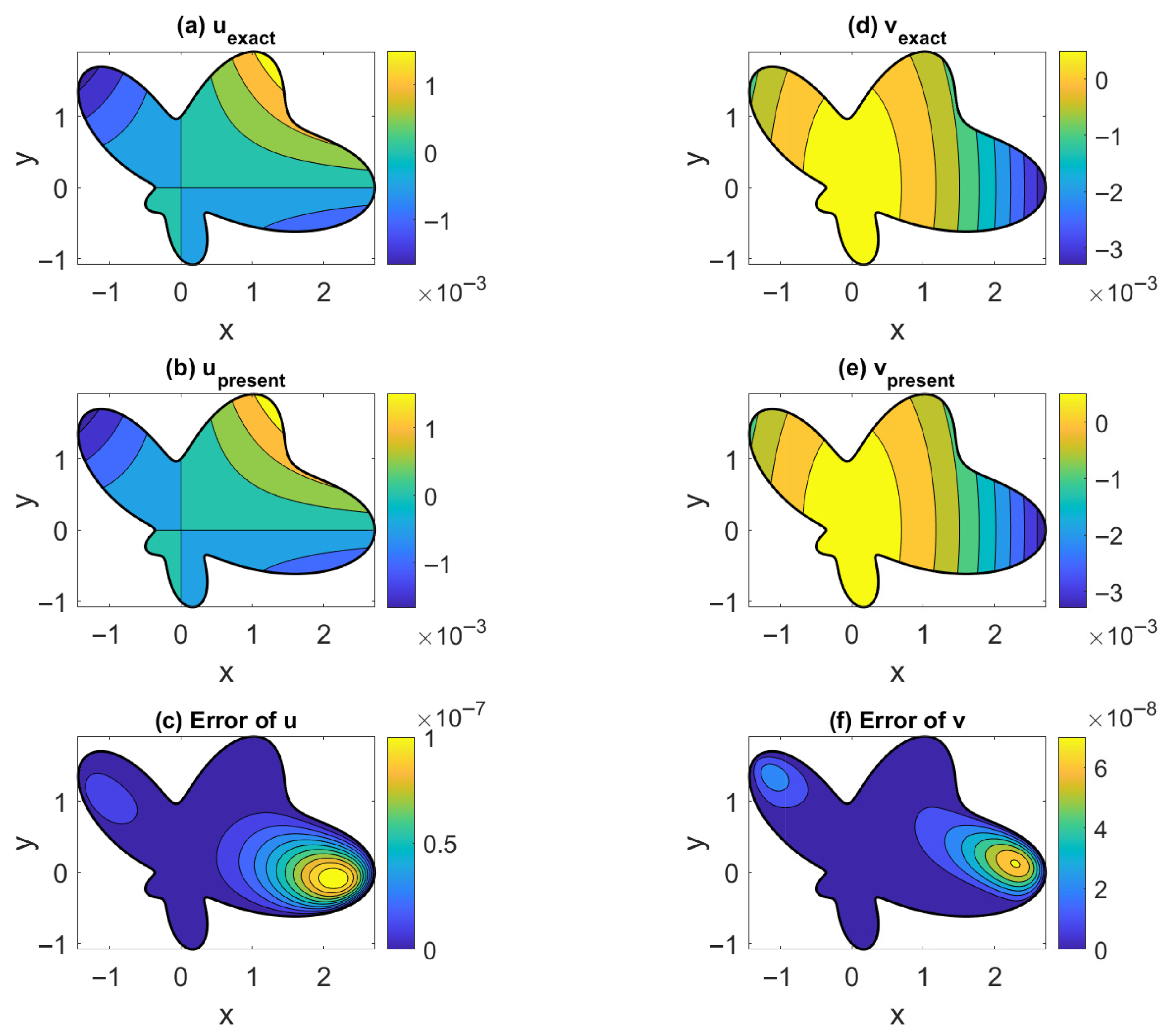
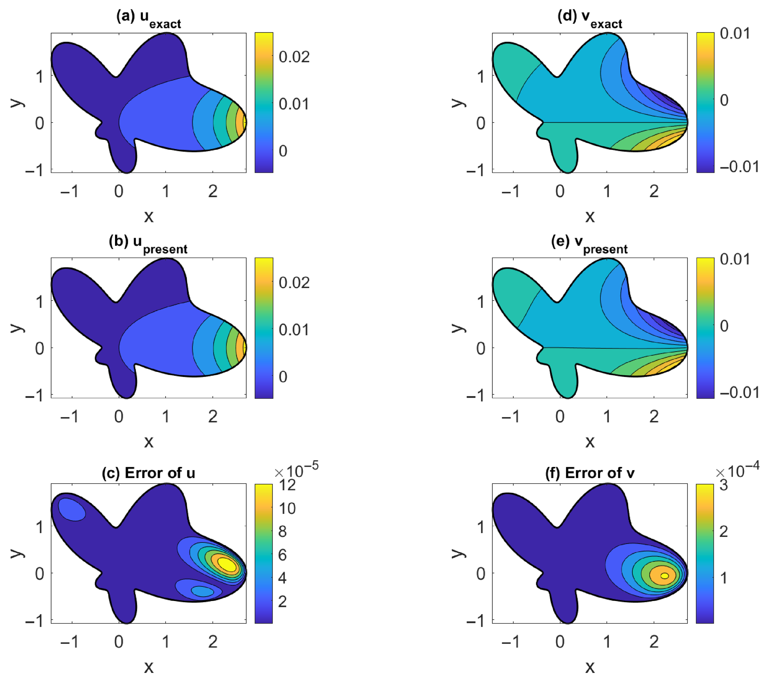
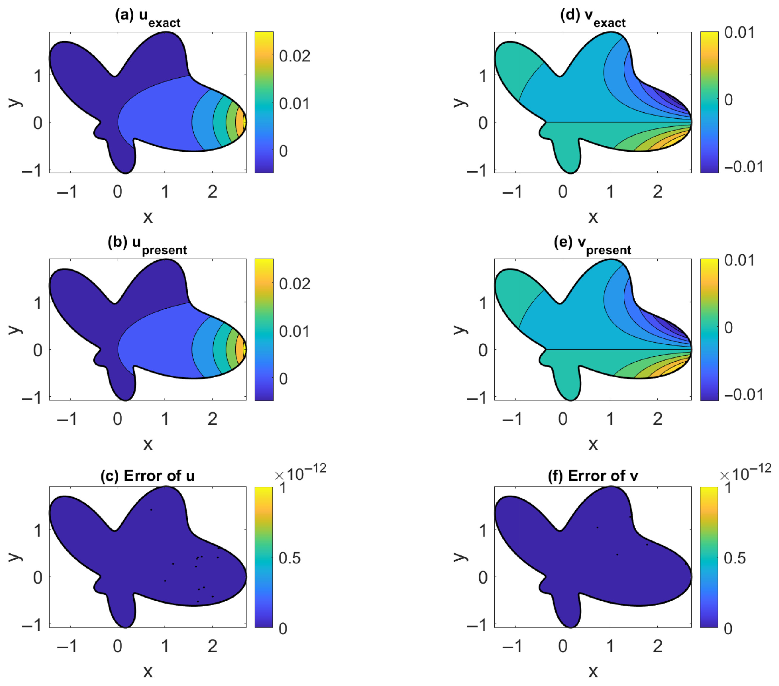
We derived the third-order MFS for effectively simulating the solutions of the 2D and 3D Navier equations. For the 2D problem, we express the solutions in terms of two harmonic functions in Theorems 1 and 2. For an incompressible material, a general solution was derived in Corollary 1 by using the anti-Cauchy–Riemann equations, whose numerical accuracy is very good, as shown by numerical examples.

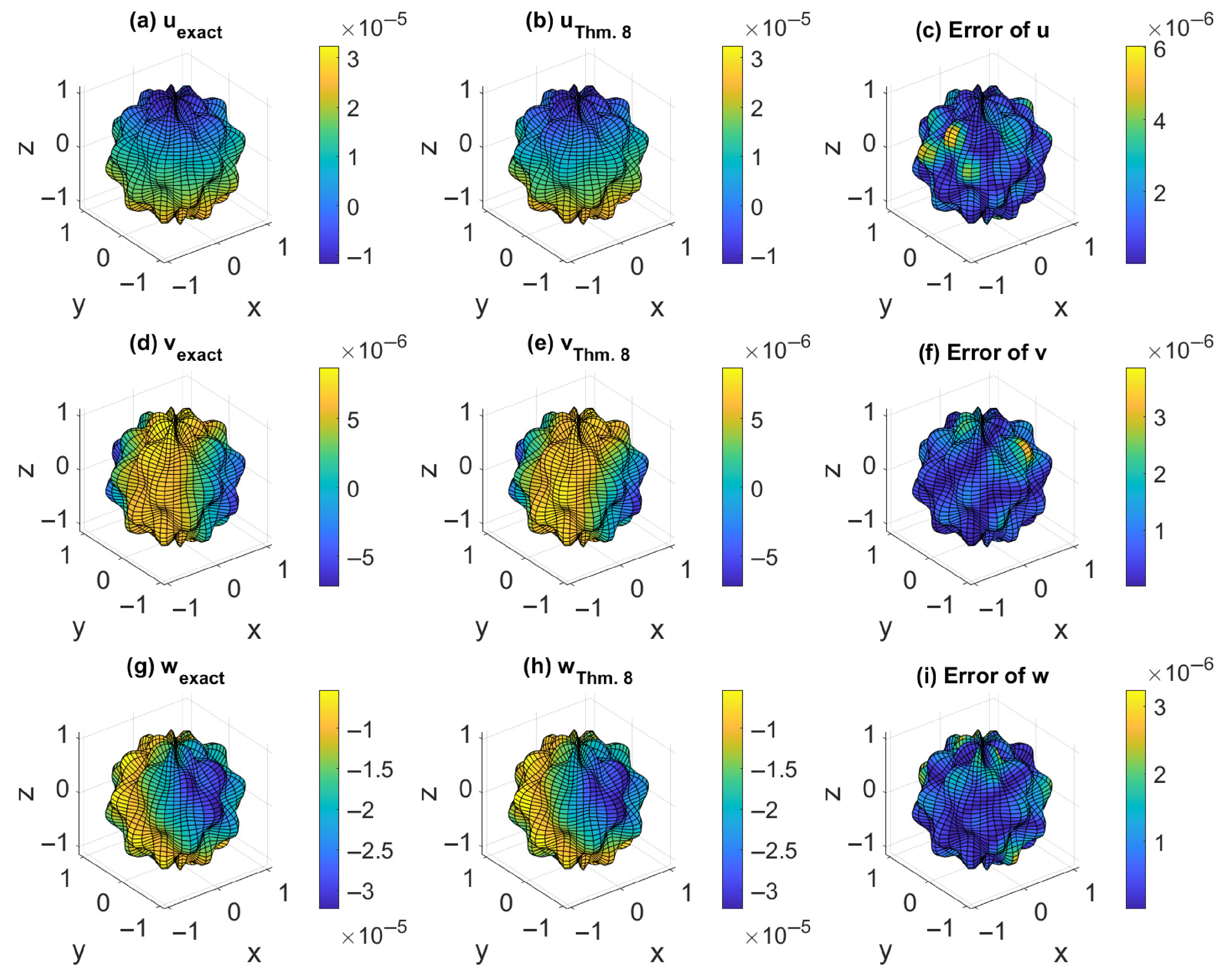
For the 3D problem, the new solutions consist of one 3D harmonic function and three 2D in-plane harmonic functions, being more efficient than the four 3D harmonic functions used in the Papkovich–Neuber solution. Three new general solutions in terms of a concentrated point force in Theorems 7–9 were derived. It is critical that only a biharmonic function and a harmonic function were needed in Theorem 7. The proof of the completeness of the solution in Theorem 7 was provided. A rather general solution was presented in Theorem 8, with a very simple form involving a harmonic vector and a concentrated point force. Theorem 8 is crucial to reducing the complete general solution in terms of three harmonic functions in the Cartesian coordinates. One theoretical achievement of this paper is that we have provided a new, simpler approach of the Slobodianskii general solution. The Slobodianskii solution is more complex than the one in Theorem 8. By using the projective solutions technique, we proved that three analytic functions can be used in the solutions in Theorem 12. Then, by merging the reduced fundamental solutions into the Papkovic–Neuber method, a powerful numerical method of the MFS type was developed.

The main novel contributions of the present paper are summarized as follows.

• Several new general solutions to the Navier equation in both 2D and 3D linear elasticity were derived, with claimed completeness, efficiency, and mathematical compactness.
• The theoretical contributions are substantial, with a minimal number of three harmonic functions to represent the complete general solution for the 3D Navier equation.
• A new, simpler approach of the Slobodianskii general solution was provided.
• How to express the new general solutions in terms of monogenic potentials and derive the generalized Kolosov–Muskhelishvili formulas would be an interesting issue.
• The extension from the MFS-type bases to the Trefftz-type bases using the novel solutions can be carried out to improve the ill-posedness of the MFS, which needs a lot of further study.
• In the future, these new general solutions will be investigated to reveal their advantages in the practical solutions of the engineering problems.