Nonoscillatory Solutions for m-th-Order Nonlinear Neutral Differential Equations with General Delays: Fixed-Point Approach and Application

Abstract

This paper investigates the existence and uniqueness of bounded nonoscillatory solutions for two classes of m-th-order nonlinear neutral differential equations that incorporate both discrete and distributed delays. By applying Banach’s fixed-point theorem, we establish sufficient conditions under which such solutions exist. The results extend and generalize previous works by relaxing assumptions on the nonlinear terms and accommodating a wider range of feedback structures, including positive, negative, bounded, and unbounded cases. The mathematical framework is unified and applicable to a broad class of problems, providing a comprehensive treatment of neutral equations beyond the first or second order. To demonstrate the practical relevance of the theoretical findings, we analyze a delayed temperature control system as an application and provide numerical simulations to illustrate nonoscillatory behavior. This paper concludes with a discussion of analytical challenges, limitations of the numerical scope, and possible future directions involving stochastic effects and more complex delay structures.

1. Introduction

Differential equations involving delayed arguments appear widely in models across the natural sciences and engineering. These equations are essential in areas such as optimal control [1], population dynamics [2], nuclear reactor theory [3], and signal transmission systems [4]. Among them, neutral differential equations constitute a significant subclass in which the derivative of the unknown function depends not only on its past values but also on delayed derivatives. This feature introduces analytical complexities beyond those in standard delay differential equations, such as difficulties in establishing compactness and ensuring well-posedness. Neutral differential equations naturally arise in various real-world contexts, including systems with memory, viscoelastic materials, and electrical networks with feedback loops.

Studying the nonoscillatory behavior of such equations is of great importance, as it relates closely to the stability and predictability of the modeled phenomena [5,6,7,8,9,10,11,12,13,14,15,16,17,18,19,20]. While oscillation theory has seen significant developments, much less attention has been given to conditions ensuring nonoscillatory solutions—especially for higher-order and nonlinear neutral equations involving distributed delays [21,22,23,24,25,26].

The purpose of this paper is to investigate the m-th-order nonlinear neutral differential equations of the forms

$$\begin{array}{cc}\hfill & {\left(\kappa \left(t\right){\left[y\left(t\right)-r\left(t\right)y\left(t-\varsigma \right)\right]}^{\left(m-1\right)}\right)}^{\prime }\hfill \\ \hfill & ={\left(-1\right)}^{m+1}\left[{\int }_{a_1}^{b_1}{g}_1\left(t,y\left({\eta }_1\left(t,\vartheta \right)\right)\right)\mathrm{d}\vartheta -{\int }_{a_2}^{b_2}{g}_2\left(t,y\left({\eta }_2\left(t,\vartheta \right)\right)\right)\mathrm{d}\vartheta -h\left(t\right)\right]\hfill \end{array}$$

(1)

and

$$\begin{array}{cc}\hfill & {\left(\kappa \left(t\right){\left[y\left(t\right)-{\int }_a^{b}R\left(t,\vartheta \right)y\left(t-\vartheta \right)\mathrm{d}\vartheta \right]}^{\left(m-1\right)}\right)}^{\prime }\hfill \\ \hfill & ={\left(-1\right)}^{m+1}\left[{\int }_{a_1}^{b_1}{g}_1\left(t,y\left({\eta }_1\left(t,\vartheta \right)\right)\right)\mathrm{d}\vartheta -{\int }_{a_2}^{b_2}{g}_2\left(t,y\left({\eta }_2\left(t,\vartheta \right)\right)\right)\mathrm{d}\vartheta -h\left(t\right)\right],\hfill \end{array}$$

(2)

where $m\ge 2$ is an integer, $h,r\in C\left(\left[t_0,\infty \right),\mathbb{R}\right)$, $\varsigma >0$, $\kappa \in C\left(\left[t_0,\infty \right),\left(0,\infty \right)\right)$, $R\in C\left(\left[t_0,\infty \right)\times \left[a,b\right],\mathbb{R}\right)$ for $0<a<b$, and ${\eta }_j\in C\left(\left[t_0,\infty \right)\times \left[a_j,b_j\right],\mathbb{R}\right)$ with ${\lim }_{t\to \infty }{\eta }_j\left(t,\vartheta \right)=\infty$ for $\vartheta \in \left[a_j,b_j\right]$, $a_j\ge 0$, $j=1,2$.

In our research, we suppose that the functions $g_j\left(t,y\right)\in C\left(\left[t_0,\infty \right)\times \mathbb{R},\mathbb{R}\right)$ are nondecreasing in y, where $y{g}_j\left(t,y\right)>0$ for $y\ne 0$ and $j=1,2$, and satisfy

$$\left|g_j\left(t,y\right)-g_j\left(t,x\right)\right|\le {\phi }_j\left(t\right)\left|y-x\right|,\mathrm{for}t\in \left[t_0,\infty \right)\mathrm{and}y,x\in \left[c,d\right],$$

(3)

where ${\phi }_j\in C\left(\left[t_0,\infty \right),\left(0,\infty \right)\right),j=1,2$, and $\left[c,d\right]$ ($0<c<d$ or $c<d<0$) is any closed interval. In addition, it is assumed that

$${\int }_{t_0}^{\infty }{\int }_{t_0}^{\xi }{\displaystyle \frac{{\xi }^{m-2}}{\kappa \left(\xi \right)}}{\phi }_j\left(v\right)\mathrm{d}v\mathrm{d}\xi <\infty ,j=1,2,$$

(4)

$${\int }_{t_0}^{\infty }{\int }_{t_0}^{\xi }{\displaystyle \frac{{\xi }^{m-2}}{\kappa \left(\xi \right)}}\left|g_j\left(v,z\right)\right|\mathrm{d}v\mathrm{d}\xi <\infty ,\mathrm{for}\mathrm{some}z\ne 0,j=1,2,$$

(5)

and

$${\int }_{t_0}^{\infty }{\int }_{t_0}^{\xi }{\displaystyle \frac{{\xi }^{m-2}}{\kappa \left(\xi \right)}}\left|h\left(v\right)\right|\mathrm{d}v\mathrm{d}\xi <\infty ,$$

(6)

hold true.

To ensure the uniqueness of the solutions established in this study, we impose a Lipschitz-type condition on the nonlinear functions $g_j\left(t,y\right)$, as specified in condition (3). This assumption plays a crucial role in guaranteeing that the associated integral operator defined in the proof of each theorem is a contraction. As such, Banach’s fixed-point theorem becomes applicable and ensures not only the existence but also the uniqueness of the nonoscillatory solution. It is important to note that relaxing the Lipschitz condition to mere continuity would preclude the use of this theorem and require alternative fixed-point tools that do not guarantee uniqueness. Therefore, the current framework carefully balances generality in nonlinearities with mathematical rigor to secure both the existence and uniqueness of the solutions.

In 2016, Candan [13] investigated nonoscillatory solutions for the following neutral differential equations with higher orders of the form

$${\left(\kappa \left(t\right){\left[{\left[y\left(t\right)-{\int }_a^{b}R\left(t,\vartheta \right)y\left(t-\vartheta \right)\mathrm{d}\vartheta \right]}^{\left(m-1\right)}\right]}^{\gamma }\right)}^{\prime }+{\left(-1\right)}^m{\int }_c^{\mathrm{d}}Q\left(t,\vartheta \right)G\left(y\left(t-\vartheta \right)\right)\mathrm{d}\vartheta =0.$$

(7)

In 2019, Şenel et al. [14] studied nonoscillatory solutions for Equations (1) and (2) in the case when $m=1$. In 2023, Cina et al. [15] investigated the existence of nonoscillatory solutions of the following nonlinear neutral differential equation of the m -th order and the following forcing term:

$${\left(\kappa \left(t\right){\left[y\left(t\right)-r\left(t\right)y\left(t-\varsigma \right)\right]}^{\left(m-1\right)}\right)}^{\prime }+{\left(-1\right)}^m\left[g_1\left(t,y\left({\eta }_1\left(t\right)\right)\right)-g_2\left(t,y\left({\eta }_2\left(t\right)\right)\right)-h\left(t\right)\right]=0.$$

(8)

Building upon foundational works such as those by [13,14,15], this paper establishes new sufficient conditions for the existence and uniqueness of nonoscillatory solutions to m-th-order nonlinear neutral differential equations. By employing Banach’s fixed-point theorem, we extend previous results to a more generalized and unified theoretical framework that accommodates both discrete and distributed delays under relaxed assumptions. Unlike earlier studies—particularly [15], which focused primarily on lower-order equations with limited types of delay arguments—our work systematically addresses a wider range of neutral feedback scenarios, including positive, negative, bounded, and unbounded cases. This broadens the analytical scope and captures a richer variety of dynamic behaviors. The practical relevance of the theoretical results is demonstrated through a representative application to delayed control systems, with numerical simulations validating the predicted nonoscillatory behavior in the context of temperature regulation.

Let

$$T_0=\min \left\{t^{\ast }-\varsigma ,\underset{\begin{array}{c}t\ge t^{\ast }\\ j=1,2\end{array}}{\inf }\left(\underset{\vartheta \in \left[a_j,b_j\right]}{\min }{\eta }_j\left(t,\vartheta \right)\right)\right\},$$

for $t^{\ast }\ge t_0$. Using the solution of Equation (1), the function $y\in C\left(\left[T_0,\infty \right),\mathbb{R}\right)$ means that $\kappa \left(t\right){\left[y\left(t\right)-r\left(t\right)y\left(t-\varsigma \right)\right]}^{m-1}$ is continuously differentiable on $\left[t^{\ast },\infty \right)$ and $y\left(t\right)-r\left(t\right)y\left(t-\varsigma \right)$ is $m-1$ times continuously differentiable on $\left[t^{\ast },\infty \right)$, where Equation (1) is satisfied for $t\ge t^{\ast }$.

Let

$$T_1=\min \left\{t^{\ast }-b,\underset{\begin{array}{c}t\ge t^{\ast }\\ j=1,2\end{array}}{\inf }\left(\underset{\vartheta \in \left[a_j,b_j\right]}{\min }{\eta }_j\left(t,\vartheta \right)\right)\right\},$$

for $t^{\ast }\ge t_0$. Using the solution of Equation (2), the function $y\in C\left(\left[T_1,\infty \right),\mathbb{R}\right)$ means that $\kappa \left(t\right){\left[y\left(t\right)-{\int }_a^{b}R\left(t,\vartheta \right)y\left(t-\vartheta \right)\mathrm{d}\vartheta \right]}^{\left(m-1\right)}$ is continuously differentiable on $\left[t^{\ast },\infty \right)$ and $y\left(t\right)-{\int }_a^{b}R\left(t,\vartheta \right)y\left(t-\vartheta \right)\mathrm{d}\vartheta$ is $m-1$ times continuously differentiable on $\left[t^{\ast },\infty \right)$, where Equation (2) is satisfied for $t\ge t^{\ast }$.

The structure of this paper is as follows: Section 2 introduces the main results and provides detailed proofs using fixed-point theory. Section 3 includes numerical simulations to illustrate the nonoscillatory behavior of solutions in control systems. Finally, Section 4 presents conclusions and directions for future research.

2. Main Results

In this section, we establish the theoretical framework necessary for analyzing the existence of nonoscillatory solutions in higher-order nonlinear neutral differential equations. The section is structured as follows: In Section 2.1, we provide the main theorems of Equation (1), and in Section 2.2, we provide the main theorems of Equation (2).

Let Y be the space of all continuous and bounded functions on $\left[t_0,\infty \right)$ equipped with the norm

$$∥y∥=\underset{t\ge t_0}{\sup }\left|y\left(t\right)\right|<\infty .$$

Definition 1.

We define a solution of the differential Equations (1) or (2) as oscillatory if it has arbitrarily large zeros. Otherwise, the solution of these equations is nonoscillatory.

2.1. Nonoscillatory Characteristics and Boundedness of Equation (1)

Theorem 1.

Suppose that (3)–(6) hold and $0\le r\left(t\right)\le \rho <1$. Then, Equation (1) has a bounded nonoscillatory solution.

Proof. 

Assume that condition (5) holds such that $W_2:=z>0$ and, in a similar manner, holds for $z<0$. Let

$$B_1=\left\{y\in Y:W_1\le y\left(t\right)\le W_2,t\ge t_0\right\},$$

such that $W_1$ and $W_2$ are positive constants that satisfy

$$W_1<(1-\rho )W_2.$$

Clearly, $B_1$ is a bounded, closed, and convex subset of Y. According to (4)–(6), there exists a number $t^{\ast }$ that is sufficiently large enough to satisfy $t^{\ast }>t_0$ such that $t-\varsigma \ge t_0$, ${\eta }_j\left(t,\vartheta \right)\ge t_0,\vartheta \in \left[a_j,b_j\right],j=1,2$, for $t\ge t^{\ast }$ and

$$\rho +{\displaystyle \frac{1}{\left(m-2\right)!}}{\int }_{t^{\ast }}^{\infty }{\int }_{t^{\ast }}^{\xi }{\displaystyle \frac{{\left(\xi -t\right)}^{m-2}}{\kappa \left(\xi \right)}}\sum _{j=1}^2\left(b_j-a_j\right){\phi }_j\left(v\right)\mathrm{d}v\mathrm{d}\xi \le {\delta }_1<1,$$

(9)

where ${\delta }_1$ is a constant, and

$${\displaystyle \frac{1}{\left(m-2\right)!}}{\int }_{t^{\ast }}^{\infty }{\int }_{t^{\ast }}^{\xi }{\displaystyle \frac{{\left(\xi -t\right)}^{m-2}}{\kappa \left(\xi \right)}}\left[\left(b_1-a_1\right)g_1\left(v,z\right)+\left|h\left(v\right)\right|\right]\mathrm{d}v\mathrm{d}\xi \le \left(1-\rho \right)W_2-\alpha ,$$

(10)

$${\displaystyle \frac{1}{\left(m-2\right)!}}{\int }_{t^{\ast }}^{\infty }{\int }_{t^{\ast }}^{\xi }{\displaystyle \frac{{\left(\xi -t\right)}^{m-2}}{\kappa \left(\xi \right)}}\left[\left(b_2-a_2\right)g_2\left(v,z\right)+\left|h\left(v\right)\right|\right]\mathrm{d}v\mathrm{d}\xi \le \alpha -W_1,$$

(11)

where $\alpha \in \left(W_1,\left(1-\rho \right)W_2\right)$.

The operator $S_1$ is defined on $B_1$ by

$$\left(S_{1}y\right)\left(t\right)=\left\{\begin{array}{c}\alpha +r\left(t\right)y\left(t-\varsigma \right)+{\displaystyle \frac{1}{\left(m-2\right)!}}{\int }_t^{\infty }{\displaystyle \frac{{\left(\xi -t\right)}^{m-2}}{\kappa \left(\xi \right)}}\hfill \\ \times {\int }_{t^{\ast }}^{\xi }\left[{\int }_{a_1}^{b_1}{g}_1\left(v,y\left({\eta }_1\left(v,\vartheta \right)\right)\right)\mathrm{d}\vartheta -{\int }_{a_2}^{b_2}{g}_2\left(v,y\left({\eta }_2\left(v,\vartheta \right)\right)\right)\mathrm{d}\vartheta -h\left(v\right)\right]\mathrm{d}v\mathrm{d}\xi ,t\ge t^{\ast }\hfill \\ \left(S_{1}y\right)\left(t^{\ast }\right),t_0\le t\le t^{\ast }.\hfill \end{array}\right.$$

It can be readily observed that $S_{1}y$ is a continuous operator. We will prove that $S_1{B}_1\subset B_1$. Indeed, for every $y\in B_1$ and $t\ge t^{\ast }$, due to (10), we have

$$\begin{array}{ccc}\hfill \left(S_{1}y\right)\left(t\right)& =& \alpha +r\left(t\right)y\left(t-\varsigma \right)+{\displaystyle \frac{1}{\left(m-2\right)!}}{\int }_t^{\infty }{\displaystyle \frac{{\left(\xi -t\right)}^{m-2}}{\kappa \left(\xi \right)}}\hfill \\ & & \times {\int }_{t^{\ast }}^{\xi }\left[{\int }_{a_1}^{b_1}{g}_1\left(v,y\left({\eta }_1\left(v,\vartheta \right)\right)\right)\mathrm{d}\vartheta -{\int }_{a_2}^{b_2}{g}_2\left(v,y\left({\eta }_2\left(v,\vartheta \right)\right)\right)\mathrm{d}\vartheta -h\left(v\right)\right]\mathrm{d}v\mathrm{d}\xi \hfill \\ & \le & \alpha +\rho W_2+{\displaystyle \frac{1}{\left(m-2\right)!}}{\int }_{t^{\ast }}^{\infty }{\int }_{t^{\ast }}^{\xi }{\displaystyle \frac{{\left(\xi -t\right)}^{m-2}}{\kappa \left(\xi \right)}}\left[\left(b_1-a_1\right)g_1\left(v,z\right)+\left|h\left(v\right)\right|\right]\mathrm{d}v\mathrm{d}\xi \hfill \\ & \le & \alpha +\rho W_2+\left(1-\rho \right)W_2-\alpha \hfill \\ & =& W_2,\hfill \end{array}$$

and taking (11) into account, we have

$$\begin{array}{ccc}\hfill \left(S_{1}y\right)\left(t\right)& =& \alpha +r\left(t\right)y\left(t-\varsigma \right)+{\displaystyle \frac{1}{\left(m-2\right)!}}{\int }_t^{\infty }{\displaystyle \frac{{\left(\xi -t\right)}^{m-2}}{\kappa \left(\xi \right)}}\hfill \\ & & \times {\int }_{t^{\ast }}^{\xi }\left[{\int }_{a_1}^{b_1}{g}_1\left(v,y\left({\eta }_1\left(v,\vartheta \right)\right)\right)\mathrm{d}\vartheta -{\int }_{a_2}^{b_2}{g}_2\left(v,y\left({\eta }_2\left(v,\vartheta \right)\right)\right)\mathrm{d}\vartheta -h\left(v\right)\right]\mathrm{d}v\mathrm{d}\xi \hfill \\ & \ge & \alpha -{\displaystyle \frac{1}{\left(m-2\right)!}}{\int }_{t^{\ast }}^{\infty }{\int }_{t^{\ast }}^{\xi }{\displaystyle \frac{{\left(\xi -t\right)}^{m-2}}{\kappa \left(\xi \right)}}\left[\left(b_2-a_2\right)g_2\left(v,z\right)+\left|h\left(v\right)\right|\right]\mathrm{d}v\mathrm{d}\xi \hfill \\ & \ge & \alpha -\alpha +W_1\hfill \\ & =& W_1.\hfill \end{array}$$

Hence, we conclude that $S_1{B}_1\subset B_1$.

Next, we demonstrate that $S_1$ is a contraction operator on $B_1$. Indeed, for $y,x\in B_1$ and $t\ge t^{\ast }$, using (3) and (9), we obtain

$$\begin{array}{ccc}\hfill \left|\left(S_{1}y\right)\left(t\right)-\left(S_{1}x\right)\left(t\right)\right|& \le & \rho \left|y\left(t-\varsigma \right)-x\left(t-\varsigma \right)\right|+{\displaystyle \frac{1}{\left(m-2\right)!}}{\int }_t^{\infty }{\displaystyle \frac{{\left(\xi -t\right)}^{m-2}}{\kappa \left(\xi \right)}}\hfill \\ & & \times {\int }_{t^{\ast }}^{\xi }\sum _{j=1}^2{\int }_{a_j}^{b_j}\left|g_j\left(v,y\left({\eta }_j\left(v,\vartheta \right)\right)\right)-g_j\left(v,x\left({\eta }_j\left(v,\vartheta \right)\right)\right)\right|\mathrm{d}\vartheta \mathrm{d}v\mathrm{d}\xi \hfill \\ & \le & \rho \left|y\left(t-\varsigma \right)-x\left(t-\varsigma \right)\right|+{\displaystyle \frac{1}{\left(m-2\right)!}}{\int }_t^{\infty }{\displaystyle \frac{{\left(\xi -t\right)}^{m-2}}{\kappa \left(\xi \right)}}\hfill \\ & & \times {\int }_{t^{\ast }}^{\xi }\sum _{j=1}^2{\int }_{a_j}^{b_j}{\phi }_j\left(v\right)\left|y\left({\eta }_j\left(v,\vartheta \right)\right)-x\left({\eta }_j\left(v,\vartheta \right)\right)\right|\mathrm{d}\vartheta \mathrm{d}v\mathrm{d}\xi \hfill \\ & \le & ∥y-x∥\left[\rho +{\displaystyle \frac{1}{\left(m-2\right)!}}{\int }_{t^{\ast }}^{\infty }{\int }_{t^{\ast }}^{\xi }{\displaystyle \frac{{\left(\xi -t\right)}^{m-2}}{\kappa \left(\xi \right)}}\sum _{j=1}^2\left(b_j-a_j\right){\phi }_j\left(v\right)\mathrm{d}v\mathrm{d}\xi \right]\hfill \\ & \le & {\delta }_1∥y-x∥,\hfill \end{array}$$

which implies that

$$∥S_{1}y-S_{1}x∥\le {\delta }_1∥y-x∥.$$

Since ${\delta }_1<1$, then $S_1$ is a contraction mapping on $B_1$. As a consequence, $S_1$ has the unique fixed point $y\in B_1$, which is obviously a positive solution of (1). □

Theorem 2.

Assume that (3)–(6) hold and $1<{\rho }_1\le r\left(t\right)\le {\rho }_2<\infty$. Then, Equation (1) has a bounded nonoscillatory solution.

Proof. 

Assume condition (5) holds such that $W_4:=z>0$ and, in a similar manner, holds for $z<0$. Let

$$B_2=\left\{y\in Y:W_3\le y\left(t\right)\le W_4,t\ge t_0\right\},$$

such that $W_3$ and $W_4$ are positive constants that satisfy

$${\rho }_2{W}_3<\left({\rho }_1-1\right)W_4.$$

It is obvious that $B_2$ is a bounded, closed, and convex subset of Y. According to (4)–(6), there exists a number $t^{\ast }$ that is sufficiently large enough to satisfy $t^{\ast }>t_0$ such that ${\eta }_j\left(t+\varsigma ,\vartheta \right)\ge t_0,\vartheta \in \left[a_j,b_j\right],j=1,2$, for $t\ge t^{\ast }$ and

$${\displaystyle \frac{1}{{\rho }_1}}\left[1+{\displaystyle \frac{1}{\left(m-2\right)!}}{\int }_{t^{\ast }}^{\infty }{\int }_{t^{\ast }}^{\xi }{\displaystyle \frac{{\left(\xi -t\right)}^{m-2}}{\kappa \left(\xi \right)}}\sum _{j=1}^2\left(b_j-a_j\right){\phi }_j\left(v\right)\mathrm{d}v\mathrm{d}\xi \right]\le {\delta }_2<1,$$

(12)

where ${\delta }_2$ is a constant, and

$${\displaystyle \frac{1}{\left(m-2\right)!}}{\int }_{t^{\ast }}^{\infty }{\int }_{t^{\ast }}^{\xi }{\displaystyle \frac{{\left(\xi -t\right)}^{m-2}}{\kappa \left(\xi \right)}}\left[\left(b_1-a_1\right)g_1\left(v,z\right)+\left|h\left(v\right)\right|\right]\mathrm{d}v\mathrm{d}\xi \le \alpha -{\rho }_2{W}_3,$$

(13)

$${\displaystyle \frac{1}{\left(m-2\right)!}}{\int }_{t^{\ast }}^{\infty }{\int }_{t^{\ast }}^{\xi }{\displaystyle \frac{{\left(\xi -t\right)}^{m-2}}{\kappa \left(\xi \right)}}\left[\left(b_2-a_2\right)g_2\left(v,z\right)+\left|h\left(v\right)\right|\right]\mathrm{d}v\mathrm{d}\xi \le \left({\rho }_1-1\right)W_4-\alpha ,$$

(14)

where $\alpha \in \left({\rho }_2{W}_3,\left({\rho }_1-1\right)W_4\right)$.

The operator $S_2$ is defined on $B_2$ by

$$\left(S_{2}y\right)\left(t\right)=\left\{\begin{array}{c}{\displaystyle \frac{1}{r\left(t+\varsigma \right)}}\left[\alpha +y\left(t+\varsigma \right)+{\displaystyle \frac{1}{\left(m-2\right)!}}{\int }_{t+\varsigma }^{\infty }{\displaystyle \frac{{\left(\xi -\varsigma -t\right)}^{m-2}}{\kappa \left(\xi \right)}}\right.\hfill \\ \left.\times {\int }_{t^{\ast }+\varsigma }^{\xi }\left[{\int }_{a_1}^{b_1}{g}_1\left(v,y\left({\eta }_1\left(v,\vartheta \right)\right)\right)\mathrm{d}\vartheta -{\int }_{a_2}^{b_2}{g}_2\left(v,y\left({\eta }_2\left(v,\vartheta \right)\right)\right)\mathrm{d}\vartheta -h\left(v\right)\right]\mathrm{d}v\mathrm{d}\xi \right],t\ge t^{\ast }\hfill \\ \left(S_{2}y\right)\left(t^{\ast }\right),t_0\le t\le t^{\ast }.\hfill \end{array}\right.$$

It can be readily observed that $S_{2}y$ is a continuous operator. We will prove that $S_2{B}_2\subset B_2$. Indeed, for every $y\in B_2$ and $t\ge t^{\ast }$, due to (14), we have

$$\begin{array}{ccc}\hfill \left(S_{2}y\right)\left(t\right)& =& {\displaystyle \frac{1}{r\left(t+\varsigma \right)}}\left[\alpha +y\left(t+\varsigma \right)+{\displaystyle \frac{1}{\left(m-2\right)!}}{\int }_{t+\varsigma }^{\infty }{\displaystyle \frac{{\left(\xi -\varsigma -t\right)}^{m-2}}{\kappa \left(\xi \right)}}\right.\hfill \\ & & \left.\times {\int }_{t^{\ast }+\varsigma }^{\xi }\left[{\int }_{a_1}^{b_1}{g}_1\left(v,y\left({\eta }_1\left(v,\vartheta \right)\right)\right)\mathrm{d}\vartheta -{\int }_{a_2}^{b_2}{g}_2\left(v,y\left({\eta }_2\left(v,\vartheta \right)\right)\right)\mathrm{d}\vartheta -h\left(v\right)\right]\mathrm{d}v\mathrm{d}\xi \right]\hfill \\ & \le & {\displaystyle \frac{1}{{\rho }_1}}\left[\alpha +W_4+{\displaystyle \frac{1}{\left(m-2\right)!}}{\int }_{t^{\ast }}^{\infty }{\int }_{t^{\ast }}^{\xi }{\displaystyle \frac{{\left(\xi -t\right)}^{m-2}}{\kappa \left(\xi \right)}}\left[\left(b_2-a_2\right)g_2\left(v,z\right)+\left|h\left(v\right)\right|\right]\mathrm{d}v\mathrm{d}\xi \right]\hfill \\ & \le & {\displaystyle \frac{1}{{\rho }_1}}\left[\alpha +W_4+\left({\rho }_1-1\right)W_4-\alpha \right]\hfill \\ & =& W_4,\hfill \end{array}$$

and taking (13) into account, we have

$$\begin{array}{ccc}\hfill \left(S_{2}y\right)\left(t\right)& =& {\displaystyle \frac{1}{r\left(t+\varsigma \right)}}\left[\alpha +y\left(t+\varsigma \right)+{\displaystyle \frac{1}{\left(m-2\right)!}}{\int }_{t+\varsigma }^{\infty }{\displaystyle \frac{{\left(\xi -\varsigma -t\right)}^{m-2}}{\kappa \left(\xi \right)}}\right.\hfill \\ & & \left.\times {\int }_{t^{\ast }+\varsigma }^{\xi }\left[{\int }_{a_1}^{b_1}{g}_1\left(v,y\left({\eta }_1\left(v,\vartheta \right)\right)\right)\mathrm{d}\vartheta -{\int }_{a_2}^{b_2}{g}_2\left(v,y\left({\eta }_2\left(v,\vartheta \right)\right)\right)\mathrm{d}\vartheta -h\left(v\right)\right]\mathrm{d}v\mathrm{d}\xi \right]\hfill \\ & \ge & {\displaystyle \frac{1}{{\rho }_2}}\left[\alpha -{\displaystyle \frac{1}{\left(m-2\right)!}}{\int }_{t^{\ast }}^{\infty }{\int }_{t^{\ast }}^{\xi }{\displaystyle \frac{{\left(\xi -t\right)}^{m-2}}{\kappa \left(\xi \right)}}\left[\left(b_1-a_1\right)g_1\left(v,z\right)+\left|h\left(v\right)\right|\right]\mathrm{d}v\mathrm{d}\xi \right]\hfill \\ & \ge & {\displaystyle \frac{1}{{\rho }_2}}\left[\alpha -\alpha +{\rho }_2{W}_3\right]\hfill \\ & =& W_3.\hfill \end{array}$$

Hence, we conclude that $S_2{B}_2\subset B_2$.

Next, we prove that $S_2$ is a contraction operator on $B_2$. Indeed, for $y,x\in B_2$ and $t\ge t^{\ast }$, using (3) and (12), we obtain

$$\begin{array}{ccc}\hfill \left|\left(S_{2}y\right)\left(t\right)-\left(S_{2}x\right)\left(t\right)\right|& \le & {\displaystyle \frac{1}{{\rho }_1}}\left|y\left(t+\varsigma \right)-x\left(t+\varsigma \right)\right|+{\displaystyle \frac{1}{{\rho }_1\left(m-2\right)!}}{\int }_t^{\infty }{\displaystyle \frac{{\left(\xi -\varsigma -t\right)}^{m-2}}{\kappa \left(\xi \right)}}\hfill \\ & & \times {\int }_{t^{\ast }}^{\xi }\sum _{j=1}^2{\int }_{a_j}^{b_j}\left|g_j\left(v,y\left({\eta }_j\left(v,\vartheta \right)\right)\right)-g_j\left(v,x\left({\eta }_j\left(v,\vartheta \right)\right)\right)\right|\mathrm{d}\vartheta \mathrm{d}v\mathrm{d}\xi \hfill \\ & \le & {\displaystyle \frac{1}{{\rho }_1}}\left|y\left(t-\varsigma \right)-x\left(t-\varsigma \right)\right|+{\displaystyle \frac{1}{{\rho }_1\left(m-2\right)!}}{\int }_t^{\infty }{\displaystyle \frac{{\left(\xi -t\right)}^{m-2}}{\kappa \left(\xi \right)}}\hfill \\ & & \times {\int }_{t^{\ast }}^{\xi }\sum _{j=1}^2{\int }_{a_j}^{b_j}{\phi }_j\left(v\right)\left|y\left({\eta }_j\left(v,\vartheta \right)\right)-x\left({\eta }_j\left(v,\vartheta \right)\right)\right|\mathrm{d}\vartheta \mathrm{d}v\mathrm{d}\xi \hfill \\ & \le & ∥y-x∥{\displaystyle \frac{1}{{\rho }_1}}\left[1+{\displaystyle \frac{1}{\left(m-2\right)!}}{\int }_{t^{\ast }}^{\infty }{\int }_{t^{\ast }}^{\xi }{\displaystyle \frac{{\left(\xi -t\right)}^{m-2}}{\kappa \left(\xi \right)}}\sum _{j=1}^2\left(b_j-a_j\right){\phi }_j\left(v\right)\mathrm{d}v\mathrm{d}\xi \right]\hfill \\ & \le & {\delta }_2∥y-x∥,\hfill \end{array}$$

which implies that

$$∥S_{2}y-S_{2}x∥\le {\delta }_2∥y-x∥.$$

Since ${\delta }_2<1$, then $S_2$ is a contraction mapping on $B_2$. As a consequence, $S_2$ has the unique fixed point $y\in B_2$, which is obviously a positive solution of (1). □

Theorem 3.

Assume that (3)–(6) hold and $-1<-\rho \le r\left(t\right)\le 0$. Then, Equation (1) has a bounded nonoscillatory solution.

Proof. 

Assume that condition (5) holds such that $W_6:=z>0$ and, in a similar manner, holds for $z<0$. Let

$$B_3=\left\{y\in Y:W_5\le y\left(t\right)\le W_6,t\ge t_0\right\},$$

such that $W_5$ and $W_6$ are positive constants that satisfy

$$W_5+\rho W_6<W_6.$$

Clearly, $B_3$ is a bounded, closed, and convex subset of Y. According to (4)–(6), there exists a number $t^{\ast }$ that is sufficiently large enough to satisfy $t^{\ast }>t_0$ such that $t-\varsigma \ge t_0$, ${\eta }_j\left(t,\vartheta \right)\ge t_0,\vartheta \in \left[a_j,b_j\right],j=1,2$, for $t\ge t^{\ast }$ and

$$\rho +{\displaystyle \frac{1}{\left(m-2\right)!}}{\int }_{t^{\ast }}^{\infty }{\int }_{t^{\ast }}^{\xi }{\displaystyle \frac{{\left(\xi -t\right)}^{m-2}}{\kappa \left(\xi \right)}}\sum _{j=1}^2\left(b_j-a_j\right){\phi }_j\left(v\right)\mathrm{d}v\mathrm{d}\xi \le {\delta }_3<1,$$

(15)

where ${\delta }_3$ is a constant, and

$${\displaystyle \frac{1}{\left(m-2\right)!}}{\int }_{t^{\ast }}^{\infty }{\int }_{t^{\ast }}^{\xi }{\displaystyle \frac{{\left(\xi -t\right)}^{m-2}}{\kappa \left(\xi \right)}}\left[\left(b_1-a_1\right)g_1\left(v,z\right)+\left|h\left(v\right)\right|\right]\mathrm{d}v\mathrm{d}\xi \le W_6-\alpha ,$$

(16)

$${\displaystyle \frac{1}{\left(m-2\right)!}}{\int }_{t^{\ast }}^{\infty }{\int }_{t^{\ast }}^{\xi }{\displaystyle \frac{{\left(\xi -t\right)}^{m-2}}{\kappa \left(\xi \right)}}\left[\left(b_2-a_2\right)g_2\left(v,z\right)+\left|h\left(v\right)\right|\right]\mathrm{d}v\mathrm{d}\xi \le \alpha -W_5-\rho W_6,$$

(17)

where $\alpha \in \left(W_5+\rho W_6,W_6\right)$.

The operator $S_3$ is defined on $B_3$ by

$$\left(S_{3}y\right)\left(t\right)=\left\{\begin{array}{c}\alpha +r\left(t\right)y\left(t-\varsigma \right)+{\displaystyle \frac{1}{\left(m-2\right)!}}{\int }_t^{\infty }{\displaystyle \frac{{\left(\xi -t\right)}^{m-2}}{\kappa \left(\xi \right)}}\hfill \\ \times {\int }_{t^{\ast }}^{\xi }\left[{\int }_{a_1}^{b_1}{g}_1\left(v,y\left({\eta }_1\left(v,\vartheta \right)\right)\right)\mathrm{d}\vartheta -{\int }_{a_2}^{b_2}{g}_2\left(v,y\left({\eta }_2\left(v,\vartheta \right)\right)\right)\mathrm{d}\vartheta -h\left(v\right)\right]\mathrm{d}v\mathrm{d}\xi ,t\ge t^{\ast }\hfill \\ \left(S_{3}y\right)\left(t^{\ast }\right),t_0\le t\le t^{\ast }.\hfill \end{array}\right.$$

It can be readily observed that $S_{3}y$ is a continuous operator. We demonstrate that $S_3{B}_3\subset B_3$. Indeed, for every $y\in B_3$ and $t\ge t^{\ast }$, due to (16), we obtain

$$\begin{array}{ccc}\hfill \left(S_{3}y\right)\left(t\right)& =& \alpha +r\left(t\right)y\left(t-\varsigma \right)+{\displaystyle \frac{1}{\left(m-2\right)!}}{\int }_t^{\infty }{\displaystyle \frac{{\left(\xi -t\right)}^{m-2}}{\kappa \left(\xi \right)}}\hfill \\ & & \times {\int }_{t^{\ast }}^{\xi }\left[{\int }_{a_1}^{b_1}{g}_1\left(v,y\left({\eta }_1\left(v,\vartheta \right)\right)\right)\mathrm{d}\vartheta -{\int }_{a_2}^{b_2}{g}_2\left(v,y\left({\eta }_2\left(v,\vartheta \right)\right)\right)\mathrm{d}\vartheta -h\left(v\right)\right]\mathrm{d}v\mathrm{d}\xi \hfill \\ & \le & \alpha +{\displaystyle \frac{1}{\left(m-2\right)!}}{\int }_{t^{\ast }}^{\infty }{\int }_{t^{\ast }}^{\xi }{\displaystyle \frac{{\left(\xi -t\right)}^{m-2}}{\kappa \left(\xi \right)}}\left[\left(b_1-a_1\right)g_1\left(v,z\right)+\left|h\left(v\right)\right|\right]\mathrm{d}v\mathrm{d}\xi \hfill \\ & \le & \alpha +W_6-\alpha \hfill \\ & =& W_6,\hfill \end{array}$$

and taking (17) into account, we have

$$\begin{array}{ccc}\hfill \left(S_{3}y\right)\left(t\right)& =& \alpha +r\left(t\right)y\left(t-\varsigma \right)+{\displaystyle \frac{1}{\left(m-2\right)!}}{\int }_t^{\infty }{\displaystyle \frac{{\left(\xi -t\right)}^{m-2}}{\kappa \left(\xi \right)}}\hfill \\ & & \times {\int }_{t^{\ast }}^{\xi }\left[{\int }_{a_1}^{b_1}{g}_1\left(v,y\left({\eta }_1\left(v,\vartheta \right)\right)\right)\mathrm{d}\vartheta -{\int }_{a_2}^{b_2}{g}_2\left(v,y\left({\eta }_2\left(v,\vartheta \right)\right)\right)\mathrm{d}\vartheta -h\left(v\right)\right]\mathrm{d}v\mathrm{d}\xi \hfill \\ & \ge & \alpha -{\displaystyle \frac{1}{\left(m-2\right)!}}{\int }_{t^{\ast }}^{\infty }{\int }_{t^{\ast }}^{\xi }{\displaystyle \frac{{\left(\xi -t\right)}^{m-2}}{\kappa \left(\xi \right)}}\left[\left(b_2-a_2\right)g_2\left(v,z\right)+\left|h\left(v\right)\right|\right]\mathrm{d}v\mathrm{d}\xi \hfill \\ & \ge & \alpha -\rho W_6-\left(\alpha -W_5-\rho W_6\right)\hfill \\ & =& W_5.\hfill \end{array}$$

Hence, we conclude that $S_3{B}_3\subset B_3$.

Next, we prove that $S_3$ is a contraction operator on $B_3$. Indeed, for $y,x\in B_3$ and $t\ge t^{\ast }$, using (3) and (15), we obtain

$$\begin{array}{ccc}\hfill \left|\left(S_{3}y\right)\left(t\right)-\left(S_{3}x\right)\left(t\right)\right|& \le & \rho \left|y\left(t-\varsigma \right)-x\left(t-\varsigma \right)\right|+{\displaystyle \frac{1}{\left(m-2\right)!}}{\int }_t^{\infty }{\displaystyle \frac{{\left(\xi -t\right)}^{m-2}}{\kappa \left(\xi \right)}}\hfill \\ & & \times {\int }_{t^{\ast }}^{\xi }\sum _{j=1}^2{\int }_{a_j}^{b_j}\left|g_j\left(v,y\left({\eta }_j\left(v,\vartheta \right)\right)\right)-g_j\left(v,x\left({\eta }_j\left(v,\vartheta \right)\right)\right)\right|\mathrm{d}\vartheta \mathrm{d}v\mathrm{d}\xi \hfill \\ & \le & \rho \left|y\left(t-\varsigma \right)-x\left(t-\varsigma \right)\right|+{\displaystyle \frac{1}{\left(m-2\right)!}}{\int }_t^{\infty }{\displaystyle \frac{{\left(\xi -t\right)}^{m-2}}{\kappa \left(\xi \right)}}\hfill \\ & & \times {\int }_{t^{\ast }}^{\xi }\sum _{j=1}^2{\int }_{a_j}^{b_j}{\phi }_j\left(v\right)\left|y\left({\eta }_j\left(v,\vartheta \right)\right)-x\left({\eta }_j\left(v,\vartheta \right)\right)\right|\mathrm{d}\vartheta \mathrm{d}v\mathrm{d}\xi \hfill \\ & \le & ∥y-x∥\left[\rho +{\displaystyle \frac{1}{\left(m-2\right)!}}{\int }_{t^{\ast }}^{\infty }{\int }_{t^{\ast }}^{\xi }{\displaystyle \frac{{\left(\xi -t\right)}^{m-2}}{\kappa \left(\xi \right)}}\sum _{j=1}^2\left(b_j-a_j\right){\phi }_j\left(v\right)\mathrm{d}v\mathrm{d}\xi \right]\hfill \\ & \le & {\delta }_3∥y-x∥,\hfill \end{array}$$

which implies that

$$∥S_{3}y-S_{3}x∥\le {\delta }_3∥y-x∥.$$

Since ${\delta }_3<1$, then $S_3$ is a contraction mapping on $B_3$. As a consequence, $S_3$ has the unique fixed point $y\in B_3$, which is obviously a positive solution of (1). □

Theorem 4.

Assume that (3)–(6) hold and $\infty <-{\rho }_1\le r\left(t\right)\le -{\rho }_2<-1$. Then, Equation (1) has a bounded nonoscillatory solution.

Proof. 

Assume that condition (5) holds such that $W_8:=z>0$ and, in a similar manner, holds for $z<0$. Let

$$B_4=\left\{y\in Y:W_7\le y\left(t\right)\le W_8,t\ge t_0\right\},$$

such that $W_7$ and $W_8$ are positive constants that satisfy

$${\rho }_1{W}_7+W_8<{\rho }_2{W}_8.$$

It is obvious that $B_4$ is a bounded, closed, and convex subset of Y. According to (4)–(6), there exists a number $t^{\ast }$ that is sufficiently large enough to satisfy $t^{\ast }>t_0$ such that ${\eta }_j\left(t+\varsigma ,\vartheta \right)\ge t_0,\vartheta \in \left[a_j,b_j\right],j=1,2$, for $t\ge t^{\ast }$ and

$${\displaystyle \frac{1}{{\rho }_1}}\left[1+{\displaystyle \frac{1}{\left(m-2\right)!}}{\int }_{t^{\ast }}^{\infty }{\int }_{t^{\ast }}^{\xi }{\displaystyle \frac{{\left(\xi -t\right)}^{m-2}}{\kappa \left(\xi \right)}}\sum _{j=1}^2\left(b_j-a_j\right){\phi }_j\left(v\right)\mathrm{d}v\mathrm{d}\xi \right]\le {\delta }_4<1,$$

(18)

where ${\delta }_4$ is a constant, and

$${\displaystyle \frac{1}{\left(m-2\right)!}}{\int }_{t^{\ast }}^{\infty }{\int }_{t^{\ast }}^{\xi }{\displaystyle \frac{{\left(\xi -t\right)}^{m-2}}{\kappa \left(\xi \right)}}\left[\left(b_1-a_1\right)g_1\left(v,z\right)+\left|h\left(v\right)\right|\right]\mathrm{d}v\mathrm{d}\xi \le {\rho }_2{W}_8-\alpha ,$$

(19)

$${\displaystyle \frac{1}{\left(m-2\right)!}}{\int }_{t^{\ast }}^{\infty }{\int }_{t^{\ast }}^{\xi }{\displaystyle \frac{{\left(\xi -t\right)}^{m-2}}{\kappa \left(\xi \right)}}\left[\left(b_2-a_2\right)g_2\left(v,z\right)+\left|h\left(v\right)\right|\right]\mathrm{d}v\mathrm{d}\xi \le \alpha -{\rho }_1{W}_7-W_8,$$

(20)

where $\alpha \in \left({\rho }_1{W}_7+W_8,{\rho }_2{W}_8\right)$.

The operator $S_4$ is defined on $B_4$ by

$$\left(S_{4}y\right)\left(t\right)=\left\{\begin{array}{c}-{\displaystyle \frac{1}{r\left(t+\varsigma \right)}}\left[\alpha -y\left(t+\varsigma \right)+{\displaystyle \frac{1}{\left(m-2\right)!}}{\int }_{t+\varsigma }^{\infty }{\displaystyle \frac{{\left(\xi -\varsigma -t\right)}^{m-2}}{\kappa \left(\xi \right)}}\right.\hfill \\ \left.\times {\int }_{t^{\ast }+\varsigma }^{\xi }\left[{\int }_{a_1}^{b_1}{g}_1\left(v,y\left({\eta }_1\left(v,\vartheta \right)\right)\right)\mathrm{d}\vartheta -{\int }_{a_2}^{b_2}{g}_2\left(v,y\left({\eta }_2\left(v,\vartheta \right)\right)\right)\mathrm{d}\vartheta -h\left(v\right)\right]\mathrm{d}v\mathrm{d}\xi \right],t\ge t^{\ast }\hfill \\ \left(S_{4}y\right)\left(t^{\ast }\right),t_0\le t\le t^{\ast }.\hfill \end{array}\right.$$

It can be readily observed that $S_{4}y$ is a continuous operator. We demonstrate that $S_4{B}_4\subset B_4$. Indeed, for every $y\in B_4$ and $t\ge t^{\ast }$, due to (19), we obtain

$$\begin{array}{ccc}\hfill \left(S_{4}y\right)\left(t\right)& =& -{\displaystyle \frac{1}{r\left(t+\varsigma \right)}}\left[\alpha -y\left(t+\varsigma \right)+{\displaystyle \frac{1}{\left(m-2\right)!}}{\int }_{t+\varsigma }^{\infty }{\displaystyle \frac{{\left(\xi -\varsigma -t\right)}^{m-2}}{\kappa \left(\xi \right)}}\right.\hfill \\ & & \left.\times {\int }_{t^{\ast }+\varsigma }^{\xi }\left[{\int }_{a_1}^{b_1}{g}_1\left(v,y\left({\eta }_1\left(v,\vartheta \right)\right)\right)\mathrm{d}\vartheta -{\int }_{a_2}^{b_2}{g}_2\left(v,y\left({\eta }_2\left(v,\vartheta \right)\right)\right)\mathrm{d}\vartheta -h\left(v\right)\right]\mathrm{d}v\mathrm{d}\xi \right]\hfill \\ & \le & {\displaystyle \frac{1}{{\rho }_2}}\left[\alpha +{\displaystyle \frac{1}{\left(m-2\right)!}}{\int }_{t^{\ast }}^{\infty }{\int }_{t^{\ast }}^{\xi }{\displaystyle \frac{{\left(\xi -t\right)}^{m-2}}{\kappa \left(\xi \right)}}\left[\left(b_1-a_1\right)g_1\left(v,z\right)+\left|h\left(v\right)\right|\right]\mathrm{d}v\mathrm{d}\xi \right]\hfill \\ & \le & {\displaystyle \frac{1}{{\rho }_2}}\left[\alpha +{\rho }_2{W}_8-\alpha \right]\hfill \\ & =& W_8,\hfill \end{array}$$

and taking (13) into account, we have

$$\begin{array}{ccc}\hfill \left(S_{4}y\right)\left(t\right)& =& -{\displaystyle \frac{1}{r\left(t+\varsigma \right)}}\left[\alpha -y\left(t+\varsigma \right)+{\displaystyle \frac{1}{\left(m-2\right)!}}{\int }_{t+\varsigma }^{\infty }{\displaystyle \frac{{\left(\xi -\varsigma -t\right)}^{m-2}}{\kappa \left(\xi \right)}}\right.\hfill \\ & & \left.\times {\int }_{t^{\ast }+\varsigma }^{\xi }\left[{\int }_{a_1}^{b_1}{g}_1\left(v,y\left({\eta }_1\left(v,\vartheta \right)\right)\right)\mathrm{d}\vartheta -{\int }_{a_2}^{b_2}{g}_2\left(v,y\left({\eta }_2\left(v,\vartheta \right)\right)\right)\mathrm{d}\vartheta -h\left(v\right)\right]\mathrm{d}v\mathrm{d}\xi \right]\hfill \\ & \ge & {\displaystyle \frac{1}{{\rho }_1}}\left[\alpha -W_8-{\displaystyle \frac{1}{\left(m-2\right)!}}{\int }_{t^{\ast }}^{\infty }{\int }_{t^{\ast }}^{\xi }{\displaystyle \frac{{\left(\xi -t\right)}^{m-2}}{\kappa \left(\xi \right)}}\left[\left(b_2-a_2\right)g_2\left(v,z\right)+\left|h\left(v\right)\right|\right]\mathrm{d}v\mathrm{d}\xi \right]\hfill \\ & \ge & {\displaystyle \frac{1}{{\rho }_1}}\left[\alpha -W_8-\left(\alpha -{\rho }_1{W}_7-W_8\right)\right]\hfill \\ & =& W_7.\hfill \end{array}$$

Hence, we conclude that $S_4{B}_4\subset B_4$.

Next, we prove that $S_4$ is a contraction operator on $B_4$. Indeed, for $y,x\in B_4$ and $t\ge t^{\ast }$, in view of (3) and (18), we have

$$\begin{array}{ccc}\hfill \left|\left(S_{4}y\right)\left(t\right)-\left(S_{4}x\right)\left(t\right)\right|& \le & {\displaystyle \frac{1}{{\rho }_2}}\left|y\left(t+\varsigma \right)-x\left(t+\varsigma \right)\right|+{\displaystyle \frac{1}{{\rho }_1\left(m-2\right)!}}{\int }_t^{\infty }{\displaystyle \frac{{\left(\xi -\varsigma -t\right)}^{m-2}}{\kappa \left(\xi \right)}}\hfill \\ & & \times {\int }_{t^{\ast }}^{\xi }\sum _{j=1}^2{\int }_{a_j}^{b_j}\left|g_j\left(v,y\left({\eta }_j\left(v,\vartheta \right)\right)\right)-g_j\left(v,x\left({\eta }_j\left(v,\vartheta \right)\right)\right)\right|\mathrm{d}\vartheta \mathrm{d}v\mathrm{d}\xi \hfill \\ & \le & {\displaystyle \frac{1}{{\rho }_2}}\left|y\left(t+\varsigma \right)-x\left(t+\varsigma \right)\right|+{\displaystyle \frac{1}{{\rho }_1\left(m-2\right)!}}{\int }_t^{\infty }{\displaystyle \frac{{\left(\xi -t\right)}^{m-2}}{\kappa \left(\xi \right)}}\hfill \\ & & \times {\int }_{t^{\ast }}^{\xi }\sum _{j=1}^2{\int }_{a_j}^{b_j}{\phi }_j\left(v\right)\left|y\left({\eta }_j\left(v,\vartheta \right)\right)-x\left({\eta }_j\left(v,\vartheta \right)\right)\right|\mathrm{d}\vartheta \mathrm{d}v\mathrm{d}\xi \hfill \\ & \le & ∥y-x∥{\displaystyle \frac{1}{{\rho }_2}}\left[1+{\displaystyle \frac{1}{\left(m-2\right)!}}{\int }_{t^{\ast }}^{\infty }{\int }_{t^{\ast }}^{\xi }{\displaystyle \frac{{\left(\xi -t\right)}^{m-2}}{\kappa \left(\xi \right)}}\sum _{j=1}^2\left(b_j-a_j\right){\phi }_j\left(v\right)\mathrm{d}v\mathrm{d}\xi \right]\hfill \\ & \le & {\delta }_4∥y-x∥,\hfill \end{array}$$

which implies that

$$∥S_{4}y-S_{4}x∥\le {\delta }_4∥y-x∥.$$

Since ${\delta }_4<1$, then $S_4$ is a contraction mapping on $B_4$. As a consequence, $S_4$ has the unique fixed point $y\in B_4$, which is obviously a positive solution of (1). □

2.2. Nonoscillatory Characteristics and Boundedness of Equation (2)

In this subsection, we focus on two specific cases as follows:

• $R\left(t,\vartheta \right)\ge 0$ and ${\int }_a^{b}R\left(t,\vartheta \right)\mathrm{d}\vartheta \le \rho <1$;
• $R\left(t,\vartheta \right)\le 0$ and $-1<-\rho \le {\int }_a^{b}R\left(t,\vartheta \right)\mathrm{d}\vartheta$.

Theorem 5.

Assume that (3)–(6) hold, $R\left(t,\vartheta \right)\ge 0$, and ${\int }_a^{b}R\left(t,\vartheta \right)\mathrm{d}\vartheta \le \rho <1$. Then, Equation (2) has a bounded nonoscillatory solution.

Proof. 

Assume that condition (5) holds such that $W_2:=z>0$ and, in a similar manner, holds for $z<0$. Let

$$B_1=\left\{y\in Y:W_1\le y\left(t\right)\le W_2,t\ge t_0\right\},$$

such that $W_1$ and $W_2$ are positive constants that satisfy

$$W_1<(1-\rho )W_2.$$

Clearly, $B_1$ is a bounded, closed, and convex subset of Y. According to (4)–(6), there exists a number $t^{\ast }$ that is sufficiently large enough to satisfy $t^{\ast }>t_0$ such that $t-b\ge t_0$, ${\eta }_j\left(t,\vartheta \right)\ge t_0,\vartheta \in \left[a_j,b_j\right],j=1,2$, for $t\ge t^{\ast }$, and it is assumed that conditions (9)–(11) hold.

The operator $S_5$ is defined on $B_1$ by

$$\left(S_{5}y\right)\left(t\right)=\left\{\begin{array}{c}\alpha +{\int }_a^{b}R\left(t,\vartheta \right)y\left(t-\vartheta \right)\mathrm{d}\vartheta +{\displaystyle \frac{1}{\left(m-2\right)!}}{\int }_t^{\infty }{\displaystyle \frac{{\left(\xi -t\right)}^{m-2}}{\kappa \left(\xi \right)}}\hfill \\ \times {\int }_{t^{\ast }}^{\xi }\left[{\int }_{a_1}^{b_1}{g}_1\left(v,y\left({\eta }_1\left(v,\vartheta \right)\right)\right)\mathrm{d}\vartheta -{\int }_{a_2}^{b_2}{g}_2\left(v,y\left({\eta }_2\left(v,\vartheta \right)\right)\right)\mathrm{d}\vartheta -h\left(v\right)\right]\mathrm{d}v\mathrm{d}\xi ,t\ge t^{\ast }\hfill \\ \left(S_{5}y\right)\left(t^{\ast }\right),t_0\le t\le t^{\ast }.\hfill \end{array}\right.$$

It can be readily observed that $S_{5}y$ is a continuous operator. Using the same method for the proof of Theorem 1, we can easily show that $S_5{B}_1\subset B_1$ and $S_5$ are contraction operators on $B_1$. As a consequence, $S_5$ has the unique fixed point $y\in B_1$, which is obviously a positive solution of (2). □

Theorem 6.

Assume that (3)–(6) hold, $R\left(t,\vartheta \right)\le 0$, and $-1<-\rho \le {\int }_a^{b}R\left(t,\vartheta \right)\mathrm{d}\vartheta$. Then, Equation (2) has a bounded nonoscillatory solution.

Proof. 

Assume that condition (5) holds such that $W_6:=z>0$ and, in a similar manner, holds for $z<0$. Let

$$B_3=\left\{y\in Y:W_5\le y\left(t\right)\le W_6,t\ge t_0\right\},$$

such that $W_5$ and $W_6$ are positive constants that satisfy

$$W_5+\rho W_6<W_6.$$

Clearly, $B_3$ is a bounded, closed, and convex subset of Y. According to (4)–(6), there exists a number $t^{\ast }$ that is sufficiently large enough to satisfy $t^{\ast }>t_0$ such that $t-b\ge t_0$, ${\eta }_j\left(t,\vartheta \right)\ge t_0,\vartheta \in \left[a_j,b_j\right],j=1,2$, for $t\ge t^{\ast }$, and it is assumed that conditions (15)–(17) hold.

The operator $S_6$ is defined on $B_3$ by

$$\left(S_{6}y\right)\left(t\right)=\left\{\begin{array}{c}\alpha +{\int }_a^{b}R\left(t,\vartheta \right)y\left(t-\vartheta \right)\mathrm{d}\vartheta +{\displaystyle \frac{1}{\left(m-2\right)!}}{\int }_t^{\infty }{\displaystyle \frac{{\left(\xi -t\right)}^{m-2}}{\kappa \left(\xi \right)}}\hfill \\ \times {\int }_{t^{\ast }}^{\xi }\left[{\int }_{a_1}^{b_1}{g}_1\left(v,y\left({\eta }_1\left(v,\vartheta \right)\right)\right)\mathrm{d}\vartheta -{\int }_{a_2}^{b_2}{g}_2\left(v,y\left({\eta }_2\left(v,\vartheta \right)\right)\right)\mathrm{d}\vartheta -h\left(v\right)\right]\mathrm{d}v\mathrm{d}\xi ,t\ge t^{\ast }\hfill \\ \left(S_{6}y\right)\left(t^{\ast }\right),t_0\le t\le t^{\ast }.\hfill \end{array}\right.$$

It can be readily observed that $S_{6}y$ is a continuous operator. Using the same method for the proof of Theorem 3, we can easily show that $S_6{B}_3\subset B_3$ and $S_6$ are contraction operators on $B_3$. As a consequence, $S_6$ has the unique fixed point $y\in B_3$, which is obviously a positive solution of (2). □

Remark 1.

Throughout this study, we focus on classical solutions to the neutral differential equations under consideration. Specifically, we assume that the functions involved possess sufficient smoothness to ensure that all required derivatives exist and are continuous. For Equation (1), we require that $y\left(t\right)-r\left(t\right)y\left(t-\varsigma \right)$ is $(m-1)$ times continuously differentiable, and that the composed expression $\kappa \left(t\right){\left[y\left(t\right)-r\left(t\right)y\left(t-\varsigma \right)\right]}^{\left(m-1\right)}$ is continuously differentiable on the interval $\left[T_0,\infty \right)$. A similar assumption is made for Equation (2), with the integral delay term replacing the discrete delay. Furthermore, we clarify that the initial domain of existence is selected to ensure that all delayed arguments remain within the interval of definition. Additionally, the initial condition is implicitly assumed to be positive, which is standard in the context of nonoscillatory solutions.

3. Application: Control Systems with Delayed Feedback

3.1. Mathematical Model and Description

Control systems often include feedback loops with inherent delays caused by processing or transmission times. These delays can lead to oscillations or instability, which may compromise the system’s functionality. Using the theoretical results developed in this study, supported by foundational works on delayed differential equations and control systems [27,28,29,30,31], we analyze a temperature control system to determine its nonoscillatory behavior under delayed feedback conditions. The system dynamics are modeled as

$${\left(\kappa \left(t\right){\left[T\left(t\right)-r\left(t\right)T(t-\zeta )\right]}^{(m-1)}\right)}^{\prime }=-\left[{\int }_{a_1}^{b_1}{g}_1(t,T(t-\vartheta ))d\vartheta -{\int }_{a_2}^{b_2}{g}_2(t,T(t-\vartheta ))d\vartheta -Q\left(t\right)\right],$$

where

• $T\left(t\right)$: temperature at time t.
• $\kappa \left(t\right)=1+\alpha t^2$: heat dissipation factor, with $\alpha >0$.
• $r\left(t\right)=0.4$: feedback coefficient, representing memory effects.
• $\zeta =2$: time delay due to processing.
• $g_1(t,T)=\beta e^{-t}{T}^2$: heat gain, proportional to temperature.
• $g_2(t,T)=\gamma \sin \left(t\right)T$: heat loss.
• $Q\left(t\right)=\sin \left(\omega t\right)$: external heat source with frequency $\omega$.
• $a_1=0.1,b_1=1,a_2=0.2,b_2=1.2$: integration bounds for delay effects.

3.2. Numerical Simulation in MATLAB and Discussion

To verify the model, we implemented a simplified form of the equation in MATLAB R2024b and solved it numerically using the Runge–Kutta method. The MATLAB script uses the following parameters:

• $\alpha =1$: heat dissipation coefficient.
• $\beta =0.1$: heat gain coefficient.
• $\gamma =0.2$: heat loss coefficient.
• $\omega =2\pi$: frequency of external heat source.
• $\zeta =2$: time delay.

The simulation was performed over the time range $t\in [0,10]$ with initial conditions $T\left(0\right)=0$ and $T^{\prime }\left(0\right)=0$. The resulting temperature profile is shown in Figure 1.

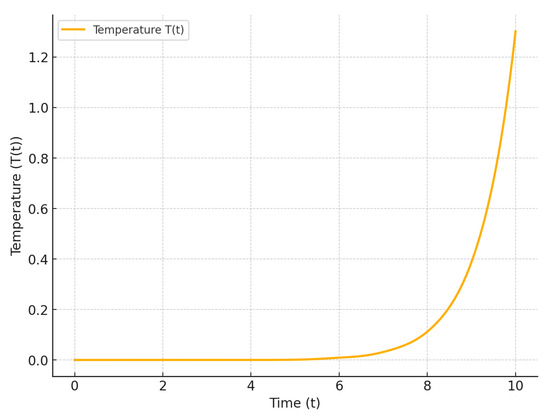
Figure 1. Nonoscillatory behavior of temperature $T\left(t\right)$ over time.

The simulation results, depicted in Figure 1, highlight the nonoscillatory behavior of the temperature control system under delayed feedback. The temperature stabilizes over time, demonstrating the validity of the sufficient conditions derived in this paper. The parameters $\alpha , \beta , \gamma , \zeta ,$ and $\omega$ significantly influence the stability and convergence of the system. For instance, increasing the feedback coefficient $r\left(t\right)$ or delay $\zeta$ could lead to oscillatory or unstable behavior, emphasizing the importance of parameter tuning in practical applications.

4. Conclusions

This study establishes new sufficient conditions for the existence of bounded nonoscillatory solutions to m-th-order neutral nonlinear differential equations with distributed deviating arguments. By applying Banach’s contraction principle, we extend and unify a number of earlier results in the literature, particularly those by Candan (2016) [13], Şenel et al. (2019) [14], and Cina et al. (2023) [15]. While prior works have mainly addressed first- or second-order cases with either pointwise or integral delays, our framework generalizes these findings by accommodating higher-order equations, more flexible classes of nonlinearities, and both discrete and distributed delays in a unified analytical setting. In addition, we address various scenarios for the neutral term, including positive, negative, and unbounded feedback functions, which increases the applicability of our results to a wider range of systems.

The practical relevance of the theoretical criteria is highlighted through an illustrative example involving a temperature control system with delayed feedback. Numerical simulations demonstrate the nonoscillatory behavior of the system, thereby validating the theoretical framework and showcasing its effectiveness in modeling real-world applications.

We note, however, that the numerical illustration provided focuses on a specific set of parameters chosen to highlight the theoretical findings in a representative case. We acknowledge the reviewer’s suggestion that more extensive simulations—such as bifurcation analysis or parameter sensitivity studies—could provide further insight into the dynamical behavior and robustness of the system. Such an in-depth numerical analysis remains a valuable direction for future research.

Future research may also explore generalizations involving state-dependent delays, stochastic effects, or hybrid dynamical systems. Additionally, the development of advanced numerical methods tailored to these types of equations could enhance the robustness and applicability of the theoretical results presented herein.

References

- Pontryagin, L.S. Mathematical Theory of Optimal Processes; Routledge: London, UK, 2018. [Google Scholar] [CrossRef]
- Rustichini, A. Hopf bifurcation for functional differential equations of mixed type. J. Dyn. Differ. Equ. 1989, 1, 145–177. [Google Scholar] [CrossRef]
- Slater, M.; Wilf, H.S. A class of linear differential-difference equations. Pacific J. Math. 1960, 10, 1419–1427. [Google Scholar] [CrossRef]
- Mallet-Paret, J. The global structure of traveling waves in spatially discrete dynamical systems. J. Dyn. Differ. Equ. 1999, 11, 49–127. [Google Scholar] [CrossRef]
- Mesmouli, M.B.; Hassan, T.S. On the positive solutions for IBVP of conformable differential equations. Aims Math. 2023, 8, 24740–24750. [Google Scholar] [CrossRef]
- Mesmouli, M.B.; Ardjouni, A.; Djoudi, A. Study of the periodic and nonnegative periodic solutions of functional differential equations via fixed points. Acta Universitatis Sapientiae Mathematica 2016, 6, 70–86. [Google Scholar] [CrossRef]
- Mesmouli, M.B.; Alesemi, M.; Mohammed, W.W. Periodic Solutions for a Neutral System with Two Volterra Terms. Mathematics 2023, 11, 1–8. [Google Scholar] [CrossRef]
- Mesmouli, M.B.; Menaem, A.A.; Hassan, T.S. Effectiveness of matrix measure in finding periodic solutions for nonlinear systems of differential and integro-differential equations with delays. Aims Math. 2024, 9, 14274–14287. [Google Scholar] [CrossRef]
- Mesmouli, M.B.; Khochemane, H.I. Theoretical study and numerical test for a delayed thermoelastic porous system with microtemperatures. ZAMM–J. Appl. Math. Mech. 2024, e202400123. [Google Scholar] [CrossRef]
- Candan, T. Nonoscillatory solutions of higher order differential and delay differential equations with forcing term. Appl. Math. Lett. 2015, 39, 67–72. [Google Scholar] [CrossRef]
- Candan, T. Existence of nonoscillatory solutions of higher-order nonlinear mixed neutral differential equations. Dyn. Syst. Appl. 2018, 27, 743–755. [Google Scholar] [CrossRef]
- Chen, M.P.; Yu, J.S.; Wang, Z.C. Nonoscillatory solutions of neutral delay differential equations. Bull. Aust. Math. Soc. 1993, 48, 475–483. [Google Scholar] [CrossRef]
- Candan, T.; Dahiya, R.S. Existence of nonoscillatory solutions of higher order neutral differential equations. Filomat 2016, 30, 2147–2153. [Google Scholar] [CrossRef]
- Şenel, M.T.; Candan, T.; Cina, B. Existence of nonoscillatory solutions of second-order nonlinear neutral differential equations with distributed deviating arguments. J. Taibah Univ. Sci. 2019, 13, 998–1005. [Google Scholar] [CrossRef]
- Cina, B.; Candan, T.; Senel, M.T. Existence of nonoscillatory solutions of higher order nonlinear neutral differential equations. Eur. J. Pure Appl. Math. 2023, 16, 713–723. [Google Scholar] [CrossRef]
- Slemrod, M. Nonexistence of oscillations in a nonlinear distributed network. J. Math. Anal. Appl. 1971, 36, 22–40. [Google Scholar] [CrossRef]
- Moaaz, O.; Dassios, I.; Bin Jebreen, H.; Muhib, A. Criteria for the nonexistence of Kneser solutions of DDEs and their applications in oscillation theory. Appl. Sci. 2021, 11, 425. [Google Scholar] [CrossRef]
- Moaaz, O.; Baleanu, D.; Muhib, A. New aspects for non-existence of kneser solutions of neutral differential equations with odd-order. Mathematics 2020, 8, 494. [Google Scholar] [CrossRef]
- Wong, J.S. Oscillation and nonoscillation of solutions of second order linear differential equations with integrable coefficients. Trans. Am. Math. Soc. 1969, 144, 197–215. [Google Scholar] [CrossRef]
- Elayaraja, R.; Kumar, M.S.; Ganesan, V. Nonexistence of Kneser solution for third order nonlinear neutral delay differential equations. In J. Phys. Conf. Ser. 2021, 1850, 012054. [Google Scholar] [CrossRef]
- Hassan, T.S.; Cesarano, C.; Mesmouli, M.B.; Zaidi, H.N.; Odinaev, I. Iterative Hille-type oscillation criteria of half-linear advanced dynamic equations of second order. Math. Methods Appl. Sci. 2024, 47, 5651–5663. [Google Scholar] [CrossRef]
- Hassan, T.S.; Bohner, M.; Florentina, I.L.; Abdel Menaem, A.; Mesmouli, M.B. New Criteria of oscillation for linear Sturm–Liouville delay noncanonical dynamic equations. Mathematics 2023, 11, 4850. [Google Scholar] [CrossRef]
- Hassan, T.S.; Moaaz, O.; Nabih, A.; Mesmouli, M.B.; El-Sayed, A.M. New sufficient conditions for oscillation of second-order neutral delay differential equations. Axioms 2021, 10, 281. [Google Scholar] [CrossRef]
- Agarwal, R.P.; Bazighifan, O.; Ragusa, M.A. Nonlinear neutral delay differential equations of fourth-order: Oscillation of solutions. Entropy 2021, 23, 129. [Google Scholar] [CrossRef] [PubMed]
- Bazighifan, O.; Ruggieri, M.; Scapellato, A. An improved criterion for the oscillation of fourth-order differential equations. Mathematics 2020, 8, 610. [Google Scholar] [CrossRef]
- Ahmad, S.; Ullah, A.; Partohaghighi, M.; Saifullah, S.; Akgül, A.; Jarad, F. Oscillatory and complex behaviour of Caputo-Fabrizio fractional order HIV-1 infection model. Aims Math. 2021, 7, 4778–4792. [Google Scholar] [CrossRef]
- Halanay, A. Differential Equations: Stability, Oscillations, Time Lags; Academic Press: Cambridge, MA, USA, 1966. [Google Scholar]
- El’sgol’ts, L.E. Introduction to the Theory of Differential Equations with Deviating Arguments; Academic Press: Cambridge, MA, USA, 1966. [Google Scholar]
- Hale, J.K.; Lunel, S.M.V. Introduction to Functional Differential Equations; Springer: Berlin/Heidelberg, Germany, 1993. [Google Scholar]
- MacDonald, N. Biological Delay Systems: Linear Stability Theory; Cambridge University Press: Cambridge, UK, 1989. [Google Scholar]
- Dugard, L. Stability and Control of Time-Delay Systems; Verriest, E.I., Ed.; Springer: London, UK, 1998; Volume 228. [Google Scholar]
Disclaimer/Publisher’s Note: The statements, opinions and data contained in all publications are solely those of the individual author(s) and contributor(s) and not of MDPI and/or the editor(s). MDPI and/or the editor(s) disclaim responsibility for any injury to people or property resulting from any ideas, methods, instructions or products referred to in the content. |
© 2025 by the authors. Licensee MDPI, Basel, Switzerland. This article is an open access article distributed under the terms and conditions of the Creative Commons Attribution (CC BY) license (https://creativecommons.org/licenses/by/4.0/).