Collision Detection Algorithms for Autonomous Loading Operations of LHD-Truck Systems in Unstructured Underground Mining Environments

Abstract

This study addresses collision detection in the unmanned loading of ore from load-haul-dump (LHD) machines into mining trucks in underground metal mines. Such environments present challenges like heavy dust, confined spaces, sensor occlusions, and poor lighting. This work identifies two primary collision risks and proposes corresponding detection strategies. First, for collisions between the bucket and tunnel walls, LiDAR is used to collect 3D point cloud data. The point cloud is processed through filtering, downsampling, clustering, and segmentation to isolate the bucket and tunnel wall. A KD-tree algorithm is then used to compute distances to assess collision risk. Second, for collisions between the bucket and the mining truck, a kinematic model of the LHD’s working device is established using the Denavit–Hartenberg (DH) method. Combined with inclination sensor data and geometric parameters, a formula is derived to calculate the pose of the bucket’s tip. Key points from the bucket and truck are then extracted to perform collision detection using the oriented bounding box (OBB) and the separating axis theorem (SAT). Simulation results confirm that the derived pose estimation formula yields a maximum error of 0.0252 m, and both collision detection algorithms demonstrate robust performance.

1. Introduction

The intelligentization of underground metal mining has been developing rapidly. Automation in fixed workstations has reached a relatively mature stage, and research on the intelligentization of mobile equipment is gaining increasing attention [1,2]. As a crucial piece of mining equipment, the load-haul-dump (LHD) machine plays a fundamental role in the intelligentization of mines, attracting considerable attention [3,4]. Some mining sites have already begun trial operations of remotely controlled LHDs [5,6]. However, research on the intelligentization of LHD operations in specific scenarios remains limited. For instance, achieving fully unmanned ore loading into mining trucks remains a significant challenge.

The ore loading process presents several safety hazards, including improper coordination between the LHD machine and the mining truck; falling ore during loading that may strike the truck body or the driver; collisions between the LHD machine, the mining truck, or the surrounding tunnel walls; and failure of operators to follow safety regulations. Additionally, the ore loading environment is typically complex, characterized by high noise levels and dust pollution, both of which can adversely affect workers’ health and safety [7]. Therefore, achieving unmanned ore loading is of great significance in reducing workplace accidents and enhancing operational safety.

When the LHD machine and the mining truck operate in narrow and complex underground tunnels, collision risks exist in addition to the dangers posed by manual operation. Therefore, to successfully achieve unmanned ore loading, it is essential to fully account for potential collisions. Developing a collision detection algorithm tailored to the underground mining environment and the ore loading process is thus crucial. This algorithm must be capable of issuing timely warnings before potential collisions occur and guiding the control system to make necessary adjustments to ensure operational safety.

Collision detection refers to the process of determining whether two or more objects come into contact at one or more points. Current research in collision detection addresses the trade-off between accuracy and efficiency through several principal methodologies. An initial distinction often arises from sensor modality. Although vision-based detection systems demonstrate advantages in open environments [8,9,10,11,12], the challenges posed by light attenuation and dust interference in underground mining conditions have led researchers to explore LiDAR point cloud data as an alternative solution.

One prominent trajectory, model-based detection, circumvents external sensors by monitoring a system’s intrinsic dynamics. Foundational methods infer collisions from discrepancies between predicted and measured motor torque [13], while more advanced techniques use sophisticated observers to estimate external forces with greater sensitivity [14]. This approach has been further enhanced by integrating neural networks to compensate for complex nonlinearities like friction [15] or to serve as powerful classifiers within a momentum-observer framework [16]. Innovations in signal processing using “envelope-like lines” [17] and time-series analysis (TSA) [18] have also pushed the boundaries of creating a truly sensorless detection paradigm.

In parallel, the classical geometry-centric paradigm provides high-fidelity detection founded upon geometric representations. This approach is dominated by bounding volume hierarchies (BVHs), which use a variety of primitives—from simple spheres [19] to complex, application-tailored hybrid models combining shapes like ellipsoidal bounding boxes (EBBs), oriented bounding boxes (OBBs), and capsules [20,21,22]. The fidelity of these hierarchies is continually refined through improved axis-aligned bounding box (AABB) structures [23] and advanced node calculation methods [24]. To handle unstructured data from sensors like LiDAR, these methods are often augmented with spatial partitioning techniques such as KD-trees [25] and octrees [26] or voxel-based representations [27,28]. This can involve representing objects as “stretched primitives” [29] or employing multi-stage pipelines that sequentially filter and segment point clouds before generating bounding boxes [30,31]. Further innovations enhance performance through techniques like dual-resolution depth maps [32], depth-buffer comparison [33], and novel data structures [34]. Other works reformulate the problem entirely, using signed distance functions (SDFs) [35] or pseudodistance metrics [36] to improve efficiency.

More recently, a paradigm shift toward data-driven and AI approaches seeks to overcome the limitations of explicit modeling. End-to-end frameworks like CollisionNet learn to recognize collisions directly from sensor signals [37], while hybrid models such as DLGJK synergize the speed of deep learning for coarse checks with the precision of classical algorithms like the Gilbert–Johnson–Keerthi (GJK) for fine-level verification [38].

Complementing these core methodologies is a significant body of research focused on system-level and algorithmic optimization. This includes enhancing broad-phase algorithms like sweep-and-prune with temporal inference [39] or kinetic, event-driven mechanisms [40]. Hardware acceleration is another critical vector, leveraging GPU pipelines [41] and parallelization techniques like SIMD-KD trees [42]. In parallel, memory optimization is addressed through novel BVH representations with binary encodings [43] and specialized architectures like QuickNN that tackle memory bandwidth bottlenecks [44]. The research scope has also broadened beyond simple binary checks to include probabilistic methods for both general and specific applications [45,46], acceleration techniques that identify high-probability “feature points” [47], and algorithms designed to improve iterative efficiency [48]. This trend toward specialization is further underscored by custom data structures for high-resolution models [49] and tailored strategies for specific industrial machinery [50] or internal components like flexible joints [51].

In summary, significant progress has been made in the research of collision detection algorithms, with most efforts focused on improving algorithm efficiency and theoretical foundations. However, there has been little attention given to collision detection specifically for the operational scenarios of underground mining shovels. The mining operations studied in this paper are conducted in underground metal mining environments, which are characterized by heavy dust, confined spaces, and complex lighting conditions, making visual sensors such as cameras unsuitable. During the ore loading operation, the boom of the LHD needs to be lifted, which can obstruct the sensors and lead to missing scan data. Therefore, it is essential to develop an efficient and safe collision detection system specifically designed for unmanned ore loading in view of the complex underground environment and the possible collision situation during ore loading operation.

This study was conducted on the basis that both the LHD machine and the mining truck have already achieved autonomous operation. The potential collisions during the ore loading process were classified into two scenarios. The first scenario involves a collision between the bucket and the tunnel wall during the boom’s lifting process, while the second scenario concerns a collision between the bucket and the mining truck when dumping ore. For the first scenario, the point cloud data collected by the LiDAR were first processed using distance filtering and voxel downsampling. Then, the density-based spatial clustering of applications with noise (DBSCAN) algorithm was applied for clustering, and finally, collision detection was performed using nearest neighbor search based on the KD-tree. For the second scenario, the Denavit–Hartenberg (DH) parameter method was used to establish the kinematic model of the LHD’s working device, and the mathematical formula for calculating the bucket tooth tip pose was derived. Based on the geometric shapes of the bucket and the mining truck, an appropriate OBB was constructed. Collision detection was then conducted using the separating axis theorem (SAT). Finally, experiments were conducted in a simulated environment. The results demonstrate that the proposed pose calculation formula and collision detection algorithm are effective and feasible, well-suited for underground mining environments and ore loading operations. The complete workflow integrating these two approaches and their experimental validation is visually summarized in Figure 1.

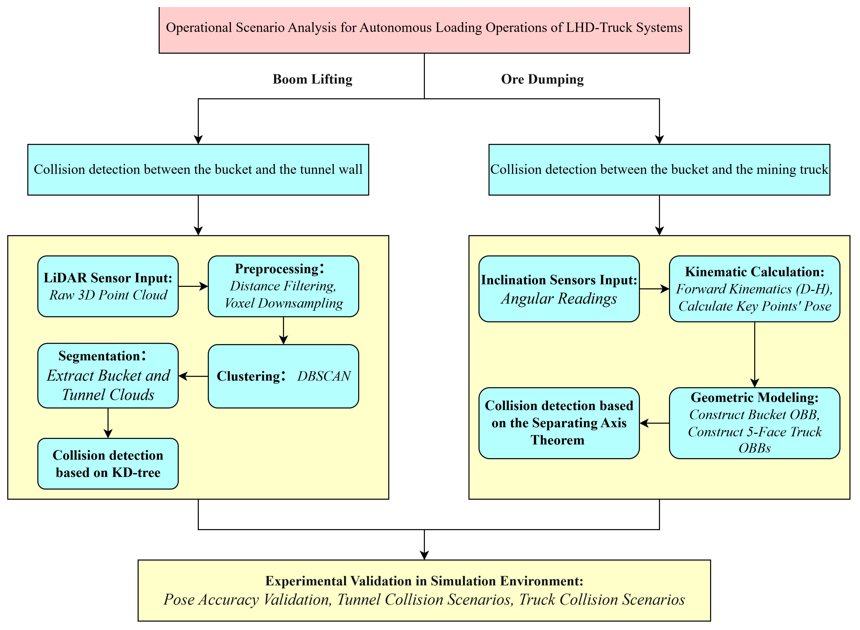
2. Materials and Methods

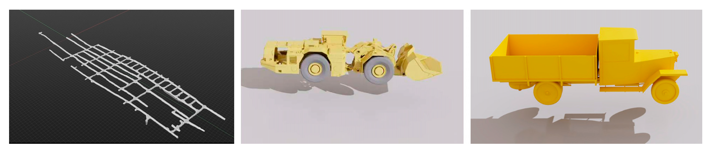
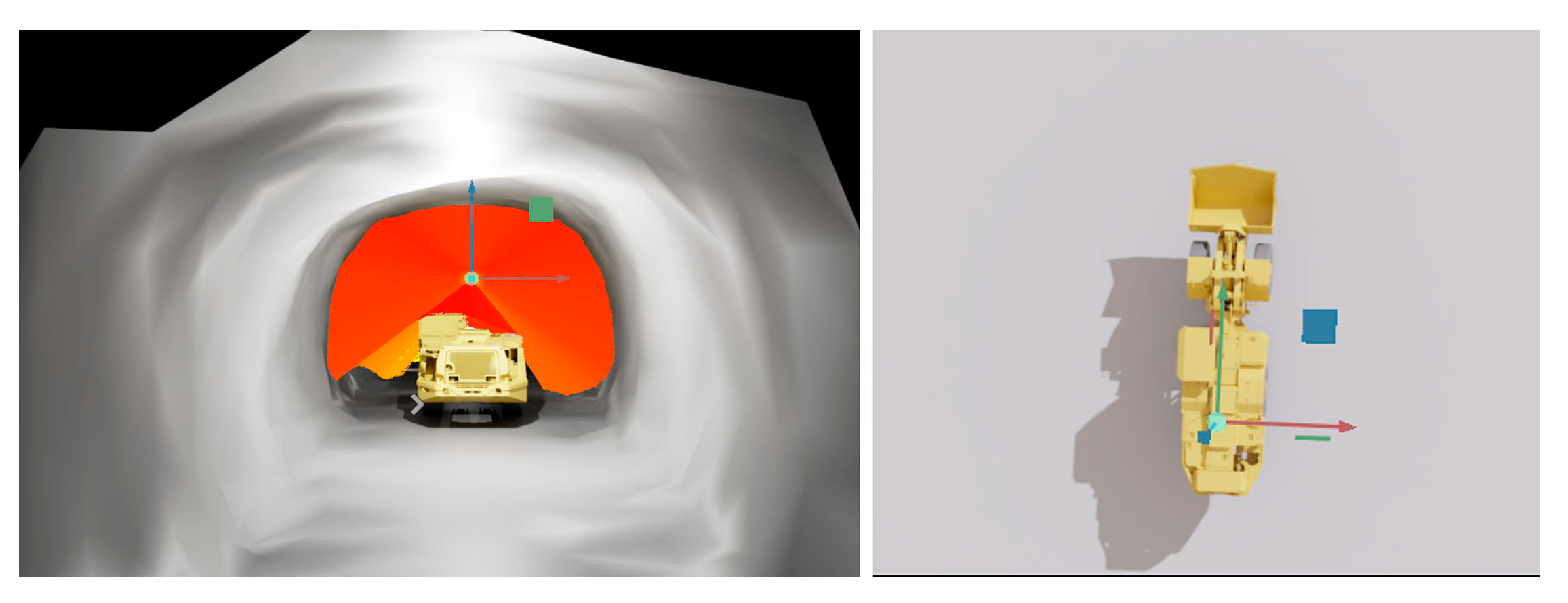
2.1. Construction of a Simulation Environment for Ore Loading Operations in Underground Metal Mines

A realistic simulation environment representing an underground metal mine was constructed on the Isaac Sim platform. Isaac Sim, a physics-based robotics simulation platform developed by NVIDIA, was engineered to accelerate the development and testing of robots and automation systems. This platform features a high-fidelity physics engine and supports the entire robotics development lifecycle, from conceptual design to deployment. The simulation was executed on a workstation equipped with an Intel(R) Core(TM) i7-10700K CPU @ 3.80GHz (Intel Corporation, Santa Clara, CA, USA) and an NVIDIA GeForce RTX 2060 SUPER GPU (NVIDIA Corporation, Santa Clara, CA, USA) and running the Ubuntu 20.04 operating system.

As depicted in Figure 2, the simulation environment comprises three primary components: a tunnel, an LHD machine, and a mining truck. The LHD’s operational movements, which include linear translation (forward/backward), turning, boom actuation (lifting/lowering), and bucket tilting, were controlled via Python scripting. These scripted actions enable the simulation of the complete ore loading process from the LHD to the mining truck. The version of Python used in our research is Python 3.10.15.

2.2. LiDAR-Based Collision Detection Between the Bucket and the Tunnel

The ore loading process, which involves transferring material from an LHD machine to a mining truck, necessitates the preliminary lifting of the LHD’s boom. As the boom ascends within the confined space of an underground tunnel, the risk of collision between the bucket and the tunnel walls increases significantly. Such collisions can lead to spillage of ore and pose considerable safety hazards. To mitigate this risk, this study proposes a method that utilizes LiDAR to acquire 3D point cloud data of the operating environment, encompassing both the tunnel walls and the LHD bucket. The acquired point cloud data are then processed through a sequential pipeline of filtering, downsampling, clustering, and segmentation. Finally, collision risk is assessed by performing a nearest-neighbor search, accelerated by a KD-tree data structure.

2.2.1. LiDAR Installation Position and Data Acquisition

Since both the tunnel and the bucket need to be detected simultaneously during boom lifting, it is essential to select a LiDAR with a large vertical field of view and carefully consider its installation position. In this study, a multi-line mechanical LiDAR is used, featuring a horizontal field of view of 120° and a vertical field of view of 60°. It is installed at a height of 2.8 m from the chassis of the LHD. The LiDAR position and scanning range are shown in Figure 3.

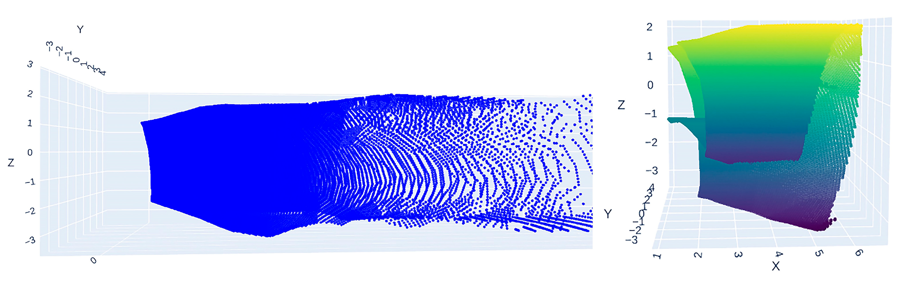
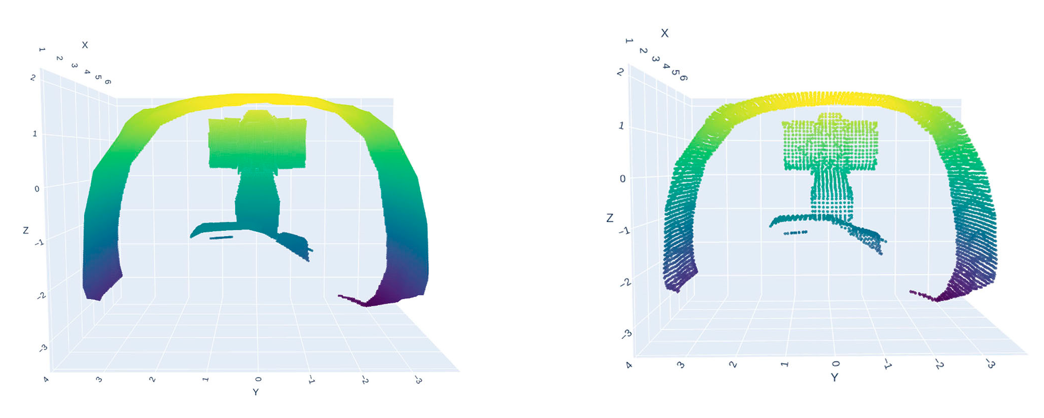
2.2.2. Point Cloud Preprocessing

The raw point cloud data collected from the LiDAR are typically large and dense; therefore, a preprocessing stage is essential to facilitate efficient subsequent processing. This stage consists of two primary steps. The first step involves a distance-based filtering to remove points located far from the LiDAR sensor, which are irrelevant to collision detection and unnecessarily increase the computational load for subsequent stages. The second step is voxel grid downsampling, a technique that reduces point cloud density while preserving the overall geometric structure without significant alteration. This reduction in data volume decreases the computational time for subsequent algorithms, a crucial factor for achieving real-time performance.

A key parameter in the distance filtering process is the maximum range threshold. This threshold was set to 7 m, a value determined based on the LHD’s dimensions and its effective operational envelope. During the loading cycle, points beyond this range are considered irrelevant for imminent collision detection, so this filtering step effectively isolates the region of interest and significantly reduces the computational load for subsequent stages. The result of this filtering step is visualized in Figure 4.

In voxel downsampling, the 3D space is partitioned into a grid of cubic cells known as voxels. The principle of this method is to replace all points contained within each non-empty voxel with a single representative point. Typically, this representative point is the centroid (average) of the contained points. Voxel downsampling is computationally efficient and promotes a more uniform spatial distribution of points. The voxel size parameter directly controls the sparsity of the output point cloud. In this study, a voxel size of 0.1 m was used. This value represents a carefully considered trade-off between preserving sufficient geometric detail and ensuring real-time performance. Our empirical tests within the simulation environment confirmed that 0.1 m provides the optimal balance for this application, as a smaller size would increase computational cost unnecessarily, while a larger size could risk over-simplifying critical geometric features. The result of the voxel downsampling is illustrated in Figure 5.

By applying these two preprocessing steps, extraneous points are eliminated, enabling the collision detection algorithm to focus on the relevant target area. The significant reduction in the point count decreases the computational load and accelerates the algorithm’s execution. Furthermore, key geometric features are preserved, and the point distribution becomes more uniform, ensuring that subsequent clustering algorithms can operate effectively and yield accurate results.

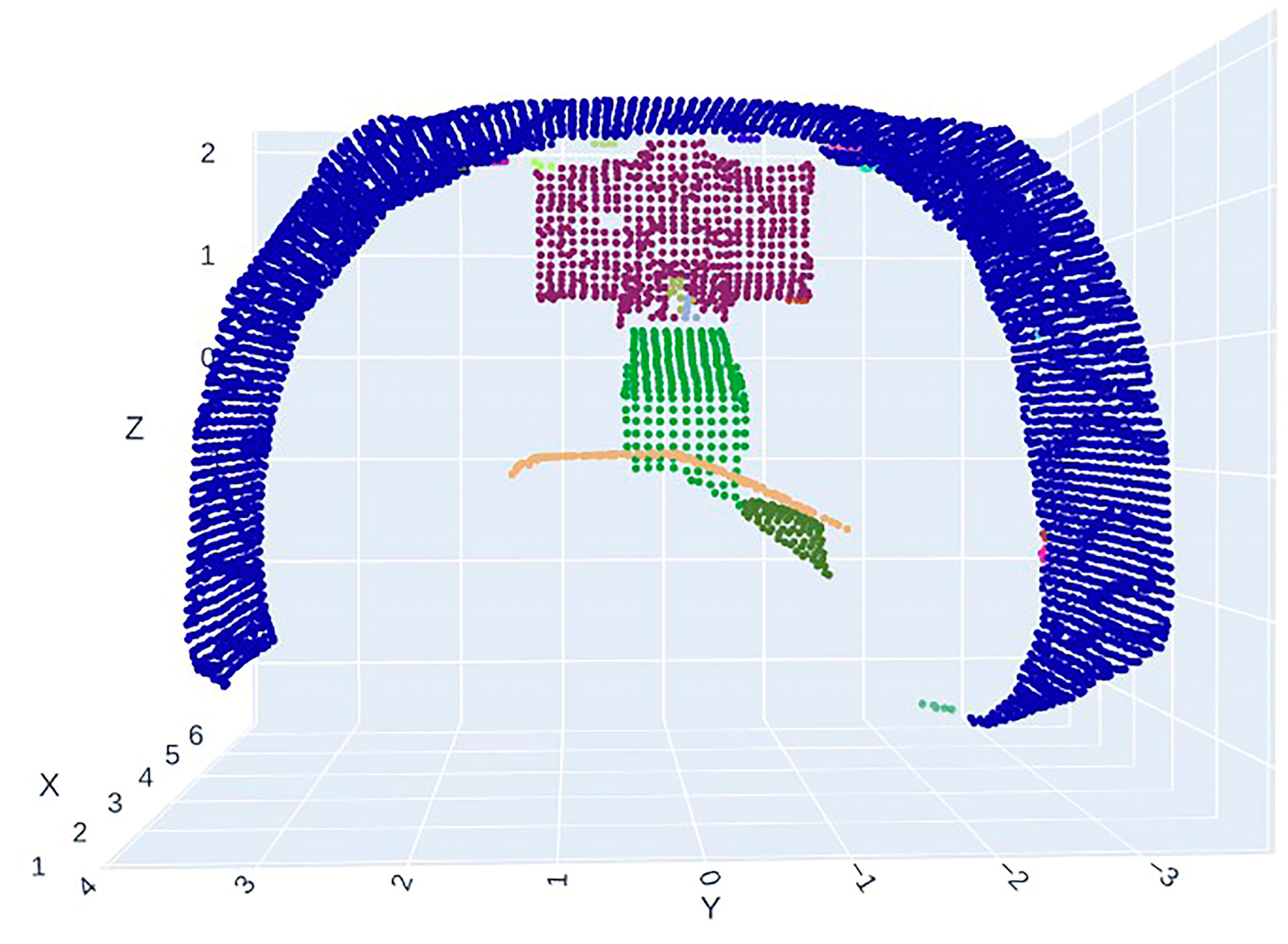
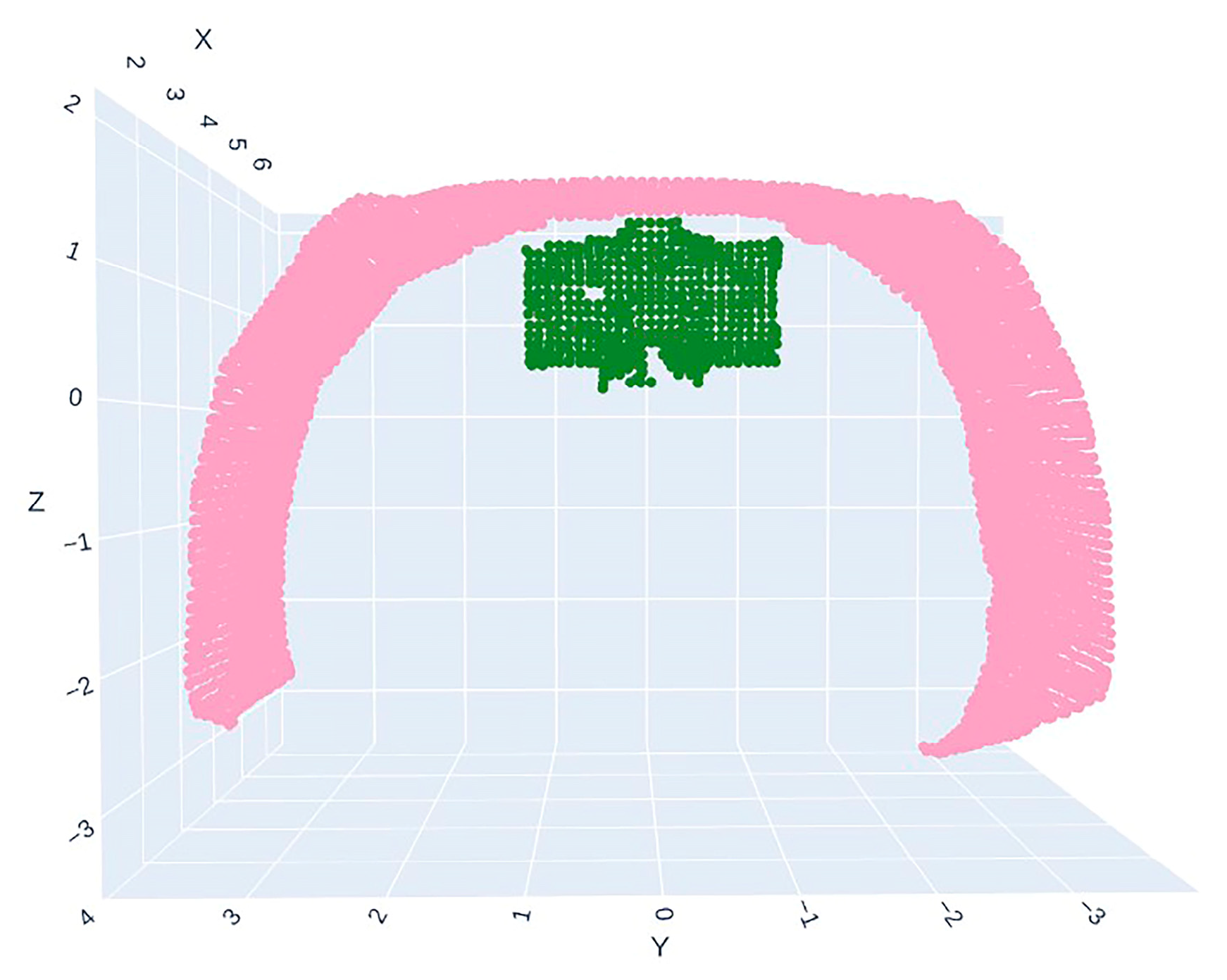
2.2.3. Point Cloud Clustering and Segmentation

Point cloud clustering is the process of partitioning a point cloud dataset into distinct subsets, i.e., clusters, based on specific similarity criteria. Typically, points within a given cluster exhibit high similarity (e.g., spatial proximity), whereas points in different clusters are dissimilar.

The point cloud data collected by the LiDAR present several challenges that necessitate a sophisticated clustering approach. The data contain not only the intended targets (the bucket and tunnel) but also other components of the LHD, which manifest as noise or distinct objects. Furthermore, dynamic movements, such as the boom being raised, cause partial occlusions that alter the scanned area and data density. Consequently, the number and shape of object clusters are unknown and cannot be predetermined.

To address these conditions—namely the presence of noise, arbitrarily shaped clusters, and an unknown number of clusters—we employ the classical DBSCAN algorithm, as originally proposed by Ester et al. [52]. This method is particularly well-suited for our task because it identifies clusters based on local point density. Its core idea is to define clusters as high-density regions separated by areas of low density. This density-driven approach allows DBSCAN to effectively distinguish meaningful object clusters from sparse noise and discover clusters of arbitrary shapes, all without requiring the number of clusters as a predefined input.

The principles of DBSCAN can be described through the following core concepts:

1.

Core point: A point is considered a core point if its neighborhood (i.e., within a radius $\epsilon$) contains at least $minPts$ points. In other words, the density around the point is greater than or equal to $minPts$;

2.

Border point: A point is located within the neighborhood of another core point, but it is not itself a core point. Specifically, its neighborhood contains fewer than $minPts$ points, but it belongs to the neighborhood of a core point;

3.

Noise point: A point that is neither a core point nor a border point. It does not belong to any cluster and is typically considered an outlier or noise;

4.

Neighborhood: Given a point $p$, its neighborhood refers to all points within a radius $\epsilon$ of $p$.

The performance of DBSCAN is highly dependent on the choice of two key parameters: the neighborhood radius ($\epsilon$) and the minimum number of points ($minPts$). In this study, these parameters were determined through extensive empirical testing within our simulation environment to find the optimal values for our specific application.

We ultimately set $\epsilon$ to 0.11 m and $minPts$ to 4. The rationale for these specific values is as follows: The 0.11 m radius is slightly larger than our voxel grid size (0.1 m), which ensures that points on the same object surface, even if located in adjacent voxels, can be robustly connected into a single cluster. This value is also small enough to maintain a clear distinction between the bucket and tunnel wall during close-approach scenarios, thus preventing erroneous cluster merging. The $minPts$ value of 4 was found to be sufficient to identify the surfaces of our key objects after downsampling while still effectively filtering out isolated noise points. This combination provided the best balance between clustering sensitivity and noise immunity in our tests.

DBSCAN forms clusters by connecting neighboring points based on density. If a point is a core point, and there are other points within its neighborhood, these points will be connected to form a cluster. This process continues iteratively until the entire cluster is expanded. Points that cannot be connected to any cluster are considered noise. The clustered point cloud is shown in Figure 6.

The next step involves segmenting the output of the clustering algorithm to isolate the point clouds corresponding to the bucket and the tunnel wall for subsequent collision detection. Based on the a priori knowledge that the tunnel wall and bucket are the largest objects in the scene, the clusters are sorted by point count, and the two largest clusters are extracted. The final segmented point cloud, containing only the two target clusters, is shown in Figure 7.

2.2.4. Collision Detection Based on KD-Tree

A KD-ree is a space-partitioning data structure, organized as a binary tree, for storing points in a K-dimensional space. It enables efficient nearest-neighbor searches by recursively partitioning the space into nested regions. Each node in the tree corresponds to a data point and defines a hyperplane that splits the space into two half-spaces, represented by its child nodes. The splitting dimension typically cycles through the coordinates as the tree depth increases, distributing points into left and right subtrees. In collision detection, the process involves querying the nearest-neighbor distance between points in one point cloud and those in another to determine whether a collision has occurred.

In this section, we aim to detect whether the bucket has collided with the tunnel. The algorithm for implementing this collision detection is outlined as follows:

1.

Constructing the KD-tree: Build a KD-tree for the tunnel point cloud. This process partitions the space and organizes the tunnel point cloud into a tree structure;

2.

Setting the collision threshold: Define a $distance\_threshold$ to determine whether two points are considered to be in collision;

3.

Iterating through the bucket point cloud: For each point in the bucket point cloud, use the KD-tree to query the nearest point in the tunnel point cloud;

4.

Computing the Euclidean distance: Calculate the Euclidean distance between the query point $P_2$ and its nearest neighbor $P_1$ in the tunnel point cloud using the formula

$$d\left(P_1,P_2\right)=\sqrt{{\left(x_2 -x_1\right)}^2+{\left(y_2 -y_1\right)}^2+{\left(z_{2 }-z_1\right)}^2}$$

(1)

where $P_1 =\left(x_1 ,y_1,z_1\right)$ and $P_2=\left(x_2,y_2,z_2\right)$ are the coordinates of the two points;

5.

Querying the nearest neighbor: Utilize the KD-tree to search for the nearest neighbor in the tunnel point cloud. The query process can be represented using the following formula:

$$neares{t}_{neighbor\left(P_2\right)}=arg\min \hspace{0.33em} d\left(P_1,P_2\right)$$

(2)

$P_2$ is the query point from the bucket point cloud, while $P_1$ is the nearest point to $P_2$ found in the KD-tree, originating from the tunnel point cloud. The Euclidean distance between them is denoted as $d\left(P_1,P_2\right)$;

6.

Collision determination: If the computed distance is smaller than the predefined threshold ($distance\_threshold$), a collision is considered to have occurred:

$$d\left(P_1,P_2\right)<distance\_threshold$$

(3)

where $d\left(P_1,P_2\right)$ represents the Euclidean distance between $P_1$ and $P_2$, and $distance\_threshold$ is the predefined distance threshold.

If the distance between any pair of points is smaller than the threshold, a collision alert is triggered. If all points are checked and no collision is detected, the algorithm concludes that no collision has occurred.

The complete algorithmic workflow, presented as pseudocode, is divided into two main parts. Algorithm 1 details the point cloud preprocessing stage, which includes distance-based filtering and voxel grid downsampling. Algorithm 2 describes the subsequent pipeline for clustering, segmentation, and collision detection. This algorithm first clusters the point cloud using DBSCAN (with parameters $\epsilon$ and $minPts$), then segments the two largest clusters (the tunnel and bucket). Finally, it computes the minimum distance between these two clusters to determine if it falls below the predefined collision threshold.

Algorithm 1: PointCloudPreprocessor
	Input:   P_raw, The raw point cloud from the LiDAR sensor;   d_max, The maximum distance threshold for filtering. (e.g., 7 m);   v_size, The voxel size for downsampling. (e.g., 0.1).
	Output:   P_processed, The preprocessed (filtered and downsampled) point cloud.
1	function PreprocessPointCloud(P_raw, d_max, v_size):
2	// Step 1: Filter by Distance
3	P_filtered ← an empty point cloud
4	for each point p in P_raw:
5	dist ← Calculate Euclidean distance of p from the origin
6	if dist < d_max then
7	P_filtered ← P_filtered ∪ {p}
8	end if
9	end for
10	// Step 2: Voxel Grid Downsampling
11	P_processed ← VoxelGridDownsample(P_filtered, v_size)
12	return P_processed
13
14	function VoxelGridDownsample(P_in, voxel_size):
15	Create a voxel grid with resolution voxel_size over P_in
16	P_out ← an empty point cloud
17	for each non-empty voxel v in the grid:
18	p_centroid ← Compute the centroid of all points within v
19	P_out ← P_out ∪ {p_centroid}
20	end for
21	return P_out

Algorithm 2: DBSCAN Clustering and Collision Detection
	Input:   P_in, a preprocessed point cloud;   eps, DBSCAN radius;   min_pts, DBSCAN minimum points;   N, number of clusters to select;   τ, collision threshold.
	Output:   CollisionAlert, a boolean value.
1	function ClusterAndCheckCollision(P_in, eps, min_pts, N, τ):
2	// Step 1: Point Cloud Clustering
3	labels ← DBSCAN(P_in, eps, min_pts)
5	// Step 2: Select Largest Clusters
6	all_clusters ← Group points from P_in by labels (excluding noise)
7	Sort all_clusters by size in descending order
8	largest_clusters ← Select top N clusters from all_clusters
9	C_tunnel ← largest_clusters[0]
10	C_bucket ← largest_clusters[1]
12	// Step 3: Collision Detection
13	kd_tree ← BuildKDTree(C_tunnel)
14	for each point p in C_bucket:
15	dist ← FindNearestNeighborDistance(p, kd_tree)
16	if dist < τ then
17	return True // Collision detected
18	end if
19	end for
20
21	return False // No collision detected

2.3. Collision Detection Algorithm Based on the Pose of Key Points on the Bucket

During ore loading operations, there is a significant risk of collision between the LHD bucket and the mining truck. Such incidents can disrupt the operational workflow, cause equipment damage, and pose considerable safety risks. Therefore, it is crucial to detect potential collisions between the bucket and the mining truck. However, during the loading process, due to the lifting and lowering of the boom as well as the retraction and tilting of the bucket and the limited installation positions of sensors, the scanning range of the sensors may be obstructed, preventing them from fully capturing the bucket and the mining truck. In this case, the sensors are ineffective. This section establishes a DH kinematic model for the LHD’s working device and uses forward kinematics to calculate the precise pose of the bucket’s tip. Based on the geometric parameters of the bucket, the poses of key points on the bucket are then derived, and an OBB is constructed. For the mining truck, the poses of key points are derived based on the pose of the truck’s sensors and its geometric parameters. An OBB is constructed for each face of the truck. The OBB of the bucket is then checked for collisions with the OBB of each face of the truck using the SAT.

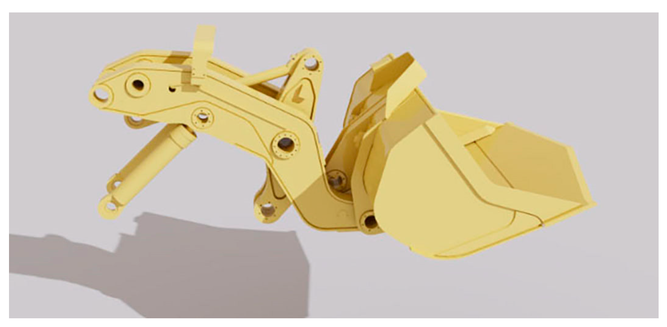
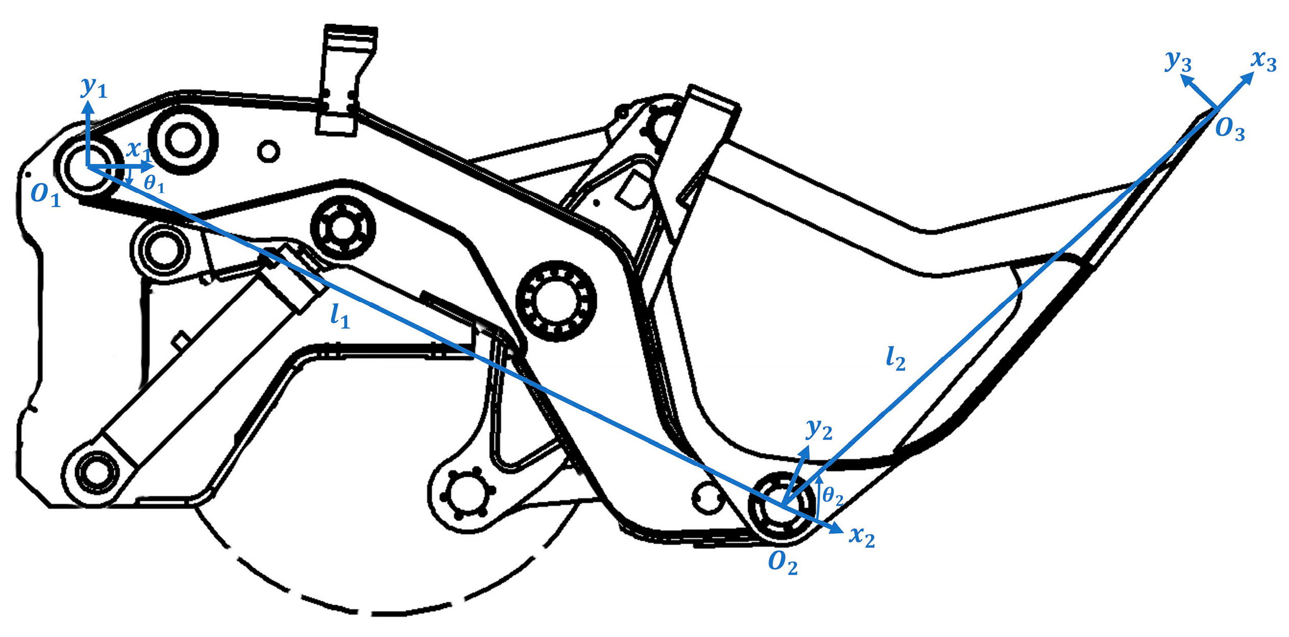
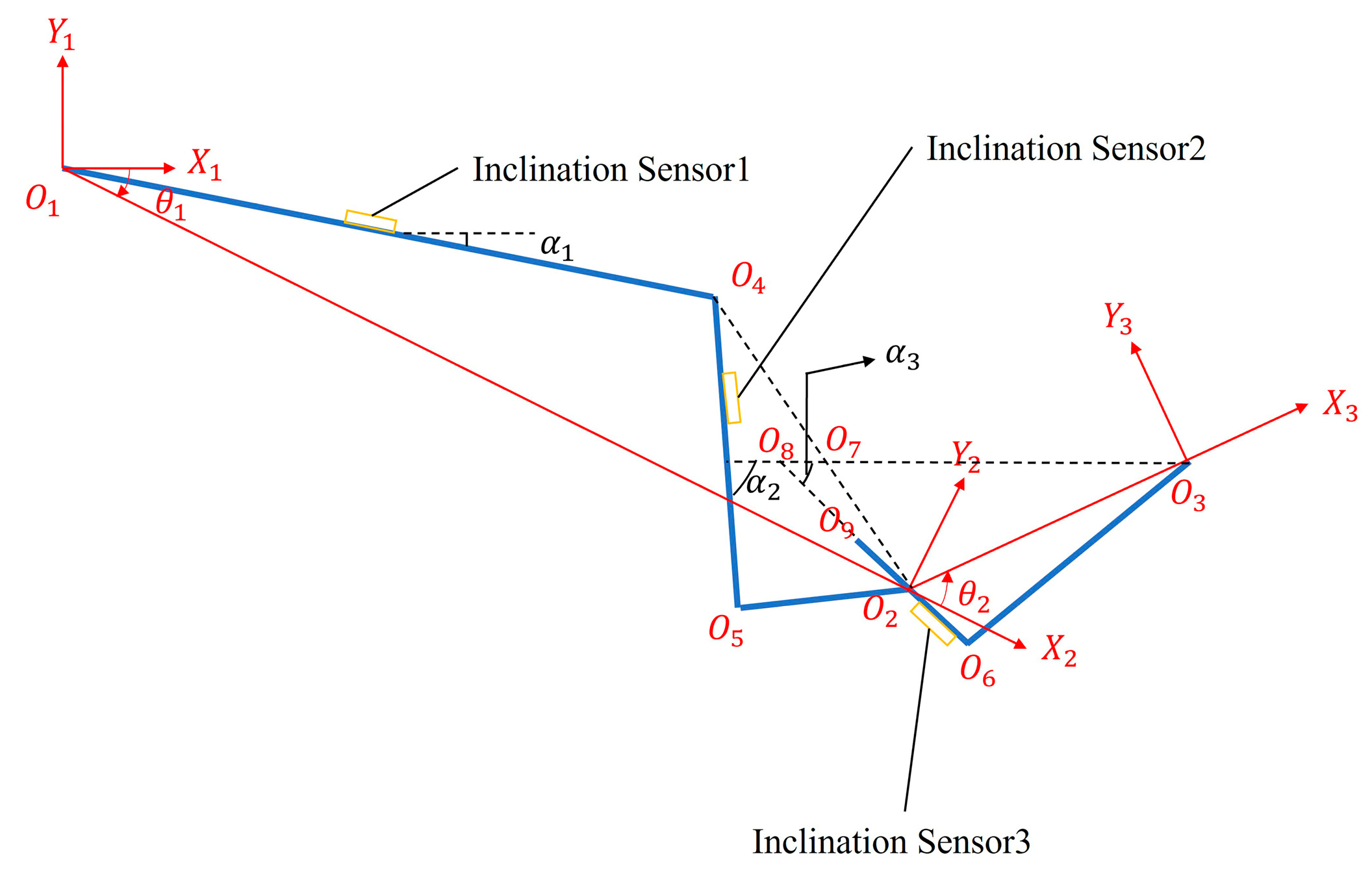
2.3.1. Kinematic Model of the LHD’s Working Device

The main components of the LHD’s working device consist of the boom, bucket, and other mechanisms such as the hydraulic cylinder, rocker, and linkage, as shown in Figure 8.

Robot kinematics is a field of study concerned with the motion of robotic manipulators, encompassing both forward and inverse kinematics. Forward kinematics solves for the pose (position and orientation) of the end-effector given a set of known joint variables. Conversely, inverse kinematics determines the required joint variables to achieve a desired end-effector pose. In forward kinematics, the spatial relationship between adjacent links is described by a homogeneous transformation matrix, representing six degrees of freedom (three translational and three rotational). By sequentially multiplying these transformation matrices from the base to the end-effector, the forward kinematic chain is computed, yielding the end-effector’s pose relative to the base coordinate system.

The DH parameter model is a widely used standardized method for representing and describing the relationships between the joints and links of a robotic arm. It uses a set of four parameters to represent the relative position and orientation of each joint and link in the robotic arm [53].

The core principle of the DH model is to define the spatial relationship between two consecutive links, using a minimal set of four parameters:

1.

${\theta }_i$: Joint angle (rotation angle), which represents the rotation of the previous link relative to the current link around the $Z_{i-1}$ axis. This parameter is typically associated with the rotation of the joint, with clockwise rotation defined as negative and counterclockwise rotation as positive;

2.

$d_i$: Link offset (translation), which represents the displacement of the current link along the $Z_{i-1}$ axis. This parameter is typically associated with the displacement of the joint;

3.

$a_i$: Link length, which represents the distance between the previous and current links along the $X_i$ axis. This parameter describes the fixed length between the links;

4.

${\alpha }_i$: Link twist angle, which represents the rotation of the previous link relative to the current link around the $X_i$ axis.

Using these four parameters, a 4 × 4 transformation matrix can be constructed to describe the relative transformation from the coordinate frame of $lin{k}_{i-1}$ to the coordinate frame of $lin{k}_i$. The transformation matrix ($T_{i-1}^i$) for each joint can be represented as

$$T_{i-1}^i=\left[\begin{array}{cccc}\cos \left({\theta }_i\right)& -\sin \left({\theta }_i\right)\cdot \cos \left({\alpha }_i\right)& \sin \left({\theta }_i\right)\cdot \sin \left({\alpha }_i\right)& a_i\cdot \cos \left({\theta }_i\right)\\ \sin \left({\theta }_i\right)& \cos \left({\theta }_i\right)\cdot \cos \left({\alpha }_i\right)& -\cos \left({\theta }_i\right)\cdot \sin \left({\alpha }_i\right)& a_i\cdot \sin \left({\theta }_i\right)\\ 0& \sin \left({\alpha }_i\right)& \cos \left({\alpha }_i\right)& d_i\\ 0& 0& 0& 1\end{array}\right]$$

(4)

By sequentially multiplying these individual transformation matrices, the total transformation matrix from the base frame to the end-effector frame, $T_0^n$, can be computed as

$$T_0^n=T_0^1\cdot T_1^2\cdot \cdots \cdot T_{n-1}^n$$

(5)

Using this matrix, the position and orientation of the end effector can be determined, enabling kinematic analysis and control. The coordinate systems of each link in the LHD’s working mechanism, established using the DH modeling method, are shown in Figure 9.

1.

$O_1$, $O_2$, and $O_3$ represent the origins of the three coordinate systems. $O_1$ is the articulation point between the boom and the base, $O_2$ is the articulation point between the bucket and the boom, and $O_3$ is located at the tip of the bucket;

2.

The $z_1$, $z_2$, and $z_3$ axes are parallel and perpendicular to the $O_1{X}_1{Y}_1$ plane;

3.

The $X_1$ axis is along the reference horizontal plane, the $X_2$ axis points in the direction of $O_1{O}_2$, and the $X_3$ axis points in the direction of $O_2{O}_3$.

The resulting DH parameters for the LHD’s working device are summarized in

Table 1. Represents the length between $O_1$ and $O_2$, $l_2$ denotes the length between $O_2$ and $O_3$, ${\theta }_1$ is the angle between $O_1{O}_2$ and $O_1{X}_1$, and ${\theta }_2$ is the angle between $O_2{X}_2$ and $O_2{O}_3$.

Link $\mathit{i}$	${\mathit{\theta }}_{\mathit{i}}$	${\mathit{d}}_{\mathit{i}}$	${\mathit{a}}_{\mathit{i}}$	${\mathit{\alpha }}_{\mathit{i}}$
2	${\theta }_1$	0	$l_1$	0
3	${\theta }_2$	0	$l_2$	0

.

2.3.2. Forward Kinematics Analysis

Based on the previously established DH parameter model, the homogeneous transformation matrices between adjacent joints of the LHD’s working device are computed.

$$T_1^2=\left[\begin{array}{cccc}\cos \left({\theta }_1\right)& -\sin \left({\theta }_1\right)& 0& l_1\cdot \cos \left({\theta }_1\right)\\ \sin \left({\theta }_1\right)& \cos \left({\theta }_1\right)& 0& l_1\cdot \sin \left({\theta }_1\right)\\ 0& 0& 1& 0\\ 0& 0& 0& 1\end{array}\right]$$

(6)

$$T_2^3=\left[\begin{array}{cccc}\cos \left({\theta }_2\right)& -\sin \left({\theta }_2\right)& 0& l_2\cdot \cos \left({\theta }_2\right)\\ \sin \left({\theta }_2\right)& \cos \left({\theta }_2\right)& 0& l_2\cdot \sin \left({\theta }_2\right)\\ 0& 0& 1& 0\\ 0& 0& 0& 1\end{array}\right]$$

(7)

By multiplying these matrices, the total transformation from the base frame $O_1$ to the bucket tip frame $O_3$ is obtained as shown in Equation (8):

$$T_1^3=T_1^2\cdot T_2^3 =\left[\begin{array}{cccc}\cos \left({\theta }_1+{\theta }_2\right)& -\sin \left({\theta }_1+{\theta }_2\right)& 0& l_2\cdot \cos \left({\theta }_1+{\theta }_2\right)+l_1\cdot \cos \left({\theta }_1\right)\\ \sin \left({\theta }_1+{\theta }_2\right)& \cos \left({\theta }_1+{\theta }_2\right)& 0& l_2\cdot \sin \left({\theta }_1+{\theta }_2\right)+l_1\cdot \sin \left({\theta }_1\right)\\ 0& 0& 1& 0\\ 0& 0& 0& 1\end{array}\right]$$

(8)

From this transformation matrix, the coordinates of the bucket tip in the base coordinate system are extracted as presented in the equations below:

$$\left\{\begin{array}{l}{x}_3=l_2\cdot cos\left({\theta }_1+{\theta }_2\right)+l_1\cdot cos\left({\theta }_1\right)\hfill \\ y_3=l_2\cdot sin\left({\theta }_1+{\theta }_2\right)+l_1\cdot sin\left({\theta }_1\right)\hfill \\ z_3=0\hfill \end{array}\right.$$

From the above equation, it can be seen that by knowing ${\theta }_1$, ${\theta }_2$, $l_1$, and $l_2$, the pose corresponding to the bucket tip of the LHD can be determined. $l_1$ and $l_2$ are fixed parameters of the LHD and remain constant. Therefore, only the rotation angles ${\theta }_1$ and ${\theta }_2$ of the boom and bucket joints need to be calculated.

To facilitate this calculation, a simplified kinematic model of the LHD’s working device is introduced, as illustrated in Figure 10.

The measurement value of the inclination sensor represents the angle between its body and the horizontal direction, with positive values indicating an upward inclination and negative values indicating a downward inclination. Inclination Sensor1 is installed along the line connecting the boom pivot point $O_1$ and the rocker pivot point $O_4$, with the measurement denoted as ${\alpha }_1$. Inclination Sensor2 is installed along the direction of $O_4{O}_5$, with the measurement denoted as ${\alpha }_2$. Inclination Sensor3 is installed along the direction of $O_2{O}_6$, with the measurement denoted as ${\alpha }_3$.

The first step is to calculate the boom’s rotation angle (${\theta }_1$). ${\theta }_1$ represents the angle between $O_1{O}_2$ and the $O_1{X}_1$ axis.

$${\theta }_1={\alpha }_1-\angle O_2{O}_1{O}_4$$

(9)

In triangle $O_2{O}_1{O}_4$, the side lengths of this triangle are fixed structural parameters of the LHD. Using the law of cosines, the angle $\angle O_2{O}_1{O}_4$ can be determined.

$$\angle O_2{O}_1{O}_4=\arccos ({\displaystyle \frac{l_{O_1{O}_2}^2+l_{O_1{O}_4}^2-l_{O_2{O}_4}^2}{2\cdot l_{O_1{O}_2}\cdot l_{O_1{O}_4}}})$$

(10)

Next, the rotation angle ${\theta }_2$ of the bucket is calculated.

$${\theta }_2=\pi -\angle O_1{O}_2{O}_4-\angle O_4{O}_2{O}_3$$

(11)

In triangle $O_2{O}_1{O}_4$, the value of $\angle O_1{O}_2{O}_4$ can be determined using the law of cosines.

$$\angle O_1{O}_2{O}_4=\arccos ({\displaystyle \frac{l_{O_1{O}_2}^2+l_{O_2{O}_4}^2-l_{O_1{O}_4}^2}{2\cdot l_{O_1{O}_2}\cdot l_{O_2{O}_4}}})$$

(12)

In triangle $O_2{O}_4{O}_5$, $O_2{O}_4$, $O_4{O}_5$, and $O_5{O}_2$ are all fixed parameters of the LHD, and the value of $\angle O_2{O}_4{O}_5$ can also be determined using the law of cosines.

$$\angle O_2{O}_4{O}_5=\arccos ({\displaystyle \frac{l_{O_2{O}_4}^2+l_{O_4{O}_5}^2-l_{O_2{O}_5}^2}{2\cdot l_{O_2{O}_4}\cdot l_{O_4{O}_5}}})$$

(13)

In triangle $O_2{O}_7{O}_3$:

$$\angle O_2{O}_7{O}_3=-{\alpha }_2-\angle O_2{O}_4{O}_5$$

(14)

In triangle $O_7{O}_2{O}_8$:

$$\angle O_7{O}_2{O}_8=\angle O_2{O}_7{O}_3+{\alpha }_3=-{\alpha }_2-\angle O_2{O}_4{O}_5+{\alpha }_3$$

(15)

In triangle $O_3{O}_2{O}_8$:

$$\angle O_8{O}_2{O}_3=\angle O_2{O}_6{O}_3+\angle O_2{O}_3{O}_6$$

(16)

Thus, the results can be obtained as follows.

$$\begin{array}{l}\angle O_4{O}_2{O}_3=\angle O_8{O}_2{O}_3-\angle O_7{O}_2{O}_8\hfill \\ \hspace{0.33em}\hspace{0.33em}\hspace{0.33em}\hspace{0.33em}\hspace{0.33em}\hspace{0.33em}\hspace{0.33em}=\angle O_2{O}_6{O}_3+\angle O_2{O}_3{O}_6+{\alpha }_2+\angle O_2{O}_4{O}_5-{\alpha }_3\hfill \end{array}$$

(17)

Finally, by substituting all computed values back into Equation (11), a comprehensive formula for ${\theta }_2$ is obtained (Equation (18)).

$$\begin{array}{l}{\theta }_2=\pi -\angle O_1{O}_2{O}_4-\angle O_4{O}_2{O}_3\hfill \\ \hspace{0.33em}\hspace{0.33em}\hspace{0.33em}=\pi -{\displaystyle \frac{l_{O_1{O}_2}^2+l_{O_2{O}_4}^2-l_{O_1{O}_4}^2}{2\cdot l_{O_1{O}_2}\cdot l_{O_2{O}_4}}}-\angle O_2{O}_6{O}_3\hfill \\ \hspace{0.33em}\hspace{0.33em}\hspace{0.33em}\hspace{0.33em}\hspace{0.33em}\hspace{0.33em}\hspace{0.33em}\hspace{0.33em}-\angle O_2{O}_3{O}_6-{\alpha }_2-\angle O_2{O}_4{O}_5+{\alpha }_3\hfill \end{array}$$

(18)

$\angle O_2{O}_6{O}_3$, $\angle O_2{O}_3{O}_6$, and $\angle O_2{O}_4{O}_5$ are fixed parameters of the LHD.

Based on the above formula, the values of ${\theta }_1$ and ${\theta }_2$ can be determined. By substituting these values into Equations (6) and (8), the coordinates of the bucket–boom hinge point ($O_2$) and the bucket tooth tip ($O_3$) can be obtained. These calculated coordinates are referenced to the $O_1$ coordinate system and must be further transformed into the world coordinate system.

For more precise collision detection, it is also necessary to determine the coordinates of the key points of the bucket based on its geometric relationships. There are six key points in total, as shown in Figure 11a.

To determine the coordinates of all key points, it is necessary to first calculate the coordinates of points $A$ and $B$, as shown in Figure 11b. The triangle $AB{O}_3$ lies in the same plane and is perpendicular to the horizontal plane. In triangle $A{O}_2{O}_3$, the coordinate $O_2$ corresponds to the previously obtained bucket–arm hinge point, and $O_3$ represents the bucket tooth tip. The side lengths $A{O}_2$, $O_2{O}_3$, and $A{O}_3$ are fixed parameters of the bucket.

$$\angle A{O}_2{O}_3=\arccos ({\displaystyle \frac{l_{A{O}_2}^2+l_{O_2{O}_3}^2-l_{A{O}_3}^2}{2\cdot l_{A{O}_2}\cdot l_{O_2{O}_3}}})$$

(19)

The slope of $O_2{O}_3$ is $k_{O_2{O}_3}$, so the angle between $O_2{O}_3$, and the horizontal line is given by $\arctan \left(k_{O_2{O}_3}\right)$. The angle between $O_{2}A$ and the horizontal line is given by $angl{e}_{O_{2}A}=\arctan \left(k_{O_2{O}_3}\right)+\angle A{O}_2{O}_3$. Thus, the coordinates of point $A$ are

$$\left\{\begin{array}{l}{x}_A=x_{O_2} \hfill \\ y_A=l_{A{O}_2}\cdot \cos \left(angl{e}_{O_{2}A}\right)+y_{O_2}\hfill \\ z_A=l_{A{O}_2}\cdot \sin \left(angl{e}_{O_{2}A}\right)+z_{O_2}\hfill \end{array}\right.$$

In triangle $B{O}_2{O}_3$, the coordinate $O_2$ corresponds to the bucket–arm hinge point, and $O_3$ represents the bucket tooth tip. The side lengths $B{O}_2$, $O_2{O}_3$, and $B{O}_3$ are fixed parameters of the bucket.

$$\angle B{O}_2{O}_3=\arccos ({\displaystyle \frac{l_{B{O}_2}^2+l_{O_2{O}_3}^2-l_{B{O}_3}^2}{2\cdot l_{B{O}_2}\cdot l_{O_2{O}_3}}})$$

(20)

The angle between $O_{2}B$ and the horizontal line is given by

$$angl{e}_{O_{2}B}=\arctan \left(k_{O_2{O}_3}\right)-\angle B{O}_2{O}_3$$

(21)

The coordinates of point $B$ are

$$\left\{\begin{array}{l}{x}_B=x_{O_2} \hfill \\ y_B=l_{B{O}_2}\cdot \cos \left(angl{e}_{O_{2}B}\right)+y_{O_2}\hfill \\ z_B=l_{B{O}_2}\cdot \sin \left(angl{e}_{O_{2}B}\right)+z_{O_2}\hfill \end{array}\right.$$

After obtaining the coordinates of points $A$ and $B$, the six key points of the bucket can be determined by incorporating the bucket’s width.

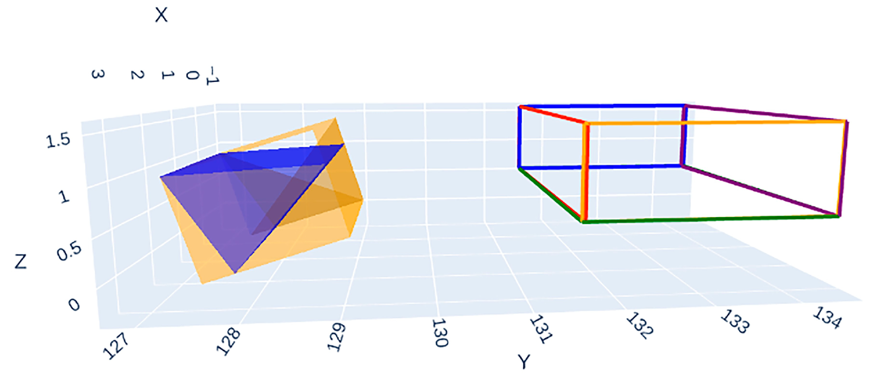
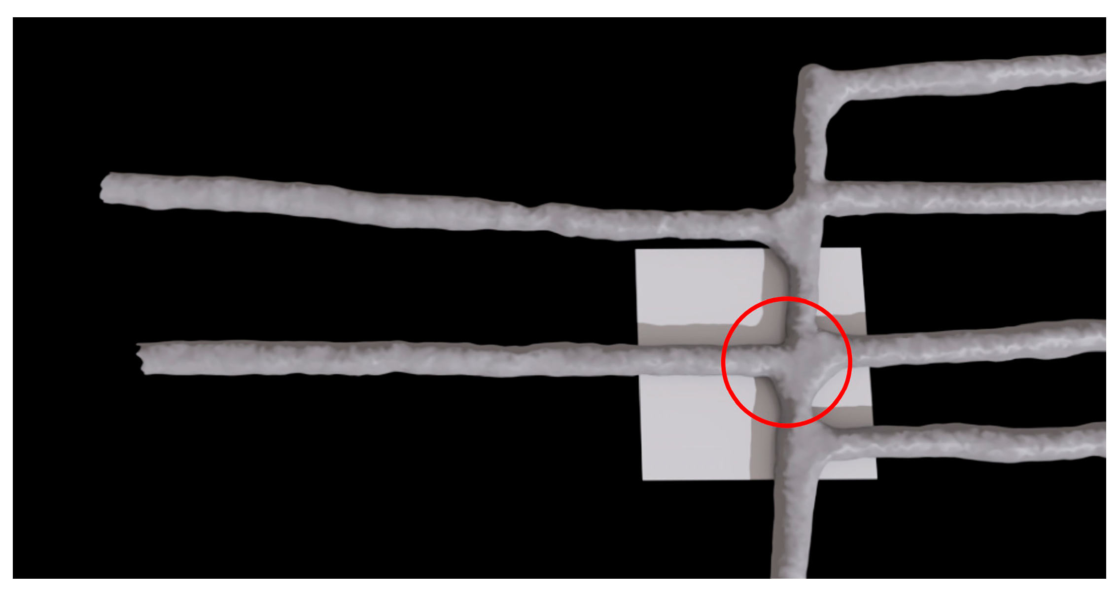
2.3.3. Constructing the OBB

The OBB is the minimum-volume rectangular prism that tightly encloses an object or a point cloud. Unlike an AABB, an OBB’s orientation is aligned with the principal axes of the enclosed object rather than being constrained to the world coordinate axes. This tighter fit reduces the enclosed volume, thereby enhancing the precision and efficiency of subsequent collision detection algorithms [54].

The construction of the OBB follows these steps:

1.

Compute the principal direction of the point cloud: The first step in constructing an OBB is determining the primary direction of the point cloud. This is typically achieved using principal component analysis (PCA), which identifies the principal directions by analyzing the covariance matrix of the point cloud. The principal direction corresponds to the direction with the highest variance in the data;

2.

Steps of PCA: Compute the mean of the point cloud:

$$\mu ={\displaystyle \frac{1}{N}}{\displaystyle \sum }_{i=1}^N{x}_i.$$

(22)

where $x_i$ represents the $i$-th point in the point cloud, and $\mu$ is the mean of all points.

Compute the covariance matrix of the point cloud:

$$\sum ={\displaystyle \frac{1}{N}}{\displaystyle \sum }_{i=1}^N(x_i-\mu ){(x_i-\mu )}^T$$

(23)

Performing eigenvalue decomposition yields the eigenvectors and eigenvalues of the covariance matrix. The eigenvectors represent the principal directions, while the eigenvalues indicate the variance along each direction;

3.

Rotating the point cloud: Using the principal direction obtained from PCA, a rotation matrix is constructed so that after the point cloud is projected into the new coordinate system, the principal direction aligns with the coordinate axes;

4.

Calculating the dimensions of the point cloud: After rotation, the point cloud typically forms a rectangular box along three axes. The dimensions (length, width, and height) of the bounding box can be determined by calculating the maximum and minimum values of the rotated point cloud along each axis.

Assumptions of the projections of the rotated point cloud on the X, Y, and Z are as follows:

$$\begin{array}{l}mi{n}_x=\min \left(x_{rot}\right), ma{x}_x=\max \left(x_{rot}\right)\\ mi{n}_y=\min \left(y_{rot}\right) , ma{x}_y=\max \left(y_{rot}\right)\\ mi{n}_z=\min \left(z_{rot}\right), ma{x}_z=\max \left(z_{rot}\right)\end{array}$$

(24)

The $length$, $width$, and $height$ of the bounding box are as follows:

$$\begin{array}{l}length=ma{x}_x-mi{n}_x\\ width=ma{x}_y-mi{n}_y\\ height=ma{x}_z-mi{n}_z\end{array}$$

(25)

5.

Determine the center point and rotation information of the bounding box: The center ($c$) of the OBB is the mean of the rotated point cloud:

$$c=\mu$$

(26)

The rotation information is provided by the rotation matrix calculated through PCA, which represents the rotation of the bounding box relative to the world coordinate system.

The PCA-based method described above is standard for constructing an OBB from a general, dense point cloud. However, in our specific application, the structures of the bucket and truck are well-defined and geometrically simple. Therefore, instead of using a full point cloud, we simplify the process by extracting a small set of key points (e.g., the six vertices of the bucket). The OBB is then constructed directly from these key points using geometric principles analogous to those in PCA.

The OBB for the bucket is constructed from the set of its six previously computed key points. Similarly, an OBB for the mining truck could be constructed from the vertices of its cargo bed. However, as the truck’s cargo bed is an open, concave container (effectively a rectangular prism missing its top face), a single OBB would poorly represent its geometry. A single OBB is not applicable, as it would enclose a large empty volume above the cargo bed, leading to inaccurate collision detection (i.e., false positives). To address this issue, our approach models the truck’s cargo bed as a composite of its five constituent planar surfaces. A distinct OBB is then constructed for each of these five faces. A visualization of the resulting OBBs for both the bucket and the truck is provided in Figure 12.

2.3.4. SAT Method for Collision Detection

The SAT is a geometric algorithm for determining whether two convex polyhedra are intersecting. The core principle of SAT states that two convex objects do not intersect if and only if there exists a “separating axis” onto which the projections of the two objects do not overlap. Conversely, if the objects’ projections overlap on all potential separating axes, the objects are deemed to be intersecting [54].

The basic process of the SAT algorithm can be divided into the following steps:

1.

Generation of candidate separating axes:

For two 3D objects, the normal directions of each surface are first extracted as the primary separating axes. Next, the perpendicular direction of the direction vectors of each pair of edges between the two objects is calculated (using the cross product), and these directions are added to the set of candidate axes. Finally, all axes are merged and duplicates are removed to form a complete list of separating axes to be tested;

2.

Projection onto separating axes:

For each separating axis, the projection of both objects onto the axis is computed. If the projections of the two objects overlap, they are not separated along that axis; if the projections do not overlap on any axis, the objects are not colliding. For each object, the minimum and maximum values of its projection on the separating axis are calculated, resulting in a projection interval. These intervals are then compared to check if they overlap;

3.

Collision determination:

If the projection intervals of the two objects do not overlap on any separating axis, the objects are considered not to collide. If the projection intervals of the two objects overlap on all separating axes, it indicates that a collision has occurred.

In conclusion, during the ore loading process from the LHD to the mining truck, the bucket may collide with the mining truck. Based on the pose of key points, OBBs for both the bucket and the mining truck are constructed, and the SAT method is used to detect whether the bucket’s OBB collides with the OBB of the mining truck.

3. Results

In this study, a simulated underground metal mining environment was constructed using the Isaac Sim simulation platform. The environment includes tunnels, an LHD machine, and a mining truck. A series of experiments were conducted within this simulation environment to verify the feasibility of the proposed collision detection algorithm.

3.1. Experimental Setup

The experiments were performed on the Isaac Sim platform, running on a workstation with an Intel Core i7-10700K CPU (Intel Corporation, Santa Clara, CA, USA), an NVIDIA GeForce RTX 2060 SUPER GPU (NVIDIA Corporation, Santa Clara, CA, USA), and Ubuntu 20.04. The simulated environment features a tunnel, an LHD machine, and a mining truck.

• Algorithm 1 (LiDAR-based) Parameters:
  • LiDAR Sensor: 120° horizontal FoV, 60° vertical FoV.
  • Voxel Downsampling: Voxel size = 0.1 m.
  • DBSCAN: Neighborhood radius ($\epsilon$) = 0.11 m, minimum points ($minPts$) = 4. These parameters were empirically tuned to balance sensitivity and noise rejection.
  • Collision Threshold: 0.15 m. An alarm is triggered if the minimum distance between the bucket and tunnel point clouds is less than this value.

2.

Algorithm 2 (Kinematics-based) Parameters:

• Sensor Model: The inclination sensors were simulated to provide ideal, noise-free measurements. This approach was chosen to validate the intrinsic accuracy of the kinematic model itself.
• Evaluation Metric: The SAT output. A negative overlap value indicates a collision (penetration), with its magnitude representing the penetration depth. A positive value indicates separation, with its magnitude representing the minimum clearance distance between the OBBs.

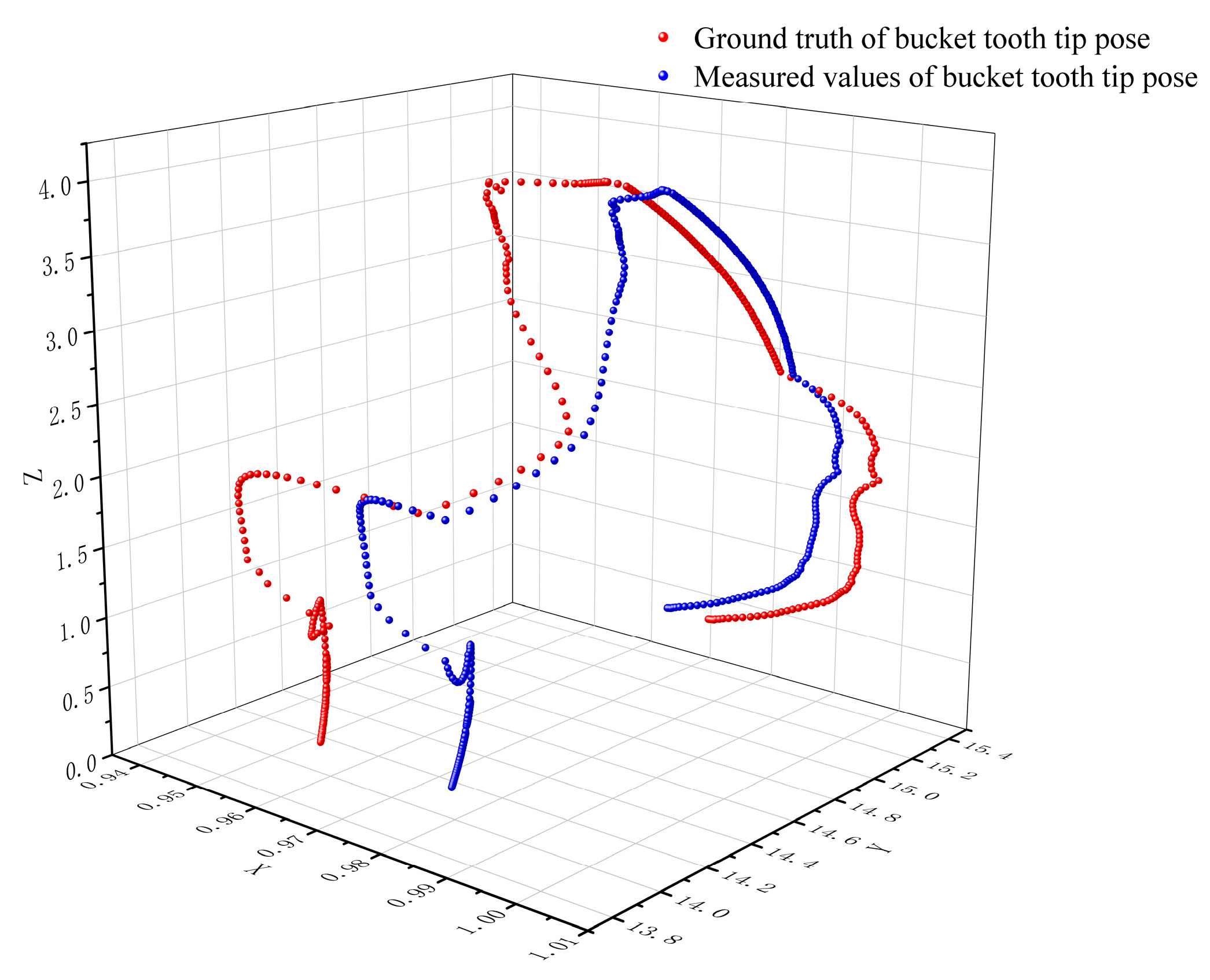
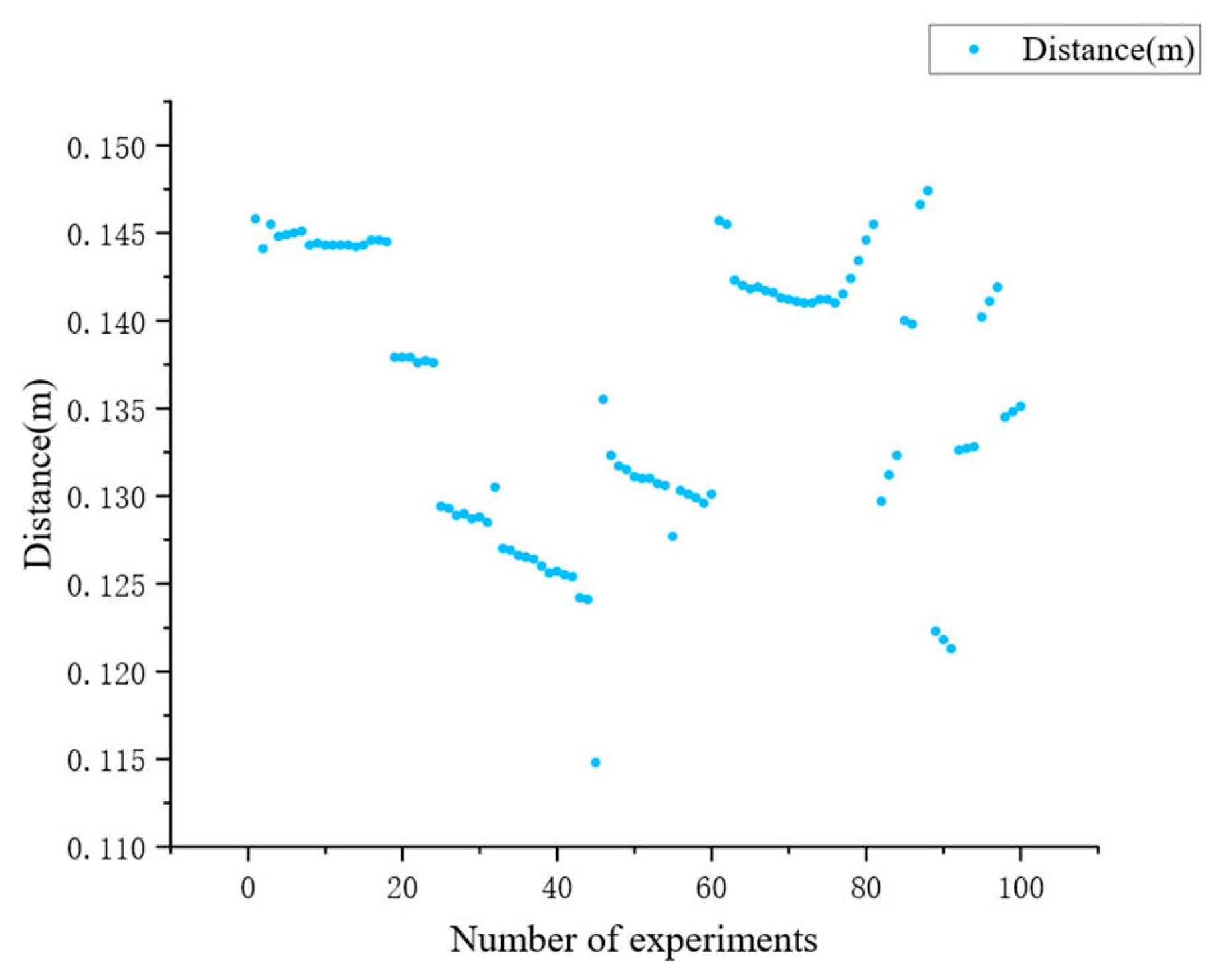
3.2. Verification of the Bucket Tooth Tip Pose

To verify the accuracy of the bucket tooth tip pose formula, experiments were conducted within the simulation environment. First, the LHD machine’s boom was raised to its maximum height within the tunnel. Then, the bucket was controlled to rotate downward to its maximum angle. During this process, both the ground truth and measured values of the bucket tooth tip pose were recorded for subsequent calculation and analysis. A total of 493 ground truth and 493 measured pose values were obtained. These values were rounded to four decimal places, and their distribution in 3D space is shown in Figure 13.

This paper evaluates the proximity between the ground truth and measured values of the bucket tooth tip pose by calculating the Euclidean distance between them. The calculation results are shown in

Table 2. Pose error of the bucket tooth tip, including the maximum, minimum, and average distances.

Maximum Distance (m)	Minimum Distance (m)	Average Distance (m)
0.0252	0	0.0141

.

From the calculation results, it is observed that the maximum distance between the ground truth and measured values is 0.0252 m. Considering the large size of the LHD, this distance falls within a reasonable range. The minimum distance is 0 m, as the sensor measurements in the simulation environment are highly accurate, allowing for the possibility of a zero distance. The average distance is 0.0141 m, indicating that throughout the entire ore loading process, the pose error remains relatively stable. This low error margin is crucial, as it confirms that the kinematic model is a highly reliable foundation for the subsequent OBB construction and collision detection. The high accuracy validates that our method of using inclination sensors and geometric calculations can effectively and precisely track the bucket’s pose, even when external sensors like LiDAR are occluded. This lays a solid foundation for the reliability of the kinematics-based collision detection algorithm.

3.3. Validation of Collision Detection Algorithm in Different Scenarios

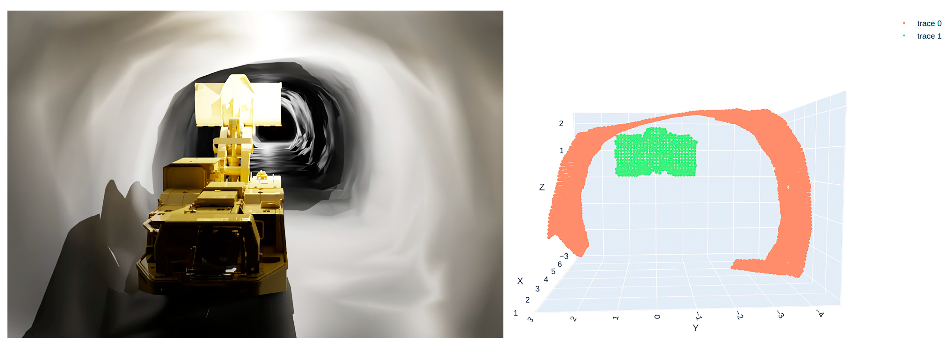
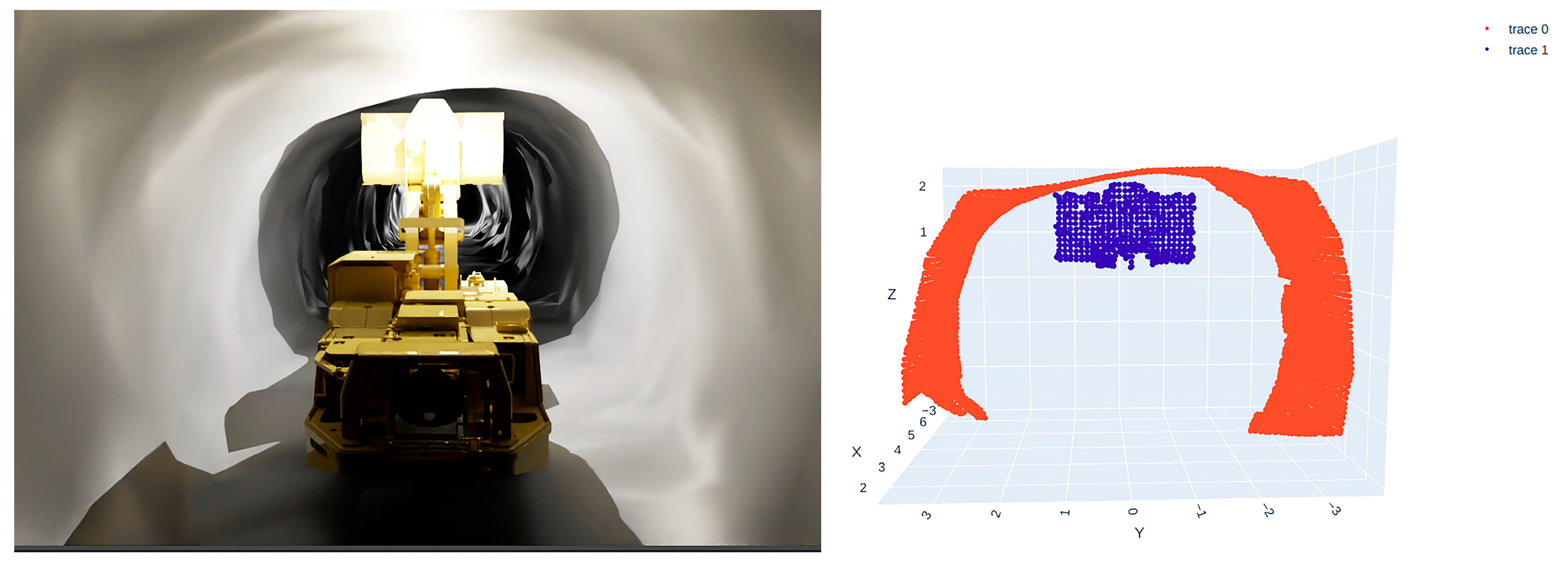
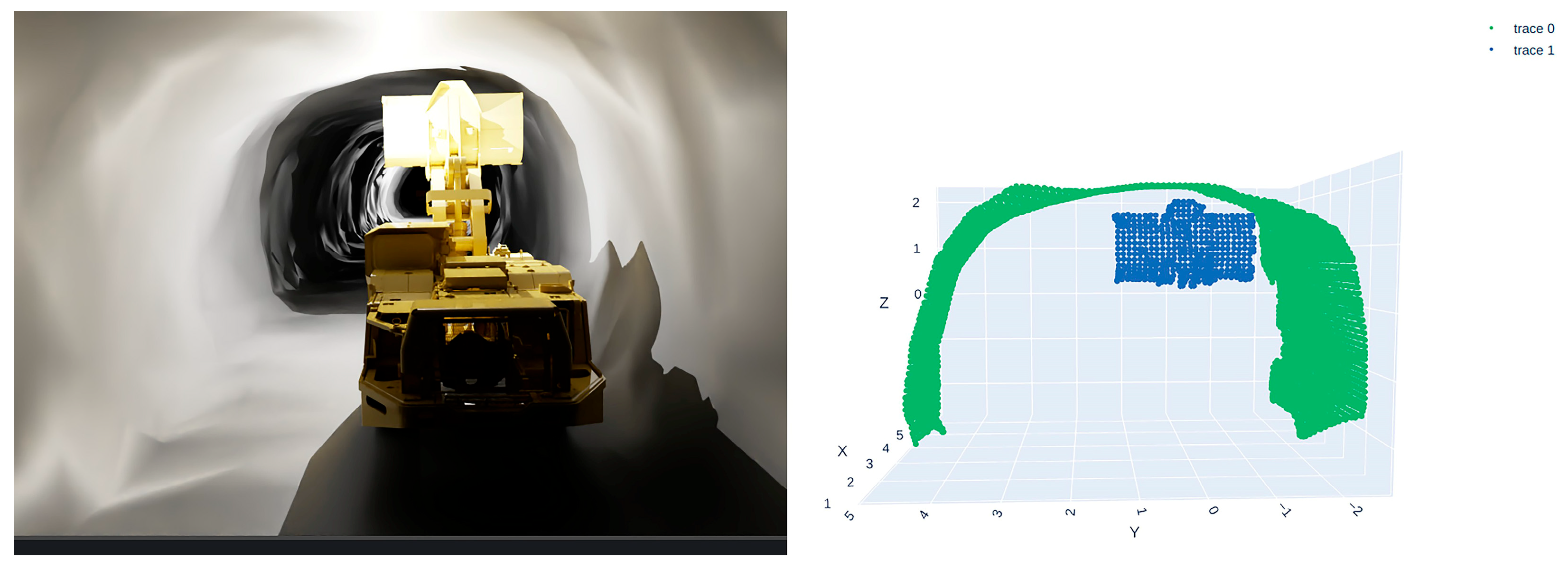
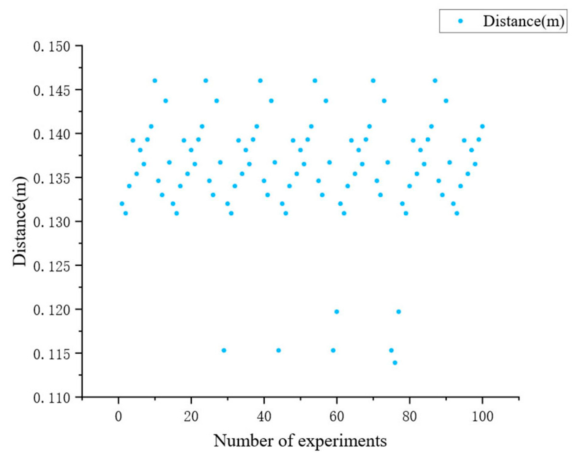
3.3.1. Validation of Bucket and Tunnel Wall Collision Detection Algorithm

During the upward lifting process of the LHD’s boom, there is a potential for the bucket to collide with the tunnel wall. Since the tunnel wall is arch-shaped, this study performed 100 lifting actions of the LHD’s boom on the left (Figure 14), middle (Figure 15), and right (Figure 16) sides of the tunnel to verify the effectiveness of the collision detection algorithm.

To test the effectiveness and reliability of the LiDAR-based algorithm (Section 2.2) in preventing collisions between the bucket and the tunnel wall, three challenging scenarios were designed to simulate common operational risks. In each scenario, the LHD attempts to lift its boom 100 times.

• Scenario 1: LHD positioned close to the left tunnel wall (Figure 14);
• Scenario 2: LHD positioned in the center of the tunnel (Figure 15);
• Scenario 3: LHD positioned close to the right tunnel wall (Figure 16).

When the system detects a collision between the bucket and the tunnel wall, the distance between the two is recorded, as shown in the figures below.

The performance of the algorithm was rigorously validated through 300 trials, achieving a perfect 100% detection rate with no instances of false alarms or missed detections, establishing its exceptional reliability. A deeper analysis of the results, presented in Figure 17, Figure 18 and Figure 19 reveals a critical insight: alarms were consistently triggered when the minimum distance was just shy of the 0.15 m threshold. This outcome has two profound implications for the system’s effectiveness. Firstly, it validates that the 0.15 m threshold is not merely a random value but a well-calibrated parameter that provides a timely and practical safety margin. Secondly, and more critically, it underscores the power of the DBSCAN clustering algorithm. The ability to maintain the integrity of two distinct point cloud clusters when they are nearly in contact is a non-trivial challenge. The algorithm’s success here proves that DBSCAN effectively prevents cluster merging, a common failure mode that would lead to a catastrophic missed detection. Therefore, the synergistic effect of a precise threshold and a robust clustering method confirms the validity and superiority of our proposed approach.

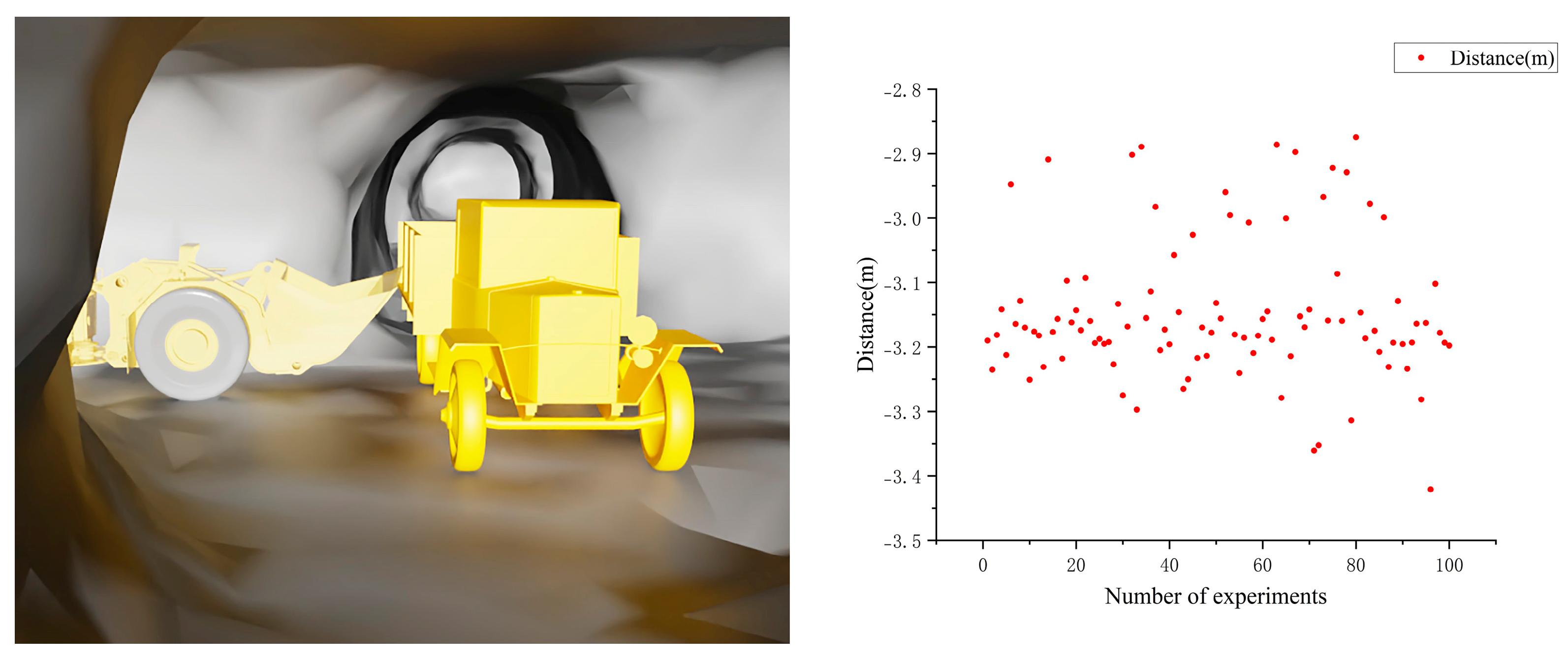
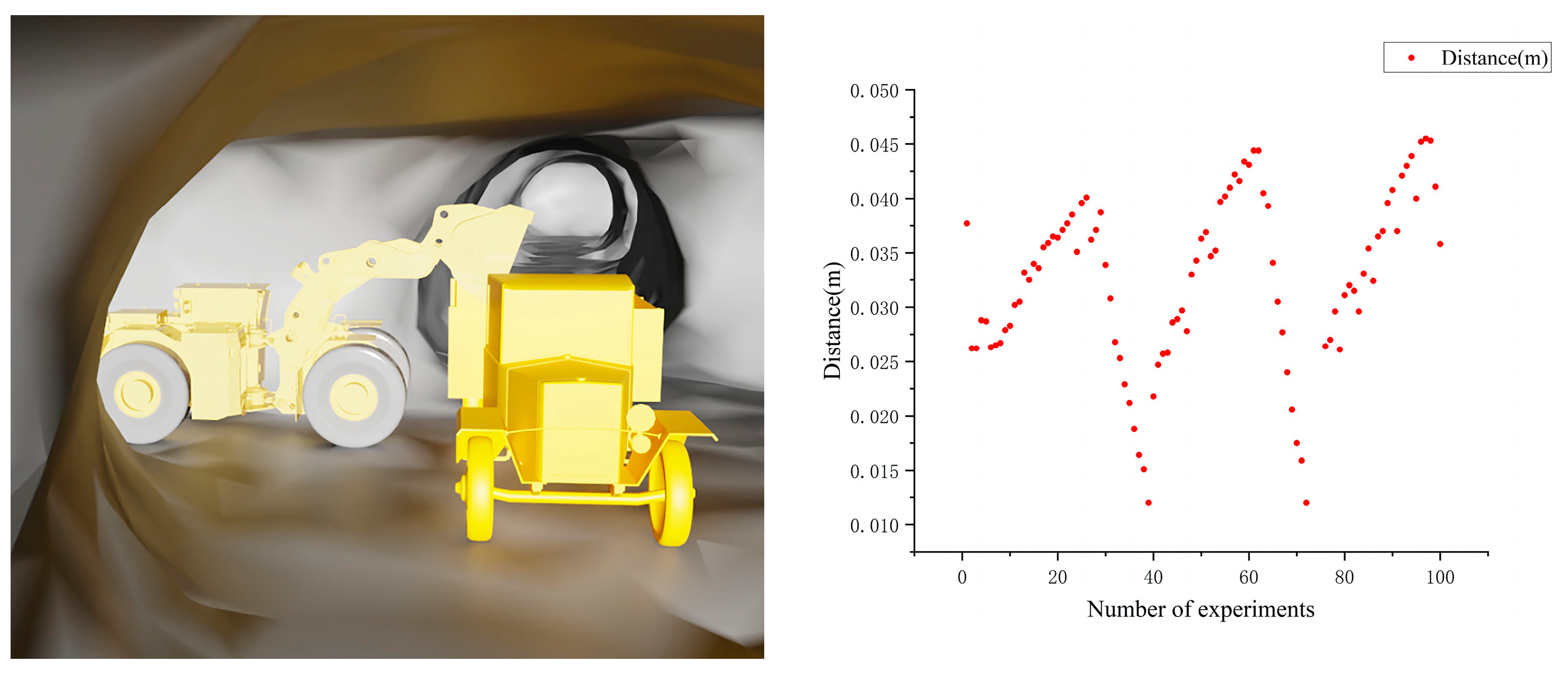
3.3.2. Verification of the Collision Detection Algorithm for the Bucket and Mining Truck

To verify the feasibility of the collision detection algorithm between the bucket and the mining truck, three distinct operational scenarios were tested, with each scenario repeated 100 times. During the experiments, the collision detection results and the distances between the separating axes were recorded. Specifically, after traversing all separating axes, the overlap on each axis was calculated. If there was any axis with no overlap, the smallest positive overlap among all axes was recorded. If all axes had overlap, the largest negative overlap was recorded. The experimental location is shown in Figure 20.

First, without lifting the boom, the LHD approaches the mining truck at varying speeds. This experiment was repeated 100 times, and the results, as shown in Figure 21, demonstrate that collisions were successfully detected in each instance, as expected. The range of the maximum negative overlap during each collision was (−3.4209 m, −2.8743 m).

Next, a series of operations in the simulated ore loading process were conducted, including the LHD dumping ore into the mining truck. This experiment was repeated 100 times, and the results, as shown in Figure 22, demonstrate that no collision was detected when the bucket entered the mining truck’s compartment, as expected, since the truck’s compartment is not a completely enclosed space. The range of the minimum positive overlap during non-collision events was (0.0120 m, 0.0455 m).

The LHD’s position was moved directly above the edge of the mining truck. If ore loading operations were performed at this position, a collision would inevitably occur when the LHD dumped the ore. This experiment was repeated 100 times, and the results, as shown in Figure 23, demonstrate that a collision was detected every time, as expected. The range of the maximum negative overlap during each collision was (−1.5760 m, −1.2952 m).

The results show a perfect 100% success rate in correctly identifying the outcome for all 300 trials. The SAT output provides unambiguous results. In collision scenarios (1 and 3), the system consistently reported a negative overlap (Figure 21 and Figure 23), confirming penetration. The magnitude of this value can even serve as an indicator of the potential severity of the collision. The success of Scenario 2 is particularly significant. The algorithm correctly registered no collision, reporting a small but safe positive separation distance (Figure 22). This directly validates our design choice to model the open truck bed as five individual planar OBBs. A naive single-OBB approach would have enclosed the empty space above the cargo bed, leading to constant false alarms during this critical, normal operational phase. Our method completely avoids this pitfall. The algorithm’s ability to differentiate between the safe clearance in Scenario 2 and the definite collision in Scenario 3, which can be geometrically very similar, showcases the high precision of the SAT method when applied to accurately constructed OBBs.

In conclusion, the comprehensive experimental results provide compelling quantitative validation for the two proposed collision detection algorithms. We have demonstrated that

• The kinematic pose formula achieves centimeter-level accuracy (1.41 cm average error), establishing a reliable foundation for the subsequent collision detection;
• The algorithm for bucket-and-tunnel collision detection, which is based on LiDAR, provides 100% reliable, real-time protection. Its robustness is underscored by the DBSCAN method’s success in preventing cluster-merging failures, even when the objects are in extreme proximity;
• The kinematics-based algorithm for bucket-and-truck collision detection also achieved a perfect 100% success rate, critically overcoming the challenges of sensor occlusion and solving the intractable false-alarm problem inherent in naive models of the open-top truck.

By synergistically combining these two complementary algorithms, this study delivers a holistic safety solution that provides comprehensive coverage for the entire ore loading process in challenging underground environments.

4. Discussion

The findings of this study confirm that the proposed dual-algorithm system provides a robust and reliable solution for collision detection in LHD loading operations. The successful validation of the kinematic model with centimeter-level accuracy is not merely a confirmation of the DH parameters but rather establishes the viability of a model-based approach as a powerful fallback for when direct-sensing methods, like LiDAR, are compromised by occlusion—a frequent occurrence in confined underground environments.

In the context of previous studies, much of the existing work on kinematic modeling has focused on equipment like excavators in open-pit mines or construction sites. Our research extends this paradigm to the unique challenges of underground mining, specifically addressing the critical failure point of sensor occlusion during the bucket–truck interaction. Furthermore, our solution for the truck collision problem represents a significant advancement. While OBBs and SAT are established techniques, our key innovation lies in the multi-faceted OBB representation of the truck bed. This novel approach effectively resolves the persistent issue of false-positive alarms that plagues naive, single-volume models, demonstrating a practical path toward system reliability that previous approaches have not addressed.

The broader implications of this work are twofold. From a practical safety perspective, this system offers a tangible pathway to reducing equipment damage, operational downtime, and, most importantly, human-involved accidents in one of the most hazardous phases of underground mining. It represents a critical enabling technology for higher levels of automation. From a technological standpoint, our work underscores the power of a synergistic, complementary system design. By combining a perception-based algorithm (LiDAR) for general awareness with a model-based algorithm (kinematics) for precision tasks under occlusion, we showcase a robust architectural pattern applicable to a wide range of autonomous robotic systems operating in complex, unstructured environments.

However, we must acknowledge the limitations of this study, which in turn highlight promising directions for future research. A primary limitation is the reliance on an ideal, noise-free sensor model in the simulation. Future work should incorporate stochastic sensor models to rigorously evaluate the system’s robustness and explore the integration of state estimation filters (e.g., Kalman filters) to handle real-world data imperfections. Secondly, this validation was conducted entirely within a simulation. The ultimate test will be the deployment and verification of this system on a physical LHD platform in a real-world mining environment. Finally, our current work focuses on static obstacles (tunnel and parked truck); extending the system to detect and react to dynamic obstacles, such as other vehicles or personnel, remains a critical next step towards a fully comprehensive safety solution.

5. Conclusions

In response to the complex environment of underground metal mines and the unmanned ore loading process, we developed a collision detection algorithm tailored to this context. The algorithm employs laser radar to address the challenges of the underground environment, and it incorporates a series of preprocessing steps such as point cloud filtering, downsampling, clustering, and segmentation. Collision detection is then performed based on a KD-tree structure with appropriately set thresholds. To address the issue of sensor occlusion, we derived a calculation formula for the bucket tooth pose. Using the geometric features of the bucket, we calculated the pose of key points on the bucket and established bounding boxes, which were subsequently used for collision detection via the SAT. Experimental results show that our pose calculation formula is applicable to the entire ore loading process, providing accurate results. The collision detection algorithms for both the bucket–tunnel wall and the bucket–mining truck are equally effective and function well in the underground metal mining environment.

References

1. Li, J.; Zhan, K. Intelligent Mining Technology for an Underground Metal Mine Based on Unmanned Equipment. Engineering 2018, 4, 381–391. [Google Scholar] [CrossRef]
2. Cucuzza, J. The Status and Future of Mining Automation: An Overview. IEEE Ind. Electron. Mag. 2021, 15, 6–12. [Google Scholar] [CrossRef]
3. Wang, J.; Wang, L.; Peng, P.; Jiang, Y.; Wu, J.; Liu, Y. Efficient and Accurate Mapping Method of Underground Metal Mines Using Mobile Mining Equipment and Solid-State Lidar. Measurement 2023, 221, 113581. [Google Scholar] [CrossRef]
4. Wang, J.; Wang, L.; Jiang, Y.; Peng, P.; Wu, J.; Liu, Y. A Novel Global Re-Localization Method for Underground Mining Vehicles in Haulage Roadways: A Case Study of Solid-State LiDAR-Equipped Load-Haul-Dump Vehicles. Tunn. Undergr. Space Technol. 2025, 156, 106270. [Google Scholar] [CrossRef]
5. Xiao, W.; Liu, M.; Chen, X. Research Status and Development Trend of Underground Intelligent Load-Haul-Dump Vehicle—A Comprehensive Review. Appl. Sci. 2022, 12, 9290. [Google Scholar] [CrossRef]
6. Huh, S.; Lee, U.; Shim, H.; Park, J.-B.; Noh, J.-H. Development of an Unmanned Coal Mining Robot and a Tele-Operation System. In Proceedings of the 2011 11th International Conference on Control, Automation and Systems, Gyeonggi-do, Republic of Korea, 26–29 October 2011; IEEE: Piscataway, NJ, USA, 2011; pp. 31–35. [Google Scholar]
7. Ranjan, A.; Zhao, Y.; Sahu, H.B.; Misra, P. Opportunities and Challenges in Health Sensing for Extreme Industrial Environment: Perspectives from Underground Mines. IEEE Access 2019, 7, 139181–139195. [Google Scholar] [CrossRef]
8. Maric, B.; Jurican, F.; Orsag, M.; Kovacic, Z. Vision Based Collision Detection for a Safe Collaborative Industrial Manipulator. In Proceedings of the 2021 IEEE International Conference on Intelligence and Safety for Robotics (ISR), Tokoname, Japan, 4–6 March 2021; IEEE: Piscataway, NJ, USA, 2021; pp. 334–337. [Google Scholar]
9. Bauer, P.; Hiba, A. Vision Only Collision Detection with Omnidirectional Multi-Camera System. IFAC-Pap. 2017, 50, 15215–15220. [Google Scholar] [CrossRef]
10. Zhang, F.; Liu, H.; Chen, Z.; Wang, L.; Zhang, Q.; Guo, L. Collision Risk Warning Model for Construction Vehicles Based on YOLO and DeepSORT Algorithms. J. Constr. Eng. Manag. 2024, 150, 04024053. [Google Scholar] [CrossRef]
11. Lu, S.; Xu, Z.; Wang, B. Human-Robot Collision Detection Based on the Improved Camshift Algorithm and Bounding Box. Int. J. Control Autom. Syst. 2022, 20, 3347–3360. [Google Scholar] [CrossRef]
12. Imam, M.; Baina, K.; Tabii, Y.; Ressami, E.M.; Adlaoui, Y.; Benzakour, I.; Abdelwahed, E.H. The Future of Mine Safety: A Comprehensive Review of Anti-Collision Systems Based on Computer Vision in Underground Mines. Sensors 2023, 23, 4294. [Google Scholar] [CrossRef] [PubMed]
13. Xiang, Q.; Chen, C.; Jiang, Y. Servo Collision Detection Control System Based on Robot Dynamics. Sensors 2025, 25, 1131. [Google Scholar] [CrossRef] [PubMed]
14. Sun, S.; Song, C.; Wang, B.; Huang, H. Research on Dynamic Parameter Identification and Collision Detection Method for Cooperative Robots. Ind. Robot. 2023, 50, 1024–1035. [Google Scholar] [CrossRef]
15. Xu, T.; Fan, J.; Fang, Q.; Zhu, Y.; Zhao, J. A New Robot Collision Detection Method: A Modified Nonlinear Disturbance Observer Based-on Neural Networks. J. Intell. Fuzzy Syst. 2020, 38, 175–186. [Google Scholar] [CrossRef]
16. Ye, J.; Fan, Y.; Kang, Q.; Liu, X.; Wu, H.; Zheng, G. MomentumNet-CD: Real-Time Collision Detection for Industrial Robots Based on Momentum Observer with Optimized BP Neural Network. Machines 2025, 13, 334. [Google Scholar] [CrossRef]
17. Zhang, T.; Hong, J. Collision Detection Method for Industrial Robot Based on Envelope-like Lines. Ind. Robot. 2019, 46, 510–517. [Google Scholar] [CrossRef]
18. Zhang, T.; Ge, P.; Zou, Y.; He, Y. Robot Collision Detection Without External Sensors Based on Time-Series Analysis. J. Dyn. Syst. Meas. Control 2021, 143, 041005. [Google Scholar] [CrossRef]
19. Zhang, D.; Zhao, J.; Zhang, H. Six-Degree-of-Freedom Manipulator Fast Collision Detection Algorithm Based on Sphere Bounding Box. In Proceedings of the 2024 2nd International Conference on Artificial Intelligence and Automation Control (AIAC), Guangzhou, China, 20–22 December 2024; IEEE: Piscataway, NJ, USA, 2024; pp. 184–187. [Google Scholar]
20. Dong, L.; Xiao, Y.; Li, Y.; Shi, R. A Collision Detection Algorithm Based on Sphere and EBB Mixed Hierarchical Bounding Boxes. IEEE Access 2024, 12, 62719–62729. [Google Scholar] [CrossRef]
21. Nie, S.; Chen, B.; Li, Y.; Wang, D.; Xu, Y. The Autonomous Route Planning Algorithm for Rock Drilling Manipulator Based on Collision Detection. J. Field Robot. 2025, in press. [CrossRef]
22. Yang, W.; Ji, Y.; Zhang, X.; Zhao, D.; Ren, Z.; Wang, Z.; Tian, S.; Du, Y.; Zhu, L.; Jiang, J. A Multi-Camera System-Based Relative Pose Estimation and Virtual-Physical Collision Detection Methods for the Underground Anchor Digging Equipment. Mathematics 2025, 13, 559. [Google Scholar] [CrossRef]
23. Hou, D.; Wang, X.; Liu, J.; Yang, B.; Hou, G. Research on Collision Avoidance Technology of Manipulator Based on AABB Hierarchical Bounding Box Algorithm. In Proceedings of the 2021 5th Asian Conference on Artificial Intelligence Technology (ACAIT), Haikou, China, 29–31 October 2021; IEEE: Piscataway, NJ, USA, 2021; pp. 406–409. [Google Scholar]
24. Gan, B.; Dong, Q. An Improved Optimal Algorithm for Collision Detection of Hybrid Hierarchical Bounding Box. Evol. Intel. 2022, 15, 2515–2527. [Google Scholar] [CrossRef]
25. Schauer, J.; Nüchter, A. Collision Detection between Point Clouds Using an Efficient K-d Tree Implementation. Adv. Eng. Inform. 2015, 29, 440–458. [Google Scholar] [CrossRef]
26. Huang, Z.; Yang, X.; Min, J.; Wang, H.; Wei, P. Collision Detection Algorithm on Abrasive Belt Grinding Blisk Based on Improved Octree Segmentation. Int. J. Adv. Manuf. Technol. 2022, 118, 4105–4121. [Google Scholar] [CrossRef]
27. Lu, B.; Wang, Q.; Li, A. Massive Point Cloud Space Management Method Based on Octree-Like Encoding. Arab. J. Sci. Eng. 2019, 44, 9397–9411. [Google Scholar] [CrossRef]
28. Xiaolong, C.; Zhangyan, C.; Jun, X.; Long, Z.; Ying, W. Voxel-Based Meshing Collision Detection Accelerating Algorithm for DDA2D. J. Univ. Chin. Acad. Sci. 2023, 40, 540. [Google Scholar]
29. Yang, P.; Shen, F.; Xu, D.; Liu, R. A Fast Collision Detection Method Based on Point Clouds and Stretched Primitives for Manipulator Obstacle-Avoidance Motion Planning. Int. J. Adv. Robot. Syst. 2024, 21, 17298806241283382. [Google Scholar] [CrossRef]
30. Wang, Z.; Yu, B.; Chen, J.; Liu, C.; Zhan, K.; Sui, X.; Xue, Y.; Li, J. Research on Lidar Point Cloud Segmentation and Collision Detection Algorithm. In Proceedings of the 2019 6th International Conference on Information Science and Control Engineering (ICISCE), Shanghai, China, 20–22 December 2019; IEEE: Piscataway, NJ, USA, 2019; pp. 475–479. [Google Scholar]
31. Yang, A.; Liu, Q.; Naeem, W.; Fei, M. Robot Dynamic Collision Detection Method Based on Obstacle Point Cloud Envelope Model. In Intelligent Equipment, Robots, and Vehicles; Han, Q., McLoone, S., Peng, C., Zhang, B., Eds.; Springer: Singapore, 2021; Volume 1469, pp. 370–378. [Google Scholar]
32. Niwa, T.; Masuda, H. Interactive Collision Detection for Engineering Plants Based on Large-Scale Point-Clouds. Comput.-Aided Des. Appl. 2016, 13, 511–518. [Google Scholar] [CrossRef]
33. Ueki, S.; Mouri, T.; Kawasaki, H. Collision Avoidance Method for Hand-Arm Robot Using Both Structural Model and 3D Point Cloud. In Proceedings of the 2015 IEEE/SICE International Symposium on System Integration (SII), Nagoya, Japan, 12–13 December 2015; IEEE: Piscataway, NJ, USA, 2015; pp. 193–198. [Google Scholar]
34. Ramsey, C.W.; Kingston, Z.; Thomason, W.; Kavraki, L.E. Collision-Affording Point Trees: SIMD-Amenable Nearest Neighbors for Fast Collision Checking. arXiv 2024, arXiv:2406.02807. [Google Scholar]
35. López-Adeva Fernández-Layos, P.; Merchante, L.F.S. Convex Body Collision Detection Using the Signed Distance Function. Comput. Aided Des. 2024, 170, 103685. [Google Scholar] [CrossRef]
36. Xia, R.; Wang, D.; Mou, C. Collision Detection Between Convex Objects Using Pseudodistance and Unconstrained Optimization. IEEE Trans. Robot. 2025, 41, 253–268. [Google Scholar] [CrossRef]
37. Heo, Y.J.; Kim, D.; Lee, W.; Kim, H.; Park, J.; Chung, W.K. Collision Detection for Industrial Collaborative Robots: A Deep Learning Approach. IEEE Robot. Autom. Lett. 2019, 4, 740–746. [Google Scholar] [CrossRef]
38. Wu, D.; Yu, Z.; Adili, A.; Zhao, F. A Self-Collision Detection Algorithm of a Dual-Manipulator System Based on GJK and Deep Learning. Sensors 2023, 23, 523. [Google Scholar] [CrossRef] [PubMed]
39. Cao, J.; Wang, M. A Fast and Generalized Broad-Phase Collision Detection Method Based on KD-Tree Spatial Subdivision and Sweep-and-Prune. IEEE Access 2023, 11, 44696–44710. [Google Scholar] [CrossRef]
40. Qi, B.; Pang, M. An Enhanced Sweep and Prune Algorithm for Multi-Body Continuous Collision Detection. Vis. Comput. 2019, 35, 1503–1515. [Google Scholar] [CrossRef]
41. Li, J.-R.; Xin, R.-H.; Wang, Q.-H.; Li, Y.-F.; Xie, H.-L. Graphic-Enhanced Collision Detection for Robotic Manufacturing Applications in Complex Environments. Int. J. Adv. Manuf. Technol. 2024, 130, 3291–3305. [Google Scholar] [CrossRef]
42. Serpa, Y.R.; Rodrigues, M.A.F. Flexible Use of Temporal and Spatial Reasoning for Fast and Scalable CPU Broad-Phase Collision Detection Using KD-Trees. Comput. Graph. Forum 2019, 38, 260–273. [Google Scholar] [CrossRef]
43. Chitalu, F.M.; Dubach, C.; Komura, T. Binary Ostensibly-Implicit Trees for Fast Collision Detection. Comput. Graph. Forum 2020, 39, 509–521. [Google Scholar] [CrossRef]
44. Pinkham, R.; Zeng, S.; Zhang, Z. QuickNN: Memory and Performance Optimization of k-d Tree Based Nearest Neighbor Search for 3D Point Clouds. In Proceedings of the 2020 IEEE International Symposium on High Performance Computer Architecture (HPCA), San Diego, CA, USA, 22–26 February 2020; IEEE: Piscataway, NJ, USA, 2020; pp. 180–192. [Google Scholar]
45. Park, J.S.; Park, C.; Manocha, D. Efficient Probabilistic Collision Detection for Non-Convex Shapes. In Proceedings of the 2017 IEEE International Conference on Robotics and Automation (ICRA), Singapore, 29 May–3 June 2017; IEEE: Piscataway, NJ, USA, 2017; pp. 1944–1951. [Google Scholar]
46. Zou, Y.; Zhang, H.; Feng, D.; Liu, H.; Zhong, G. Fast Collision Detection for Small Unmanned Aircraft Systems in Urban Airspace. IEEE Access 2021, 9, 16630–16641. [Google Scholar] [CrossRef]
47. Fan, Q.; Tao, B.; Gong, Z.; Zhao, X.; Ding, H. Fast Global Collision Detection Method Based on Feature-Point-Set for Robotic Machining of Large Complex Components. IEEE Trans. Autom. Sci. Eng. 2023, 20, 470–481. [Google Scholar] [CrossRef]
48. Montaut, L.; Le Lidec, Q.; Petrik, V.; Sivic, J.; Carpentier, J. GJK++: Leveraging Acceleration Methods for Faster Collision Detection. IEEE Trans. Robot. 2024, 40, 2564–2581. [Google Scholar] [CrossRef]
49. Melero, F.J.; Aguilera, Á.; Feito, F.R. Fast Collision Detection between High Resolution Polygonal Models. Comput. Graph. 2019, 83, 97–106. [Google Scholar] [CrossRef]
50. Liu, Z.; Yan, S.; Zou, K.; Xie, M. Collision Detection Method for Anchor Digging Machine Water Drilling Rig. Sci. Rep. 2025, 15, 726. [Google Scholar] [CrossRef] [PubMed]
51. Ren, T.; Dong, Y.; Wu, D.; Chen, K. Collision Detection and Identification for Robot Manipulators Based on Extended State Observer. Control Eng. Pract. 2018, 79, 144–153. [Google Scholar] [CrossRef]
52. Ester, M.; Kriegel, H.-P.; Sander, J.; Xu, X. A Density-Based Algorithm for Discovering Clusters in Large Spatial Databases with Noise. In Proceedings of the Second International Conference on Knowledge Discovery and Data Mining, Portland, OR, USA, 2–4 August 1996; AAAI Press: Washington, DC, USA, 1996; pp. 226–231. [Google Scholar]
53. Zhang, J.; Zhang, Z.; Luo, N. Kinematics Analysis and Trajectory Planning of the Working Device for Hydraulic Excavators. J. Phys. Conf. Ser. 2020, 1601, 062024. [Google Scholar] [CrossRef]
54. Gottschalk, S.; Lin, M.C.; Manocha, D. OBBTree: A Hierarchical Structure for Rapid Interference Detection. In Proceedings of the 23rd Annual Conference on Computer Graphics and Interactive Techniques, New York, NY, USA, 1 August 1996; Association for Computing Machinery: New York, NY, USA, 1996; pp. 171–180. [Google Scholar]
Figure 1. The complete research workflow, illustrating the dual-algorithm collision detection system and its experimental validation.
Mathematics 13 02359 g001
Figure 2. From left to right: simulated models of the tunnel, load-haul-dump (LHD) machine, and mining truck.
Mathematics 13 02359 g002
Figure 3. LiDAR installation position and scanning range. The coordinate system shown represents the LiDAR frame.
Mathematics 13 02359 g003
Figure 4. Point cloud filtering results. The left shows the original point cloud, and the right shows the filtered point cloud.
Mathematics 13 02359 g004
Figure 5. Voxel downsampling results. The left shows the point cloud before downsampling, and the right shows the point cloud after downsampling.
Mathematics 13 02359 g005
Figure 6. Point cloud clustering results. The clustered point cloud includes the tunnel, bucket, and some unnecessary points.
Mathematics 13 02359 g006
Figure 7. Point cloud segmentation results. Only the tunnel and bucket remain after segmentation.
Mathematics 13 02359 g007
Figure 8. Diagram of the LHD’s working device, including the boom, bucket, cylinder, rocker, and linkage.
Mathematics 13 02359 g008
Figure 9. Denavit–Hartenberg (DH) model of the LHD’s working device.
Mathematics 13 02359 g009
Figure 10. Simplified model of the LHD’s working device. The boom and bucket are simplified for mathematical analysis. The figure also shows the installation positions of three inclination sensors.
Mathematics 13 02359 g010
Figure 11. In Figure (a), numbers 1 to 6 represent the six key points of the bucket. Point O 3 denotes the coordinate of the bucket tooth tip, while points A and B are located at the midsection of the bucket and lie on the same plane as point O 3 . Figure (b) shows the side view of the bucket, where point O 2 represents the coordinate of the joint between the bucket and the boom.
Mathematics 13 02359 g011
Figure 12. Oriented bounding boxes (OBBs) of the bucket and the mining truck. The triangular prism is formed by the poses of the key points on the bucket, and the mining truck is represented by a cuboid bounding box.
Mathematics 13 02359 g012
Figure 13. Distribution of ground truth and measured values of bucket tooth tip pose. Red represents the ground truth, and blue represents the measured values. The X, Y, and Z axes denote the pose coordinates of the bucket tooth tip.
Mathematics 13 02359 g013
Figure 14. The LHD is positioned on the left side of the tunnel interior. The left shows the simulated environment, and the right shows the real-time visualized point cloud.
Mathematics 13 02359 g014
Figure 15. The LHD is positioned in the middle of the tunnel interior. The left shows the simulated environment, and the right shows the real-time visualized point cloud.
Mathematics 13 02359 g015
Figure 16. The LHD is positioned on the right side of the tunnel interior. The left shows the simulated environment, and the right shows the real-time visualized point cloud.
Mathematics 13 02359 g016
Figure 17. Distance between the bucket and the tunnel wall recorded upon collision detection during LHD operation on the left side of the tunnel interior. The horizontal axis represents the experiment number, and the vertical axis represents the distance.
Mathematics 13 02359 g017
Figure 18. Distance between the bucket and the tunnel wall recorded upon collision detection during LHD operation in the middle of the tunnel interior. The horizontal axis represents the experiment number, and the vertical axis represents the distance.
Mathematics 13 02359 g018
Figure 19. Distance between the bucket and the tunnel wall recorded upon collision detection during LHD operation on the right side of the tunnel interior. The horizontal axis represents the experiment number, and the vertical axis represents the distance.
Mathematics 13 02359 g019
Figure 20. Collision detection experimental location between the bucket and the mining truck. The circled area in the figure indicates the experimental location.
Mathematics 13 02359 g020
Figure 21. Collision detection results without lifting the boom. The left shows the simulation scenario, and the right shows the maximum negative overlap recorded during collision. The X-axis represents the experiment number, and the Y-axis represents the maximum negative overlap.
Mathematics 13 02359 g021
Figure 22. Collision detection results during loading operation. The left shows the simulation scenario, and the right shows the minimum positive overlap recorded during collision. The X-axis represents the experiment number, and the Y-axis represents the minimum positive overlap.
Mathematics 13 02359 g022
Figure 23. Collision detection results in failed loading scenarios. The left shows the simulation scenario, and the right shows the maximum negative overlap recorded during collision. The X-axis represents the experiment number, and the Y-axis represents the maximum negative overlap.
Mathematics 13 02359 g023