A Double Inertial Mann-Type Method for Two Nonexpansive Mappings with Application to Urinary Tract Infection Diagnosis

Abstract

This study proposes a double inertial technique integrated with the Mann algorithm to address the fixed-point problem. Our method is further employed to tackle the split-equilibrium problem and perform classification using a urinary tract infection dataset in practical scenarios. The Extreme Learning Machine (ELM) model is utilized to categorize urinary tract infection cases based on both clinical and demographic features. It exhibits excellent precision and efficiency in differentiating infected from non-infected individuals. The results validate that the ELM provides a rapid and reliable method for handling classification tasks related to urinary tract infections.

1. Introduction

In this research, we assume that $\mathbb{H}$ is a real Hilbert spaces. Let $T:\mathbb{H}\to \mathbb{H}$ be a mapping. The fixed-point problem is formulated as follows:

$$\mathrm{find}{\chi }^{\ast }\in \mathbb{H}\mathrm{such}\mathrm{that}T{\chi }^{\ast }={\chi }^{\ast }.$$

We denote that $F\left(T\right)$ is a solution set of fixed points of T. For fixed-point techniques in diverse fields such as economics, biology, chemistry, engineering, game theory, computer science, physics, geometry, control theory, and image processing, see [1,2,3,4,5]. To find the fixed points of a nonexpansive mapping T. In 1953, Mann [6] introduced an iterative method aimed at approximating fixed points of nonexpansive operators within a Hilbert space $\mathbb{H}$. Let $\mathbb{C}$ be a nonempty closed convex subset of real Hilbert space $\mathbb{H}$. This method constructs a sequence given by ${\chi }^0\in \mathbb{C}$ and

$${\chi }^{k+1}=(1-{\alpha }^k){\chi }^k+{\alpha }^{k}T{\chi }^k,$$

for all $k\in \mathbb{N}$, where $\left\{{\alpha }^k\right\}$ is a sequence of real numbers in the interval $(0,1)$. Known as the Mann iteration, this scheme has attracted considerable attention in the study of fixed-point approximations for nonexpansive mappings (see, e.g., [7]).

The inertial technique, widely employed to accelerate algorithm convergence, was first presented through Polyak’s [8] heavy-ball method in 1964. This method generates a sequence starting from ${\chi }^0,{\chi }^1\in \mathbb{H}$, $r^k>0$ and

$${\chi }^{k+1}={\chi }^k+{\theta }^k({\chi }^k-{\chi }^{k-1})-r^k\nabla \mathbb{F}\left({\chi }^k\right),\forall k\in \mathbb{N},$$

where $\left\{{\theta }^k\right\}\subset [0,1)$ is the extrapolation coefficient of the inertial step ${\theta }^k({\chi }^k-{\chi }^{k-1})$, and $\mathbb{F}:\mathbb{H}\to \mathbb{H}$ is differentiable. Mainge [9], in 2008, initially proposed the inertial Mann algorithm for a countable set of nonexpansive mappings $\left\{T^k\right\}$, presenting a unified formulation as follows:

$$\left\{\begin{array}{c}{\chi }^0,{\chi }^1\in \mathbb{H},\hfill \\ y^{k+1}={\chi }^k+{\theta }^k({\chi }^k-{\chi }^{k-1}),\hfill \\ {\chi }^{k+1}={\alpha }^k{y}^{k+1}+(1-{\alpha }^k)T^k{y}^{k+1},\hfill \end{array}\right.$$

where $\left\{{\alpha }^k\right\},\left\{{\theta }^k\right\}\subset [0,1]$, and ${\theta }^k\in [0,\theta ]$ for any $\theta \in [0,1]$. He showed that the iterative process $\left\{a^k\right\}$ weakly converges to a shared fixed point in ${\cap }_{k\ge 1}F\left(T^k\right)$. Recently, several authors have extended the inertial technique by incorporating double inertial terms to further enhance the convergence speed of iterative methods. Shehu and co-authors [10] proposed a two-step inertial proximal point algorithm, laying foundational work in this direction. Later, Yao et al. [11] introduced a subgradient extragradient algorithm with double inertial steps designed explicitly for variational inequalities. These methods demonstrated improved stability and faster convergence compared to traditional single-inertial algorithms. Furthermore, Yajai et al. [12] developed a double inertial embedded modified S-iteration algorithm tailored for fixed-point problems and applied it to lung cancer classification tasks. Despite these advances, existing approaches typically focus on specific monotone or variational settings. In contrast, our work introduces a double inertial structure into the classical Mann iteration and extends it to tackle both fixed point and split-equilibrium problems, with applications in real-world medical data classification.

In 2022, Shehu [10] extended the approach by developing a double-inertial version from the single-inertial scheme. This algorithm was generated ${\chi }^0,{\chi }^1,{\eta }^1\in \mathbb{H}$, $\lambda >0$ as follows:

$$\left\{\begin{array}{c}{\chi }^{k+1}=J_{\lambda }^A{\eta }^k,\hfill \\ {\eta }^{k+1}={\chi }^{k+1}+\theta ({\chi }^{k+1}-{\chi }^k)+\delta ({\chi }^k-{\chi }^{k-1}),\hfill \end{array}\right.$$

where $(\delta ,\theta ):0⩽\theta <{\displaystyle \frac{1}{3}},{\displaystyle \frac{3\theta -1}{3+4\theta }}<\delta ⩽0$, and the operator $J_{\lambda }^A:={(I+\lambda A)}^{-1}$ is the resolvent operator.

We now turn our attention to the split-equilibrium problem (SEP), initially formulated by Moudafi [13], as described below:

$$\mathrm{find}{\chi }^{\ast }\in \mathbb{P}\mathrm{such}\mathrm{that}\mathsf{p}({\chi }^{\ast },v)⩾0,\forall v\in \mathbb{P},$$

$$\mathrm{and}{q}^{\ast }=\mathbb{A}{\chi }^{\ast }\in \mathbb{Q}\mathrm{solves}\mathsf{g}(q^{\ast },s)⩾0,\forall s\in \mathbb{Q}.$$

Let $\mathbb{A}:{\mathbb{H}}_1\to {\mathbb{H}}_2$ be a bounded linear operator, and $\mathsf{p}:\mathbb{P}\times \mathbb{P}\to \mathbb{R}$ and $\mathsf{g}:\mathbb{Q}\times \mathbb{Q}\to \mathbb{R}$ are bifunctions. Assume that $\mathbb{P}$ and $\mathbb{Q}$ are nonempty closed convex subsets of the real Hilbert spaces ${\mathbb{H}}_1$ and ${\mathbb{H}}_2$, respectively. To solve the fixed-point problem and the split-equilibrium problem, Witthayarat et al. [14] present shrinking projection methods for solving split-equilibrium problems and fixed-point problems in the case of asymptotically nonexpansive mappings, see, for example, Ref. [15].

In 2016, Suantai [16] revised Mann’s iterative scheme [6] to address typical challenges of the split-equilibrium problem (SEP) and the fixed-point formulation involving nonspreading multivalued mappings T, as outlined below:

$$\left\{\begin{array}{c}{\chi }^1\in \mathbb{P},\forall k⩾1,\hfill \\ y^{k+1}=T_{r^k}^{\mathbb{P}}(I-\gamma {\mathbb{A}}^T(I-T_{r^k}^{\mathbb{Q}})\mathbb{A}){\chi }^k,\hfill \\ {\chi }^{k+1}={\alpha }^k{\chi }^k+(1-{\alpha }^k)T{y}^{k+1},\hfill \end{array}\right.$$

where $\gamma \in (0,{\displaystyle \frac{1}{L}})$ such that L is the spectal radius of ${\mathbb{A}}^T\mathbb{A}$, ${\mathbb{A}}^T$ is the adjoint of $\mathbb{A}$, $\left\{r^k\right\}\subset (0,\infty ),$ and $\left\{{\alpha }^k\right\}\subset (0,1)$. In 2023, Wang et al.’s [17] work concerned split-equilibrium problems and fixed-point problems of nonexpansive mappings in Hilbert spaces. Several methods have been proposed and analyzed to solve SEP together with the fixed-point problem in Hilbert spaces, see, for example, Refs. [16,18,19,20] and the references cited therein. Numerical iterative algorithms have been proposed for finding a split problem of the set of solutions of equilibrium problems and the set of fixed points of nonexpansive operators; see, for example, Refs. [21,22,23,24,25] and the references therein.

In 2025, Yajai et al. [12] proposed a novel double inertial embedded modified S-iteration algorithm for solving fixed-point problems of nonexpansive mappings in Hilbert spaces. The algorithm is extended to handle split-equilibrium problems with convergence theorems proven. It is applied to optimize machine learning models for lung cancer classification using a Kaggle dataset. This method is defined as below:

$$\left\{\begin{array}{c}{\chi }^0,{\eta }^0,{\eta }^{-1}\in \mathbb{H},\forall k⩾1,\hfill \\ {\eta }^{k+1}=(1-{\alpha }^k){\chi }^k+{\alpha }^k{T}_r^{\mathbb{P}}(I-\gamma {\mathbb{A}}^T(I-T_r^{\mathbb{Q}})\mathbb{A}){\chi }^k,\hfill \\ y^{k+1}={\eta }^{k+1}+{\theta }^k({\eta }^{k+1}-{\eta }^k)+{\delta }^k({\eta }^k-{\eta }^{k-1}),\hfill \\ {\chi }^{k+1}=(1-{\beta }^k)T_r^{\mathbb{P}}(I-\gamma {\mathbb{A}}^T(I-T_r^{\mathbb{Q}})\mathbb{A})y^{k+1}+{\beta }^k{P}_{\mathbb{E}}{y}^{k+1},\hfill \end{array}\right.$$

where $\mathbb{E}$ is nonempty closed and convex subset of $\mathbb{H}$, $\left\{{\alpha }^k\right\},\left\{{\beta }^k\right\}\subset (0,1)$, $\left\{{\theta }^k\right\},\left\{{\delta }^k\right\}\subset (-\infty ,\infty )$ and $r\subset (0,\infty )$. Yajai et al. [26] pioneered a double-inertial Mann strategy for single split-equilibrium problems and applied it to breast-cancer screening. The present study generalizes that framework in two orthogonal directions: (i) we treat the intersection of two non-expansive fixed-point sets, and (ii) we introduce the projective split-equilibrium models I-II, for which new algorithm and corresponding convergence theorems are proved. Furthermore, we validate the methodology on UTI risk prediction, a clinical task whose data characteristics, outcome prevalence, and evaluation metrics differ significantly from those of mammographic screening.

Equilibrium problems and fixed-point problems are connected so that to solve a fixed-point problem, it is sufficient to solve the corresponding equilibrium problem, which motivates this paper. In Section 1, we introduce the background and motivation for our research, highlighting the significance of the fixed-point problem and the split-equilibrium problem in real-world applications. Section 2 provides the mathematic tools, definitions, and techniques proposed for solving fixed-point problems and split-equilibrium problems. Section 3 outlines our proposed method, and we prove our main result. Section 4 discusses the practical applicability of data classification and presents numerical experiments to validate the effectiveness of the algorithm and compare it with other existing approaches. Section 5 provides the conclusion of this paper.

2. Preliminaries

We first introduce the following definitions of operators, which will be used in our main results. A mapping $T:\mathbb{H}\to \mathbb{H}$ is called nonexpansive mapping if $\parallel Tz-Tu\parallel \le \parallel z-u\parallel ,\forall z,u\in \mathbb{H}$.

For any $x,y\in \mathbb{H}$,

$${\parallel x+y\parallel }^2\le {\parallel x\parallel }^2+2\langle y,x+y\rangle .$$

Assumption 1. 

[27] Let $\mathsf{p}:\mathbb{P}\times \mathbb{P}\to \mathbb{R}$ be a bifunction satisfying the following assumptions:

(A1) $\mathsf{p}(\mathfrak{u},\mathfrak{u})=0$ for all $\mathfrak{u}\in \mathbb{P}$;

(A2) $\mathsf{p}$ is monotone, i.e., $\mathsf{p}(\mathfrak{u},\mathfrak{v})+\mathsf{p}(\mathfrak{v},\mathfrak{u})\le 0$ for all $\mathfrak{u},\mathfrak{v}\in \mathbb{P}$;

(A3) for each $\mathfrak{u},\mathfrak{v},w\in \mathbb{P},{lim\; sup}_{c\to 0^{+}}\mathsf{p}(cw+(1-c)\mathfrak{u},\mathfrak{v})\le \mathsf{p}(\mathfrak{u},\mathfrak{v})$;

(A4) for each $\mathfrak{u}\in \mathbb{P},\mathfrak{v}\to \mathsf{p}(\mathfrak{u},\mathfrak{v})$ is convex and lower semi-continuous.

Lemma 1. 

[28] Let $\mathsf{p}:\mathbb{P}\times \mathbb{P}\to \mathbb{R}$ satisfy Assumption 1. Denote a mapping $T_r^{\mathsf{p}}:{\mathbb{H}}_1\to \mathbb{P}$ for each $r>0$ and $e\in {\mathbb{H}}_1$, as follows:

$$T_r^{\mathsf{p}}\left(e\right)=\{z\in \mathbb{P}:\mathsf{p}(z,\nu )+{\displaystyle \frac{1}{r}}\langle \nu -z,z-e\rangle ⩾0,\forall \nu \in \mathbb{P}\}.$$

Then, the following hold:

(1) $EP(\mathsf{p},\mathbb{P})=F\left(T_r^{\mathsf{p}}\right)$;

(2) $T_r^{\mathsf{p}}$ is nonempty and single-valued;

(3) $EP(\mathsf{p},\mathbb{P})$ is convex and closed;

(4) $T_r^{\mathsf{p}}$ is firmly nonexpansive, i.e., for any $e,\nu \in {\mathbb{H}}_1$.

$$\parallel T_r^{\mathsf{p}}e-T_r^{\mathsf{p}}{\nu \parallel }^2\le \langle T_r^{\mathsf{p}}e-T_r^{\mathsf{p}}\nu ,e-\nu \rangle .$$

Next, let $\mathsf{g}:\mathbb{Q}\times \mathbb{Q}\to \mathbb{R}$ satisfy Assumption 1, and let $\mathbb{Q}$ be a nonempty closed convex subset of a Hilbert space ${\mathbb{H}}_2$. Define a mapping $T_s^{\mathsf{g}}:{\mathbb{H}}_2\to \mathbb{Q}$ for each $s>0$ and $\mathfrak{b}\in {\mathbb{H}}_2$, as follows:

$$T_s^{\mathsf{g}}\left(\mathfrak{b}\right)=\{h\in \mathbb{Q}:\mathsf{g}(h,\mathfrak{a})+{\displaystyle \frac{1}{s}}\langle \mathfrak{a}-h,h-\mathfrak{b}\rangle ⩾0,\forall \mathfrak{a}\in \mathbb{Q}\}.$$

Then, we easily observe the following:

(1) $F\left(T_s^{\mathsf{g}}\right)=EP(\mathsf{g},\mathbb{Q})$;

(2) $T_s^{\mathsf{g}}$ is nonempty and single-valued;

(3) $EP(\mathsf{g},\mathbb{Q})$ is closed and convex;

(4) $T_s^{\mathsf{g}}$ is firmly nonexpansive.

Lemma 2. 

[29] Suppose that $\left\{a^k\right\},\left\{b^k\right\}$ and $\left\{c^k\right\}$ be sequences in $[0,+\infty )$ such that ${\displaystyle a^{k+1}⩽a^k+c^k(a^k-a^{k-1})+b^k,\forall k⩾1,\sum _{k=1}^{\infty }{b}^k<+\infty }$ and there is $c\in \mathbb{R}$ with $0⩽c^k<c<1,\forall k⩾1.$

• Then, the following conditions are satisfied:

(i) 

There exists ${\mathfrak{a}}^{\ast }\in [0,\infty )$such that $\underset{k\to +\infty }{\lim }{\mathfrak{a}}^k={\mathfrak{a}}^{\ast };$

(ii) 

$\sum {[{\mathfrak{a}}^k-{\mathfrak{a}}^{k-1}]}_{+}<+\infty ,\mathrm{where}{\left[R\right]}_{+}=max\{R,0\}.$

Lemma 3. 

[30] Let $T:\mathbb{H}\to \mathbb{H}$ be a nonexpansive mapping such that $F\left(T\right)\ne \varnothing$. If there exists a sequence $\left\{{\mathfrak{a}}^k\right\}$ in $\mathbb{H}$ such that ${\mathfrak{a}}^k\rightharpoonup {\mathfrak{a}}^{\ast }\in \mathbb{H}$ and $\parallel {\mathfrak{a}}^k-T{\mathfrak{a}}^k\parallel \to 0$, then ${\mathfrak{a}}^{\ast }\in F\left(T\right)$.

Lemma 4. 

[31] Let $\mathbb{C}$ be a nonempty set of $\mathbb{H}$ and $\left\{{\mathfrak{a}}^k\right\}$ be a sequence in $\mathbb{H}$. Assume that the following conditions hold.

(i) 

Every weak sequential cluster point of $\left\{{\mathfrak{a}}^k\right\}$belongs to $\mathbb{C}$.

(ii) 

For every ${\mathfrak{a}}^{\ast }\in \mathbb{C}$, the sequence $\{\parallel {\mathfrak{a}}^k-{\mathfrak{a}}^{\ast }\parallel \}$converges.

• Then, $\left\{{\mathfrak{a}}^k\right\}$ weakly converges to a point in $\mathbb{C}$.

3. Main Results

for this section, assume $T_1,T_2:\mathbb{H}\to \mathbb{H}$ to be nonexpansive mappings, such that $F\left(T_1\right)\cap F\left(T_2\right)\ne \varnothing$. Let the following conditions hold:

$${\displaystyle \left(\mathrm{i}\right)0<\underset{k\to \infty }{lim\; inf}{\alpha }^k\le \underset{k\to \infty }{lim\; sup}{\alpha }^k<1;}$$

$${\displaystyle \left(\mathrm{ii}\right)0<\underset{k\to \infty }{lim\; inf}{\beta }^k\le \underset{k\to \infty }{lim\; sup}{\beta }^k<1;}$$

$${\displaystyle \left(\mathrm{iii}\right)\sum _{k=1}^{\infty }|{\theta }^k|\parallel x^{k+1}-x^k\parallel <\infty ,\sum _{k=1}^{\infty }|{\delta }^k|\parallel x^k-x^{k-1}\parallel <\infty .}$$

Theorem 1. 

Let the sequence $\left\{y^k\right\}$ be generated by Algorithm 1, and assume that the conditions (i)–(iii) hold. Then, the sequence $\left\{y^k\right\}$ weakly converges to an element of $F\left(T_1\right)\cap F\left(T_2\right)$.

Algorithm 1: Double Inertial Mann-Type Method.

Initialization. Select $y^0,x^0,x^{-1}\in \mathbb{H},\left\{{\alpha }^k\right\},\left\{{\beta }^k\right\}\subset (0,1),\left\{{\theta }^k\right\},\left\{{\delta }^k\right\}\subset (-\infty ,\infty )$, and $k=0$. Step 1. Compute $$z^{k+1}=(1-{\alpha }^k)y^k+{\alpha }^k{T}_1{y}^k.$$ Step 2. Compute $$x^{k+1}=(1-{\beta }^k)z^{k+1}+{\beta }^k{T}_2{z}^{k+1}.$$ Step 3. Compute $$y^{k+1}=x^{k+1}+{\theta }^k(x^{k+1}-x^k)+{\delta }^k(x^k-x^{k-1}).$$ Replace k by $k+1$ and return to Step 1.

Proof. 

Let $m\in F\left(T_1\right)\cap F\left(T_2\right)$. By the nonexpansiveness of $T_1$ and $T_2$, we have

$$\begin{array}{cc}\hfill \parallel z^{k+1}-m\parallel & =\parallel (1-{\alpha }^k)y^k+{\alpha }^k{T}_1{y}^k-m\parallel \hfill \\ \hfill & \le (1-{\alpha }^k)\parallel y^k-m\parallel +{\alpha }^k\parallel T_1{y}^k-m\parallel \hfill \\ \hfill & \le \parallel y^k-m\parallel \hfill \end{array}$$

(1)

and

$$\begin{array}{cc}\hfill \parallel y^{k+1}-m\parallel & =\parallel x^{k+1}+{\theta }^k(x^{k+1}-x^k)+{\delta }^k(x^k-x^{k-1})-m\parallel \hfill \\ \hfill & \le \parallel x^{k+1}-m\parallel +|{\theta }^k|\parallel x^{k+1}-x^k\parallel +|{\delta }^k|\parallel x^k-x^{k-1}\parallel \hfill \\ \hfill & =\parallel (1-{\beta }^k)z^{k+1}+{\beta }^k{T}_2{z}^{k+1}-m\parallel +|{\theta }^k|\parallel x^{k+1}-x^k\parallel +|{\delta }^k|\parallel x^k-x^{k-1}\parallel \hfill \\ \hfill & \le (1-{\beta }^k)\parallel z^{k+1}-m\parallel +{\beta }^k\parallel T_2{z}^{k+1}-m\parallel +|{\theta }^k|\parallel x^{k+1}-x^k\parallel +|{\delta }^k|\parallel x^k-x^{k-1}\parallel \hfill \\ \hfill & \le \parallel z^{k+1}-m\parallel +|{\theta }^k|\parallel x^{k+1}-x^k\parallel +|{\delta }^k|\parallel x^k-x^{k-1}\parallel .\hfill \end{array}$$

From (1), we have

$$\begin{array}{c}\hfill \parallel y^{k+1}-m\parallel \le \parallel y^k-m\parallel +|{\theta }^k|\parallel x^{k+1}-x^k\parallel +|{\delta }^k|\parallel x^k-x^{k-1}\parallel .\end{array}$$

By our conditions, it follows from Lemma 2 that we obtain ${\displaystyle \underset{k\to \infty }{lim}\parallel y^k-m\parallel }$ exists. This implies that $\left\{y^k\right\}$ bounded. It is also the case that $\left\{z^{k+1}\right\}$ is bounded. On the other hand, we have

$$\begin{array}{cc}\hfill \parallel y^{k+1}{-m\parallel }^2& =\parallel x^{k+1}+{\theta }^k(x^{k+1}-x^k)+{\delta }^k(x^k-x^{k-1}){-m\parallel }^2\hfill \\ \hfill & \le \parallel x^{k+1}{-m\parallel }^2+2\langle {\theta }^k(x^{k+1}-x^k)+{\delta }^k(x^k-x^{k-1}),y^{k+1}-m\rangle \hfill \\ \hfill & =\parallel (1-{\beta }^k)z^{k+1}+{\beta }^k{T}_2{z}^{k+1}{-m\parallel }^2+2\langle {\theta }^k(x^{k+1}-x^k)+{\delta }^k(x^k-x^{k-1}),y^{k+1}-m\rangle \hfill \\ \hfill & =(1-{\beta }^k)\parallel z^{k+1}{-m\parallel }^2+{\beta }^k\parallel T_2{z}^{k+1}{-m\parallel }^2-(1-{\beta }^k){\beta }^k{\parallel T_2{z}^{k+1}-z^{k+1}\parallel }^2\hfill \\ \hfill & +2\langle {\theta }^k(x^{k+1}-x^k)+{\delta }^k(x^k-x^{k-1}),y^{k+1}-m\rangle \hfill \\ \hfill & \le \parallel z^{k+1}{-m\parallel }^2-(1-{\beta }^k){\beta }^k{\parallel T_2{z}^{k+1}-z^{k+1}\parallel }^2\hfill \\ \hfill & +2\langle {\theta }^k(x^{k+1}-x^k)+{\delta }^k(x^k-x^{k-1}),y^{k+1}-m\rangle \hfill \\ \hfill & =\parallel (1-{\alpha }^k)y^k+{\alpha }^k{T}_1{y}^k{-m\parallel }^2-(1-{\beta }^k){\beta }^k{\parallel T_2{z}^{k+1}-z^{k+1}\parallel }^2\hfill \\ \hfill & +2\langle {\theta }^k(x^{k+1}-x^k)+{\delta }^k(x^k-x^{k-1}),y^{k+1}-m\rangle \hfill \\ \hfill & =(1-{\alpha }^k)\parallel y^k{-m\parallel }^2+{\alpha }^k\parallel T_1{y}^k{-m\parallel }^2-(1-{\alpha }^k){\alpha }^k{\parallel T_1{y}^k-y^k\parallel }^2\hfill \\ \hfill & -(1-{\beta }^k){\beta }^k{\parallel T_2{z}^{k+1}-z^{k+1}\parallel }^2+2\langle {\theta }^k(x^{k+1}-x^k)+{\delta }^k(x^k-x^{k-1}),y^{k+1}-m\rangle \hfill \\ \hfill & \le \parallel y^k{-m\parallel }^2-(1-{\alpha }^k){\alpha }^k\parallel T_1{y}^k-y^k{\parallel }^2-(1-{\beta }^k){\beta }^k{\parallel T_2{z}^{k+1}-z^{k+1}\parallel }^2\hfill \\ \hfill & +2\langle {\theta }^k(x^{k+1}-x^k)+{\delta }^k(x^k-x^{k-1}),y^{k+1}-m\rangle .\hfill \end{array}$$

(2)

Again, for our conditions and (2), we obtain

$$\begin{array}{c}\hfill {\displaystyle \underset{k\to \infty }{lim}\parallel T_1{y}^k-y^k\parallel =\underset{k\to \infty }{lim}\parallel T_2{z}^{k+1}-z^{k+1}\parallel =0.}\end{array}$$

(3)

By definition of $\left\{z^{k+1}\right\}$, we have

$$\begin{array}{c}\hfill {\displaystyle \underset{k\to \infty }{lim}\parallel z^{k+1}-y^k\parallel =\underset{k\to \infty }{lim}{\alpha }^k\parallel T_1{y}^k-y^k\parallel =0.}\end{array}$$

(4)

Since $\left\{y^k\right\}$ is bounded, suppose that $y^{\ast }$ is a weak sequential cluster point of $\left\{y^k\right\}$. It follows from Equation (4) that $y^{\ast }$ is also a weak sequential cluster point of $\left\{z^{k+1}\right\}$. By using Lemma 3 with (3), we can obtain that $y^{\ast }\in F\left(T_1\right)\cap F\left(T_2\right)$. By applying Opial’s Lemma 4, we can obtain that $\left\{y^k\right\}$ converges weakly to an element in $F\left(T_1\right)\cap F\left(T_2\right)$.    □

Assume that $\mathbb{A}:{\mathbb{H}}_1\to {\mathbb{H}}_2$ is a bounded linear operator. Let E be a nonempty closed convex subset of real Hilbert space $\mathbb{H}$. To apply our Algorithm 1 to solve the split-equilibrium problem, we use $P_E$ is nonexpansive as discussed by Combettes [32] and $T_r^{\mathsf{p}}(I-\beta {\mathbb{A}}^T(I-T_r^{\mathsf{g}})\mathbb{A})$ is nonexpansive when $\beta \in (0,{\displaystyle \frac{1}{\mathsf{L}}}]$, as demonstrated in the proof of Byrne [33]. Let $\mathsf{g}$ be upper semi-continuous in the first argument, and $\mathsf{p}:\mathbb{P}\times \mathbb{P}\to \mathbb{R},\mathsf{g}:\mathbb{Q}\times \mathbb{Q}\to \mathbb{R}$ be two bifunctions satisfying Assumption 1. Let $\mathsf{L}$ be the spectral radius of ${\mathbb{A}}^T\mathbb{A}$, and ${\mathbb{A}}^T$ is the adjoint of $\mathbb{A}$ with $\hslash =\{{\chi }^{\ast }\in EP\left(\mathsf{p}\right)\mathrm{and}\mathbb{A}{\chi }^{\ast }\in EP\left(\mathsf{g}\right)\}$. Based on these parameters, we derive the algorithm as follows:

Theorem 2. 

Let the sequence $\left\{y^k\right\}$ be generated by Algorithms 2–4, and assume that the conditions (i)–(iii) in Theorem 1 hold. Then, the sequence $\left\{y^k\right\}$ weakly converges to an element in ℏ.

Algorithm 2: Double Inertial Mann-Type Method for Split-Equilibrium Problem.

Initialization. Select $y^0,x^0,x^{-1}\in \mathbb{H},\left\{{\alpha }^k\right\},\left\{{\beta }^k\right\}\subset (0,1),\left\{{\theta }^k\right\},\left\{{\delta }^k\right\}\subset (-\infty ,\infty )$, and $k=0$. Step 1. Compute $$z^{k+1}=(1-{\alpha }^k)y^k+{\alpha }^k{T}_r^{\mathsf{p}}(I-\beta {\mathbb{A}}^T(I-T_r^{\mathsf{g}})\mathbb{A})y^k.$$ Step 2. Compute $$x^{k+1}=(1-{\beta }^k)z^{k+1}+{\beta }^k{T}_r^{\mathsf{p}}(I-\beta {\mathbb{A}}^T(I-T_r^{\mathsf{g}})\mathbb{A})z^{k+1}.$$ Step 3. Compute $$y^{k+1}=x^{k+1}+{\theta }^k(x^{k+1}-x^k)+{\delta }^k(x^k-x^{k-1}).$$ Replace k by $k+1$ and return to Step 1.

Algorithm 3: Double Inertial Mann-Type Method for Projective Split-Equilibrium Problem I.

Initialization. Select$y^0,x^0,x^{-1}\in \mathbb{H},\left\{{\alpha }^k\right\},\left\{{\beta }^k\right\}\subset (0,1),\left\{{\theta }^k\right\},\left\{{\delta }^k\right\}\subset (-\infty ,\infty )$, and$k=0$. Step 1. Compute $$z^{k+1}=(1-{\alpha }^k)y^k+{\alpha }^k{T}_r^{\mathsf{p}}(I-\beta {\mathbb{A}}^T(I-T_r^{\mathsf{g}})\mathbb{A})y^k.$$ Step 2. Compute $$x^{k+1}=(1-{\beta }^k)z^{k+1}+{\beta }^k{P}_E{z}^{k+1}.$$ Step 3. Compute $$y^{k+1}=x^{k+1}+{\theta }^k(x^{k+1}-x^k)+{\delta }^k(x^k-x^{k-1}).$$ Replace k by $k+1$ and return to Step 1.

Algorithm 4: Double Inertial Mann-Type Method for Projective Split-Equilibrium Problem II

Initialization. Select $y^0,x^0,x^{-1}\in \mathbb{H},\left\{{\alpha }^k\right\},\left\{{\beta }^k\right\}\subset (0,1),\left\{{\theta }^k\right\},\left\{{\delta }^k\right\}\subset (-\infty ,\infty )$, and $k=0$. Step 1. Compute $$z^{k+1}=(1-{\alpha }^k)y^k+{\alpha }^k{P}_E{y}^k.$$ Step 2. Compute $$x^{k+1}=(1-{\beta }^k)z^{k+1}+{\beta }^k{T}_r^{\mathsf{p}}(I-\beta {\mathbb{A}}^T(I-T_r^{\mathsf{g}})\mathbb{A})z^{k+1}.$$ Step 3. Compute $$y^{k+1}=x^{k+1}+{\theta }^k(x^{k+1}-x^k)+{\delta }^k(x^k-x^{k-1}).$$ Replace k by $k+1$ and return to Step 1.

Proof. 

It suffices to demonstrate only if $a^{\ast }\in F\left(T_r^{\mathsf{p}}(I-\beta {\mathbb{A}}^T(I-T_r^{\mathsf{g}})\mathbb{A})\right)$, then $a^{\ast }\in \hslash$. Let $\rho \in \hslash$ and $a^{\ast }=T_r^{\mathsf{p}}(I-\beta {\mathbb{A}}^T(I-T_r^{\mathsf{g}})\mathbb{A})a^{\ast }$. Then, we have

$$\begin{array}{ccc}\hfill \parallel a^{\ast }{-\rho \parallel }^2& =& \parallel T_r^{\mathsf{p}}(I-\beta {\mathbb{A}}^T(I-T_r^{\mathsf{g}})\mathbb{A})a^{\ast }{-\rho \parallel }^2\hfill \\ & =& \parallel T_r^{\mathsf{p}}(I-\beta {\mathbb{A}}^T(I-T_r^{\mathsf{g}})\mathbb{A})a^{\ast }-T_r^{\mathsf{p}}{\rho \parallel }^2\hfill \\ & ⩽& \parallel a^{\ast }-\beta {\mathbb{A}}^T(I-T_r^{\mathsf{g}})\mathbb{A}{a}^{\ast }{-\rho \parallel }^2\hfill \\ & ⩽& \parallel a^{\ast }{-\rho \parallel }^2+{\beta }^2{\parallel {\mathbb{A}}^T(I-T_r^{\mathsf{g}})\mathbb{A}{a}^{\ast }\parallel }^2+2\beta \langle \rho -a^{\ast },{\mathbb{A}}^T(I-T_r^{\mathsf{g}})\mathbb{A}{a}^{\ast }\rangle .\hfill \\ & =& \parallel a^{\ast }{-\rho \parallel }^2+{\beta }^2\langle \mathbb{A}{a}^{\ast }-T_r^{\mathsf{g}}\mathbb{A}{a}^{\ast },\mathbb{A}{\mathbb{A}}^T(I-T_r^{\mathsf{g}})\mathbb{A}{a}^{\ast }\rangle \hfill \\ & & +2\beta \langle \rho -a^{\ast },{\mathbb{A}}^T(I-T_r^{\mathsf{g}})\mathbb{A}{a}^{\ast }\rangle .\hfill \end{array}$$

(5)

On the other hand, we have

$$\begin{array}{ccc}\hfill {\beta }^2\langle \mathbb{A}{a}^{\ast }-T_r^{\mathsf{g}}\mathbb{A}{a}^{\ast },\mathbb{A}{\mathbb{A}}^T(I-T_r^{\mathsf{g}})\mathbb{A}{a}^{\ast }\rangle & ⩽& \mathsf{L}{\beta }^2\langle \mathbb{A}{a}^{\ast }-T_r^{\mathsf{g}}\mathbb{A}{a}^{\ast },\mathbb{A}{a}^{\ast }-T_r^{\mathsf{g}}\mathbb{A}{a}^{\ast }\rangle \hfill \\ & =& \mathsf{L}{\beta }^2{\parallel \mathbb{A}{a}^{\ast }-T_r^{\mathsf{g}}\mathbb{A}{a}^{\ast }\parallel }^2\hfill \end{array}$$

(6)

and

$$\begin{array}{cc}\hfill 2\beta \langle \rho -a^{\ast },{\mathbb{A}}^T(I-T_r^{\mathsf{g}})\mathbb{A}{a}^{\ast }\rangle & =2\beta \langle \mathbb{A}(\rho -a^{\ast }),\mathbb{A}{a}^{\ast }-T_r^{\mathsf{g}}\mathbb{A}{a}^{\ast }\rangle \hfill \\ \hfill & =2\beta \langle \mathbb{A}(\rho -a^{\ast })+(\mathbb{A}{a}^{\ast }-T_r^{\mathsf{g}}\mathbb{A}{a}^{\ast })\hfill \\ \hfill & -(\mathbb{A}{a}^{\ast }-T_r^{\mathsf{g}}\mathbb{A}{a}^{\ast }),\mathbb{A}{a}^{\ast }-T_r^{\mathsf{g}}\mathbb{A}{a}^{\ast }\rangle \hfill \\ \hfill & =2\beta \{\langle \mathbb{A}\rho -T_r^{\mathsf{g}}\mathbb{A}{a}^{\ast },\mathbb{A}{a}^{\ast }-T_r^{\mathsf{g}}\mathbb{A}{a}^{\ast }\rangle -\parallel \mathbb{A}{a}^{\ast }-T_r^{\mathsf{g}}\mathbb{A}{a}^{\ast }{\parallel }^2\}\hfill \\ \hfill & ⩽2\beta \{{\displaystyle \frac{1}{2}}\parallel \mathbb{A}{a}^{\ast }-T_r^{\mathsf{g}}\mathbb{A}{a}^{\ast }{\parallel }^2-\parallel \mathbb{A}{a}^{\ast }-T_r^{\mathsf{g}}\mathbb{A}{a}^{\ast }{\parallel }^2\}\hfill \\ \hfill & =-\beta \parallel \mathbb{A}{a}^{\ast }-T_r^{\mathsf{g}}\mathbb{A}{a}^{\ast }{\parallel }^2.\hfill \end{array}$$

(7)

Using (5), (6), and (7), we have

$$\begin{array}{ccc}\hfill \parallel a^{\ast }{-\rho \parallel }^2& ⩽& \parallel a^{\ast }{-\rho \parallel }^2+\mathsf{L}{\beta }^2\parallel \mathbb{A}{a}^{\ast }-T_r^{\mathsf{g}}\mathbb{A}{a}^{\ast }{\parallel }^2-\beta {\parallel \mathbb{A}{a}^{\ast }-T_r^{\mathsf{g}}\mathbb{A}{a}^{\ast }\parallel }^2\hfill \\ & =& \parallel a^{\ast }{-\rho \parallel }^2+\beta (\mathsf{L}\beta -1){\parallel \mathbb{A}{a}^{\ast }-T_r^{\mathsf{g}}\mathbb{A}{a}^{\ast }\parallel }^2.\hfill \end{array}$$

(8)

Since $\beta \in (0,{\displaystyle \frac{1}{\mathsf{L}}})$, it follows from (8) that $\parallel \mathbb{A}{a}^{\ast }-T_r^{\mathsf{g}}\mathbb{A}{a}^{\ast }\parallel =0$. This implies that $\mathbb{A}{a}^{\ast }=T_r^{\mathsf{g}}\mathbb{A}{a}^{\ast }$. Therefore, $a^{\ast }=T_r^{\mathsf{p}}{a}^{\ast }=T_r^{\mathsf{p}}(a^{\ast }-\beta {\mathbb{A}}^T\left(0\right))=T_r^{\mathsf{p}}(I-\beta {\mathbb{A}}^T(I-T_r^{\mathsf{g}})\mathbb{A})a^{\ast }$. □

In order to illustrate our main result, we provide an example within the infinite-dimensional Hilbert space $L_2[0,1]$, equipped with the norm $\parallel x\parallel =\sqrt{{\int }_0^1{\left|x\left(t\right)\right|}^{2}dt}$, where $x\left(t\right)\in L_2[0,1]$.

Example 1. 

Let $\mathbb{H}=L_2[0,1],T_1,T_2:\mathbb{H}\to \mathbb{H}$ be defined by $T_{1}y\left(t\right)={\displaystyle \frac{2}{3}}y\left(t\right),T_{2}y\left(t\right)={\displaystyle \frac{1}{4}}y\left(t\right),$ for all $y\left(t\right)\in L_2[0,1]$. For setting the parameters ${\theta }^k$ and ${\delta }^k$, we denote as follows:

$$\begin{array}{c}\hfill {\theta }^k=\left\{\begin{array}{c}{\displaystyle \frac{2^{12}}{\parallel x^{k+1}-x^k\parallel k^5}},\mathrm{if}{x}^{k+1}\ne x^k\mathrm{and}k>M,\hfill \\ \theta ,\mathrm{otherwise}\hfill \end{array}\right.\end{array}$$

(9)

and

$$\begin{array}{c}\hfill {\delta }^k=\left\{\begin{array}{c}{\displaystyle \frac{2^{15}}{\parallel x^k-x^{k-1}\parallel k^2}},\mathrm{if}{x}^k\ne x^{k-1}\mathrm{and}k>M,\hfill \\ \delta ,\mathrm{otherwise}\hfill \end{array}\right.\end{array}$$

(10)

such that M is the number if we want to stop. To perform a comparative analysis, we consider four different cases with varying choices of operator T and initial values. The stopping criterion is based on the Cauchy error: $\parallel x^k-x^{k-1}{\parallel }^2<{10}^{-3}$.

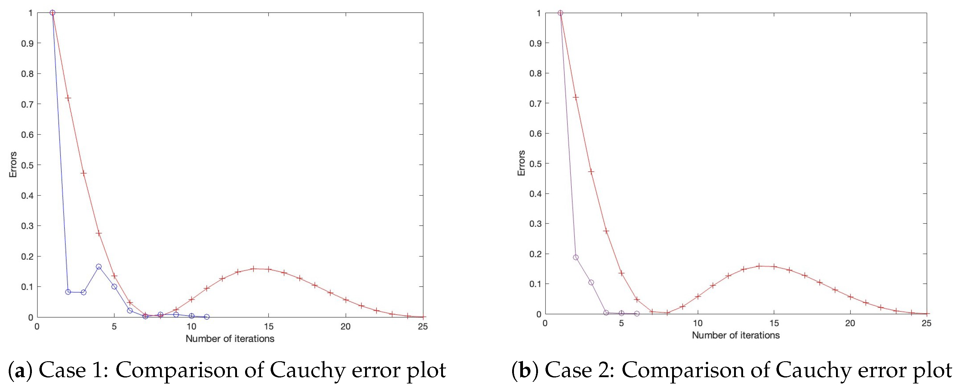
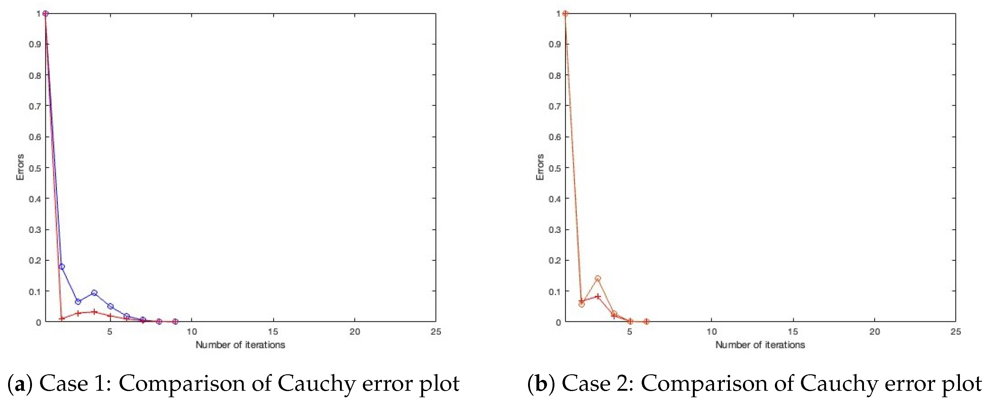
• Case 1: Define $T_{1}y\left(t\right)={\displaystyle \frac{2}{3}}y\left(t\right)$, with initial settings $y_0=sin\left(t\right)-2,x_0=t^2$ and $x_1=t^2-1$.
• Case 2: Define $T_{2}y\left(t\right)={\displaystyle \frac{1}{4}}y\left(t\right)$, with initial settings $y_0=sin\left(t\right)-2,x_0=t^2$ and $x_1=t^2-1$.
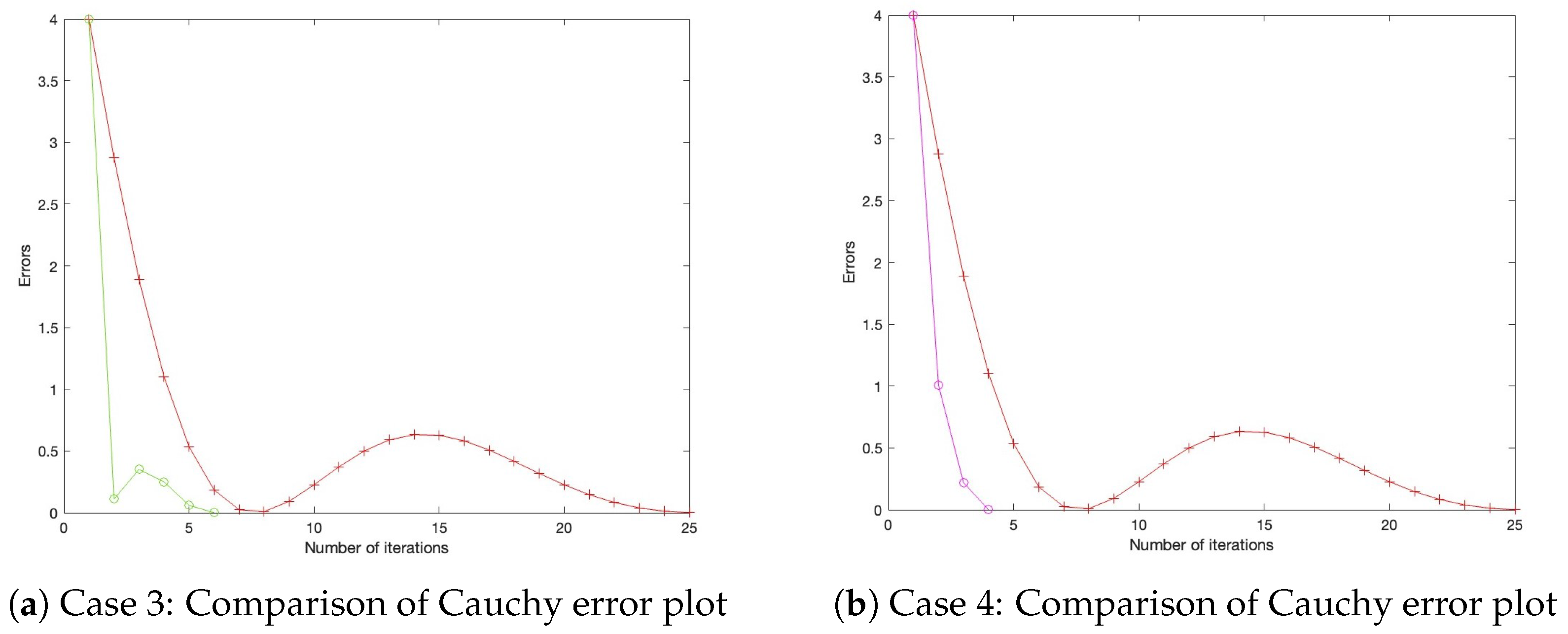
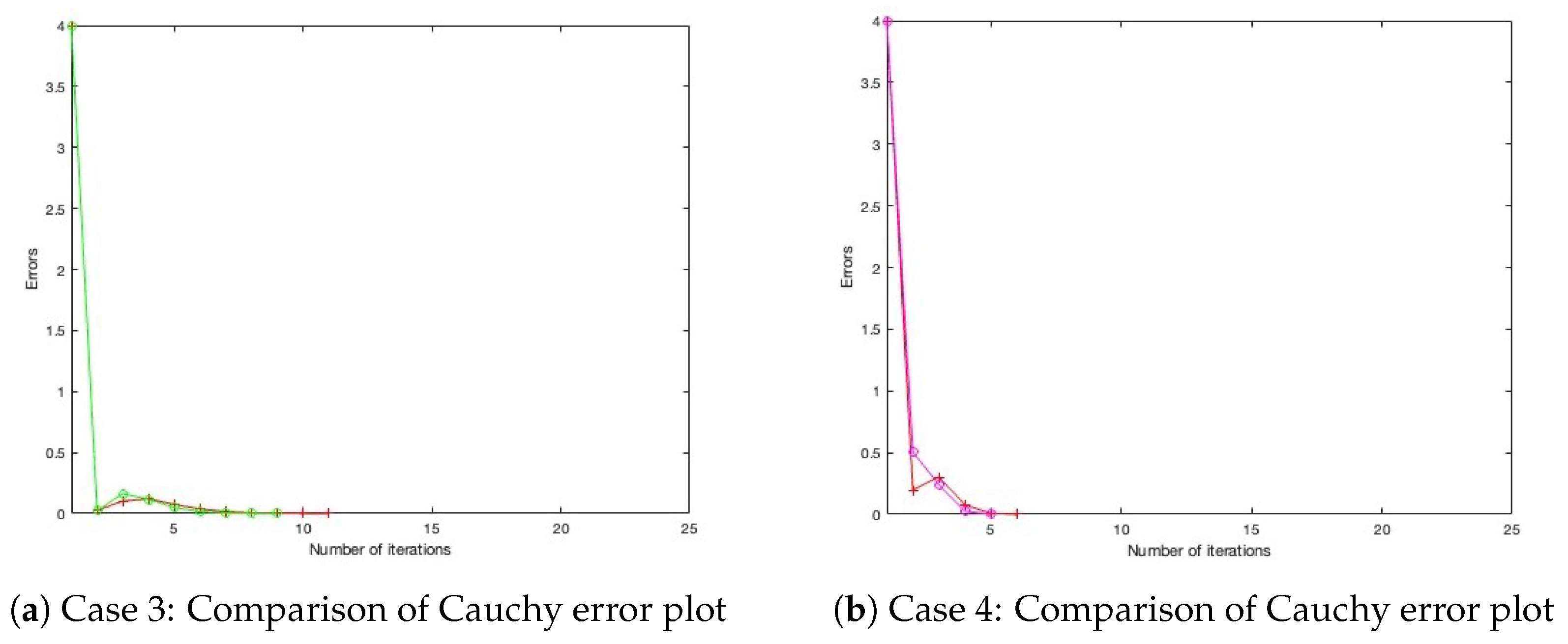
• Case 3: Define $T_{1}y\left(t\right)={\displaystyle \frac{2}{3}}y\left(t\right)$, with initial settings $y_0=e^t,x_0=t^2-1$ and $x_1=t^2+1$.
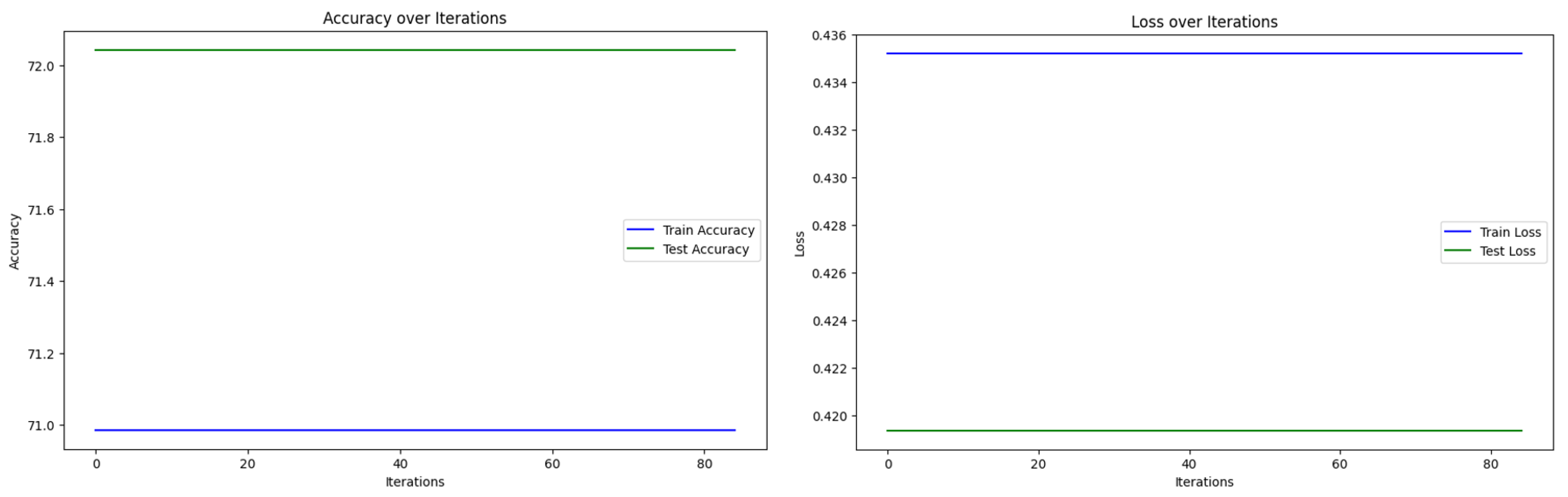
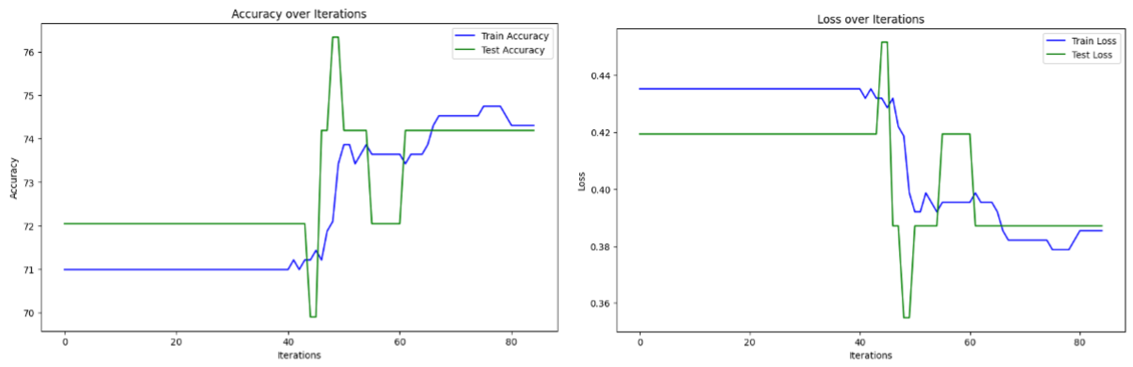
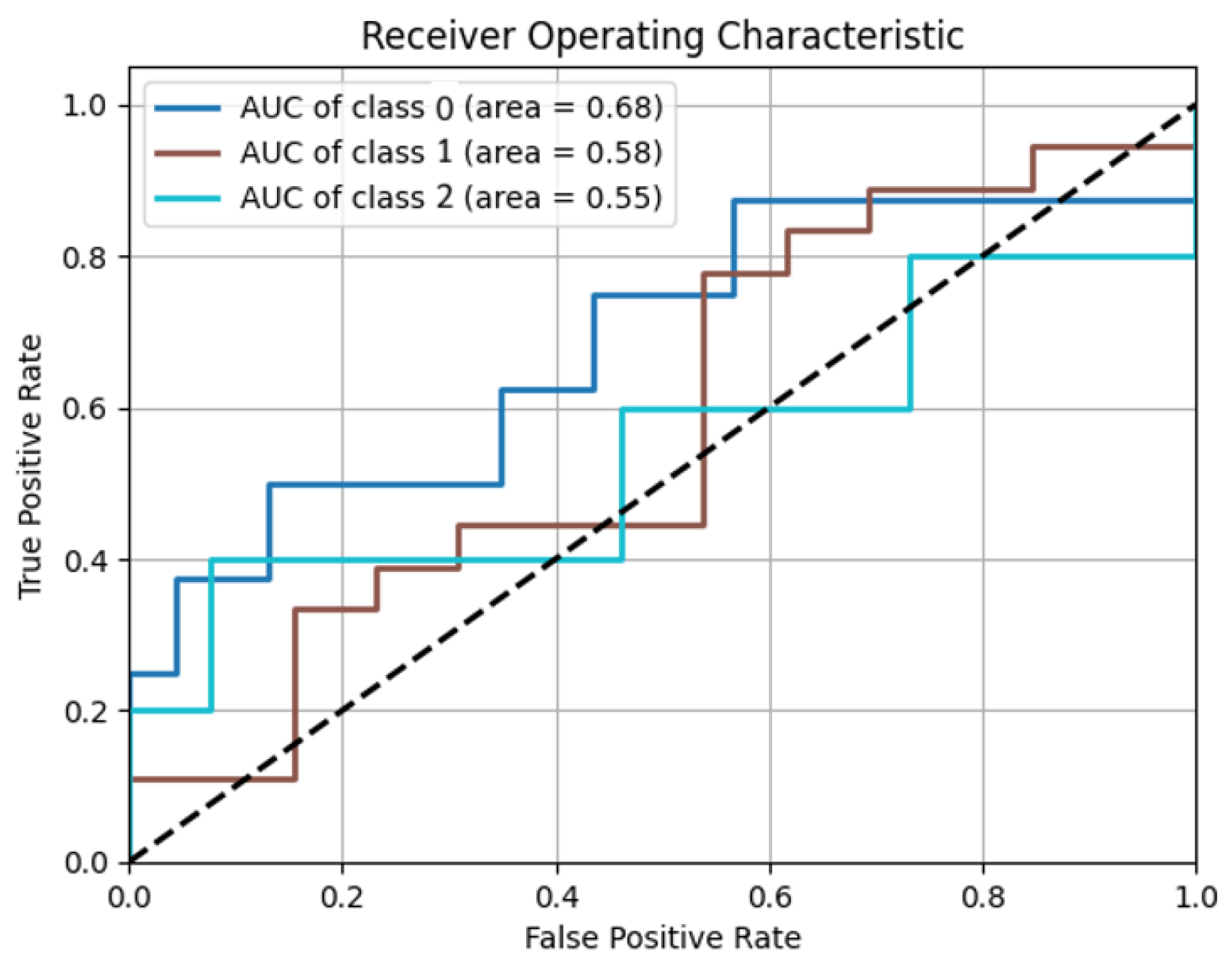
• Case 4: Define $T_{2}y\left(t\right)={\displaystyle \frac{1}{4}}y\left(t\right)$, with initial settings $y_0=e^t,x_0=t^2-1$ and $x_1=t^2+1$. All parameters for Algorithm 1, as well as those for the benchmark algorithm from the literature, are configured under three distinct settings, as presented in

  Table 1. Setting parameters.

  	${\mathit{\alpha }}^{\mathit{k}}$	${\mathit{\beta }}^{\mathit{k}}$	$\mathit{\theta }$	$\mathit{\delta }$
  Algorithm 1	0.9	0.5	0.9	0.01
  Algorithm of Mainge [9]	0.9	-	0.9	-

  ,

  Table 2. Setting parameters.

  	${\mathit{\alpha }}^{\mathit{k}}$	${\mathit{\beta }}^{\mathit{k}}$	$\mathit{\theta }$	$\mathit{\delta }$
  Algorithm 1	0.6	0.3	0.6	0.05
  Algorithm of Mainge [9]	0.6	-	0.6	-

  and

  Table 3. Setting parameters.

  	${\mathit{\alpha }}^{\mathit{k}}$	${\mathit{\beta }}^{\mathit{k}}$	$\mathit{\theta }$	$\mathit{\delta }$
  Algorithm 1	0.3	0.7	0.3	0.005
  Algorithm of Mainge [9]	0.3	-	0.3	-

  , with their corresponding Cauchy plot comparisons shown in Figure 1, Figure 2, Figure 3, Figure 4, Figure 5 and Figure 6.

Remark 1. 

The numerical results in Figure 1, Figure 2, Figure 3, Figure 4, Figure 5 and Figure 6, corresponding to the parameter settings in Table 1, Table 2 and Table 3, consistently demonstrate that Algorithm 1 achieves faster convergence with fewer iterations than Mainge’s method across all four test cases.

4. Application to Data Classification Problem

Urinary tract infections (UTIs) represent one of the most prevalent infectious diseases globally, affecting approximately 150 million individuals annually and imposing substantial healthcare and economic burdens worldwide. These infections, characterized by microbial invasion and colonization of the normally sterile urinary tract, demonstrate remarkable clinical heterogeneity ranging from asymptomatic bacteriuria to life-threatening urosepsis. Escherichia coli remains the predominant causative pathogen, accounting for 75–85% of uncomplicated UTIs, followed by other Enterobacteriaceae, Enterococcus species, and Staphylococcus saprophyticus.

The pathophysiology of UTIs involves complex molecular mechanisms including bacterial adherence via specialized pili, the invasion of uroepithelial cells, the formation of intracellular bacterial communities, and the establishment of quiescent reservoirs that contribute to recurrence patterns. Host defense mechanisms encompass mechanical clearance through urine flow, antimicrobial peptide secretion, and innate immune responses, which successful uropathogens have evolved sophisticated strategies to circumvent.

Timely and accurate classification of UTIs into uncomplicated, complicated, recurrent, or healthcare-associated forms remains pivotal for guiding evidence-based diagnosis and management strategies. Uncomplicated UTIs occur in healthy individuals with normal urinary tract anatomy and function, while complicated UTIs involve patients with predisposing factors such as structural abnormalities, immunocompromise, or indwelling catheters. Recurrent UTIs, defined as three or more episodes within 12 months or two within 6 months, affect 20–30% of women following initial infection and significantly impact quality of life. Healthcare-associated UTIs, particularly catheter-associated infections, represent the most common nosocomial infection and carry substantial morbidity and mortality risks.

Such systematic stratification enables targeted antimicrobial therapy, reduces treatment failure rates, and mitigates the growing threat of antimicrobial resistance. Furthermore, standardized classification frameworks enhance research comparability, inform epidemiological surveillance, and support evidence-based clinical practice guideline development.

The integration of machine learning and artificial intelligence technologies into UTI prediction and management represents a transformative advancement in precision medicine approaches to infectious disease care. Predictive modeling systems utilizing comprehensive clinical datasets can significantly enhance diagnostic accuracy, optimize treatment selection, and improve patient outcomes through early intervention strategies.

Advanced data classification algorithms can analyze multidimensional patient data including demographic characteristics, clinical symptoms, laboratory parameters, imaging findings, and historical infection patterns to predict UTI occurrence with remarkable precision. These predictive models demonstrate particular value in identifying high-risk patients who would benefit from prophylactic interventions, enabling proactive rather than reactive healthcare approaches.

The clinical applications of UTI prediction models extend across multiple healthcare domains. In emergency departments, rapid risk stratification tools can expedite triage decisions and guide empirical antibiotic selection, potentially reducing diagnostic delays and improving patient flow efficiency. For primary care providers, predictive algorithms can identify patients requiring closer monitoring or preventive interventions, facilitating personalized care plans that address individual risk factors.

In hospital settings, predictive models can enhance antimicrobial stewardship programs by identifying patients likely to harbor resistant organisms, enabling targeted therapy selection and reducing unnecessary broad-spectrum antibiotic use. This approach not only improves individual patient outcomes but also contributes to institutional efforts to combat antimicrobial resistance.

The economic implications of accurate UTI prediction are substantial, with potential cost savings through reduced emergency department visits, decreased hospitalization rates, and prevention of complications requiring intensive interventions. Early identification of recurrence-prone patients enables implementation of cost-effective prevention strategies, including behavioral modifications, prophylactic antimicrobials, or alternative interventions such as cranberry supplementation or probiotics.

Furthermore, predictive modeling can support clinical decision-making in special populations including pregnant women, elderly patients, and immunocompromised individuals, where UTI complications carry particularly serious consequences. By identifying high-risk cases early, healthcare providers can implement intensive monitoring protocols and aggressive treatment strategies to prevent progression to severe complications such as pyelonephritis or urosepsis. The integration of real-time clinical data with predictive algorithms also enables dynamic risk assessment, allowing healthcare systems to adapt prevention and treatment strategies based on evolving patient conditions and local epidemiological patterns. This adaptive approach represents a significant advancement toward truly personalized medicine in infectious disease management, ultimately improving patient outcomes while optimizing healthcare resource utilization.

To apply machine learning, we employ the Extreme Learning Machine (ELM) framework, as introduced by Huang et al. [34]. The training dataset is defined as $E:=\{({\mathbf{s}}_n,{\mathbf{r}}_n):{\mathbf{s}}_n\in {\mathbb{R}}^N,{\mathbf{r}}_n\in {\mathbb{R}}^M,n=1,2,...,P\}$, where ${\mathbf{s}}_n$ represents the input data, and ${\mathbf{r}}_n$ denotes the corresponding target. In a single-hidden layer feedforward neural network (SLFN) with R hidden nodes, the output function is given by

$${\displaystyle {\mathbf{Q}}_n=\sum _{k=1}^R{U}_{k}V(c_k{\mathbf{s}}_n+d_k),}$$

where V is the activation function, $c_k$ is the input weight matrix, $d_k$ is the bias vector, and $U_k$ is the output weight associated with the k-th hidden node. The hidden layer can be further defined as follows:

$$L=\left[\begin{array}{ccc}V(c_1{\mathbf{s}}_1+d_1)& \dots & V(c_R{\mathbf{s}}_1+d_R)\\ ⋮& \ddots & ⋮\\ V(c_1{\mathbf{s}}_P+d_1)& \dots & V(c_R{\mathbf{s}}_P+d_R)\end{array}\right]$$

To solve ELM is to find optimal output weight $U={[U_1,...,U_R]}^T$ such that $LU=T$, where $T={[{\mathbf{r}}_1,...,{\mathbf{r}}_P]}^T$ is the training data. In certain cases, finding $U=L^{†}T$, where $L^{†}$ is the Moore–Penrose generalized inverse of L. When the computation of $L^{†}$ is impractical, we can solve $LU=T$ by the following least square problems

$${\displaystyle \underset{U\in {\mathbb{R}}^R}{min}{\{\parallel LU-T\parallel }_2^2\}.}$$

(11)

To apply our algorithm to problem (11), we define the functions $\mathsf{p}(u,v)$ and $\mathsf{g}(u,v)$ as follows:

$$\mathsf{p}(u,v)=\left\{\begin{array}{c}0,\forall u,v\in \mathbb{P},\hfill \\ -1,\mathrm{otherwise},\hfill \end{array}\right.\mathsf{g}(u,v)=\left\{\begin{array}{c}0,\forall u,v\in \mathbb{Q},\hfill \\ -1,\mathrm{otherwise}.\hfill \end{array}\right.$$

Under these definitions, the proposed method reduces to the split-feasibility problem (SFP), originally introduced by Censor and Elfving [35], which consists of finding a point $u^{\ast }\in \mathbb{P}$ such that

$$\mathbb{A}{u}^{\ast }\in \mathbb{Q}$$

(12)

where $\mathbb{P},\mathbb{Q}$ are nonempty closed and convex subsets of ${\mathbb{R}}^N$ and ${\mathbb{R}}^M$, respectively, and $\mathbb{A}$ is an $M\times N$ real matrix. We create a model for our algorithm of the split-feasibility problem (12) to obtain results in machine learning (11).

• Least squares model

$${\displaystyle \underset{U\in \mathbb{P}}{min}\frac{1}{2}{\parallel P_{\mathbb{Q}}LU-LU\parallel }_2^2,}$$

setting $\mathbb{A}=L,\mathbb{Q}=\left\{T\right\}$, and $\mathbb{P}={\mathbb{H}}_1$.

In this study, we employ the multi-class cross-entropy loss function $\left(H\right(y,p\left)\right)$, where W denotes the total number of classes, and $y_k$ and $p_k$ represent the predicted probability for class k. The loss function is defined as follows:

$${\displaystyle H(y,p)=-\sum _{k=1}^W{y}_k·log\left(p_k\right).}$$

In evaluating model performance, precision reflects the ability to correctly identify positive instances, recall indicates the capacity to retrieve all relevant instances, and accuracy measures the proportion of total correct predictions. The mathematical formulations of these metrics are as follows [36]:

$$\mathrm{Precision}\left(\mathrm{Pre}\right)={\displaystyle \frac{TP}{TP+FP}}\times 100\%.$$

$$\mathrm{Recall}\left(\mathrm{Rec}\right)={\displaystyle \frac{TP}{TP+FN}}\times 100\%.$$

$$\mathrm{Accuracy}\left(\mathrm{Acc}\right)={\displaystyle \frac{TP+TN}{TP+FP+TN+FN}}\times 100\%.$$

Here, True Positives (TPs) refers to instances correctly predicted as positive; True Negatives (TNs) refers to instances correctly predicted as negative; False Positives (FPs) are incorrectly predicted as positive; and False Negatives (FNs) are incorrectly predicted as negative. Let P and N denote the number of actual positive and negative samples, respectively (e.g., malignant and benign cases). Furthermore, the F1-score—defined as the harmonic mean of precision and recall—is given by

$$\text{F1-Score}=2\left({\displaystyle \frac{\mathrm{Precision}\times \mathrm{Recall}}{\mathrm{Precision}+\mathrm{Recall}}}\right)\times 100\%.$$

All results are processed with Python 3.12.10 Visual Studio Code on a Lenovo laptop powered by AMD Ryzen™ 5 5600H CPU, 16 GB of RAM, and a GeForce RTX™ 3050 Laptop GPU. These data were collected at the University of Phayao Hospital, and we used training data of 90% and testing data of 10%. Clinical data were systematically extracted from the University of Phayao Hospital’s electronic health record system using comprehensive ICD-10 diagnostic codes. UTI cases were identified through specific codes including N39.0 (urinary tract infection and site unspecified), N30.0 (acute cystitis), N30.1-N30.9 (chronic and unspecified cystitis), N10 (acutepyelonephritis), N11.0-N11.9 (chronic pyelonephritis variants), and related complicated UTI codes (N12, N13.6, N15.1, and N34.0-N34.1). The Hospital Information System integration enabled automated extraction of patient demographics, clinical presentations, laboratory results, microbiological data, and treatment outcomes. Quality assurance measures included duplicate record identification, diagnostic code verification, and clinical correlation assessment to ensure data accuracy and research reproducibility.

Table 4. Data description.

	Minimum	Maximum	Mean	Median	Mode	Standard Deviation
UTI Type	0	2	1.3886	2	2	0.7712
Urinalysis Nitrite	0	1	0.1536	0	0	0.3611
Urinalysis Leukocyte Esterase	0	6	2.5663	3	3	1.0820
Age	1	98	55.8223	66	21	25.9832
Weight	8.5	90	51.9077	53	45	13.2993
BMI	13.2810	33.2700	21.7309	21.8750	15.6210	4.1219
Serum Vit D level	4.9600	62.4000	24.8455	23.6000	20.5000	8.4848
CBC hct	21	51	36.7169	37	36	5.1781
Height	69	185	153.7289	155	150	13.1780
Wbc	1	5	3.5904	4	3	1.0433
eGFR	0	281	139.4970	140.5000	66	82.2671
DM	0	1	0.3494	0	0	0.4775

is a description of each feature. These data contained 332 patients: 155 from class 2, 85 from class 1, and 59 from class 0. We select the hidden node as 600. The parameters ${\theta }^k$ and ${\delta }^k$ are assigned according to (9) and (10), respectively.

To select the parameter for all methods see in

Table 5. Setting parameters.

	L	$\mathit{\alpha }$	$\mathit{\beta }$	$\mathit{\delta }$	$\mathit{\theta }$
Algorithm 2—case 1	${\displaystyle \frac{0.9999}{max\left(eigenvalue\left(A^{T}A\right)\right)}}$	0.9	0.5	0.01	0.9
Algorithm 2—case 2	${\displaystyle \frac{0.9999}{max\left(eigenvalue\left(A^{T}A\right)\right)}}$	0.9	0.9	0.005	0.9
Algorithm 2—case 3	${\displaystyle \frac{0.9999}{max\left(eigenvalue\left(A^{T}A\right)\right)}}$	0.7	0.7	0.005	0.9
Algorithm of Suantai [16]	${\displaystyle \frac{0.9999}{max\left(eigenvalue\left(A^{T}A\right)\right)}}$	0.9	-	-	-
Algorithm of Yajai [12]	${\displaystyle \frac{0.9999}{max\left(eigenvalue\left(A^{T}A\right)\right)}}$	0.9	0.5	${\displaystyle \frac{2^{15}}{\parallel x^{k+1}-x^k{\parallel }^2+k^2+2^{15}}}$	${\displaystyle \frac{2^{12}}{\parallel x^{k+1}-x^k{\parallel }^5+k^5+2^{12}}}$

.

The proposed Algorithm 2 outperforms existing methods in all evaluation metrics, demonstrating both higher efficiency and accuracy see in

Table 6. Comparative efficiency of the proposed algorithm and existing method.

	Iterations	Computation Time (s)	Precision (%)	Recall (%)	F1-Score (%)	Accuracy (%)
Algorithm 2—case 1	85	13.4534	81.6667	77.7035	78.3688	78.4946
Algorithm 2—case 2	85	19.2733	79.6052	77.5362	78.1291	76.3441
Algorithm 2—case 3	85	20.4867	81.6667	77.7035	78.3688	78.4946
Algorithm of Suantai [16]	85	11.2421	52.6882	66.6667	58.8044	72.0430
Algorithm of Yajai [12]	85	46.9684	76.3266	73.6901	73.8186	74.1935

.

From Figure 7, Figure 8, Figure 9, Figure 10 and Figure 11, Figure 7 is evident that our Algorithm 2 achieves a well-fitted model, indicating that it effectively learns from the training data and generalizes well for classifying urinary tract infections.

The ROC curve Figure 12 illustrates the classification performance across three classes. Class 0 demonstrates the highest discriminative ability with an AUC of 0.68, indicating moderate predictive accuracy. Class 1 and Class 2 yield lower AUC values of 0.58 and 0.55, respectively, suggesting limited separability from random guessing. Despite these limitations, the model shows potential in distinguishing clinically relevant cases in Class 0, providing a promising foundation for future enhancements through targeted optimization and class-specific calibration.

The performance evaluation presented in Table 6 demonstrates significant improvements achieved by Algorithm 2 compared to the existing Algorithms of Suantai [16] and Yajai [12]. Algorithm 2 achieved superior accuracy of 78.4946% versus 72.0430% for the baseline algorithm, representing a clinically meaningful improvement of 6.45 percentage points. This enhancement translates to approximately 65 additional correct classifications per 1000 UTI cases, potentially preventing misdiagnoses that could lead to inappropriate treatment decisions or delayed interventions.

The precision metrics reveal Algorithm 2’s exceptional performance at 81.6667% compared to 52.6882% for the baseline, indicating substantially reduced false-positive rates. This 29-point improvement in precision is particularly crucial for UTI prediction as false positives can lead to unnecessary antibiotic prescriptions, contributing to antimicrobial resistance and patient exposure to potential adverse effects. The enhanced precision directly supports antimicrobial stewardship initiatives by ensuring that antibiotic interventions are recommended only for patients with genuine infection risk.

The recall performance shows Algorithm 2 achieving 77.7035% versus 66.6667% for the baseline algorithm, representing an 11-point improvement in sensitivity. This enhanced recall capability is clinically significant as it reduces false-negative rates, ensuring that fewer genuine UTI cases are missed. In clinical practice, missed UTI diagnoses can result in progression to serious complications including pyelonephritis, sepsis, and chronic kidney disease, particularly in vulnerable populations such as elderly patients or those with diabetes.

The F1-score improvement from 58.8044% to 78.3688% demonstrates Algorithm 2’s superior balanced performance between precision and recall, indicating optimal trade-offs essential for clinical decision-support systems. This balanced optimization is crucial for UTI prediction models as healthcare providers require algorithms that minimize both missed diagnoses and unnecessary treatments. The computational efficiency gains are equally important for real-world implementation. Algorithm 2 requires only 85 iterations compared to 85 iterations for the baseline but achieves convergence in 13.4534 s versus 11.2421 s. While slightly slower, the marginal time increase is clinically acceptable given the substantial accuracy improvements, particularly in non-emergency clinical settings where decision support can be integrated into routine workflow.

The accuracy improvements translate to tangible clinical benefits across multiple healthcare domains. In emergency departments, the enhanced precision reduces unnecessary antibiotic prescriptions and diagnostic uncertainty, potentially decreasing patient length of stay and improving resource utilization. For primary care settings, improved recall ensures that high-risk patients receive appropriate preventive interventions or closer monitoring, potentially preventing costly emergency department visits and hospitalizations. The algorithm’s performance characteristics support implementation in clinical decision support systems where balanced accuracy is essential. The 6.45% accuracy improvement could prevent approximately 6450 misclassifications per 100,000 patients screened, representing substantial healthcare cost savings through reduced inappropriate treatments and prevented complications. Furthermore, the enhanced precision supports quality improvement initiatives by reducing false-positive alerts that can lead to alert fatigue among healthcare providers. These performance improvements demonstrate Algorithm 2’s potential for meaningful clinical impact, supporting evidence-based UTI prediction and management strategies that optimize patient outcomes while promoting responsible antimicrobial use in contemporary healthcare practice.

5. Conclusions

This study aimed to develop a double inertial Mann-type method for nonexpansive mappings to predict the risk of urinary tract infection (UTI) in individuals with vitamin D deficiency. Using a dataset composed of various clinical features, the Extreme Learning Machine (ELM) algorithm was employed for classification. Statistical analysis, including the Kruskal–Wallis and Mann–Whitney U tests, confirmed significant differences in serum vitamin D levels across different UTI groups. These findings suggest a potential link between vitamin D status and UTI risk. The results support the model’s applicability in identifying at-risk individuals and provide a basis for further investigation into AI-assisted UTI screening tools in clinical practice.

References

- Abdou, A.A.N. Fixed Point Theorems: Exploring Applications in Fractional Differential Equations for Economic Growth. Fractal Fract. 2024, 8, 243. [Google Scholar] [CrossRef]
- Batiha, I.; Aoua, L.; Oussaeif, T.; Ouannas, A.; lshorman, S.; Jebril, I.; Momani, S. Common fixed point theorem in non-Archimedean Menger PM-spaces using CLR property with application to functional equations. IAENG Int. J. Appl. Math. 2023, 53, 360–368. [Google Scholar]
- Chouhan, S.; Desai, B. Fixed-Point Theory and Its Some Real-Life Applications. In Research Highlights in Mathematics and Computer Science; Book Publisher International: Versailles, France, 2022; Volume 1, pp. 119–125. [Google Scholar] [CrossRef]
- Patriche, M. Bayesian abstract fuzzy economies, random quasi-variational inequalities with random fuzzy mappings and random fixed point theorems. Fuzzy Sets Syst. 2014, 245, 125–136. [Google Scholar] [CrossRef]
- Scarf, H. Fixed-point theorems and economic analysis. Am. Sci. 1983, 71, 289–296. [Google Scholar]
- Mann, W.R. Mean value methods in iteration. Proc. Am. Math. Soc. 1953, 4, 506–510. [Google Scholar] [CrossRef]
- Reich, S. Weak convergence theorems for nonexpansive mappings in Banach spaces. J. Math. Anal. Appl. 1979, 67, 274–276. [Google Scholar] [CrossRef]
- Polyak, B.T. Some methods of speeding up the convergence of iteration methods. USSR Comput. Math. Math. Phys. 1964, 4, 1–17. [Google Scholar] [CrossRef]
- Maingé, P.E. Convergence theorems for inertial KM-type algorithms. J. Comput. Appl. Math. 2008, 219, 223–236. [Google Scholar] [CrossRef]
- Iyiola, O.S.; Shehu, Y. Convergence results of two-step inertial proximal point algorithm. Appl. Numer. Math. 2022, 182, 57–75. [Google Scholar] [CrossRef]
- Yao, Y.; Iyiola, O.S.; Shehu, Y. Subgradient extragradient method with double inertial steps for variational inequalities. J. Sci. Comput. 2022, 90, 71. [Google Scholar] [CrossRef]
- Yajai, W.; Kankam, K.; Yao, J.C.; Cholamjiak, W. A double inertial embedded modified S-iteration algorithm for nonexpansive mappings: A classification approach for lung cancer detection. Commun. Nonlinear Sci. Numer. Simul. 2025, 150, 108978. [Google Scholar] [CrossRef]
- Moudafi, A. Split monotone variational inclusions. J. Optim. Theory Appl. 2011, 150, 275–283. [Google Scholar] [CrossRef]
- Witthayarat, U.; Abdou, A.; Cho, Y. Shrinking projection methods for solving split equilibrium problems and fixed point problems for asymptotically nonexpansive mappings in Hilbert spaces. Fixed Point Theory Appl. 2015, 2015, 200. [Google Scholar] [CrossRef]
- Gebrie, A.; Wangkeeree, R. Hybrid projected subgradient-proximal algorithms for solving split equilibrium problems and split common fixed point problems of nonexpansive mappings in Hilbert spaces. Fixed Point Theory Appl. 2018, 2018, 5. [Google Scholar] [CrossRef]
- Suantai, S.; Cholamjiak, P.; Cho, Y.J.; Cholamjiak, W. On solving split equilibrium problems and fixed point problems of nonspreading multi-valued mappings in Hilbert spaces. Fixed Point Theory Appl. 2016, 2016, 35. [Google Scholar] [CrossRef]
- Li, Y.; Zhang, C.; Wang, Y. On solving split equilibrium problems and fixed point problems of α-nonexpansive multi-valued mappings in Hilbert spaces. Fixed Point Theory 2023, 24, 2. [Google Scholar]
- Bnouhachem, A. Strong convergence algorithm for split equilibrium problems and hierarchical fixed point problems. Sci. World J. 2014, 2014, 390956. [Google Scholar] [CrossRef]
- Kangtunyakarn, A. Hybrid algorithm for finding common elements of the set of generalized equilibrium problems and the set of fixed point problems of strictly pseudo-contractive mapping. Fixed Point Theory Appl. 2011, 2011, 274820. [Google Scholar] [CrossRef]
- Kazmi, K.R.; Rizvi, S.H. Iterative approximation of a common solution of a split equilibrium problem, a variational inequality problem and a fixed point problem. J. Egypt. Math. Soc. 2013, 21, 44–51. [Google Scholar] [CrossRef]
- Alansari, M.; Kazmi, K.R.; Ali, R. Hybrid iterative scheme for solving split equilibrium and hierarchical fixed point problems. Optim. Lett. 2020, 14, 2379–2394. [Google Scholar] [CrossRef]
- Harisa, S.A.; Khan, M.A.A.; Mumtaz, F. Shrinking Cesàro means method for the split equilibrium and fixed point problems in Hilbert spaces. Adv. Difference Equ. 2020, 2020, 345. [Google Scholar] [CrossRef]
- Inthakon, W.; Niyamosot, N. The split equilibrium problem and common fixed points of two relatively quasi-nonexpansive mappings in Banach spaces. J. Nonlinear Convex Anal. 2019, 20, 685–702. [Google Scholar]
- Jolaoso, L.O.; Karahan, I. A general alternative regularization method with line search technique for solving split equilibrium and fixed point problems in Hilbert spaces. J. Comput. Appl. Math. 2020, 391, 105150. [Google Scholar] [CrossRef]
- Petrot, N.; Rabbani, M.; Khonchaliew, M.; Dadashi, V. A new extragradient algorithm for split equilibrium problems and fixed point problems. J. Inequal. Appl. 2019, 2019, 137. [Google Scholar] [CrossRef]
- Yajai, W.; Nabheerong, P.; Cholamjiak, W. A double inertial Mann algorithm for split equilibrium problems application to breast cancer screening. J. Nonlinear Convex Anal. 2024, 25, 1697–1716. [Google Scholar]
- Blum, E.; Oettli, W. From optimization and variational inequalities to equilibrium problems. Math. Stud. 1994, 63, 123–145. [Google Scholar]
- Combettes, P.L.; Hirstoaga, S.A. Equilibrium programming in Hilbert spaces. J. Nonlinear Convex Anal. 2005, 6, 117–136. [Google Scholar]
- Ofoedu, E.U. Strong convergence theorem for uniformly L-Lipschitzian asymptotically pseudocontractive mapping in real Banach space. J. Math. Anal. Appl. 2006, 321, 722–728. [Google Scholar] [CrossRef]
- Goebel, K.; Kirk, W.A. Topics in Metric Fixed Point Theory; Cambridge University Press: Cambridge, UK, 1990. [Google Scholar]
- Opial, Z. Weak convergence of the sequence of successive approximations for nonexpansive mappings. Bull. Amer. Math. Soc. 1967, 73, 235–240. [Google Scholar] [CrossRef]
- Combettes, P.L. The convex feasibility problem in image recovery. Adv. Imaging Electron Phys. 1996, 95, 155–270. [Google Scholar]
- Byrne, C.; Censor, Y.; Gibali, A.; Reich, S. The split common null point problem. J. Nonlinear Convex Anal. 2012, 13, 759–775. [Google Scholar]
- Huang, G.B.; Zhu, Q.Y.; Siew, C.K. Extreme learning machine: Theory and applications. Neurocomputing 2006, 70, 489–501. [Google Scholar] [CrossRef]
- Censor, Y.; Elfving, T. A multiprojection algorithm using Bregman projections in a product space. Numer. Algorithms 1994, 8, 221–239. [Google Scholar] [CrossRef]
- Thomas, T.; Pradhan, N.; Dhaka, V.S. Comparative analysis to predict breast cancer using machine learning algorithms: A survey. In Proceedings of the 2020 International Conference on Inventive Computation Technologies (ICICT), Pune, India, 26–28 February 2020; pp. 192–196. [Google Scholar]