Graph-Regularized Orthogonal Non-Negative Matrix Factorization with Itakura–Saito (IS) Divergence for Fault Detection

Abstract

In modern industrial environments, quickly and accurately identifying faults is crucial for ensuring the smooth operation of production processes. Non-negative Matrix Factorization (NMF)-based fault detection technology has garnered attention due to its wide application in industrial process monitoring and machinery fault diagnosis. As an effective dimensionality reduction tool, NMF can decompose complex datasets into non-negative matrices with practical and physical significance, thereby extracting key features of the process. This paper presents a novel approach to fault detection in industrial processes, called Graph-Regularized Orthogonal Non-negative Matrix Factorization with Itakura–Saito Divergence (GONMF-IS). The proposed method addresses the challenges of fault detection in complex, non-Gaussian industrial environments. By using Itakura–Saito divergence, GONMF-IS effectively handles data with probabilistic distribution characteristics, improving the model’s ability to process non-Gaussian data. Additionally, graph regularization leverages the structural relationships among data points to refine the matrix factorization process, enhancing the robustness and adaptability of the algorithm. The incorporation of orthogonality constraints further enhances the independence and interpretability of the resulting factors. Through extensive experiments, the GONMF-IS method demonstrates superior performance in fault detection tasks, providing an effective and reliable tool for industrial applications. The results suggest that GONMF-IS offers significant improvements over traditional methods, offering a more robust and accurate solution for fault diagnosis in complex industrial settings.

1. Introduction

In the current era dominated by vast amounts of data, data-centric fault detection technology has become an indispensable part of modern industrial systems. The rapid and precise identification of potential issues is crucial for minimizing production disruptions, extending equipment lifespan, and safeguarding employee safety. Fault detection methods can generally be categorized into three main types based on their technical approaches: model-based methods, signal-based methods, and data-driven methods. Model-based methods rely on accurate mathematical models of the system; they perform well when the models are precise but face limitations when dealing with complex or unknown systems. Signal-based methods require high-quality input signals and are susceptible to external noise, which affects their stability and reliability. In contrast, data-driven methods do not depend on specific system models. Instead, they leverage large volumes of historical data to train machine learning models that can identify both normal operating patterns and fault modes. This approach offers significant adaptability and flexibility, enabling effective fault detection by comparing real-time data with training data. Traditional data-driven methods include Principal Component Analysis (PCA) and Independent Component Analysis (ICA), both of which assist in identifying fault patterns by extracting key features from the data. PCA transforms the data into a new coordinate system through linear transformation, where the first principal component corresponds to the direction of maximum variance in the data projection, the second principal component represents the direction of the second largest variance, and so on. On the other hand, ICA is a computational method used to decompose multivariate signals or datasets into statistically independent non-Gaussian signal sources. A promising technique known as Non-negative Matrix Factorization (NMF) has gained significant attention in the field of data-driven fault detection in recent years. The innovation of this method lies in its ability to decompose observed industrial process data under non-negativity constraints, not only effectively uncovering latent features in system operations but also yielding decomposition results that have clear physical interpretations [1,2]. Traditional Non-negative Matrix Factorization (NMF) methods still exhibit notable limitations when applied to complex industrial scenarios. On one hand, they struggle to effectively handle processes characterized by non-Gaussian distributions. On the other hand, these methods often fail to adequately capture the similarity and structural relationships among data points, which hinders further improvement in feature extraction performance. This is especially so when dealing with complex operating condition data that exhibit probabilistic distribution characteristics; the current NMF algorithms require further enhancement in terms of accuracy and robustness.

In 1999, Lee and Seung pioneered the theoretical framework of Non-negative Matrix Factorization (NMF) and proposed an associated optimization algorithm for matrix decomposition [3]. As research progressed, numerous improved variants of NMF were developed [4,5,6]. Among these advancements, Cai’s research team introduced a regularization strategy for NMF within a theoretical graph framework, leading to the development of the Graph-regularized NMF (GNMF) method [7]. Meanwhile, Berahmand et al. (2025) comprehensively reviewed the application of Spectral Clustering in high-dimensional data clustering in the article, particularly emphasizing the key role of Graph Structure Learning (GSL) in improving clustering performance [8]. Choi proposed the Orthogonal NMF (ONMF) model by incorporating orthogonality constraints into the original formulation [9,10]. Saberi-Movahed et al. (2024) together provided a comprehensive review of NMF in the field of dimensionality reduction, including its applications in feature extraction and feature selection [11]. Chen et al.(2022) provides a comprehensive overview of Deep Non-negative Matrix Factorization (Deep NMF) [12]. These enhanced NMF algorithms have demonstrated significant advantages in various engineering applications [13,14,15,16]. In the field of industrial fault diagnosis, Li was among the first to introduce NMF into fault detection. The innovation lies in the use of two statistical indicators—Hotelling’s $T^2$ and squared prediction error (SPE)—for fault feature extraction, combined with kernel-density estimation to determine control thresholds [17]. In the field of fault detection based on graph neural networks, Xiao proposed a bearing fault detection method based on graph neural networks, which uses graph autoencoders for unsupervised anomaly detection, significantly improving the accuracy of fault detection [18]. The effectiveness of these approaches was validated on the benchmark Tennessee Eastman Process (TEP) platform. Building upon this foundation, subsequent studies have proposed several improved models, including the Deep NMF (DNMF), Structured Joint Sparsity NMF (SJSNMF), and Structured Joint Sparsity Orthogonal NMF (SJSONMF) frameworks. These developments have achieved notable success in practical fault-diagnosis tasks [19,20,21,22].

The GONMF-IS framework significantly enhances fault detection performance by integrating advanced techniques such as Non-negative Matrix Factorization (NMF), graph regularization, orthogonal constraints, and the Itakura–Saito divergence (IS divergence). Within this framework, graph regularization delves into the internal similarity relationships within the data, providing the model with rich structural information. This precise capture of intrinsic data correlations enables the model to better understand the overall data distribution, laying a solid foundation for subsequent fault detection. At the same time, the introduction of orthogonal constraints further optimizes the feature extraction process. By ensuring the independence of extracted features, these constraints effectively eliminate redundant information among features and notably improve the model’s interpretability. This independence allows each feature to clearly reflect specific characteristics of the data, offering more accurate and reliable insights for fault detection. Furthermore, the GONMF-IS framework innovatively incorporates the Itakura–Saito divergence (IS divergence) as a core optimization tool [23,24,25]. The IS divergence is particularly effective in measuring and adjusting the discrepancies between different data distributions, excelling at capturing subtle variations within complex datasets. Its sensitivity to distributional differences enhances the model’s ability to distinguish between normal and faulty conditions. As a result, the GONMF-IS framework not only improves the accuracy of fault detection but also strengthens the robustness and stability of the detection outcomes.

Future research will focus on exploring the synergistic optimization mechanisms between Non-negative Matrix Factorization (NMF) and multi-dimensional divergence measures. This includes the development of novel divergence metrics, the design of adaptive algorithms for optimal measure selection, and the enhancement of model interpretability and visualization capabilities. Additionally, efforts will be directed toward improving the model’s robustness against noise and interference. Such investigations aim to advance the theoretical foundation of divergence-based NMF methods while also offering innovative solutions for industrial fault diagnosis. By leveraging cutting-edge methodologies, this line of research is expected to provide reliable technical support for ensuring the stable operation and secure control of complex industrial systems.

2. Preliminaries

Definition 1.

The Frobenius norm of a matrix, denoted as ${\parallel \mathit{X}\parallel }_F$, is defined as the square root of the sum of the squares of all its elements. In mathematical terms, it is expressed as follows:

$${\parallel \mathit{X}\parallel }_F=\sqrt{{\sum }_{i=1}^m{\sum }_{j=1}^n{\left|x_{ij}\right|}^2}$$

where $x_{ij}$ is the element in the i-th row and j-th column of matrix $\mathit{X}$.

Definition 2.

For matrix $\mathit{X}\in R^{m\ast n}$, the 2,1-norm is computed as the sum of the Euclidean norms (i.e., 2-norms) of each individual row in the matrix. In other words, it computes the Euclidean norm across the columns for every row and then sums these values together. Mathematically, it is expressed as follows:

$${\parallel \mathit{X}\parallel }_{2,1}={\sum }_{i=1}^m{\left({\sum }_{j=1}^n{\left|x_{ij}\right|}^2\right)}^{1/2}$$

Definition 3.

The Kullback–Leibler divergence (KL divergence), also known as relative entropy, is a measure of how one probability distribution $\mathit{P}$ is different from a second, reference probability distribution $\mathit{Q}$. It is defined as an asymmetric measure of the difference between the two distributions. The formula for KL divergence is as follows:

$$D_{KL}(\mathit{P}\Vert \mathit{Q})={\sum }_{x}P\left(x\right)log{\displaystyle \frac{\mathit{P}\left(x\right)}{\mathit{Q}\left(x\right)}}$$

Definition 4.

The Jensen–Shannon divergence (JS divergence) is a method for measuring the similarity between two probability distributions. It is defined based on the Kullback–Leibler divergence (KL divergence), but unlike KL divergence, JS divergence is symmetric and finite, even when the two distributions do not intersect. The definition of JS divergence is as follows:

$$D_{JS}(\mathit{P}\Vert \mathit{Q})={\displaystyle \frac{1}{2}}{D}_{KL}(\mathit{P}\Vert \mathit{M})+{\displaystyle \frac{1}{2}}{D}_{KL}(\mathit{Q}\Vert \mathit{M})$$

where $\mathit{P}$ and $\mathit{Q}$ are two probability distributions. $\mathit{M}$ is the average distribution of $\mathit{P}$ and $\mathit{Q}$, defined as follows: $\mathit{M}={\displaystyle \frac{1}{2}}(\mathit{P}+\mathit{Q})$.

Definition 5.

The Itakura–Saito (IS) Divergence is a non-symmetric measure used to quantify the difference between two spectra or probability distributions. It is defined as follows:

$$D_{IS}(\mathit{P}\Vert \mathit{Q})={\displaystyle \frac{\mathit{P}}{\mathit{Q}}}-log{\displaystyle \frac{\mathit{P}}{\mathit{Q}}}-1.$$

3. Related Works

3.1. Non-Negative Matrix Factorization

Given a non-negative matrix $\mathit{V}\in {\mathbb{R}}^{m\times N}$ where $\mathit{V}\ge 0$, the goal of Non-negative Matrix Factorization is to decompose $\mathit{V}$ into the product of two non-negative matrices $\mathit{A}\in {\mathbb{R}}^{m\times r}$ and $\mathit{S}\in {\mathbb{R}}^{r\times N}$, it can be described as the following optimization problem:

$$\underset{A,S}{min}{∥\mathit{V}-\mathit{A}\mathit{S}∥}_F^2\mathrm{s}.\mathrm{t}.\mathit{A}\ge 0, \mathit{S}\ge 0.$$

(1)

Here, $\mathit{A}$ and $\mathit{S}$ are non-negative matrices, and r is a positive integer representing the rank of the decomposition.

3.2. Variants of Non-Negative Matrix Factorization

The objective function for NMF with KL divergence can be formulated as follows:

$$\underset{\mathit{A},\mathit{S}}{min}{D}_{KL}(\mathit{V}\parallel \mathit{A}\mathit{S})\mathrm{s}.\mathrm{t}.\mathit{A}\ge 0, \mathit{S}\ge 0.$$

where $\mathit{V}$ is the original non-negative matrix, $\mathit{A}$ and $\mathit{S}$ are the non-negative matrices to be found, and denotes the Kullback–Leibler divergence [26,27]. The KL divergence between two matrices $\mathit{A}$ and $\mathit{B}$ is defined element-wise as follows:

$$D_{KL}(\mathit{A}\parallel \mathit{B})=\sum _{i,j}{\mathit{A}}_{ij}log{\displaystyle \frac{{\mathit{A}}_{ij}}{{\mathit{B}}_{ij}}}-\left({\mathit{A}}_{ij}-{\mathit{B}}_{ij}\right)$$

(2)

In the context of NMF, this can be written as follows:

$$D_{KL}(\mathit{V}\mid \mid \mathit{A}\mathit{S})=\sum _{i,j}{\mathit{V}}_{ij}log{\displaystyle \frac{{\mathit{V}}_{ij}}{{\left(\mathit{AS}\right)}_{ij}}}-({\mathit{V}}_{ij}-{\left(\mathit{AS}\right)}_{ij})$$

(3)

The optimization problem is to find $\mathit{A}$ and $\mathit{S}$ such that the above divergence is minimized, subject to the constraints that all elements of $\mathit{A}$ and $\mathit{S}$ are non-negative. GNMF incorporates graph regularization into the classical Non-negative Matrix Factorization (NMF) to better capture the local structure of the data, and its objective function can be expressed as follows [28,29]:

$$\begin{array}{c}\underset{A,S}{min}{\parallel \mathit{V}-\mathit{AS}\parallel }_F^2+\lambda tr\left(\mathit{S}\mathit{L}{\mathit{S}}^T\right)\\ \mathrm{s}.\mathrm{t}.\mathit{A}\ge 0, \mathit{S}\ge 0.\end{array}$$

(4)

where $\mathit{L}$ is the graph Laplacian matrix, and $\lambda$ is the regularization parameter. The graph Laplacian matrix is $\mathit{L}=\mathit{D}-\mathit{W}$, where $\mathit{D}$ is the degree matrix, and $\mathit{W}$ is the adjacency matrix constructed based on the distance or similarity between data points. The Itakura–Saito (IS) divergence is a metric commonly used in signal processing and information theory, especially in applications like linear predictive coding. The definition of IS divergence is as follows: $d\left(x\right|y)={\displaystyle \frac{x}{y}}-log{\displaystyle \frac{x}{y}}-1$. The nmf function incorporating the IS Divergence is as follows [23]:

$$\begin{array}{c}\underset{A,S}{min}{\displaystyle \frac{\mathit{V}}{\mathit{AS}}}-log{\displaystyle \frac{\mathit{V}}{\mathit{AS}}}-1.\\ \mathrm{s}.\mathrm{t}.\mathit{A}>0, \mathit{S}>0.\end{array}$$

(5)

Unlike the classical nmf model, here, the decomposed matrix $\mathit{A}$, $\mathit{S}$ is required to be greater than 0 and not equal to 0.

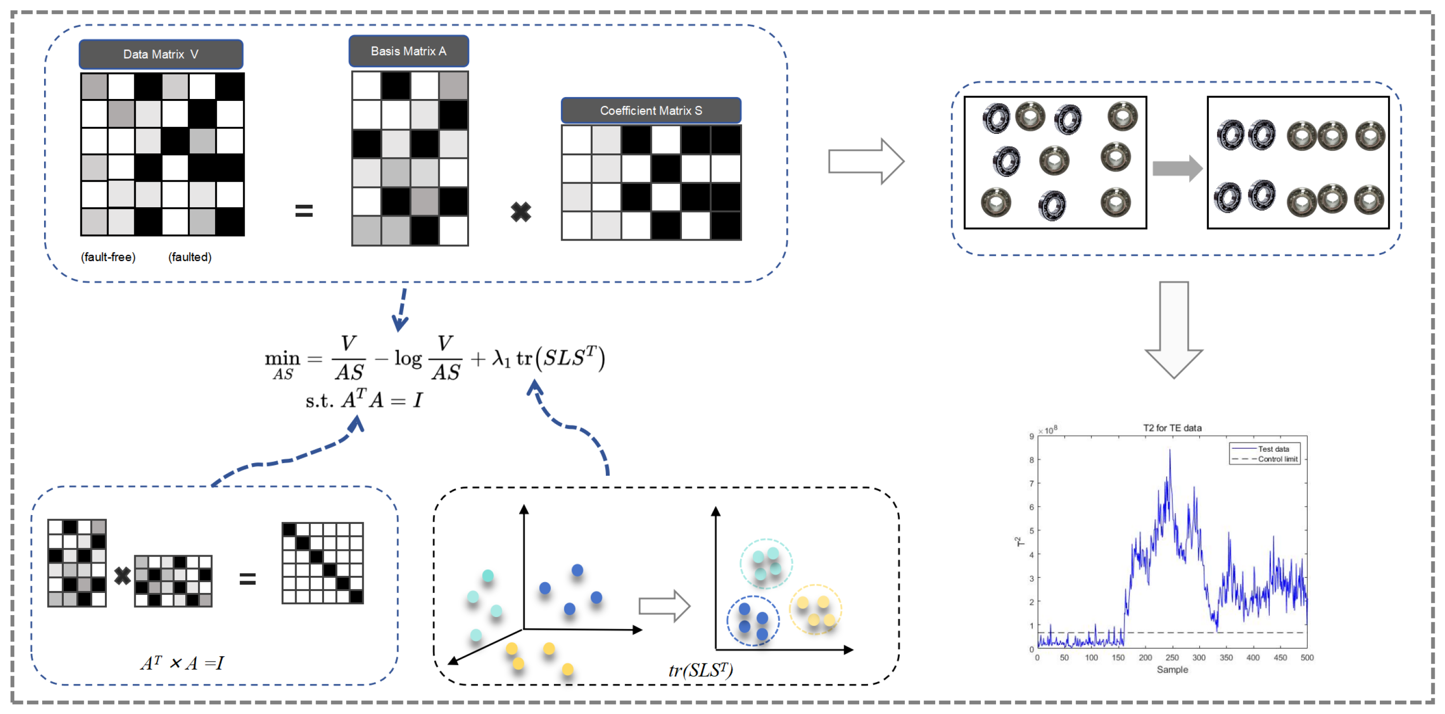
3.3. Model Construction

In this section, the paper presents an innovative model that integrates IS divergence into the framework of Non-negative Matrix Factorization (NMF), further incorporating a graph regularization term. The specific form of the model is as follows:

$$\begin{array}{c}\underset{A,S}{min}{\displaystyle \frac{\mathit{V}}{\mathit{AS}}}-log{\displaystyle \frac{\mathit{V}}{\mathit{AS}}}+\lambda tr\left(\mathit{S}\mathit{L}{\mathit{S}}^T\right).\\ \mathrm{s}.\mathrm{t}.{\mathit{A}}^{\mathit{T}}\mathit{A}=\mathit{I},\mathit{A}>0,\mathit{S}>0.\end{array}$$

(6)

KL divergence and Itakura–Saito divergence are both measures used to quantify the difference between probability distributions, but they differ in their mathematical forms, properties, and applications. KL divergence is widely used in machine learning and information theory, being sensitive to small changes in the tail of distributions and asymmetric when comparing different distributions. Itakura–Saito divergence, on the other hand, is particularly suited for handling non-negative data and is commonly used in speech recognition and audio processing. It is more robust to extreme values and is also asymmetric. Both are non-negative, but KL divergence is more sensitive to tail and outlier values, while Itakura–Saito divergence is better suited for signal-processing tasks. The model schematic is shown in Figure 1.

4. Optimization Process

Alternating Direction Method of Multipliers (ADMM) is an optimization method designed to minimize functions with multiple sets of variables, especially when these variables can be divided into distinct groups [30,31]. The algorithm works by iteratively optimizing each group of variables while holding the others constant. This technique is particularly effective for large-scale optimization tasks, as it reduces the computational complexity at each step. For Equation (8), the Alternating Direction Method of Multipliers (ADMM) algorithm is used to update variables one by one [32,33]. The initial formula for the objective function is as follows:

$$\begin{array}{cc}\hfill \underset{A,S}{min}& ={\displaystyle \frac{\mathit{V}}{\mathit{A}\mathit{S}}}-log{\displaystyle \frac{\mathit{V}}{\mathit{A}\mathit{S}}}+{\lambda }_{1}tr\left(\mathit{S}\mathit{L}{\mathit{S}}^{\mathit{T}}\right)\hfill \\ \hfill & \mathrm{s}.\mathrm{t}.\mathit{Z}=\mathit{AS}, {\mathit{A}}^{\mathit{T}}\mathit{A}=\mathit{I}, \mathit{A}>0, \mathit{S}>0.\hfill \end{array}$$

(7)

The associated augmented Lagrangian is as follows:

$$\begin{array}{cc}\hfill & L\left(\mathit{V},\mathit{A},\mathit{S},{\mathit{A}}_{+},{\mathit{S}}_{+},\mathit{N},\mathit{P},\mathit{Q},\mathit{Y}\right)=\hfill \\ \hfill & {\displaystyle \frac{\mathit{V}}{\mathit{Z}}}-log{\displaystyle \frac{\mathit{V}}{\mathit{Z}}}+{\lambda }_{1}tr\left(\mathit{S}\mathit{L}{\mathit{S}}^{\mathit{T}}\right)\hfill \\ \hfill & +〈\mathit{N},\mathit{Z}-\mathit{A}\mathit{S}〉+{\displaystyle \frac{\beta }{2}}{\parallel \mathit{Z}-\mathit{A}\mathit{S}\parallel }_F^2\hfill \\ \hfill & +〈\mathit{P},\mathit{A}-{\mathit{A}}_{+}〉+{\displaystyle \frac{\beta }{2}}{∥\mathit{A}-{\mathit{A}}_{+}∥}_F^2\hfill \\ \hfill & +〈\mathit{Q},\mathit{S}-{\mathit{S}}_{+}〉+{\displaystyle \frac{\beta }{2}}{∥\mathit{S}-{\mathit{S}}_{+}∥}_F^2\hfill \\ \hfill & +〈\mathit{Y},{\mathit{A}}^T\mathit{A}-\mathit{I}〉+{\displaystyle \frac{\beta }{2}}{∥{\mathit{A}}^T\mathit{A}-\mathit{I}∥}_F^2.\hfill \end{array}$$

(8)

4.1. Update ${\mathit{Z}}^{k+1}$, Fixed ${\mathit{A}}^k,{\mathit{S}}^k$

If other variables are fixed, the variable $\mathit{Z}$ subproblem can be written as follows:

$$\begin{array}{cc}\hfill \underset{A,S}{min}& {\displaystyle \frac{\mathit{V}}{\mathit{Z}}}-log{\displaystyle \frac{\mathit{V}}{\mathit{Z}}}+〈\mathit{N},\mathit{Z}-\mathit{A}\mathit{S}〉+\hfill \\ & {\displaystyle \frac{\beta }{2}}{\parallel \mathit{Z}-\mathit{A}\mathit{S}\parallel }_F^2\hfill \end{array}$$

(9)

The derivation of $\mathit{Z}$ yields the following equation:

$$\begin{array}{cc}\hfill \beta \left({\mathit{Z}}^3\right)-\beta \left({\mathit{Z}}^2\right)\mathit{A}\mathit{S}+\mathit{Z}-\mathit{V}& =0\hfill \end{array}$$

(10)

for this cubic equation with one variable, the Newton method is used to solve it in this paper.

4.2. Update ${\mathit{A}}^{k+1}$, Fixed ${\mathit{Z}}^{k+1},{\mathit{S}}^k$

For variable $\mathit{A}$ the subproblem can be written as follows:

$$\begin{array}{cc}\hfill \underset{W,H}{min}& 〈\mathit{N},\mathit{Z}-\mathit{A}\mathit{S}〉+{\displaystyle \frac{\beta }{2}}{\parallel \mathit{Z}-\mathit{A}\mathit{S}\parallel }_F^2\hfill \\ \hfill & +〈\mathit{P},\mathit{A}-{\mathit{A}}_{+}〉+{\displaystyle \frac{\beta }{2}}{∥\mathit{A}-{\mathit{A}}_{+}∥}_F^2\hfill \\ \hfill & +〈\mathit{Y},{\mathit{A}}^T\mathit{A}-\mathit{I}〉+{\displaystyle \frac{\beta }{2}}{∥{\mathit{A}}^T\mathit{A}-\mathit{I}∥}_F^2.\hfill \end{array}$$

(11)

The derivation of $\mathit{A}$ yields the following equation:

$$\begin{array}{c}\hfill \mathit{A}=\left(\mathit{N}{\mathit{S}}^T+\beta \mathit{Z}{\mathit{S}}^T+\beta {\mathit{A}}_{+}-\mathit{P}\right){\left(\beta \mathit{S}\left({\mathit{S}}^T\right)+\beta \mathit{I}+{\mathit{Y}}^T+\mathit{Y}\right)}^{-1}\end{array}$$

(12)

4.3. Update ${\mathit{S}}^{k+1}$, Fixed ${\mathit{Z}}^{k+1},{\mathit{A}}^{k+1}$

For variable $\mathit{S}$, the subproblem can be written as follows:

$$\begin{array}{cc}\hfill \underset{W,H}{min}& {\lambda }_{1}tr\left(\mathit{S}\mathit{L}{\mathit{S}}^{\mathit{T}}\right)\hfill \\ \hfill & +〈\mathit{N},\mathit{Z}-\mathit{A}\mathit{S}〉+{\displaystyle \frac{\beta }{2}}{\parallel \mathit{Z}-\mathit{A}\mathit{S}\parallel }_F^2\hfill \\ \hfill & +〈\mathit{Q},\mathit{S}-{\mathit{S}}_{+}〉+{\displaystyle \frac{\beta }{2}}{∥\mathit{S}-{\mathit{S}}_{+}∥}_F^2\hfill \end{array}$$

(13)

The derivation of $\mathit{S}$ yields the following equation:

$$\begin{array}{cc}\hfill \beta \left({\mathit{A}}^T\mathit{A}+\mathit{I}\right)\mathit{S}+\mathit{S}·2{\lambda }_1\mathit{L}& =\beta {\mathit{A}}^T\mathit{Z}+{\mathit{A}}^T\mathit{N}+\beta {\mathit{S}}_{+}-\mathit{Q}\hfill \end{array}$$

(14)

The above is a Sylvester equation that can be solved directly with a function in matlab.

4.4. Complexity Analysis

The computational complexity of the model mainly consists of two parts: the objective function and the constraints. In the objective function, the matrix multiplication $\mathit{AS}$ has a complexity of $O\left(mnk\right)$, while computing both requires $O\left(mn\right)$ operations. The term ${\lambda }_{1}tr\left({\mathit{SLS}}^{\mathit{T}}\right)$ involves a complexity of $O\left(k{n}^2\right)$. Therefore, the total complexity of the objective function is $O(mnk+mn+k{n}^2)$. Regarding the constraints, computing $\mathit{Z}=\mathit{AS}$ also takes $O\left(mnk\right)$, and evaluating ${\mathit{A}}^{\mathit{T}}\mathit{A}=\mathit{I}$ involves a complexity of $O(m{k}^2+k^2)$. Assuming the algorithm runs for t iterations, the overall computational complexity of the model is $O\left(t(mnk+mn+k{n}^2+m{k}^2+k^2)\right)$, indicating that the computational cost scales with the matrix dimensions $m,n,k$, the number of iterations t, and the structure of the graph Laplacian matrix $\mathit{L}$.

5. Simulation Experiments

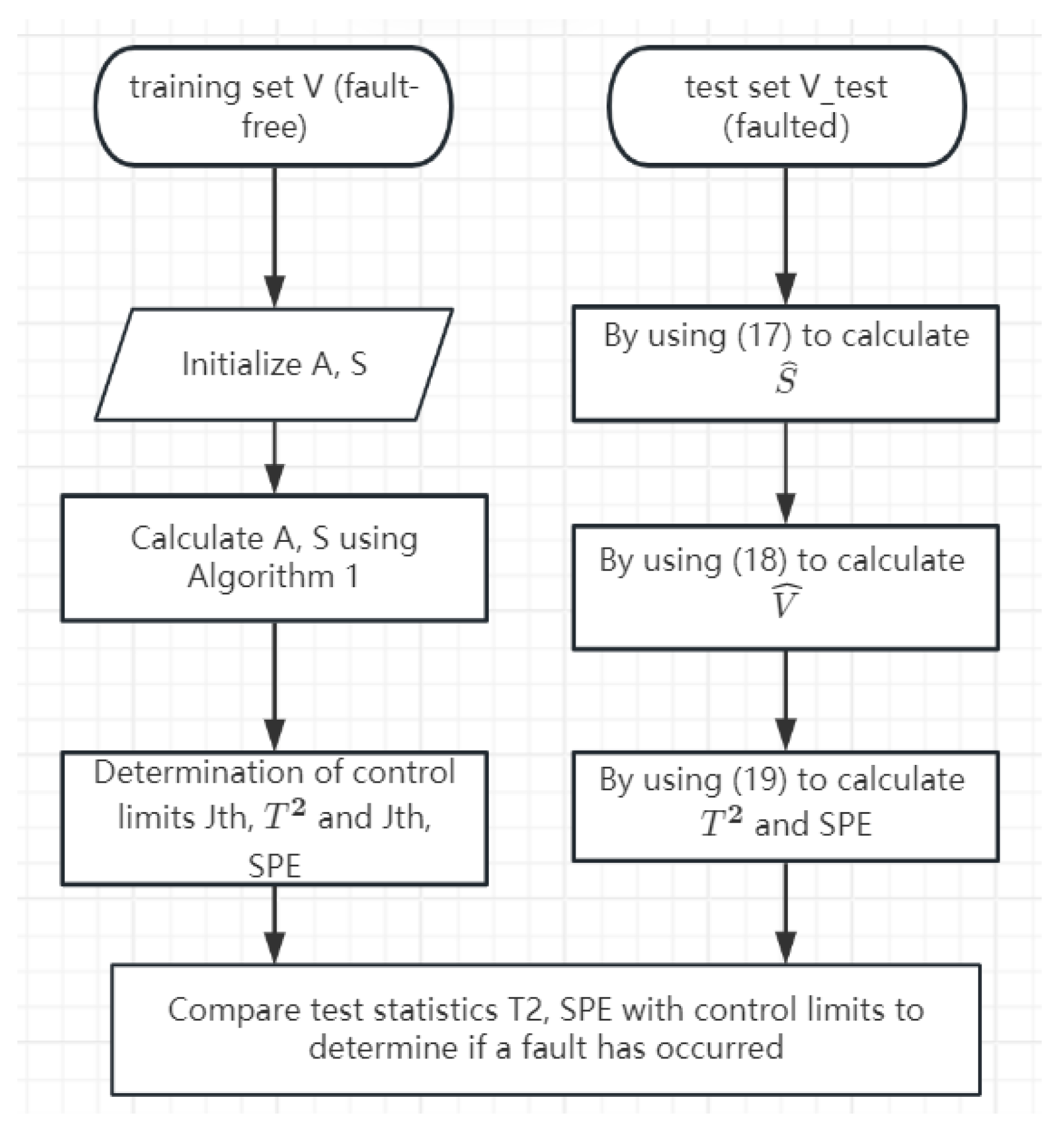
5.1. Fault Detection Process

This section describes the fault detection process based on (ISGONMF). By optimizing Algorithm 1, the decomposed matrices $\mathit{A}$ and $\mathit{S}$ are obtained, and the coefficient matrix $\mathit{S}$ serves as a low-rank approximation of the original data $\mathit{V}$, reflecting the state of the industrial process represented by $\mathit{V}$. When given a test set ${\mathit{V}}_{test}$, according to [17], the reconstruction $\widehat{\mathit{S}}$ of $\mathit{S}$ is expressed as follows:

$$\widehat{\mathit{S}}={\left({\mathit{A}}^T\mathit{A}\right)}^{-1}{\mathit{A}}^T{\mathit{V}}_{\mathrm{test}}={\mathit{A}}^T{\mathit{V}}_{\mathrm{test}}.$$

(15)

Subsequently, the monitoring model based on Non-negative Matrix Factorization (NMF) is formulated as follows:

$$\widehat{\mathit{V}}=\mathit{A}\widehat{\mathit{S}}.$$

(16)

Furthermore, there are two monitoring metrics: the $T^2$ statistic and the Squared Prediction Error ($SPE$) statistic, which are utilized to monitor the industrial process. These are defined as follows:

$$T^2={\widehat{\mathit{S}}}^T\widehat{\mathit{S}},SPE={({\mathit{V}}_{\mathrm{test}}-\widehat{\mathit{V}})}^T({\mathit{V}}_{\mathrm{test}}-\widehat{\mathit{V}}).$$

(17)

Use Kernel Density Estimation (KDE) to estimate the probability density function and calculate control limits. Assuming $x_i$ represents a sample set where each $x_i$ is independently and identically distributed as x according to the probability density function $p\left(x\right)$, the estimation of which can be expressed as follows:

$$\widehat{p}\left(x\right)={\displaystyle \frac{1}{nh}}\sum _{i=1}^{n}K\left({\displaystyle \frac{x-x_i}{h}}\right)$$

(18)

h represents the bandwidth, and $K(·)$ is the kernel function that meets ${\int }_{-\infty }^{+\infty }$ $K\left(x\right)dx=1$ and $K\left(x\right)\ge 0$. The Gaussian kernel function is selected for $K(·)$. Given the significant impact of bandwidth choice on $p\left(x\right)$ estimation, the optimal bandwidth h is determined by minimizing the mean integrated square error (MISE), which is expressed as follows:

$$h_{\mathrm{opt}}=1.06\sigma n^{-{\displaystyle \frac{1}{5}}}$$

(19)

As the training phase is completed offline, the online detection process is notably swift, ensuring the efficiency of the detection method. The NMF-based fault detection process is shown in Figure 2.

Algorithm 1. Algorithm for solving ISGONMF

Input: Sample matrix $\mathit{V}$, parameter ${\lambda }_1$, $\beta$, the rank of the decomposition k, iterations.

Initialize: ${\mathit{A}}_{\mathit{init}}$, ${\mathit{S}}_{\mathit{init}}$.

1. Calculated Diagonal matrix $\mathit{D}$.

2. Calculated Laplace matrix $\mathit{L}$.

3. For i = 1 to k

calculated gradient matrix ${\mathit{Z}}^{k+1}$ by Equation (10);

calculated gradient matrix ${\mathit{A}}^{k+1}$ by Equation (12);

calculated gradient matrix ${\mathit{S}}^{k+1}$ by Equation (14);

4. end for

Output ${\mathit{A}}^{k+1}, {\mathit{S}}^{k+1}$.

5.2. Application on the TEP

The TEP, developed by Eastman Chemical Company, aims to assess process control and monitoring techniques through a realistic industrial simulation [34,35,36]. It features a simulation of an authentic industrial process, adjusted for proprietary concerns. Comprising five key components—reactor, condenser, compressor, separator, and distillation tower—and eight substances: A, B, C, D, E, F, G, and H. The process simulation for the Tennessee Eastman problem includes 21 predefined faults. Among these, 16 are known, and 5 are unknown; each fault contains 52 variables. In these faulty datasets, a fault is introduced at the 161st sampling point, indicating the initial 160 samples are without faults, and the subsequent 800 samples contain faults. All experiments in this article were conducted on Windows 10, Intel(R) Core(TM) i7-8750H, CPU of 2.21 GHz, RAM of 16.0 GB, using Matlab R2020b.

5.2.1. Data Preparation

The TE dataset consists of samples with 52 observed variables each. The training set is defined by files from d00.dat to d21.dat, while the test set includes samples from d00_te.dat to d21_te.dat. Both d00.dat and d00_te.dat represent normal operating conditions. The training samples in d00.dat were collected during a 25-h simulation, resulting in 500 data points, while the test samples in d00_te.dat were gathered over 48 h, totaling 960 data points. Faulty samples in the training set were generated through a 25-h simulation, starting with no faults and introducing them after one hour. Data collection began after the fault was introduced, capturing 480 data points. The test set with faults comes from a 48 h simulation, where the fault was introduced at hour eight, resulting in 960 data points, including the first 160 data points representing normal operation before the fault. The fault-free set d00 is used for training, which is a matrix of $500\times 52$, and d01_te.dat to d21_te.dat are the fault sets, all of which are matrices of $52\times 960$.

The FD rate (FDR) and false alarm rate (FAR) serve as metrics to assess the detection capability. FDR is defined as the proportion of false detections among all detections. It is calculated as follows:

$${\displaystyle \frac{\mathrm{number}\mathrm{of}\mathrm{samples}\left(T^2\ge J_{\mathrm{th},T^2}\mid f\ne 0\right)}{\mathrm{total}\mathrm{of}\mathrm{samples}(f\ne 0)}}\times 100\%$$

(20)

and FAR is defined as follows:

$${\displaystyle \frac{\mathrm{number}\mathrm{of}\mathrm{samples}\left(T^2\ge J_{\mathrm{th},T^2}\mid f=0\right)}{\mathrm{total}\mathrm{of}\mathrm{samples}(f=0)}}\times 100\%$$

(21)

The FDR and FAR rate of $T^2$ and $SPE$ statistic are all calculated as above. A higher FDR value or lower FAR value indicates better FD performance.

For PCA, the principal components are retained. Its contribution rate exceeds 85%. In SNMF, the sparsity level parameters should be selected starting from a lower value and gradually increased until the best FD performance is obtained. For the proposed algorithm, the confidence limit is set to 0.99, the parameters ${\lambda }_1$ and $\beta$ are optimized on the fault-free data in the candidate set through five-fold cross-validation {${10}^{-5},{10}^{-4},{10}^{-3},{10}^{-2},{10}^{-1},1,{10}^1,{10}^2$}, the rank of the decomposition matrix is set to 20, and the maximum number of iterations is set to 60.

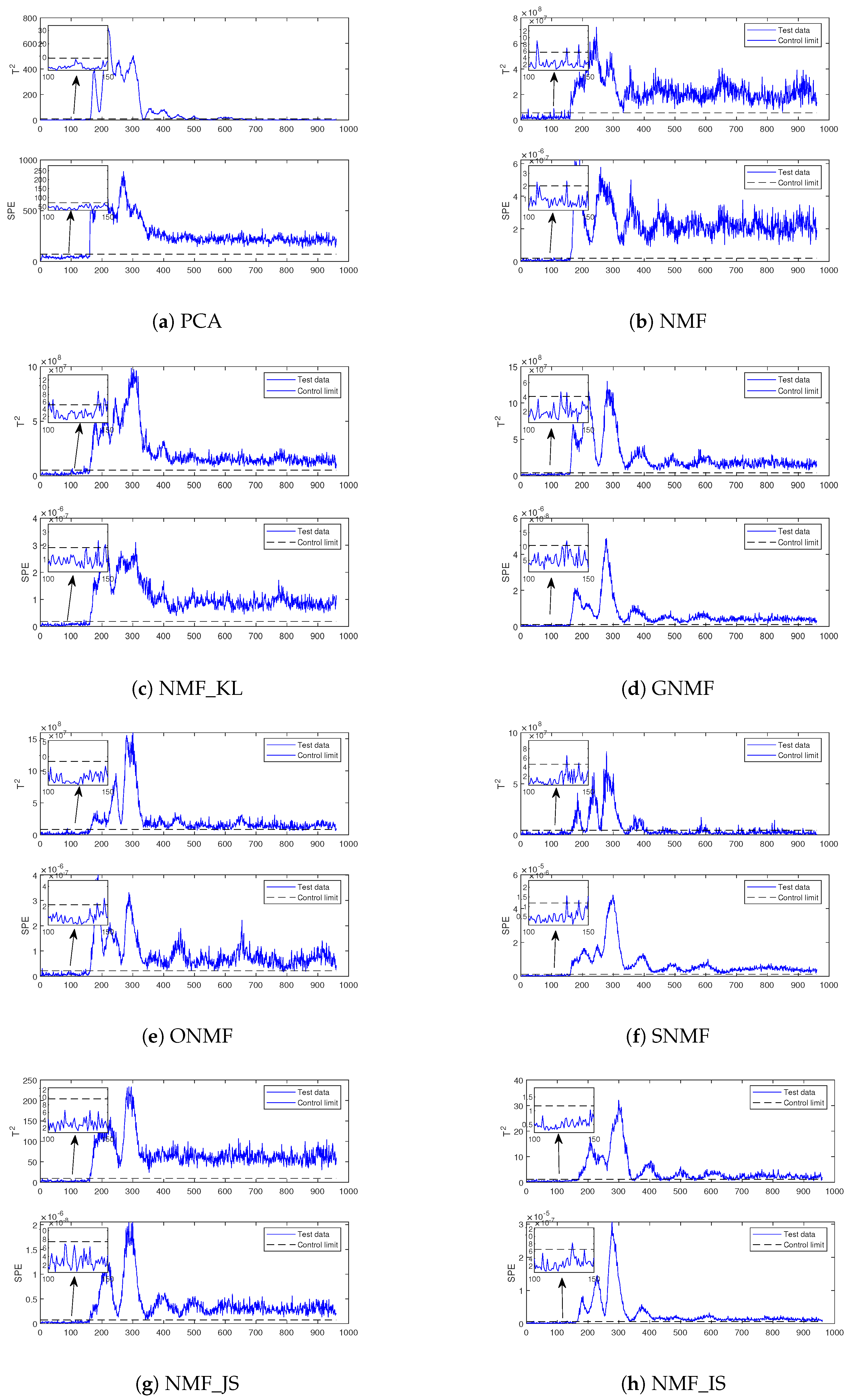
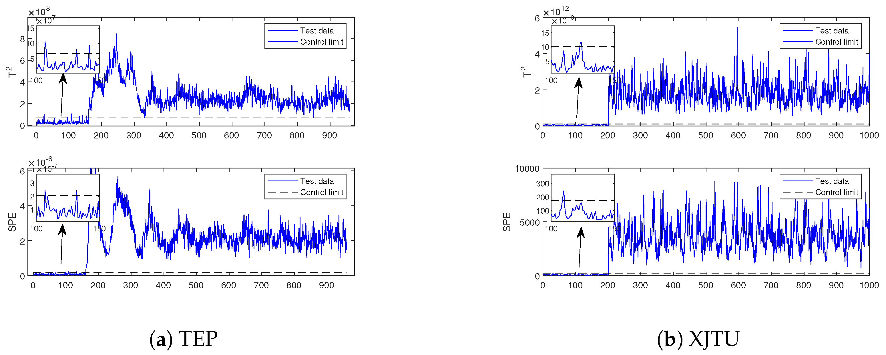
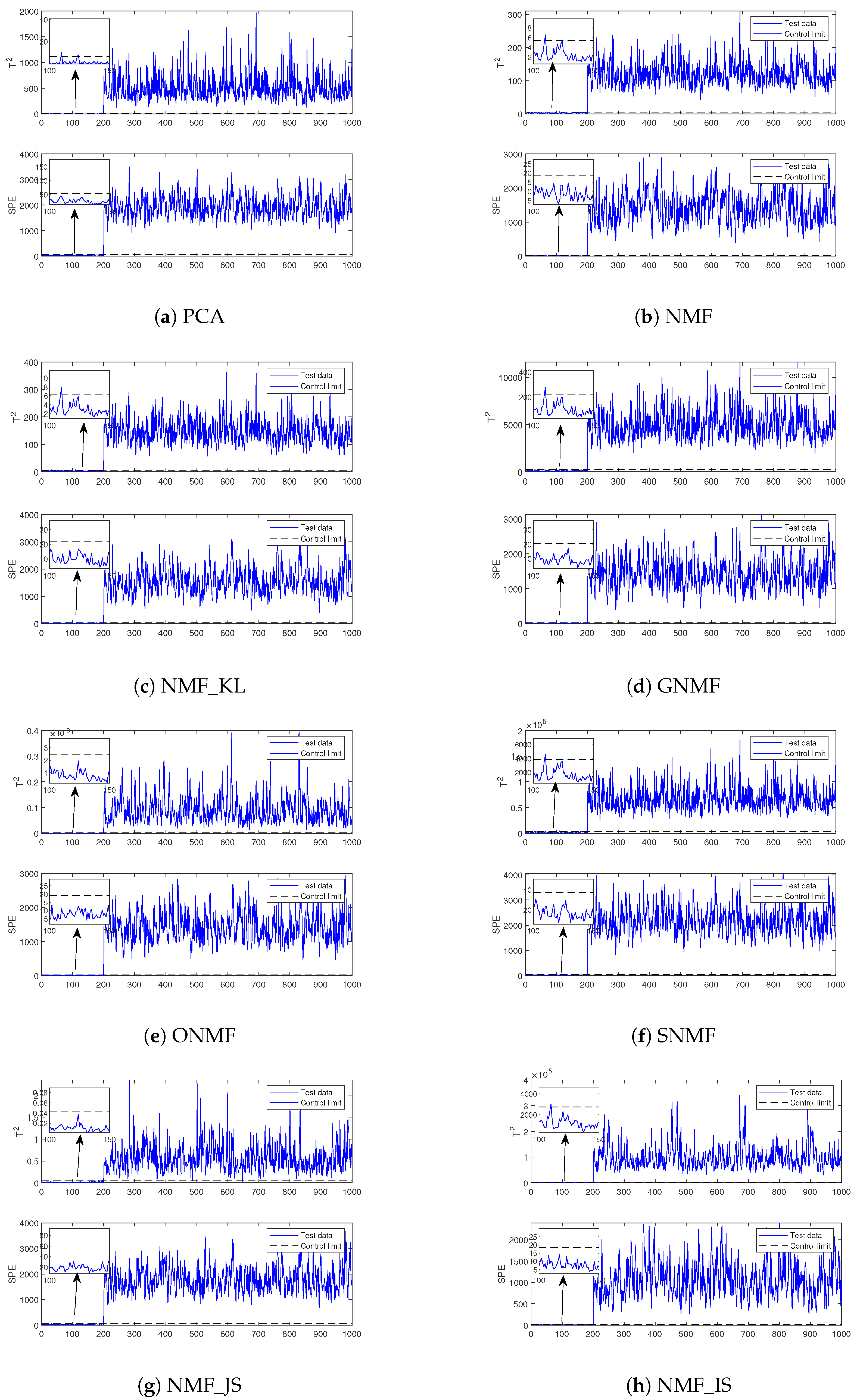
5.2.2. Results of the Experiment

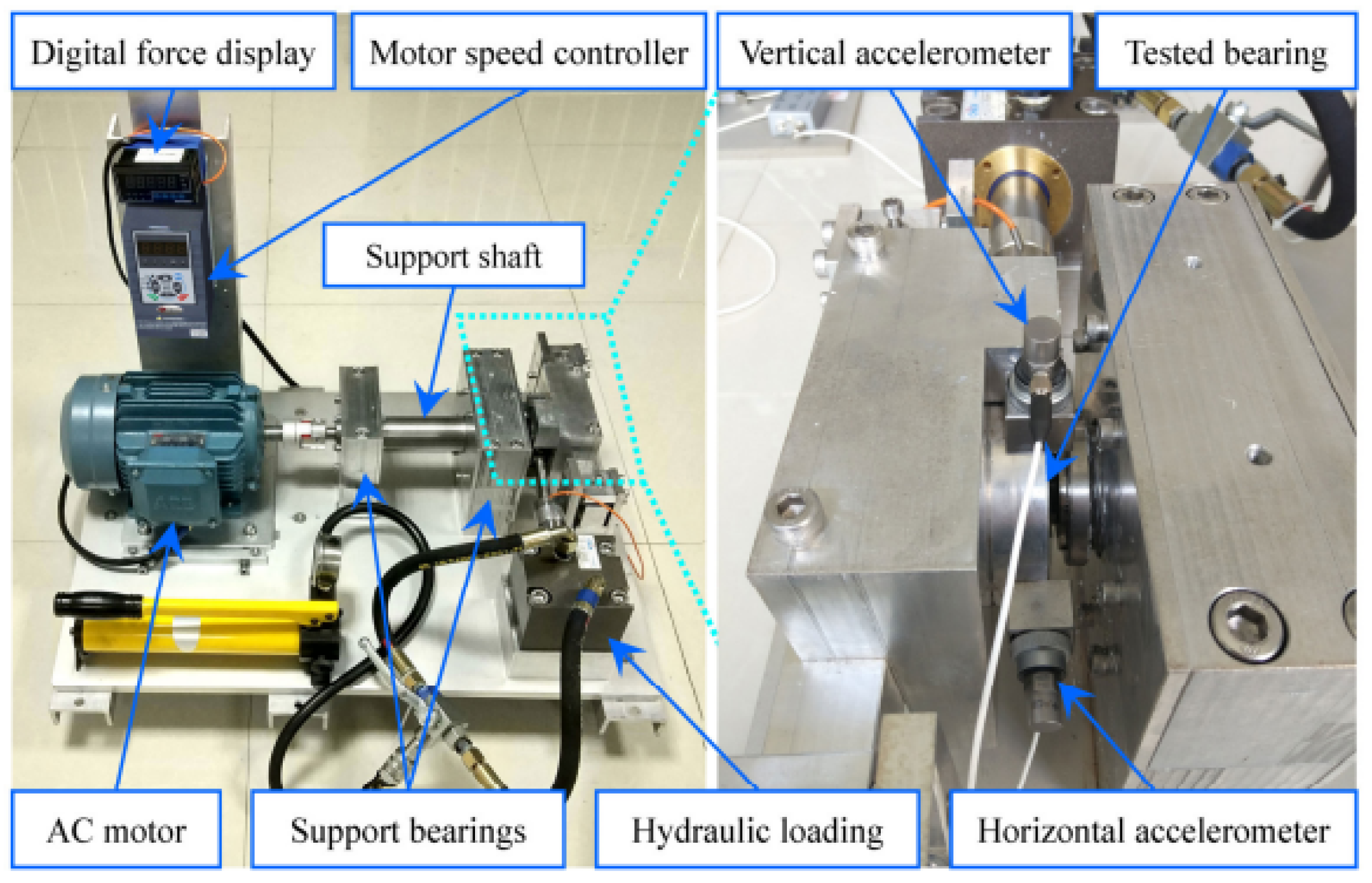
From

Table 1. FDR values for TEP.

	PCA		NMF		NMF_KL		NMF_IS		GNMF		ONMF		SNMF		NMF_JS		ISGONMF
	T2	SPE	T2	SPE	T2	SPE	T2	SPE	T2	SPE	T2	SPE	T2	SPE	T2	SPE	T2	SPE
IDV1	59.30	99.75	99.50	99.63	99.13	99.00	98.75	98.88	98.38	99.13	97.63	99.00	99.00	99.38	99.38	99.63	99.38	99.75
IDV2	30.38	98.63	97.75	97.61	97.75	98.00	97.13	98.50	97.50	98.00	96.75	97.38	97.50	98.75	97.75	98.13	98.00	96.63
IDV3	10.63	3.75	2.38	4.13	2.00	1.63	3.00	4.00	8.75	8.38	10.75	14.38	0.63	1.50	4.88	6.50	2.00	3.25
IDV4	6.00	93.88	11.38	52.13	2.25	2.63	1.38	6.63	3.13	5.50	1.25	5.38	0.75	5.25	12.88	32.38	15.75	47.00
IDV5	30.75	28.63	22.38	27.00	19.38	22.38	20.63	24.00	16.00	25.25	18.25	27.13	18.63	20.38	26.38	19.38	19.88	19.50
IDV6	99.38	99.38	99.88	99.88	100.00	100.00	100.00	100.00	99.25	100.00	98.50	100.00	100.00	99.88	99.50	98.50	99.63	99.63
IDV7	50.12	100.00	100.00	99.88	99.50	99.13	92.50	99.75	100.00	100.00	62.25	83.88	71.63	99.88	97.25	88.38	100.00	100.00
IDV8	89.00	97.50	93.63	97.33	88.50	91.13	90.75	92.38	70.50	92.25	68.75	90.13	72.13	92.88	87.38	64.88	94.75	87.00
IDV9	8.13	4.38	3.75	3.88	1.38	1.00	3.00	2.63	7.13	7.38	4.38	10.38	0.25	1.50	2.38	2.13	1.25	2.88
IDV10	52.75	42.75	31.13	38.63	26.63	30.88	28.88	29.38	31.38	43.88	37.13	47.88	12.65	18.33	15.50	13.13	13.50	23.25
IDV11	13.88	68.63	23.00	44.25	5.38	13.00	3.75	20.50	12.75	20.63	13.50	19.13	0.50	14.75	33.75	20.13	14.38	38.00
IDV12	92.13	98.63	88.63	95.38	81.00	82.25	81.75	84.38	68.38	88.38	69.13	86.25	77.83	89.38	75.88	56.38	79.00	90.38
IDV13	91.38	91.63	92.38	91.38	90.50	91.38	88.88	91.00	87.63	92.00	88.63	92.38	82.88	92.13	89.75	88.83	92.75	93.13
IDV14	19.50	88.38	56.63	81.88	6.88	48.38	3.63	57.13	5.63	29.75	3.00	11.75	5.13	62.63	62.00	52.00	34.38	97.63
IDV15	14.88	5.50	3.50	5.75	5.63	5.00	3.13	7.50	13.63	12.25	12.13	16.25	0.38	3.50	4.13	5.00	1.75	3.00
IDV16	38.75	27.13	51.75	61.63	29.88	30.38	22.63	20.50	33.25	47.38	43.75	55.63	25.13	53.38	57.13	20.63	60.50	63.75
IDV17	54.88	23.38	39.25	57.25	35.25	26.00	7.88	27.13	20.50	30.75	12.38	22.00	1.00	35.38	53.13	55.75	35.25	52.13
IDV18	88.38	90.00	88.73	98.13	88.38	87.88	88.50	89.25	83.13	87.63	81.38	86.63	84.88	88.88	87.63	95.63	81.13	92.25
IDV19	2.13	13.75	2.38	5.75	1.88	1.13	2.13	1.50	4.88	4.38	3.88	5.25	0.25	2.38	4.75	14.63	5.00	4.63
IDV20	21.38	28.88	21.88	42.13	12.88	20.50	11.00	22.13	23.25	29.25	18.38	35.63	13.25	20.38	63.75	64.38	40.88	47.75
IDV21	28.38	44.88	34.13	47.35	32.13	32.00	13.88	17.50	17.12	41.38	44.38	46.50	11.63	35.33	23.88	22.38	20.63	39.88
avreage	42.96	59.50	50.66	59.56	44.10	46.84	41.10	47.36	42.96	50.64	42.19	50.13	36.95	49.32	52.33	48.51	48.08	57.21

, we can see that the average value of the SPE index based on NMF is better than NMF_KL and NMF_IS. However, as can be seen from

Table 2. FAR values for TEP.

	PCA		NMF		NMF_KL		NMF_IS		GNMF		ONMF		SNMF		NMF_JS		ISGONMF
	T2	SPE	T2	SPE	T2	SPE	T2	SPE	T2	SPE	T2	SPE	T2	SPE	T2	SPE	T2	SPE
IDV1	0.00	2.50	0.00	0.00	0.00	0.00	1.25	0.00	0.00	0.00	0.00	0.00	0.63	0.00	1.88	0.00	0.00	2.50
IDV2	0.00	1.88	0.63	0.63	0.00	0.00	0.00	0.00	0.00	0.00	0.00	0.00	0.00	1.25	1.88	1.25	0.63	1.25
IDV3	6.38	1.25	2.50	2.50	0.00	0.00	0.63	0.63	0.63	0.00	0.00	1.25	0.00	0.63	3.75	5.63	0.63	1.88
IDV4	0.00	2.50	0.63	1.25	0.00	0.00	1.25	1.25	3.13	1.25	1.25	1.25	0.00	0.00	0.00	1.25	1.88	1.88
IDV5	0.00	2.50	0.63	1.25	0.00	0.00	1.25	1.25	3.13	1.25	1.25	1.25	0.00	0.00	4.21	1.88	1.25	0.63
IDV6	0.00	0.63	0.00	1.25	0.00	0.00	1.25	2.50	0.63	1.88	1.25	1.88	0.00	0.63	1.25	1.88	1.88	1.88
IDV7	0.63	0.00	2.50	4.38	0.00	0.00	0.63	1.25	1.25	0.63	6.88	11.88	0.00	0.63	0.00	1.25	4.38	1.25
IDV8	1.88	0.00	1.88	1.25	0.00	0.00	0.00	3.13	0.00	7.50	5.63	16.25	0.00	1.25	0.63	2.50	1.88	0.00
IDV9	24.38	1.88	8.78	7.63	0.00	0.00	2.50	5.63	15.63	21.25	17.38	18.73	1.25	0.63	5.63	1.88	0.63	3.13
IDV10	0.00	1.25	0.63	1.25	0.00	0.00	0.00	0.63	0.00	0.63	0.63	0.00	0.00	0.63	2.50	0.00	0.63	4.38
IDV11	0.00	3.13	0.63	3.13	0.00	0.00	0.00	1.88	6.88	0.00	2.50	2.50	0.00	1.25	1.25	5.00	1.25	1.88
IDV12	13.13	1.25	1.88	1.25	0.25	0.25	1.25	3.13	8.75	5.63	1.25	10.63	1.88	2.38	2.50	1.88	1.88	2.50
IDV13	0.00	0.00	0.00	0.63	0.00	0.00	0.00	1.25	0.00	0.00	0.00	0.00	0.00	0.00	0.00	2.50	1.25	0.63
IDV14	0.88	2.75	0.00	1.88	0.00	0.00	0.00	0.63	6.25	3.13	5.63	3.75	0.63	0.63	1.63	1.38	1.25	0.63
IDV15	0.00	1.25	0.63	0.63	0.00	0.00	1.25	0.00	0.63	0.00	0.00	1.25	0.63	1.25	2.50	1.88	1.25	3.13
IDV16	32.50	3.75	6.38	5.25	0.00	0.00	6.25	11.88	0.63	18.13	11.88	17.25	1.25	5.63	1.25	1.88	2.50	3.75
IDV17	0.00	1.88	1.25	4.38	0.00	0.00	1.88	2.50	10.13	7.25	13.13	16.25	1.25	1.25	1.25	2.50	4.38	1.88
IDV18	0.00	4.38	5.63	75.64	0.00	0.00	4.38	3.13	0.00	0.00	0.00	1.25	0.00	0.63	0.00	56.25	0.63	10.00
IDV19	0.00	0.00	0.63	1.88	0.00	0.00	1.25	1.88	3.75	2.50	0.63	3.13	0.00	1.25	0.63	0.63	1.25	0.00
IDV20	0.00	0.63	0.63	0.63	0.00	0.00	0.00	0.00	0.63	0.63	0.00	0.00	0.00	0.00	1.88	0.33	1.25	1.25
IDV21	2.50	3.13	0.63	0.63	0.00	0.00	1.88	1.88	0.00	0.63	0.00	0.63	0.25	1.38	1.88	0.63	1.25	1.25
avreage	3.91	1.73	1.73	5.58	0.01	0.01	1.28	2.11	2.95	3.60	3.29	5.19	0.36	1.01	1.74	4.40	1.59	2.17

, the average value of the FAR based on NMF is not as good as NMF_KL and NMF_IS, while the FDR based on NMF_IS is better than NMF_KL. This is the reason why we chose NMF based on IS divergence. And from Table 1, we can see that the average FDR of ISGONMF is superior to that of NMF_IS and most other traditional models based on NMF. Meanwhile, the analysis of the data indicates that ISGONMF performs exceptionally well in terms of FAR (false alarm rate). Across all tested Industrial Data Vectors (IDVs), ISGONMF achieves an average FAR value of $T^2$ being only 1.59%, as shown in Table 2, significantly lower than other methods. Notably, for IDVs such as IDV1, IDV8, and IDV19, the FAR of ISGONMF is close to zero, indicating virtually no false alarms. Moreover, compared to conventional methods, ISGONMF consistently maintains the lowest or near-lowest FAR across all IDVs, demonstrating its significant advantage in reducing false alarms. This makes ISGONMF highly effective in minimizing erroneous alerts and significantly enhancing system reliability in practical applications. Figure 3 shows the visualization of the eight compared algorithms in IDV7. Figure 4 shows the visualization of the model proposed in this paper on two datasets.

5.3. XJTU

The XJTU-SY dataset from Xi’an Jiaotong University offers valuable data on rolling bearings’ vibration and lifespan under various conditions [37]. It is mainly used for bearing-lifespan prediction and health monitoring research, supporting the development and assessment of machine learning and deep learning models [38,39]. The experimental setup, depicted in Figure 5, features an AC motor, speed controller, shaft, support bearing, hydraulic loading system, and test bearings. Data is gathered at 25.6 kHz using a portable dynamic signal acquisition unit, lasting 1 min and 28 s per sample. The CSV dataset includes vibration signals for analyzing different bearing fault types and characteristics.

5.3.1. Data Preparation

The study defined three distinct operational settings, each involving five bearings. Accelerometers attached to the bearings’ exterior captured vibration data at a rate of 25.6 kHz, with each session lasting 1.28 s. The data, including horizontal and vertical vibration measurements, were stored in CSV files. Testing continued until the peak vibration amplitude exceeded ten times that of normal operation, providing insight into the bearing’s deterioration from normal to critical failure. The dataset includes detailed information on the number of CSV files, operational lifespan, and failure types, such as inner race wear, cage rupture, outer race wear, and fracture. This dataset serves as valuable data for evaluating predictive maintenance algorithms for rolling element bearings, with the analysis focusing on the horizontal vibration data in the first column.

Table 3. FDR values for XJTU.

	PCA		NMF		NMF_KL		NMF_IS		GNMF		ONMF		SNMF		NMF_JS		ISGONMF
	T2	SPE	T2	SPE	T2	SPE	T2	SPE	T2	SPE	T2	SPE	T2	SPE	T2	SPE	T2	SPE
Bearing 1-1	95.60	95.48	95.11	95.47	95.24	95.60	95.11	95.48	95.24	95.60	95.36	95.36	94.88	95.48	95.24	95.48	95.36	95.24
Bearing 1-2	95.36	95.24	95.24	95.36	95.24	95.36	95.24	95.36	95.36	95.36	95.24	95.36	95.24	95.24	95.24	95.24	95.36	95.36
Bearing 1-3	95.24	95.24	95.24	95.48	95.24	95.24	95.36	95.48	95.24	95.36	95.24	95.36	95.36	95.24	95.24	95.36	95.24	95.36
Bearing 1-4	21.45	78.24	5.24	81.79	5.83	79.88	14.88	64.88	12.86	44.66	13.24	76.90	3.05	72.29	21.86	77.81	4.17	82.14
Bearing 1-5	5.00	13.46	4.41	23.13	4.51	19.89	5.83	14.29	4.38	16.48	3.24	16.76	3.33	8.14	5.00	27.19	7.86	4.76
Bearing 2-1	95.24	95.24	95.24	95.24	95.24	95.24	95.24	95.24	95.24	95.24	95.24	95.24	95.24	95.24	95.24	95.24	95.24	95.24
Bearing 2-2	95.24	95.24	95.24	95.24	95.24	95.24	95.24	95.24	95.24	95.24	95.24	95.24	95.24	95.24	95.24	95.24	95.24	95.36
Bearing 2-3	95.24	95.24	95.24	95.24	95.24	95.24	95.24	95.36	95.24	95.24	95.36	95.36	95.24	95.24	95.48	95.24	95.36	95.36
Bearing 2-4	3.36	15.48	14.12	33.36	7.71	32.62	10.71	17.62	5.98	28.95	3.52	25.52	2.19	35.81	12.96	16.09	2.86	6.07
Bearing 2-5	95.36	95.24	95.24	95.36	95.24	95.48	95.36	95.36	95.24	95.36	95.48	95.24	95.24	95.24	95.36	95.24	95.24	95.95
Bearing 3-1	95.24	95.24	95.24	95.48	95.24	95.24	95.24	95.24	95.24	95.24	95.36	95.24	95.36	95.36	95.24	95.36	95.24	95.24
Bearing 3-2	95.24	95.36	95.24	95.24	95.24	95.36	95.24	95.24	95.24	95.24	95.36	95.36	95.24	95.24	95.24	95.36	95.36	95.24
Bearing 3-3	95.48	95.24	95.47	95.36	95.48	95.36	95.48	95.24	95.48	95.48	95.24	95.60	95.36	95.36	95.24	95.48	95.36	95.48
Bearing 3-4	95.24	95.36	95.36	95.48	95.36	95.36	95.36	95.24	95.71	95.81	95.24	95.48	95.36	95.36	95.36	95.48	95.36	95.36
Bearing 3-5	29.05	95.24	31.67	95.48	28.34	95.12	71.79	95.24	28.57	95.48	77.38	95.38	11.67	95.81	75.33	95.81	32.22	95.56
avreage	73.82	83.37	73.55	85.51	72.95	85.07	76.76	82.71	73.35	82.31	76.38	84.22	71.20	84.02	77.55	84.37	73.03	82.51

of this study presents 15 different faults evaluated under three operational conditions. For each fault, the training dataset contains 1000 normal instances, while the test dataset consists of 200 normal instances and 800 fault instances.

5.3.2. Results of the Experiment

The ISGONMF algorithm exhibits significant strengths in the XJTU datasets. Regarding FDR, in terms of mean values, the ISGONMF algorithm has mean values of 77.55 and 84.37 for both T2 and SPE metrics, respectively, which indicates that the ISGONMF algorithm outperforms most of the other algorithms in terms of overall fault detection performance, in Table 3, Bearings 1-2, 1-4, 1-5, 2-1, 2-2, 2-5, and 3-3 showed better results. In terms of FAR, the ISGONMF algorithm achieved the lower average SPE value at just 0.96%, as shown in

Table 4. FAR values for XJTU.

	PCA		NMF		NMF_KL		NMF_IS		GNMF		ONMF		SNMF		NMF_JS		ISGONMF
	T2	SPE	T2	SPE	T2	SPE	T2	SPE	T2	SPE	T2	SPE	T2	SPE	T2	SPE	T2	SPE
Bearing 1-1	5.00	1.75	1.88	0.63	1.88	1.25	2.50	1.25	1.88	1.25	1.88	0.63	2.50	1.88	1.88	0.63	1.88	1.25
Bearing 1-2	1.88	1.25	0.00	2.50	0.00	3.13	0.63	1.88	0.00	2.50	1.25	3.75	0.00	1.88	0.63	3.13	1.88	1.25
Bearing 1-3	0.00	0.63	1.25	0.00	1.25	0.63	1.25	0.63	0.00	1.88	0.63	1.25	0.63	0.63	0.00	1.88	2.50	1.25
Bearing 1-4	0.62	0.62	1.87	1.87	1.88	2.50	1.25	2.50	1.25	1.25	1.25	1.25	1.88	3.13	1.88	0.63	1.25	3.13
Bearing 1-5	1.25	0.00	1.25	1.25	0.00	0.63	1.88	0.00	0.62	1.23	0.00	1.25	0.63	0.00	0.63	0.63	1.25	1.88
Bearing 2-1	0.00	0.63	0.63	0.63	0.63	0.00	0.63	0.63	0.63	1.25	0.63	0.63	0.63	1.25	1.25	1.88	0.00	1.88
Bearing 2-2	0.63	1.25	0.00	1.25	0.00	1.88	0.00	0.00	0.00	2.50	0.00	3.12	0.00	1.25	0.00	0.63	0.00	0.00
Bearing 2-3	0.00	3.13	1.88	0.00	1.88	0.00	0.63	0.63	0.00	0.00	0.63	0.00	1.86	0.00	1.25	1.25	1.25	0.63
Bearing 2-4	0.62	0.00	0.00	0.63	0.62	0.62	0.63	0.63	0.62	0.62	0.00	0.00	0.00	0.00	0.62	0.62	1.25	0.63
Bearing 2-5	0.63	0.00	1.25	0.00	1.25	0.00	0.63	0.63	1.25	1.25	0.63	0.63	1.25	0.00	0.63	1.88	0.63	0.63
Bearing 3-1	0.63	0.00	1.25	0.63	1.88	0.00	2.50	0.63	2.50	0.00	0.00	1.25	1.86	0.00	1.25	0.00	1.25	0.00
Bearing 3-2	1.25	1.25	3.13	2.50	2.50	1.25	2.50	0.63	1.88	1.88	0.00	0.63	1.86	0.63	2.50	2.50	1.88	0.63
Bearing 3-3	0.00	1.88	0.00	1.25	0.00	0.00	0.63	0.63	0.00	0.00	1.25	0.63	0.00	0.00	0.00	0.00	0.00	0.63
Bearing 3-4	1.25	0.00	0.62	0.62	0.63	0.63	0.63	0.63	0.63	0.63	1.25	0.63	0.63	1.25	0.63	0.00	0.00	0.63
Bearing 3-5	0.63	0.63	3.75	1.25	1.25	1.25	0.00	0.00	3.75	2.50	1.25	2.50	3.75	3.75	2.50	0.00	3.16	0.00
avreage	0.96	0.87	1.25	1.00	1.04	0.92	1.08	0.75	1.00	1.25	0.71	1.21	1.16	1.04	1.04	1.04	1.21	0.96

, indicating its effectiveness. On Bearings 2-2, 3-1, and 3-2, both T2 and SPE statistics are optimal, confirming that the algorithm maintains a considerably low false alarm rate across the bearing dataset. Figure 6 shows the visualization of the eight compared algorithms in Bearing2–5.

5.4. Ablation Study

Orthogonality constraints are essential to improve the performance of the model in fault detection tasks. As shown in the

Table 5. Ablation study results on TEP and XJTU-SY datasets.

Dataset	Model	FDR		FAR
		${\mathit{T}}^{\mathbf{2}}$(%)	SPE (%)	${\mathit{T}}^{\mathbf{2}}$(%)	SPE (%)
TEP	ISGONMF	48.08	57.21	1.59	2.17
	ISGNMF	46.63	52.13	1.71	2.35
XJTU-SY	ISGONMF	73.03	82.51	1.21	0.96
	ISGNMF	72.11	81.95	0.89	1.12

, we analyze the model performance on both TEP and XJTU-SY datasets in detail. In terms of fault detection rate (FDR), the orthogonality constraint enables the ISGONMF model to exhibit slightly higher performance than the ISGNMF model without the orthogonality constraint on both datasets, especially on the XJTU-SY dataset, where the ISGONMF model achieves an FDR $T^2$ of 73.03%, which is significantly higher than that of the ISGNMF model of 72.11%. This indicates that the orthogonality constraint helps the model to identify the faulty situations more effectively. In terms of false alarm rate (FAR), the orthogonality constraint also plays a significant role in improving it. On the TEP dataset, the FAR $T^2$ of the ISGONMF model is 1.59%, which is lower than the 1.71% of the ISGNMF model.

Summarizing the above analysis, we can conclude that the orthogonality constraint plays a crucial role in the ISGONMF model. It not only improves the fault detection rate of the model and reduces the false alarm rate, but also enhances the model’s ability to adapt to complex datasets. The orthogonality constraint helps the model to better capture the data features, thus improving the accuracy and reliability of fault detection.

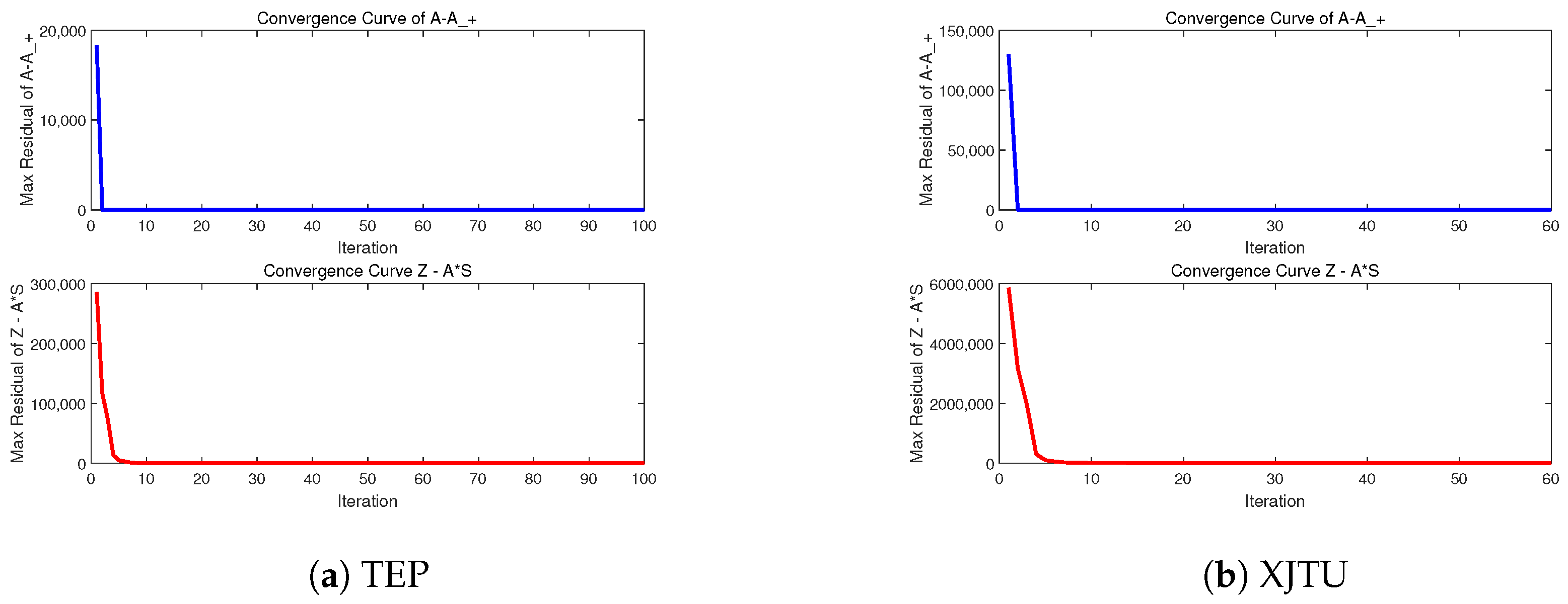
5.5. Experimental Convergence Results

Figure 7 demonstrates the convergence results of the algorithm on the datasets TEP and XJTU, the residuals ${\parallel Z-AS\parallel }_F$ and ${∥A-A_{+}∥}_F$ decrease rapidly within 20 iterations, indicating numerical stability. The algorithm terminates when $\parallel Z^k-A^k{S}^k{\parallel }_F<ϵ\left(ϵ={10}^{-5}\right)$ or reaches the maximum iterations (60). The convergence results of the TEP simulation experiments are shown in terms of IDV7, and the convergence results of the XJTU bearing dataset are shown in terms of bearings 2–5.

6. Conclusions

This study proposes a novel fault detection approach named Graph-Regularized Orthogonal Non-negative Matrix Factorization with Itakura–Saito (IS) Divergence (ISGONMF), specifically designed to address the challenges in complex industrial processes. By integrating graph regularization, orthogonal constraints, and the IS divergence, the method effectively captures the probabilistic characteristics of data and leverages the intrinsic relationships among data points to enhance the quality of matrix factorization. Experimental results demonstrate that ISGONMF achieves superior performance in reducing false alarm rates (FAR) and improving fault detection rates (FDR), particularly when applied to the Tennessee Eastman Process (TEP) dataset and the XJTU-SY dataset commonly used for bearing fault diagnosis. To further enhance the model’s adaptability and robustness, future work may explore the incorporation of additional divergence measures and the development of mechanisms for automatically selecting the most suitable divergence based on data characteristics. Moreover, efforts to improve model interpretability, visualization capabilities, and resilience against external disturbances will be key directions for further research.

References

1. Wang, Y.X.; Zhang, Y.J. Nonnegative matrix factorization: A comprehensive review. IEEE Trans. Knowl. Data Eng. 2012, 25, 1336–1353. [Google Scholar] [CrossRef]
2. Kim, H.; Park, H. Sparse non-negative matrix factorizations via alternating non-negativity-constrained least squares for microarray data analysis. Bioinformatics 2007, 23, 1495–1502. [Google Scholar] [CrossRef] [PubMed]
3. Lee, D.D.; Seung, H.S. Learning the parts of objects by non-negative matrix factorization. Nature 1999, 401, 788–791. [Google Scholar] [CrossRef]
4. Belachew, M.T. Efficient algorithm for sparse symmetric nonnegative matrix factorization. Pattern Recognit. Lett. 2019, 125, 735–741. [Google Scholar] [CrossRef]
5. Huang, S.; Wang, H.; Li, T.; Li, T.; Xu, Z. Robust graph regularized nonnegative matrix factorization for clustering. Data Min. Knowl. Discov. 2018, 32, 483–503. [Google Scholar] [CrossRef]
6. Yoo, J.; Choi, S. Orthogonal nonnegative matrix factorization: Multiplicative updates on Stiefel manifolds. In Proceedings of the International Conference on Intelligent Data Engineering and Automated Learning, Daejeon, Republic of Korea, 2–5 November 2008; Springer: Berlin/Heidelberg, Germany, 2008; pp. 140–147. [Google Scholar]
7. Cai, D.; He, X.; Han, J.; Huang, T.S. Graph regularized nonnegative matrix factorization for data representation. IEEE Trans. Pattern Anal. Mach. Intell. 2010, 33, 1548–1560. [Google Scholar] [CrossRef]
8. Berahmand, K.; Saberi-Movahed, F.; Sheikhpour, R.; Li, Y.; Jalili, M. A Comprehensive Survey on Spectral Clustering with Graph Structure Learning. arXiv 2025, arXiv:2501.13597. [Google Scholar]
9. Choi, S. Algorithms for orthogonal nonnegative matrix factorization. In Proceedings of the 2008 IEEE International Joint Conference on Neural Networks (IEEE World Congress on Computational Intelligence), Hong Kong, China, 1–8 June 2008; IEEE: Piscataway, NJ, USA, 2008; pp. 1828–1832. [Google Scholar]
10. Ding, C.; Li, T.; Peng, W.; Park, H. Orthogonal nonnegative matrix t-factorizations for clustering. In Proceedings of the 12th ACM SIGKDD International Conference on Knowledge Discovery and Data Mining, Philadelphia, PA, USA, 20–23 August 2006; pp. 126–135. [Google Scholar]
11. Saberi-Movahed, F.; Berahman, K.; Sheikhpour, R.; Li, Y.; Pan, S. Nonnegative matrix factorization in dimensionality reduction: A survey. arXiv 2024, arXiv:2405.03615. [Google Scholar] [CrossRef]
12. Chen, W.S.; Zeng, Q.; Pan, B. A survey of deep nonnegative matrix factorization. Neurocomputing 2022, 491, 305–320. [Google Scholar] [CrossRef]
13. Li, C.; Che, H.; Leung, M.F.; Liu, C.; Yan, Z. Robust multi-view non-negative matrix factorization with adaptive graph and diversity constraints. Inf. Sci. 2023, 634, 587–607. [Google Scholar] [CrossRef]
14. Zhang, W.; Yu, S.; Wang, L.; Guo, W.; Leung, M.F. Constrained symmetric non-negative matrix factorization with deep autoencoders for community detection. Mathematics 2024, 12, 1554. [Google Scholar] [CrossRef]
15. Dong, Y.; Che, H.; Leung, M.F.; Liu, C.; Yan, Z. Centric graph regularized log-norm sparse non-negative matrix factorization for multi-view clustering. Signal Process. 2024, 217, 109341. [Google Scholar] [CrossRef]
16. Yang, X.; Che, H.; Leung, M.F.; Liu, C. Adaptive graph nonnegative matrix factorization with the self-paced regularization. Appl. Intell. 2023, 53, 15818–15835. [Google Scholar] [CrossRef]
17. Li, X.b.; Yang, Y.p.; Zhang, W.d. Fault detection method for non-Gaussian processes based on non-negative matrix factorization. Asia-Pac. J. Chem. Eng. 2013, 8, 362–370. [Google Scholar] [CrossRef]
18. Xiao, L.; Yang, X.; Yang, X. A graph neural network-based bearing fault detection method. Sci. Rep. 2023, 13, 5286. [Google Scholar] [CrossRef]
19. Ren, Z.; Zhang, W.; Zhang, Z. A deep nonnegative matrix factorization approach via autoencoder for nonlinear fault detection. IEEE Trans. Ind. Inform. 2019, 16, 5042–5052. [Google Scholar] [CrossRef]
20. Xiu, X.; Fan, J.; Yang, Y.; Liu, W. Fault detection using structured joint sparse nonnegative matrix factorization. IEEE Trans. Instrum. Meas. 2021, 70, 3513011. [Google Scholar] [CrossRef]
21. Zhang, X.; Xiu, X.; Zhang, C. Structured joint sparse orthogonal nonnegative matrix factorization for fault detection. IEEE Trans. Instrum. Meas. 2023, 72, 2506015. [Google Scholar] [CrossRef]
22. Ahmadian, S.; Berahmand, K.; Rostami, M.; Forouzandeh, S.; Moradi, P.; Jalili, M. Recommender Systems based on Non-negative Matrix Factorization: A Survey. IEEE Trans. Artif. Intell. 2025, 1–21. [Google Scholar] [CrossRef]
23. Févotte, C.; Bertin, N.; Durrieu, J.L. Nonnegative matrix factorization with the Itakura-Saito divergence: With application to music analysis. Neural Comput. 2009, 21, 793–830. [Google Scholar] [CrossRef]
24. Cichocki, A.; Lee, H.; Kim, Y.D.; Choi, S. Non-negative matrix factorization with α-divergence. Pattern Recognit. Lett. 2008, 29, 1433–1440. [Google Scholar] [CrossRef]
25. Févotte, C.; Idier, J. Algorithms for nonnegative matrix factorization with the β-divergence. Neural Comput. 2011, 23, 2421–2456. [Google Scholar] [CrossRef]
26. Yang, Z.; Zhang, H.; Yuan, Z.; Oja, E. Kullback-Leibler divergence for nonnegative matrix factorization. In Proceedings of the International Conference on Artificial Neural Networks, Espoo, Finland, 14–17 June 2011; Springer: Berlin/Heidelberg, Germany, 2011; pp. 250–257. [Google Scholar]
27. Hien, L.T.K.; Gillis, N. Algorithms for nonnegative matrix factorization with the Kullback–Leibler divergence. J. Sci. Comput. 2021, 87, 93. [Google Scholar] [CrossRef]
28. Zhang, L.; Liu, Z.; Pu, J.; Song, B. Adaptive graph regularized nonnegative matrix factorization for data representation. Appl. Intell. 2020, 50, 438–447. [Google Scholar] [CrossRef]
29. Chen, K.; Che, H.; Li, X.; Leung, M.F. Graph non-negative matrix factorization with alternative smoothed L 0 regularizations. Neural Comput. Appl. 2023, 35, 9995–10009. [Google Scholar] [CrossRef]
30. Zhang, G.; Wang, Y.; Lessard, L.; Grosse, R.B. Near-optimal local convergence of alternating gradient descent-ascent for minimax optimization. In Proceedings of the International Conference on Artificial Intelligence and Statistics—Proceedings of Machine Learning Research, Virtual, 28–30 March 2022; pp. 7659–7679. [Google Scholar]
31. Harper, J.; Wells, D. Recent advances and future developments in PGD. Prenat. Diagn. 1999, 19, 1193–1199. [Google Scholar] [CrossRef]
32. Hajinezhad, D.; Chang, T.H.; Wang, X.; Shi, Q.; Hong, M. Nonnegative matrix factorization using ADMM: Algorithm and convergence analysis. In Proceedings of the 2016 IEEE International Conference on Acoustics, Speech and Signal Processing (ICASSP), Shanghai, China, 20–25 March 2016; IEEE: Piscataway, NJ, USA, 2016; pp. 4742–4746. [Google Scholar]
33. Lin, C.J. Projected gradient methods for nonnegative matrix factorization. Neural Comput. 2007, 19, 2756–2779. [Google Scholar] [CrossRef]
34. Yin, S.; Ding, S.X.; Haghani, A.; Hao, H.; Zhang, P. A comparison study of basic data-driven fault diagnosis and process monitoring methods on the benchmark Tennessee Eastman process. J. Process Control 2012, 22, 1567–1581. [Google Scholar] [CrossRef]
35. Lee, G.; Han, C.; Yoon, E.S. Multiple-fault diagnosis of the Tennessee Eastman process based on system decomposition and dynamic PLS. Ind. Eng. Chem. Res. 2004, 43, 8037–8048. [Google Scholar] [CrossRef]
36. Zhang, C.; Guo, Q.; Li, Y. Fault detection in the Tennessee Eastman benchmark process using principal component difference based on k-nearest neighbors. IEEE Access 2020, 8, 49999–50009. [Google Scholar] [CrossRef]
37. Wang, B.; Lei, Y.; Li, N. XJTU-SY bearing datasets. Github Github Repos. 2018. [Google Scholar]
38. Wang, B.; Lei, Y.; Li, N.; Li, N. A hybrid prognostics approach for estimating remaining useful life of rolling element bearings. IEEE Trans. Reliab. 2018, 69, 401–412. [Google Scholar] [CrossRef]
39. Xue, Y.; Yang, R.; Chen, X.; Tian, Z.; Wang, Z. A novel local binary temporal convolutional neural network for bearing fault diagnosis. IEEE Trans. Instrum. Meas. 2023, 72, 3525013. [Google Scholar] [CrossRef]
Figure 1. The framework diagram of Graph-Regularized Orthogonal Non-negative Matrix Factorization with Itakura–Saito (IS) Divergence. The top left of the image shows the classical NMF model, the bottom left shows the added regularization and constraint terms, and the right side of the image shows the fault detection process, which detects whether a fault has occurred based on the fault collection samples.
Mathematics 13 02343 g001
Figure 2. NMF-based fault detection process.
Mathematics 13 02343 g002
Figure 3. Detection results of fault IDV7 for TEP datasets.
Mathematics 13 02343 g003
Figure 4. Detectionresults for ISGONMF on two datasets.
Mathematics 13 02343 g004
Figure 5. XJTU-SY bearing dataset experiment platform.
Mathematics 13 02343 g005
Figure 6. Detection results of Bearing 2–5 for XJTU datasets.
Mathematics 13 02343 g006
Figure 7. Convergence results.
Mathematics 13 02343 g007