Abstract
This article concerns a Cournot duopoly game with homogeneous expectations. The cost functions of the two players are assumed to be asymmetric to capture possible asymmetries in firms’ technologies or firms’ input costs. Large values of the speed of adjustment of the players destabilize the Nash Equilibrium (N.E.) and cause the appearance of a chaotic trajectory in the Discrete Dynamical System (D.D.S.). The scope of this article is to control the chaotic dynamics that appear outside the stability field, assuming asymmetric cost functions of the two players. Specifically, one player uses linear costs, while the other uses nonlinear costs (quadratic or cubic). The cubic cost functions are widely used in the Economic Dispatch Problem. The delayed feedback control method is applied by introducing a new control parameter at the D.D.S. It is shown that larger values of the control parameter keep the N.E. locally asymptotically stable even for higher values of the speed of adjustment.
Keywords:
Cournot duopoly game; discrete dynamical system; bifurcation diagram; chaotic attractor; Lyapunov numbers; complexity; chaotic behavior; delayed feedback control; chaos control; cubic cost function; non-convex cost function MSC:
91B; 91A; 34H; 37N40
JEL Classification:
C02; C6; C7
1. Introduction
A market structure between monopoly and perfect competition, and a small number of companies participates is named oligopoly. Despite the small number of firms in an oligopoly, its operation is not that simple as the companies participating in it must assume not only consumer preferences but also make estimates regarding the decisions of their rivals. Augustin Cournot first formulated the theory of the oligopoly in 1838 [1] and studied the case of naïve players (firms), who decide at each time considering the decisions of the opponents of the previous period without appreciating future periods.
The players (firms) participating in an oligopoly model adjust their decisions towards the profit-maximizing amount using their expectations’ strategy. Duopolies with homogeneous expectations were considered by some authors [2,3,4,5,6,7,8,9,10] and complex dynamics are found in their games, such as chaotic attractors. Also, heterogeneous expectations were studied by other authors [11,12,13,14,15,16,17,18]. However, the producers have no knowledge of the entire market in real markets, but it is possible for them to have a perfect knowledge of production technology, which the cost function represents. For this reason, it is more likely that players employ some local estimate of the marginal profits. This case has been studied in articles [19,20,21,22,23,24,25]. Firms update their production estimate based on discrete time periods, behaving as bounded rational players and using a local estimate of the marginal profit. Therefore, following this adjustment mechanism, they are not requested to have a complete knowledge of the market and the cost functions [11,12,23,26]. More recent studies [27,28] have shown particular interest in replacing profit maximizations with relative profit maximization.
The authors of [29] investigate the case of bounded rational players that produce differentiated products under cost functions’ asymmetry (linear for player 1 and quadratic for player 2). In this duopoly model, each player (firm) is interested in maximizing an objective function that contains a percentage of their own profits and the remaining percentage of their opponent’s profits. Among other parameters, the effect of the parameter that expresses the speed of adjustment (parameter k) on the N.E.’s local stability was studied and it was found that large values of this parameter cause destabilization of the economy and from a value above this, they create chaotic trajectories in the D.D.S., something that is highlighted by chaotic attractors that make their appearance, by Lyapunov numbers that exceed unity and by the system’s sensitivity on its initial conditions that arises.
Many authors, such as Agiza [2], Du et al. [30], Holyst and Urbanowicz [31], Ding et al. [32], Elabbasy et al. [33] and Pu and Ma [34], have considered methods to control the chaotic behavior on their studies. The central idea of this article is the application of the delayed feedback control method [35,36,37,38] to this duopoly game with asymmetric cost functions in order to control the chaos that appears when the parameter of the speed of adjustment takes values outside the local stability field. The novelty of the present work in relation to [35] is that the method is applied to a duopoly where the players use different production technologies (asymmetric costs). The asymmetric cost functions can capture the possible asymmetries in firms’ technologies or firms’ input costs. For example, one firm may have a technological advantage or better access to raw materials, leading to lower marginal costs. In reality, firms rarely have identical cost functions. As a result, our assumption of asymmetric cost functions can capture the inherent heterogeneity of the firms [39,40]. In addition, this asymmetry creates even greater complexity in the D.D.S. of the game.
The authors present a modified game where the second player uses the cubic cost function. The cubic cost function is widely used in studies over the energy sector. The results are similar to those of the quadratic cost case, i.e., large values of the speed of adjustment (parameter k) destabilize the N.E. and from a certain value and above, the system starts to behave chaotically and in an unpredictable way. Furthermore, it was observed that with cubic cost function and as the values of the parameter k increase, the instability in the N.E. and the period doubling bifurcations start from smaller values of parameter k. Finally, the delayed feedback control method is successfully applied in this modified game with cubic cost function and manages to control the chaotic behavior of the system, which happens when the parameter k takes values outside the stability space.
2. The Original Game with Quadratic Cost Function
In [27], a Cournot-type duopoly game with differentiated products was studied, where the players use asymmetric cost functions and follow homogenous strategies (bounded rational players). They were based on the following inverse demand functions:
As previously mentioned, the players use different cost functions. Specifically, player 1 uses a linear cost function:
while player 2 uses a quadratic cost function:
With the above assumptions, the players have the following profit functions:
and
According to the original article, each i-player is interested in maximizing an objective function, which consists of a percentage of the difference in the profits of the two players and by from their own profits describing as follows:
The economic reason why the relative profit function takes into account the profits of both players (player i and player j) is clarified through two representative examples:
- (i)
- The management (decision-making) can be distinguished from the ownership. This means that the one who makes decisions on production quantities (Cournot, not Bertrand) may not be trustworthy and therefore may be bribed for an advantage over the opponent.
- (ii)
- The owner of a company (player i) also participates in the opponent company (player j) [41].
The partial derivatives of are described by the following equations:
and
The authors seek a mechanism that could lead the economy (the oligopolistic market) to N.E. This mechanism can be a D.D.S. with the same N.E. of static game. For this purpose, the authors use the marginal relative profit function instead of the simple marginal profit , following the strategy of bounded rationality for both players. This means that each firm i is described as a bounded rational player and decides their production quantity for every discrete time period following the following mechanism:
where k is the positive (k > 0) speed of adjustment of the two players. Through this mechanism, each i-player decides to increase their level of adaptation when their marginal objective function is positive and decreases their level of adaptation when it is negative. The D.D.S. of this duopoly is described as follows:
Searching for the conditions under which the N.E. is locally asymptotically stable, the proposition of the original game gives the following local stability conditions:
and
Through some numerical simulations for specific values of the exogenous variables of the game, it was revealed that large values of parameter k may destabilize the economy and create chaotic trajectories for the D.D.S. Also, this chaotic behavior of the system is revealed through the sensitivity of its initial conditions, and it is shown that outside the local stability range for parameter k, only a small change in the initial conditions can bring about enormous differences in the subsequent evolution of the system.
3. Chaos Control of the Original Game
3.1. Application of the Delayed Feedback Control Method to the Original Game
In this subsection, the authors apply the delayed feedback method to reduce the effect of the speed of adjustment and consequently control the chaotic dynamics that develop when parameter k takes values outside the local stability field. We employ the delayed feedback control method [35]. However, the key difference in comparison with [35] is that, in the present work, the cost functions of the two bounded rational players are assumed to be asymmetric, i.e., the two players use different production technologies. The delayed feedback control method is applied by introducing a new control parameter, m. Through this control method, a control signal is added to each difference equation of the D.D.S. of Equation (10), which is calculated as follows:
where and .
Appling the previous control signal setting gives a positive multiple of the difference between productions of two consecutive time periods t and t + 1:
For each i-player, the production quantity for the time period t + 1 becomes as follows:
and the new D.D.S. becomes as follows:
In this D.D.S. of Equation (16), it is studied whether its chaotic behavior can be controlled by the new control parameter that appears for values outside the local stability region chosen for parameter k, e.g., k = 0.58.
Setting:
and the D.D.S. of Equation (16) becomes as follows:
Determining a critical value of:
for which the N.E. may lose its local stability, and solving Equation (18) for m yields:
From a mathematical point of view, the above relationship shows that parameters k and m are related to each other in an increasing linear relationship. This means that larger values of parameter k and larger values of control parameter m are required in order to control chaos.
3.2. The Nash Equilibrium and Local Stability of the Original Game Under the Control Parameter
The new D.D.S. of Equation (16) has the same N.E. with the original one, which is as follows:
and its coordinates are not affected by control parameter m. Also, from the coordinates of N.E. position, the following equations arise:
The local stability of the N.E. can be studied using the Jacobian matrix of the D.D.S. of Equation (16) and it is given by the following matrix:
and substituting the coordinate values of the N.E. position on it, it takes the following form:
with trace:
and determinant:
Proposition 1.
The N.E. position of the D.D.S. of Equation (16) is locally asymptotically stable if:
and
Proof.
The N.E. position is locally asymptotically stable if the following three inequalities are simultaneously satisfied [42]:
The first Equation (i) becomes as follows:
which is the first condition of the local stability.
The second Equation (ii) becomes as follows:
that is always satisfied because of Equation (24).
The third Equation (iii) gives:
and this is the second condition of the local stability. □
3.3. Numerical Simulations of the Original Game Under the Control Parameter
This subsection presents some numerical simulations to show the local stability region focusing on control parameter m, to plot the N.E. equilibrium position, and to reveal the chaotic behavior and the sensitivity dependence on the initial conditions of the system in Equation (16) when the control parameter takes values outside its local stability space. It is necessary to set specific values to the exogenous variables: α = 5, c = 1, d = 0.50, μ = 0.70.
These specific values of exogenous variables α, c, d and μ, give the coordinates of the N.E. as follows:
Also, the value of k = 0.58 is chosen for the speed of adjustment, a value that causes chaos according to the original article. With these assumptions, the local stability interval results from the common solutions of Equations (29) and (30) and it is described as follows:
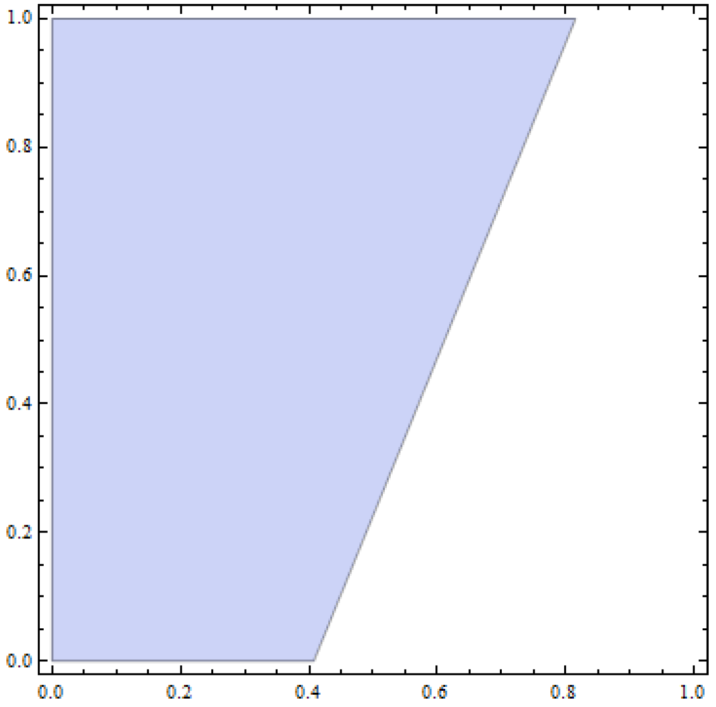
In Figure 1, it can be seen that the value of 0.58 for parameter k creates the local stability interval of Equation (33). A very important result is with larger values of control parameter m, the larger values of the speed of adjustment do not cause chaotic trajectories in the D.D.S.

Figure 1.
Stability region of Equations (29) and (30) between parameters k, speed of adjustment (horizontal axis), and m, control parameter (vertical axis), for α = 5, c = 1, d = 0.50 and μ = 0.70.
In Figure 2a,b the bifurcation diagrams of the production quantities q1 and q2 with respect to the control parameter m (horizontal axis) are presented. In these figures, it can be seen that for values of the speed of adjustment that cause chaotic trajectories, e.g., k = 0.58, the control parameter m can make the N.E. remain locally asymptotically stable. On the other hand, smaller values of the parameter m can make the system lose its local stability through period-doubling bifurcation, and for very small values, it can make it behave chaotically. For these specific values of parameters α, c, d, μ and k that were chosen by the authors, the common solution of Equation (29), , and Equation (30), , is the interval . The first values of parameter m < 0.41 violate the stability condition of 1 + Tr (J) + Det (J) > 0, but allow the condition of 1—Det (J) > 0 to continue to hold. That is why the route to chaos is through period-doubling bifurcations.
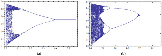
Figure 2.
Bifurcation diagrams with respect to the control parameter m (horizontal axis) with 400 iterations of the map of Equation (16) for : (a) against variable ; (b) against variable .
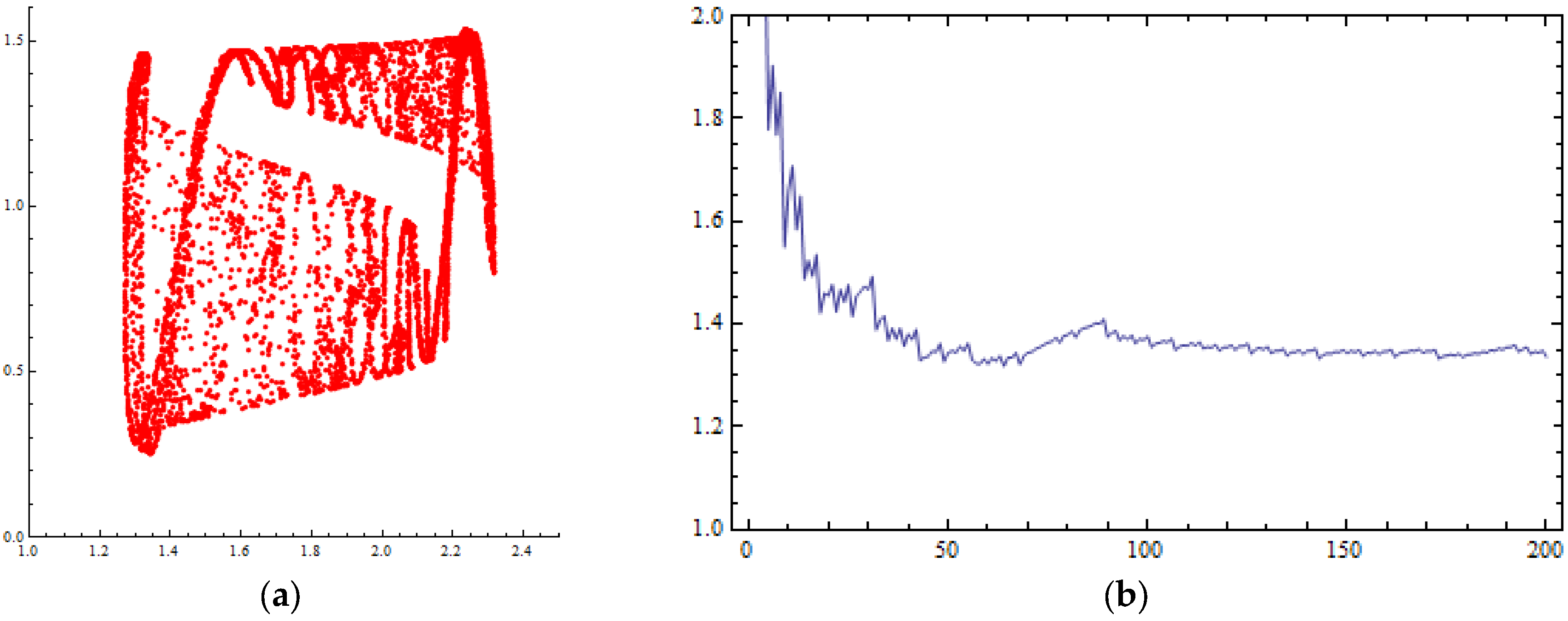
Figure 3a presents the chaotic attractor that can be created for small values of the control parameter m (e.g.,) as evidence of the chaotic behavior of the D.D.S. of Equation (16). Small values of parameter m make the delayed feedback method inefficient in controlling the system’s chaotic behavior. Another sign of the chaotic trajectory is the Lyapunov numbers that were calculated to be greater than 1 for (outside the stability interval of m). This graph is presented in Figure 3b.
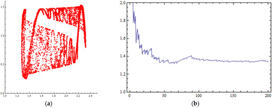
Figure 3.
Numerical simulations of the orbit of (0.1, 0.1) of the map of Equation (16) for : (a) phase portrait (chaotic attractor) with 8000 iterations; (b) Lyapunov numbers’ graph.
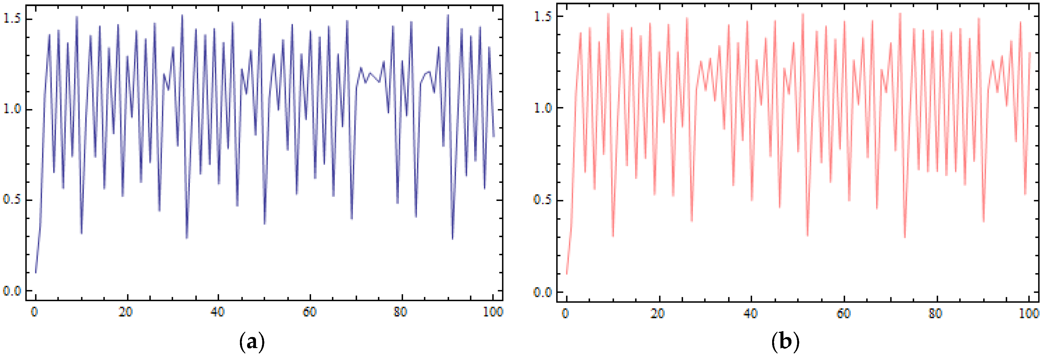
Finally, in Figure 4a,b, the time series of coordinate q1 are presented for two different initial conditions, (0.1, 0.1) (Figure 4a) and (0.101, 0.1) (Figure 4b), choosing the value of m = 0.02. At the beginning, the time series seem to be identical, but for a number of iterations later, the differences between them build up rapidly. For small values of the control parameter m, the D.D.S. of Equation (16) becomes sensitive in its initial conditions’ selection. Small changes on the first coordinate of the initial conditions can cause a completely different trajectory for the D.D.S. of Equation (16).
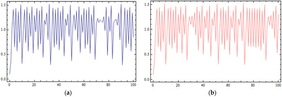
Figure 4.
Sensitive dependence on initial conditions for q1 coordinate plotted against the time of the system of Equation (16) for (a) The orbit of (0.1, 0.1); (b) the orbit of (0.101, 0.1).
4. A Modified Game with Cubic Cost Function
4.1. The Modified Game with Cubic Cost Function
We study a modified version of the original game which was presented in Section 2. We assume now that the cost function of the second player is cubic. This assumption is used in the Energy Sector. Specifically, in load distribution problems among multiple generation units, with the aim of minimizing the total cost of electricity generation, under demand and unit capacity constraints. This is known as the Economic Dispatch Problem [43,44,45,46]. The reasons why the scientific community uses the cubic cost function in such problems are the following: (a) the nonlinear behavior of fuel, (b) the technical limitations of units (operation characteristics)—higher-order polynomials better approximate real functions and give a more accurate modeling of these; and (c) because it reflects non-convexity, allowing us to model non-convex regions, which is necessary in unit commitment problems, security-constrained dispatch and real-time pricing optimization.
For this modified game, the same Equations (1) and (2) and a cubic cost function for the second player are considered with:
where is the non-negative fixed production cost.
Suppose that the marginal cost has a minimum point for
This means that:
(a)
The minimum is a non-negative quantity which gives
(b) which gives
In addition, it must be which gives
In total, the following restrictions apply to the cubic cost function:
The cubic cost function changes the profit function of the second player, which becomes as follows:
From the profit function of the second player, the following partial derivatives are calculated:
Using the objective function of Equation (6), it is found that the partial derivative of function remains the same as that of Equation (7) and the partial derivative of new function is described as follows:
4.2. The Nash Equilibrium and Local Stability of the Modified Game
The discrete dynamical system applied in this modified game is the same as in Equation (10):
and it gives the coordinates of the N.E. are calculated as the non-negative solutions of the following algebraic system:
The following proposition describes the local stability conditions for the N.E.
Proposition 2.
The N.E. position of the D.D.S. of Equation (38) is locally asymptotically stable if:
and
Proof.
The Jacobian matrix of the D.D.S. of Equation (38) is the following:
with trace:
and determinant:
The N.E. position is locally asymptotically stable if the three conditions of Equation (31) are simultaneously satisfied [42].
The first condition (i) gives:
that is the first local stability condition of the N.E.
The second condition (ii) becomes:
an inequality that is always satisfied.
The third condition (iii) gives:
which is the second local stability condition. □
4.3. Numerical Simulations of the Modified Game
In this subsection, some numerical simulations are presented to visualize the algebraic results of Proposition 2. For this reason, specific values for the game’s parameters are selected. Specifically, . Using these parameters’ values for the D.D.S. of Equation (38) and solving the algebraic system of Equation (39) it is found that there is a unique N.E. with coordinates:
Also, the common solutions of the local stability conditions of Equations (39) and (40) focusing on the parameter k are as follows:
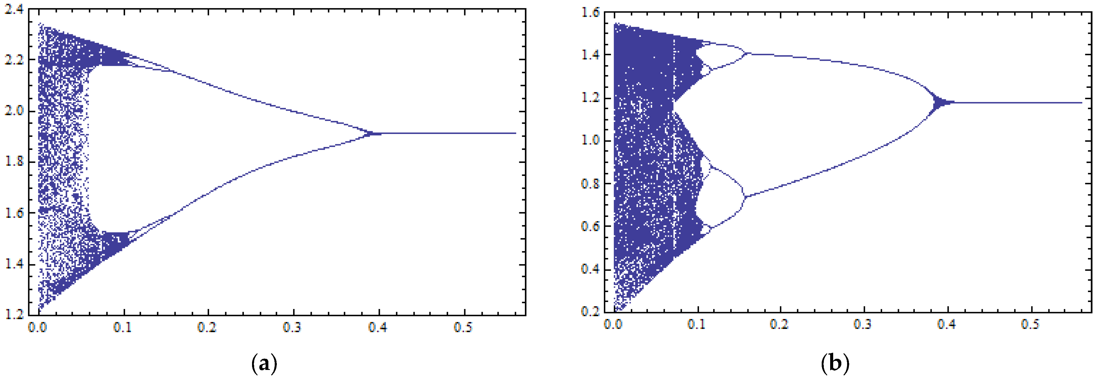
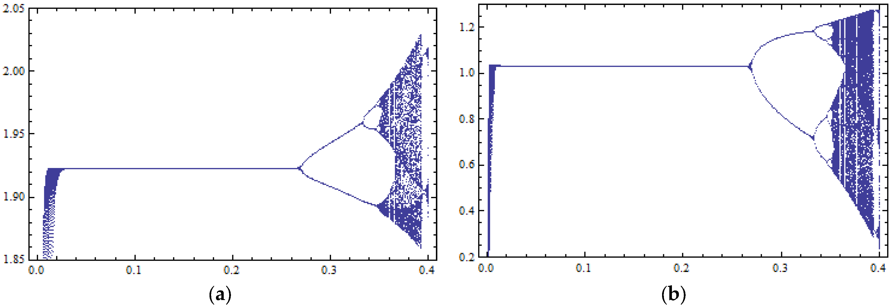
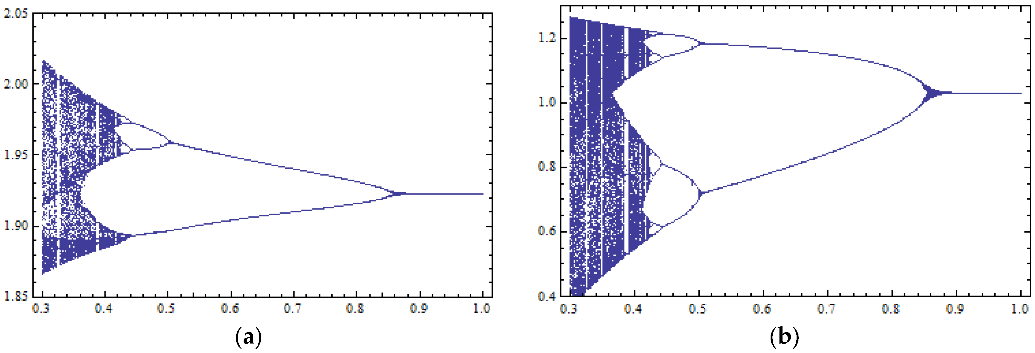
This result is verified by the bifurcation diagrams of (Figure 5a) and (Figure 5b) with respect to parameter k. It seems there is an N.E. with coordinates (1.92, 1.03), which is locally asymptotically stable when parameter k takes values lower than 0.27. After these values, as parameter k takes larger values, the N.E. loses its local stability through period-doubling bifurcations.
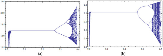
Figure 5.
Bifurcation diagrams with respect to the control parameter k (horizontal axis) with 400 iterations of the map of Equation (38) for : (a) against variable ; (b) against variable .
In this case of the cubic cost function for the second player, high values of parameter k cause chaotic behavior for the D.D.S. of Equation (38), and as evidence of this chaotic orbit, chaotic attractors and Lyapunov numbers larger than 1 appear. The chaotic attractor and Lyapunov numbers are presented in Figure 6a,b, respectively, for .
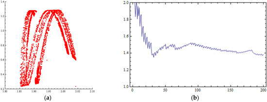
Figure 6.
Numerical simulations of the orbit of (0.1, 0.1) of the map of Equation (16) for . (a) Phase portrait (chaotic attractor) with 8000 iterations; (b) Lyapunov numbers’ graph.
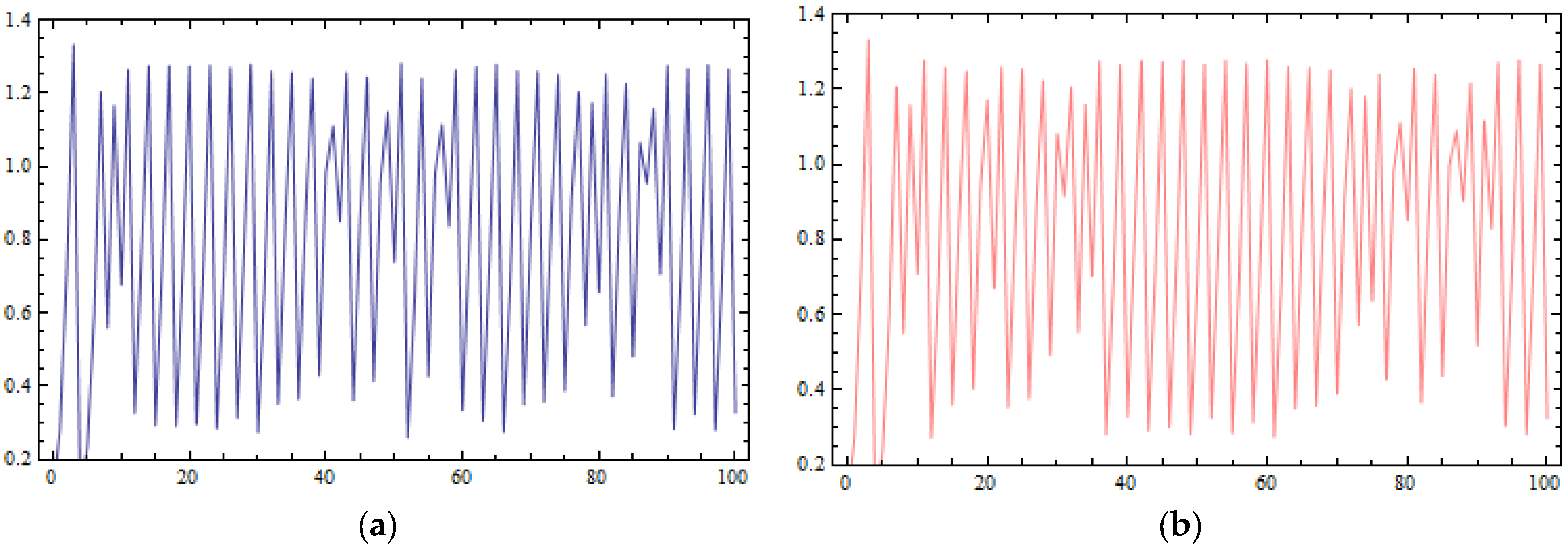
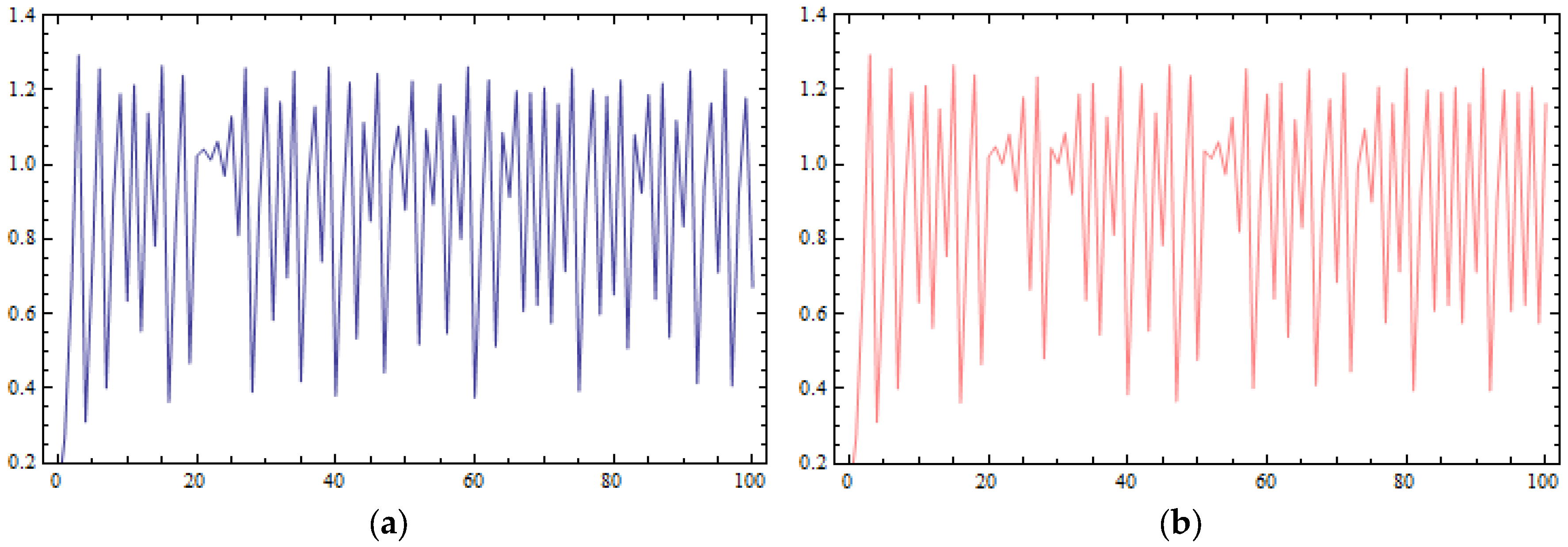
Another indication of the chaotic behavior caused by large values of parameter k is the sensitivity of the D.D.S. of Equation (38) in its initial conditions. In Figure 7a,b, the time series of two different initial conditions, (0.1, 0.1) (Figure 7a) and (0.101, 0.1) (Figure 7b), are plotted. At the first iterations of the time series, choosing the value of it seems that they are identical, but later, differences between them appear.
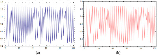
Figure 7.
Sensitive dependence on initial conditions for q1 coordinate plotted against the time of the system of Equation (16) for : (a) the orbit of (0.1, 0.1); (b) the orbit of (0.101, 0.1).
5. Chaos Control of the Modified Game
5.1. Application of the Delayed Feedback Control Method to the Modified Game
The delayed feedback method is applied to control the chaotic behavior that arises when the speed of adjustment (parameter k) takes values outside the stability space. In this modified game with the cubic cost function for the second player, the same control signal of Equation (14) is selected and the D.D.S. takes the following form:
The authors search to find the values (interval) of the control parameter m, which allow the N.E. of this new D.D.S. of Equation (47) to remain locally asymptotically stable even if parameter k takes values outside the stability space.
5.2. The Nash Equilibrium and Local Stability of the Modified Game Under the Control Parameter
The calculation of the N.E. is independent from parameters k or m and it has the same coordinates as those of the N.E., , of Section 4. The following proposition gives the local stability conditions for the N.E. of the D.D.S. of Equation (47).
Proposition 3.
The N.E. position of the D.D.S. of Equation (16) is locally asymptotically stable if:
and
Proof.
The Jacobian matrix of D.D.S. of Equation (47) is calculated as follows:
Using the three inequalities of Equation (31) for the Jacobian matrix of Equation (50), they become as follows:
that is the first local stability condition of the N.E.
an inequality that is always satisfied.
which is the second local stability condition. □
5.3. Numerical Simulations of the Modified Game Under the Control Parameter
Taking into account the local stabilities of Proposition 3 and setting the same values of the game’s parameters, , creates a two-dimensional space, which is presented in Figure 8.
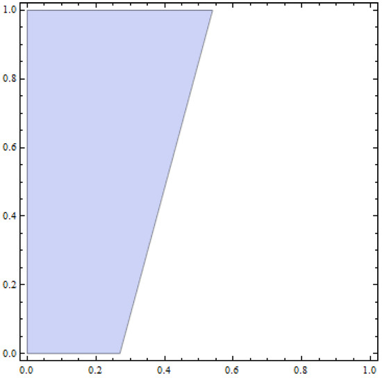
Figure 8.
Stability region of Equations (48) and (49) between parameters k, speed of adjustment (horizontal axis), and m, control parameter (vertical axis), for .
If is additionally set, then the local stabilities of Proposition 3 give the following common solutions as the local stability space for the control parameter m:
This result is verified by the bifurcation diagrams of (Figure 9a) and (Figure 9b) with respect to parameter m. When the speed of adjustment (parameter k) takes a value outside the stability space, e.g., and parameter m takes values larger than 0.85, then the N.E. is locally asymptotically stable. For values of the control parameter m smaller than 0.85, period-doubling bifurcations appear.
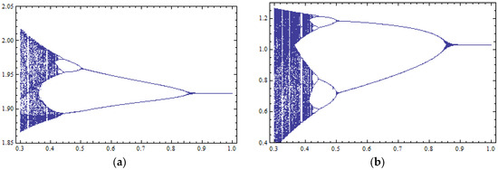
Figure 9.
Bifurcation diagrams with respect to the control parameter m (horizontal axis) with 400 iterations of the map of Equation (47) for : (a) against variable ; (b) against variable .
For small values of the control parameter m, e.g., , chaotic attractors (Figure 10a) are plotted and Lyapunov numbers (Figure 10b) larger than 1 are calculated. This chaotic ordit for the D.D.S. of Equation (47) makes the system sensitive in its initial conditions. In Figure 11a,b, the time series of coordinate for two different initial conditions, (0.1, 0.1) and (0.101, 0.1), are presented. It seems that only a small change in the first coordinate of the initial condition is capable of causing chaos and making the system unpredictable.
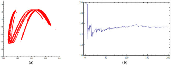
Figure 10.
Numerical simulations of the orbit of (0.1, 0.1) of the map of Equation (47) for : (a) phase portrait (chaotic attractor) with 8000 iterations; (b) Lyapunov numbers’ graph.
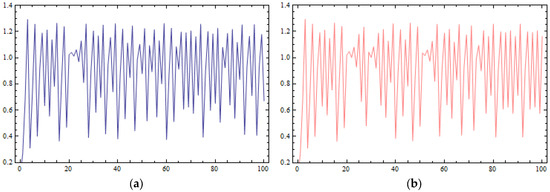
Figure 11.
Sensitive dependence on initial conditions for q1 coordinate plotted against the time of the system of Equation (47) for : (a) the orbit of (0.1, 0.1); (b) the orbit of (0.101, 0.1).
6. Conclusions
In this study, the authors present the delayed feedback method as an attempt to control the chaotic behavior of the Discrete Dynamical System (D.D.S.) that arises for large values of the speed of adjustment in a Cournot duopoly game with asymmetric cost functions, differentiated products, relative profit maximization and homogeneous expectations [27]. The asymmetric cost functions can capture the possible asymmetries/heterogeneities in firms’ technologies or firms’ input costs, making the model closer to economic reality [37]. The delayed feedback control method is applied on a Cournot duopoly game with quadratic cost function (Section 2 and Section 3), as well as with cubic cost function (Section 4 and Section 5). The cubic cost function is widely used in the Economic Dispatch Problem. The application of the delayed feedback method is achieved through the introduction of a control sign containing the control parameter m.
From the dynamic analysis of the Modified Game (Section 4 and Section 5), it is algebraically shown that the control parameter is capable of controlling the chaotic trajectories of the system that arise when the speed of adjustment takes values outside its local stability region, even if the two players use asymmetric cost functions. In addition to the analytical investigation of the model, the two local stability conditions of the Nash Equilibrium (N.E.) are verified through numerical simulations for specific values of the other parameters, such as plotting bifurcation diagrams and phase portraits (chaotic attractors), calculating Lyapunov numbers and making a sensitivity analysis of the system’s initial conditions.
From the stability region between the speed of adjustment and the control parameter, a useful result arises that the larger the value of the control parameter, the larger the local stability interval for the speed of adjustment. Finally, small values of the control parameter are not able to control the chaotic behavior of the system, and the destabilization of the N.E. appears through period-doubling bifurcations.
An interesting extension of this work is to consider a control signal with time lag . This will be addressed in future work.
Author Contributions
Conceptualization, K.P., G.S. and E.I.; methodology, K.P., G.S. and E.I.; software, K.P., G.S. and E.I.; validation, K.P., G.S. and E.I.; formal analysis, K.P., G.S. and E.I.; investigation, K.P., G.S. and E.I.; resources, K.P., G.S. and E.I.; data curation, K.P., G.S. and E.I.; writing—original draft preparation, K.P., G.S. and E.I.; writing—review and editing, K.P., G.S. and E.I.; visualization, K.P., G.S. and E.I.; All authors have read and agreed to the published version of the manuscript.
Funding
This research received no external funding.
Data Availability Statement
The original contributions presented in this study are included in the article. Further inquiries can be directed to the corresponding author.
Acknowledgments
We thank the anonymous reviewers, whose constructive criticism has significantly improved the presentation of this work.
Conflicts of Interest
The authors declare no conflicts of interest.
References
- Cournot, A.A. Researches into the Mathematical Principles of the Theory of Wealth; Irwin: Homewood, IL, USA, 1963. [Google Scholar]
- Agiza, H.N. On the analysis of stability, bifurcation, chaos and chaos control of Kopel map. Chaos Solitons Fractals 1999, 10, 1909–1916. [Google Scholar] [CrossRef]
- Agiza, H.N.; Hegazi, A.S.; Elsadany, A.A. Complex dynamics and synchronization of duopoly game with bounded rationality. Math. Comput. Simul. 2002, 58, 133–146. [Google Scholar] [CrossRef]
- Agliari, A.; Gardini, L.; Puu, T. Some global bifurcations related to the appearance of closed invariant curves. Math. Comput. Simul. 2005, 68, 201–219. [Google Scholar] [CrossRef]
- Agliari, A.; Gardini, L.; Puu, T. Global bifurcations in duopoly when the Cournot point is destabilized via a subcritical Neimark bifurcation. Int. Game Theory Rev. 2006, 8, 1–20. [Google Scholar] [CrossRef]
- Bishi, G.I.; Kopel, M. Equilibrium selection in a nonlinear duopoly game with adaptive expectations. J. Econ. Behav. Organ. 2001, 46, 73–100. [Google Scholar] [CrossRef]
- Kopel, M. Simple and complex adjustment dynamics in Cournot duopoly models. Chaos Solitons Fractals 1996, 7, 2031–2048. [Google Scholar] [CrossRef]
- Puu, T. The chaotic duopolists revisited. J. Econ. Behav. Organ. 1998, 33, 385–394. [Google Scholar] [CrossRef]
- Sarafopoulos, G. Complexity in a duopoly game with homogeneous players, convex, log linear demand and quadratic cost functions. Procedia Econ. Financ. 2015, 33, 358–366. [Google Scholar] [CrossRef]
- Sarafopoulos, G.; Papadopoulos, K. Chaos in oligopoly models. Int. J. Product. Manag. Assess. Technol. 2019, 7, 50–76. [Google Scholar] [CrossRef]
- Agiza, H.N.; Elsadany, A.A. Nonlinear dynamics in the Cournot duopoly game with heterogeneous players. Physica A 2003, 320, 512–524. [Google Scholar] [CrossRef]
- Agiza, H.N.; Elsadany, A.A. Chaotic dynamics in nonlinear duopoly game with heterogeneous players. Appl. Math. Comput. 2004, 149, 843–860. [Google Scholar] [CrossRef]
- Den Haan, W.J. The importance of the number of different agents in a heterogeneous asset-pricing model. J. Econ. Dyn. Control. 2001, 25, 721–746. [Google Scholar] [CrossRef]
- Fanti, L.; Gori, L. The dynamics of a differentiated duopoly with quantity competition. Econ. Model. 2012, 29, 421–427. [Google Scholar] [CrossRef]
- Hommes, C.H. Heterogeneous agents models in economics and finance. In Handbook of Computational Economics, Agent-Based Computational Economics; Tesfatsion, L., Judd, K.L., Eds.; Elsevier Science B.V.: Amsterdam, The Netherlands, 2006; Volume 2, pp. 1109–1186. [Google Scholar] [CrossRef]
- Sarafopoulos, G. On the dynamics of a duopoly game with differentiated goods. Procedia Econ. Financ. 2015, 19, 146–153. [Google Scholar] [CrossRef]
- Sarafopoulos, G.; Papadopoulos, K. On a Cournot Duopoly Game with Differentiated Goods, Heterogeneous Expectations and a Cost Function Including Emission Costs. Sci. Bull.–Econ. Sci. 2017, 1, 11–22. Available online: http://economic.upit.ro/RePEc/pdf/2017_1_2.pdf (accessed on 17 July 2025).
- Tramontana, F. Heterogeneous duopoly with isoelastic demand function. Econ. Model. 2010, 27, 350–357. [Google Scholar] [CrossRef]
- Baumol, W.J.; Quandt, R.E. Rules of thumb and optimally imperfect decisions. Am. Econ. Rev. 1964, 54, 23–46. Available online: https://www.jstor.org/stable/1810896 (accessed on 17 July 2025).
- Puu, T. The chaotic monopolist. Chaos Solitons Fractals 1995, 5, 35–44. [Google Scholar] [CrossRef]
- Naimzada, A.K.; Ricchiuti, G. Complex dynamics in a monopoly with a rule of thumb. Appl. Math. Comput. 2008, 203, 921–925. [Google Scholar] [CrossRef]
- Askar, S.S. On complex dynamics of monopoly market. Econ. Model. 2013, 31, 586–589. [Google Scholar] [CrossRef]
- Askar, S.S. Complex dynamics properties of Cournot duopoly games with convex and log-concave demand function. Oper. Res. Lett. 2014, 42, 85–90. [Google Scholar] [CrossRef]
- Bischi, G.I.; Gallegati, M.; Naimzada, A. Symmetry-breaking bifurcations and representative firm in dynamic duopoly games. Ann. Oper. Res. 1999, 89, 253–272. [Google Scholar] [CrossRef]
- Bischi, G.I.; Naimzada, A. Global Analysis of a Dynamic Duopoly Game with Bounded Rationality. Advances in Dynamic Games and Applications. In Advances in Dynamic Games and Applications; Filar, J.A., Gaitsgory, V., Mizukami, K., Eds.; Annals of the International Society of Dynamic Games; Birkhäuser: Boston, MA, USA, 2000; Volume 5. [Google Scholar] [CrossRef]
- Naimzada, A.K.; Sbragia, L. Oligopoly games with nonlinear demand and cost functions: Two boundedly rational adjustment processes. Chaos Solitons Fractals 2006, 29, 707–722. [Google Scholar] [CrossRef]
- Elsadany, A.A. Dynamics of a Cournot duopoly game with bounded rationality based on relative profit maximization. Appl. Math. Comput. 2017, 294, 253–263. [Google Scholar] [CrossRef]
- Satoh, A.; Tanaka, Y. Relative Profit Maximization and Equivalence of Cournot and Bertrand Equilibria in Asymmetric Differentiated Duopoly. Econ. Bull. 2014, 34, 819–827. Available online: https://mpra.ub.uni-muenchen.de/55895/1/MPRA_paper_55895.pdf (accessed on 17 July 2025).
- Sarafopoulos, G.; Papadopoulos, K. Dynamics of a Cournot game with differentiated goods and asymmetric cost functions based on relative profit maximization. Eur. J. Interdiscip. Stud. 2019, 2, 41–56. [Google Scholar] [CrossRef]
- Du, J.; Huang, T.; Sheng, Z. Analysis of decision-making in economic chaos control. Nonlinear Anal. Real World Appl. 2009, 10, 2493–2501. [Google Scholar] [CrossRef]
- Holyst, J.; Urbanowicz, K. Chaos control in economical model by time-delayed feedback method. Physica A 2000, 287, 587–598. [Google Scholar] [CrossRef]
- Ding, J.; Mei, Q.; Yao, H. Dynamics and adaptive control of a duopoly advertising model based on heterogeneous expectations. Nonlinear Dyn. 2012, 67, 129–138. [Google Scholar] [CrossRef]
- Elabbasy, E.M.; Agiza, H.N.; Elsadany, A.A. Analysis of nonlinear triopoly game with heterogeneous players. Comput. Math. Appl. 2009, 57, 488–499. [Google Scholar] [CrossRef]
- Pu, X.; Ma, J. Complex dynamics and chaos control in nonlinear four-oligopolist game with different expectations. Int. J. Bifurc. Chaos 2013, 23, 1350053. [Google Scholar] [CrossRef]
- Wei, Z.; Tan, W.; Elsadany, A.A.; Moroz, I. Complexity and chaos control in a Cournot duopoly model based on bounded rationality and relative profit maximizations. Nonlinear Dyn. 2023, 111, 17561–17589. [Google Scholar] [CrossRef]
- Agiza, H.N.; Elsadany, A.A.; El-Dessoky, M.M. On a new Cournot duopoly game. J. Chaos 2013, 1, 487803. [Google Scholar] [CrossRef]
- Pyragas, K. Continuous control of chaos by self-controlling feedback. Phys. Lett. 1992, 170, 421–428. [Google Scholar] [CrossRef]
- Kotsios, S. Feedback Control Techniques for a Discrete Dynamic Macroeconomic Model with Extra Taxation: An Algebraic Algorithm Approach. Mathematics 2023, 11, 4213. [Google Scholar] [CrossRef]
- Onozaki, T. Nonlinearity, Bounded Rationality, and Heterogeneity; Springer: Tokyo, Japan, 2018. [Google Scholar] [CrossRef]
- Singh, N.; Vives, X. Price and quantity competition in a differentiated duopoly. RAND J. Econ. 1984, 15, 546–554. [Google Scholar] [CrossRef]
- Li, T.; Ma, J. Complexity analysis of dual-channel game model with different managers’ business objectives. Commun. Nonlinear Sci. Numer. Simul. 2015, 20, 199–208. [Google Scholar] [CrossRef]
- Kulenovic, M.; Merino, O. Discrete Dynamical Systems and Difference Equations with Mathematica; Chapman & Hall/CRC: Boca Raton, FL, USA, 2002. [Google Scholar]
- Theerthamalai, A.; Maheswarapu, S. An effective non-iterative “λ-logic based” algorithm for economic dispatch of generators with cubic fuel cost function. Electr. Power Energy Syst. 2010, 32, 539–542. [Google Scholar] [CrossRef]
- Durai, S.; Subramanian, S.; Ganesan, S. Improved parameters for economic dispatch problems by teaching learning optimization. Int. J. Electr. Power Energy Syst. 2015, 67, 11–24. [Google Scholar] [CrossRef]
- Mahdi, F.P.; Vasant, P.; Abdullah-Al-Wadud, M.; Kallimani, V.; Watada, J. Quantum-behaved bat algorithm for many-objective combined economic emission dispatch problem using cubic criterion function. Neural Comput. Appl. 2019, 31, 5857–5869. [Google Scholar] [CrossRef]
- Hassan, M.H.; Yousri, D.; Kamel, S.; Rahmann, C. Amodified Marine predators algorithm for solving single-and multi-objective combined economic emission dispatch problems. Comput. Ind. Eng. 2022, 164, 107906. [Google Scholar] [CrossRef]


Disclaimer/Publisher’s Note: The statements, opinions and data contained in all publications are solely those of the individual author(s) and contributor(s) and not of MDPI and/or the editor(s). MDPI and/or the editor(s) disclaim responsibility for any injury to people or property resulting from any ideas, methods, instructions or products referred to in the content. |
© 2025 by the authors. Licensee MDPI, Basel, Switzerland. This article is an open access article distributed under the terms and conditions of the Creative Commons Attribution (CC BY) license (https://creativecommons.org/licenses/by/4.0/).