Numerical Analysis for a Class of Variational Integrators

Abstract

In this paper, we study a geometric framework for second-order differential systems arising in classical and relativistic mechanics. For this class of systems, we derive necessary and sufficient conditions for their Lagrangian description. The main objectives of this work are to construct efficient structure-preserving variational integrators in a variational framework. To achieve this, we develop new variational integrators through Lagrangian splitting and prove their equivalence to composition methods. We display the superiority of the newly derived numerical methods for the Kepler problem and provide rigorous error estimates by analysing the Laplace–Runge–Lenz vector. The framework provides tools applicable to geometric numerical integration of both ordinary and partial differential equations.

1. Introduction

Some important physical problems, ranging from celestial mechanics to magnetized plasmas, naturally exhibit rich conservative invariants. These problems are often described using geometric structures, which have attracted increasing interest in recent studies [1,2,3]. Examples of such structures include Hamiltonian, volume-preserving, Poisson, contact, and integral-preserving systems. Among these, variational structures play a central role in modelling systems in various applications. The inverse problem of mechanics has a long history. It can be traced back to Helmholtz’s foundational work [4] in 1887. This work was pursued further in 1941 by Douglas, who solved the two-dimensional case [5]. Vainberg later extended the framework to operator-theoretic settings applicable to partial differential equations [6]. We refer the reader to [7] for a more comprehensive review.

In the variational framework, variational integrators are constructed by discretizing the Lagrangian. Numerical methods are then derived via the discrete Euler–Lagrange equations. Through discrete Legendre transformations, variational integrators connect to symplectic methods in the Hamiltonian framework. Further details can be found in [8] and related references. For discrete Lagrangian systems, conservative numerical methods can be developed by studying variational symmetries and constructing a discrete Noether’s theorem [9,10]. Variational integrators have been successfully applied to simulate various physical problems, including soliton wave equations [11,12], charged particle dynamics in electromagnetic fields [13,14,15,16], and kinetic models in plasma physics [17,18]. Additionally, the construction and analysis of variational integrators have recently been applied to develop accelerated optimization methods [19,20].

In the theory of backward error analysis (or modified equations theory), a numerical method is interpreted as the exact solution of a nearby ’modified’ system. Structure-preserving numerical methods satisfy modified equations that retain the same structure as the original system, explaining their superior long-term behavior [21,22,23]. The concept has been extended to variational equations [24], adaptive time-step variational integrators [25], and Hamiltonian partial differential equations [26,27].

This paper focuses on second-order ordinary differential systems that model important physical problems. We establish necessary and sufficient conditions for variational formulations of this class of systems. The framework applies to classical/relativistic dynamics and charged particle motion under Lorentz forces. We introduce new variational integrators via Lagrangian splitting and prove their equivalence to composition methods through Legendre transformations. As a key example, we consider the Kepler problem—a super-integrable system modelling gravitational motion [28] with conserved energy, angular momentum, and the Laplace–Runge–Lenz (LRL) vector. The LRL vector [29] governs orbital geometry as a hidden conserved quantity. Due to its rich conservative properties, geometric integrators play a vital role in long-term Kepler simulations [30]. Using Levi–Civita transforms, exact schemes preserving all conserved quantities were constructed in [31,32]. We investigate our variational integrators’ performance on the Kepler problem. Using Noether’s theorem [33], we demonstrate variational symmetries for energy, momentum, and LRL vector. By developing modified equations and Lagrangians, we interpret numerical solutions as exact solutions of perturbed systems. Analysis shows the modified Kepler equation remains integrable but loses super-integrability, resulting in quasi-periodic orbits. We explicitly derive modified Lagrangians for symplectic Euler, Störmer–Verlet, and our new integrators. Perturbation theory reveals super-convergence in preserving the LRL vector, verifying the numerical performance.

The paper is organized as follows. Section 2 establishes the necessary and sufficient conditions for describing second-order systems within a variational framework. Section 3 constructs variational discretizations by splitting the Lagrangian. The resulting numerical discretization is shown to be equivalent to the composition method. Using classical and relativistic Kepler systems as examples, we illustrate the numerical methods and present variational symmetries for energy, momentum, and the LRL vector. Section 4 develops the theory of modified equations and modified Lagrangians. The recursive expressions for the Nyström methods are provided. For the Kepler problem, we also analyze the errors of the newly proposed variational integrators in conserving quantities. In Section 5, we apply the newly derived variational integrators to solve the Kepler problem. The numerical results demonstrate the superior performance of these methods. We further analyze the numerical performance using the modified Lagrangian theory. Additionally, we apply the variational integrators to solve the relativistic Kepler system. Finally, Section 6 concludes the paper.

2. Variational Principle in Lagrangian Formalism

We begin this section by introducing the inverse variational methods presented in [4,6,7,34]. Let $\mathcal{H}$ be a real Hilbert space with inner product $\langle ·,·\rangle$. Let $N:\mathcal{H}\to \mathcal{H}$ be an operator. The operator N is called symmetric if $N=N^{*}$, where $N^{*}$ is the adjoint operator defined by $\langle N^{*}u,v\rangle :=\langle u,Nv\rangle$ for $u,v\in \mathcal{H}$. The Fréchet derivative of N at $x\in \mathcal{H}$, denoted $N_x$, is the linear operator satisfying

$$N_x\delta u={\left.{\displaystyle \frac{d}{d\epsilon }}\right|}_{\epsilon =0}N(x+\epsilon \delta u),x,\delta u\in \mathcal{H}.$$

Theorem 1

(Vainberg’s theorem [6]). Let N be a operator defined on $\mathcal{H}$. If and only if the Fréchet derivative of N is symmetric, i.e. $N_x=N_x^{*}$, then there exists a functional S on $\mathcal{H}$, constructed as

$$S\left(x\right)={\int }_0^1\int x·N\left(\lambda x\right)d\lambda dt,$$

such that $N={\displaystyle \frac{\delta S}{\delta x}}$, where the variational derivative ${\displaystyle \frac{\delta S}{\delta x}}$ is defined by ${\left.{\displaystyle \frac{d}{dϵ}}\right|}_{ϵ=0}S(x+ϵ\delta u)=〈{\displaystyle \frac{\delta S}{\delta x}},\delta u〉$, $\forall \delta u\in \mathcal{H}$.

Remark 1.

In Theorem 1, setting $N=A(t,x,\dot{x})\ddot{x}-B(t,x,\dot{x})$ yields the Helmholtz conditions [4]. This establishes that a second-order differential system of the form $A(t,x,\dot{x})\ddot{x}=B(t,x,\dot{x})$ admits a variational description if and only if it is self-adjoint. Further details are provided in [7].

In this paper, we consider the systems governed by

$${\displaystyle \frac{d}{dt}}\left(M(x,\dot{x})\dot{x}\right)=f(t,x,\dot{x}),x\in {\mathbb{R}}^n$$

(1)

where $M(x,\dot{x})$ is an $n\times n$ symmetric matrix.

Theorem 2.

System (1) admits a variational formulation if and only if

$$\begin{array}{cc}\hfill & \sum _{k=1}^n{\displaystyle \frac{\partial M_{ik}}{\partial {\dot{x}}_j}}{\dot{x}}_k=\sum _{k=1}^n{\displaystyle \frac{\partial M_{jk}}{\partial {\dot{x}}_i}}{\dot{x}}_k,\hfill \end{array}$$

(2)

$$\begin{array}{cc}\hfill & \sum _{k=1}^n\left({\displaystyle \frac{\partial M_{ik}}{\partial x_j}}+{\displaystyle \frac{\partial M_{jk}}{\partial x_i}}\right){\dot{x}}_k={\displaystyle \frac{\partial f_i}{\partial {\dot{x}}_j}}+{\displaystyle \frac{\partial f_j}{\partial {\dot{x}}_i}},\hfill \end{array}$$

(3)

$$\begin{array}{cc}\hfill & \sum _{k=1}^n{\displaystyle \frac{d}{dt}}\left({\displaystyle \frac{\partial M_{ik}}{\partial x_j}}{\dot{x}}_k\right)={\displaystyle \frac{\partial f_i}{\partial x_j}}-{\displaystyle \frac{\partial f_j}{\partial x_i}}+{\displaystyle \frac{d}{dt}}{\displaystyle \frac{\partial f_j}{\partial {\dot{x}}_i}}\hfill \end{array}$$

(4)

hold for all $i,j=1,\dots ,n$.

Proof. 

Define $N\left(x\right)={\displaystyle \frac{d}{dt}}\left(M\dot{x}\right)-f$. The variational calculus gives

$$N_x\delta u={\displaystyle \frac{d}{dt}}\left[M\delta \dot{u}+\sum _{k=1}^n\left({\displaystyle \frac{\partial M}{\partial {\dot{x}}_k}}\delta {\dot{u}}_k+{\displaystyle \frac{\partial M}{\partial x_k}}\delta u_k\right)\dot{x}\right]-{\displaystyle \frac{\partial f}{\partial x}}\delta u-{\displaystyle \frac{\partial f}{\partial \dot{x}}}\delta \dot{u}.$$

(5)

The adjoint of $N_x$ is defined as

$$\langle N_x^{*}\delta u,\delta v\rangle =\langle \delta u,N_x\delta v\rangle =〈{\displaystyle \frac{d}{dt}}\left[M\delta \dot{v}+\sum _{k=1}^n\left({\displaystyle \frac{\partial M}{\partial {\dot{x}}_k}}\delta {\dot{v}}_k+{\displaystyle \frac{\partial M}{\partial x_k}}\delta v_k\right)\dot{x}\right]-{\displaystyle \frac{\partial f}{\partial x}}\delta v-{\displaystyle \frac{\partial f}{\partial \dot{x}}}\delta \dot{v},\delta u〉.$$

Using integration by parts, we obtain

$$\begin{array}{cc}\hfill \langle N_x^{*}\delta u,\delta v\rangle & =-〈M\delta \dot{v}+\sum _{k=1}^n\left({\displaystyle \frac{\partial M}{\partial {\dot{x}}_k}}\delta {\dot{v}}_k+{\displaystyle \frac{\partial M}{\partial x_k}}\delta v_k\right)\dot{x},\delta \dot{u}〉-〈{\displaystyle \frac{\partial f}{\partial x}}\delta v+{\displaystyle \frac{\partial f}{\partial \dot{x}}}\delta \dot{v},\delta u〉\hfill \\ \hfill & =-〈M\delta \dot{u}+\left(\sum _{k=1}^n{\displaystyle \frac{\partial M}{\partial {\dot{x}}_k}}\delta {\dot{u}}_k\right)\dot{x}+{\left({\displaystyle \frac{\partial f}{\partial \dot{x}}}\right)}^{\top },\delta \dot{v}〉-〈\left(\sum _{k=1}^n{\displaystyle \frac{\partial M}{\partial x_k}}\delta u_k\right)\dot{x}+{\left({\displaystyle \frac{\partial f}{\partial x}}\right)}^{\top },\delta v〉\hfill \\ \hfill & =-〈{\displaystyle \frac{\partial }{\partial \dot{x}}}\left({\dot{x}}^{\top }{M}^{\top }\delta \dot{u}\right)+{\left({\displaystyle \frac{\partial f}{\partial \dot{x}}}\right)}^{\top },\delta \dot{v}〉-〈{\displaystyle \frac{\partial }{\partial x}}\left({\dot{x}}^{\top }{M}^{\top }\delta \dot{u}\right)+{\left({\displaystyle \frac{\partial f}{\partial x}}\right)}^{\top },\delta v〉\hfill \\ \hfill & =〈{\displaystyle \frac{d}{dt}}\left[{\displaystyle \frac{\partial }{\partial \dot{x}}}\left(\dot{x^{\top }}{M}^{\top }\delta \dot{u}\right)\right]-{\displaystyle \frac{\partial }{\partial x}}\left[{\dot{x}}^{\top }M\delta \dot{u}\right]-{\left({\displaystyle \frac{\partial f}{\partial x}}\right)}^{\top }\delta u+{\displaystyle \frac{d}{dt}}\left[{\left({\displaystyle \frac{\partial f}{\partial \dot{x}}}\right)}^{\top }\delta u\right],\delta v〉.\hfill \end{array}$$

This derivation relies on the following identities:

$$\begin{array}{cc}\hfill & \langle u,\dot{v}\rangle =-\langle \dot{u},v\rangle ,〈\left(\sum _{k=1}^n{\displaystyle \frac{\partial M}{\partial {\dot{x}}_k}}{\dot{v}}_k\right)\dot{x},\dot{u}〉=-〈\left(\sum _{k=1}^n{\displaystyle \frac{\partial M}{\partial {\dot{x}}_k}}{\dot{u}}_k\right)\dot{x},\dot{v}〉,\hfill \\ \hfill & M\delta \dot{u}+\left(\sum _{k=1}^n{\displaystyle \frac{\partial M}{\partial {\dot{x}}_k}}\delta {\dot{u}}_k\right)\dot{x}={\displaystyle \frac{\partial }{\partial \dot{x}}}\left({\dot{x}}^{\top }{M}^{\top }\delta \dot{u}\right),\left(\sum _{k=1}^n{\displaystyle \frac{\partial M}{\partial x_k}}\delta u_k\right)\dot{x}={\displaystyle \frac{\partial }{\partial x}}\left({\dot{x}}^{\top }{M}^{\top }\delta \dot{u}\right).\hfill \end{array}$$

Therefore,

$$N_x^{*}\delta u={\displaystyle \frac{d}{dt}}\left[{\displaystyle \frac{\partial }{\partial \dot{x}}}\left({\dot{x}}^{\top }{M}^{\top }\delta \dot{u}\right)\right]-{\displaystyle \frac{\partial }{\partial x}}\left[{\dot{x}}^{\top }M\delta \dot{u}\right]-{\left({\displaystyle \frac{\partial f}{\partial x}}\right)}^{\top }\delta u+{\displaystyle \frac{d}{dt}}\left[{\left({\displaystyle \frac{\partial f}{\partial \dot{x}}}\right)}^{\top }\delta u\right].$$

(6)

According to Theorem 1, the system is variational if and only if (5) and (6) are identical. Comparing (5) and (6) leads to

$$\begin{array}{cc}\hfill & \left[M_{ij}+\sum _{k=1}^n{\displaystyle \frac{\partial M_{ik}}{\partial {\dot{x}}_j}}{\dot{x}}_k-M_{ji}-\sum _{k=1}^n{\displaystyle \frac{\partial M_{jk}}{\partial {\dot{x}}_i}}{\dot{x}}_k\right]\delta {\ddot{u}}_j\hfill \\ \hfill +& \left[{\displaystyle \frac{d}{dt}}\left(M_{ij}+\sum _{k=1}^n{\displaystyle \frac{\partial M_{ik}}{\partial {\dot{x}}_j}}{\dot{x}}_k-M_{ji}-\sum _{k=1}^n{\displaystyle \frac{\partial M_{jk}}{\partial {\dot{x}}_i}}{\dot{x}}_k\right)+\sum _{k=1}^n\left({\displaystyle \frac{\partial M_{ik}}{\partial x_j}}+{\displaystyle \frac{\partial M_{jk}}{\partial x_i}}\right){\dot{x}}_k-{\displaystyle \frac{\partial f_i}{\partial {\dot{x}}_j}}-{\displaystyle \frac{\partial f_j}{\partial {\dot{x}}_i}}\right]\delta {\dot{u}}_j\hfill \\ \hfill +& \left[{\displaystyle \frac{d}{dt}}\left(\sum _{k=1}^n{\displaystyle \frac{\partial M_{ik}}{\partial x_j}}{\dot{x}}_k\right)-{\displaystyle \frac{\partial f_i}{\partial x_j}}+{\displaystyle \frac{\partial f_j}{\partial x_i}}-{\displaystyle \frac{d}{dt}}{\displaystyle \frac{\partial f_j}{\partial {\dot{x}}_i}}\right]\delta u_j=0.\hfill \end{array}$$

The above equality holds for arbitrary $u\in \mathcal{H}$. Thus, the coefficients in terms $\delta u$, $\delta \dot{u}$ and $\delta \ddot{u}$ vanish. Since M is symmetric, this implies exactly that

$$\begin{array}{cc}\hfill & \sum _{k=1}^n\left({\displaystyle \frac{\partial M_{ik}}{\partial {\dot{x}}_j}}{\dot{x}}_k-{\displaystyle \frac{\partial M_{jk}}{\partial {\dot{x}}_i}}{\dot{x}}_k\right)=0,\hfill \\ \hfill & \sum _{k=1}^n\left({\displaystyle \frac{\partial M_{ik}}{\partial x_j}}+{\displaystyle \frac{\partial M_{jk}}{\partial x_i}}\right){\dot{x}}_k-{\displaystyle \frac{\partial f_i}{\partial {\dot{x}}_j}}-{\displaystyle \frac{\partial f_j}{\partial {\dot{x}}_i}}=0,\hfill \\ \hfill & {\displaystyle \frac{d}{dt}}\left(\sum _{k=1}^n{\displaystyle \frac{\partial M_{ik}}{\partial x_j}}{\dot{x}}_k\right)-{\displaystyle \frac{\partial f_i}{\partial x_j}}+{\displaystyle \frac{\partial f_j}{\partial x_i}}-{\displaystyle \frac{d}{dt}}{\displaystyle \frac{\partial f_j}{\partial {\dot{x}}_i}}=0.\hfill \end{array}$$

This completes the proof of the theorem. □

Assuming $M=M\left(\dot{x}\right)$ and that f is linear in $\dot{x}$, we can rewrite the above theorem as follows:

Theorem 3.

For $M=M\left(\dot{x}\right)$ and $f=A(t,x)\dot{x}+\varphi (t,x)$, system (1) is variational if and only if

$$\begin{array}{cc}\hfill & \sum _{k=1}^n{\displaystyle \frac{\partial M_{ik}}{\partial {\dot{x}}_j}}{\dot{x}}_k=\sum _{k=1}^n{\displaystyle \frac{\partial M_{jk}}{\partial {\dot{x}}_i}}{\dot{x}}_k,\hfill \end{array}$$

$$\begin{array}{cc}\hfill & A(t,x)=-A^{\top }(t,x),\hfill \end{array}$$

(7)

$$\begin{array}{cc}\hfill & {\displaystyle \frac{\partial A_{jk}}{\partial x_i}}+{\displaystyle \frac{\partial A_{ki}}{\partial x_j}}+{\displaystyle \frac{\partial A_{ij}}{\partial x_k}}=0,\hfill \end{array}$$

(8)

$$\begin{array}{cc}\hfill & {\displaystyle \frac{\partial {\varphi }_i}{\partial x_j}}-{\displaystyle \frac{\partial {\varphi }_j}{\partial x_i}}={\displaystyle \frac{\partial A_{ij}}{\partial t}},\hfill \end{array}$$

(9)

where $i,j,k=1,\dots ,n$.

Proof. 

Since M depends only on $\dot{x}$, (3) simplifies to (7). The condition (4) reduces to

$$\sum _{k=1}^n\left({\displaystyle \frac{\partial A_{jk}}{\partial x_i}}+{\displaystyle \frac{\partial A_{ki}}{\partial x_j}}+{\displaystyle \frac{\partial A_{ij}}{\partial x_k}}\right){\dot{x}}_k={\displaystyle \frac{\partial A_{ji}}{\partial t}}+{\displaystyle \frac{\partial {\varphi }_i}{\partial x_j}}-{\displaystyle \frac{\partial {\varphi }_j}{\partial x_i}}.$$

In the above equality, the term on the right-hand side does not depend on $\dot{x}$, so the coefficients of $\dot{x}$ vanish. □

Remark 2.

Define a differential two-form by $\omega ={\displaystyle \frac{1}{2}}dx\wedge Adx$. If (7) and (8) hold, then $d\omega =0$. By Poincaré’s lemma, there exists a one-form $\beta =gdx$ such that $\omega =d\beta$. This implies $A={\nabla }_x{g}^{\top }-{\nabla }_{x}g$. Condition (9) means that ϕ can be generated from a potential ϕ by $\varphi =-{\nabla }_x\varphi -{\displaystyle \frac{\partial g}{\partial t}}$.

In more classical applications, M is typically a constant matrix. In this case, for the system to be variational, we only need the conditions for the vector field f.

Theorem 4.

For constant symmetric M, system (1) is variational if

$$\begin{array}{cc}\hfill & {\displaystyle \frac{\partial f_i}{\partial {\dot{x}}_j}}+{\displaystyle \frac{\partial f_j}{\partial {\dot{x}}_i}}=0,\hfill \end{array}$$

(10)

$$\begin{array}{cc}\hfill & {\displaystyle \frac{\partial f_i}{\partial x_j}}-{\displaystyle \frac{\partial f_j}{\partial x_i}}+{\displaystyle \frac{d}{dt}}{\displaystyle \frac{\partial f_i}{\partial {\dot{x}}_j}}=0\hfill \end{array}$$

(11)

holds for $i,j,k=1,\dots ,n$.

Many important physical problems, including some relativistic models, can take the form of Theorem 3. Consider the relativistic dynamics (such as a charged particle in a Coulomb potential)

$${\displaystyle \frac{d}{dt}}\left(\gamma \left(\dot{x}\right)\dot{x}\right)=-\nabla \varphi \left(x\right)$$

(12)

where $\gamma \left(\dot{x}\right):=(1-|\dot{x}{{|}^2/c^2)}^{-1/2}$ is the Lorentz factor, and c is the speed of light. In the non-relativistic limit ($|\dot{x}|\ll c$), this reduces to Newtonian mechanics $\ddot{x}=-\nabla \varphi \left(x\right)$. It is evident that the velocity-dependent terms satisfy the symmetry conditions (2) and (9). This system admits the variational formulation with Lagrangian $L(x,\dot{x})=-c^2{\gamma }^{-1}\left(\dot{x}\right)+\varphi \left(x\right)$.

It is well known that from a Lagrangian framework it is more convenient to investigate the connections between conservation laws and symmetry properties of dynamical systems based on Noether’s theorem. The foundational framework requires introducing generalized vector fields and their action on variational principles [34].

A generalized vector field is given by

$$\mathbf{v}=\sum _{i=1}^n{v}_i\left[x\right]{\displaystyle \frac{\partial }{\partial x_i}}$$

where $v_i\left[x\right]$ contains x, and all the derivatives of x and $v=(v_1,...,v_n)$ denote its characteristic. The infinite prolongation of $\mathbf{v}$ is defined as

$$pr\mathbf{v}=\mathbf{v}+\sum _{i=1}^n\sum _{j=1}^{\infty }{\displaystyle \frac{d^j{v}_i}{d{t}^j}}{\displaystyle \frac{\partial }{\partial x_i^{\left(j\right)}}}$$

where $x_i^{\left(j\right)}:={\displaystyle \frac{d^j{x}_i}{d^{j}t}}$ denotes j-th order time derivatives.

Definition 1

([34], Chapter 5). A generalized vector field $\mathbf{v}$ is called a variational symmetry for the functional $S\left[x\right]=\int L\left[x\right]dt$ if there exists a function $K\left[x\right]$ such that

$$pr\mathbf{v}\left(L\right)={\displaystyle \frac{d}{dt}}K\left[x\right].$$

Given a differential system $N\left[x\right]=0$, if there exists $Q\left[x\right]$ satisfying

$${\displaystyle \frac{dP}{dt}}=N\left[x\right]·Q,$$

then Q is called the characteristic of the nontrivial conservation law ${\displaystyle \frac{dP}{dt}}=0$.

Theorem 5

(Noether’s theorem, see [34], Chapter 5). A generalized vector field $\mathbf{v}$ is a variational symmetry if and only if its characteristic Q is also the characteristic of a conservation law ${\displaystyle \frac{dP}{dt}}=0$ along the solution of Euler–Lagrange equations.

When the system is perturbed, the following proposition holds:

Proposition 1.

Given a Lagrangian L, let $\mathbf{v}$ and P denote its variational symmetry and the corresponding conserved quantity, respectively. Under the perturbed Lagrangian $\tilde{L}=L+\epsilon \overline{L}$, P along solutions of $EL\left(\tilde{L}\right)=0$ satisfies

$${\displaystyle \frac{dP}{dt}}=-\epsilon EL\left(\overline{L}\right)·v,$$

where $EL={\displaystyle \frac{\partial }{\partial x}}-{\displaystyle \frac{d}{dt}}{\displaystyle \frac{\partial }{\partial \dot{x}}}$ is the the Euler operator.

Proof. 

By Theorem 5, it gives ${\displaystyle \frac{dP}{dt}}=EL\left(L\right)·v$. For the solution of the perturbed system $EL\left(\tilde{L}\right)=0$, we have

$$EL\left(L\right)·v+\epsilon EL\left(\overline{L}\right)·v=0.$$

Substitution yields ${\displaystyle \frac{dP}{dt}}=-\epsilon EL\left(\overline{L}\right)·v$. □

3. Discrete Lagrangian Mechanics

Variational integrators preserve geometric structures by discretizing Hamilton’s principle. For foundational theory, see [8]. Consider a uniform time grid $t_n=t_0+nh$ with coordinates $x_n\in {\mathbf{R}}^{\mathrm{N}}$. The discrete Hamilton’s principle is to find the trajectories ${\left\{x_n\right\}}_{n=0}^{\mathrm{N}}$ extremizing the discrete action functional

$$\mathbb{S}\left({\left\{x_n\right\}}_{n=0}^{\mathrm{N}}\right)=h\sum _{n=0}^{\mathrm{N}-1}\mathbb{L}\left(x_n,x_{n+1},h\right).$$

(13)

Here, $\mathbb{L}$ is the discretization of L, given by $\mathbb{L}(x_n,x_{n+1},h)\approx {\displaystyle \frac{1}{h}}{\int }_{t_n}^{t_{n+1}}L(x,\dot{x})dt$. Its adjoint, denoted by ${\mathbb{L}}^{*}$, is defined as ${\mathbb{L}}^{*}(x_n,x_{n+1},h)=\mathbb{L}(x_{n+1},x_n,-h)$. The discrete solution $x_n$ satisfies the discrete Euler–Lagrange equations

$${\partial }_1\mathbb{L}(x_n,x_{n+1},h)+{\partial }_2\mathbb{L}(x_{n-1},x_n,h)=0.$$

Consider the system

$$\ddot{x}=-\nabla \varphi \left(x\right),x\in {\mathbf{R}}^{\mathrm{N}},$$

(14)

with Lagrangian $L(x,\dot{x})={\displaystyle \frac{1}{2}}{\dot{x}}^2-\varphi \left(x\right)$. We discretize the Lagrangian to obtain the variational integrators. By splitting the potential $\varphi \left(x\right)$ as $\varphi \left(x\right)={\displaystyle \sum _{i=1}^N}{\varphi }^{\left[i\right]}\left(x\right)$, we present the following discrete Lagrangian, a first-order variational integrator uses the discrete Lagrangian:

$${\mathbb{L}}^{1\mathrm{st}}(x_n,x_{n+1},h)={\displaystyle \frac{1}{2}}{\displaystyle \frac{|x_{n+1}-x_n{|}^2}{h^2}}-\sum _{i=1}^N{\varphi }^{\left[i\right]}\left({\widehat{x}}_n^i\right)$$

(15)

where ${\widehat{x}}_n^i:=x_n+{\displaystyle \sum _{j=1}^i}(x_{n+1}^j-x_n^j){\mathbf{e}}_j$, ${\mathbf{e}}_j$ is the N-dimensional vector with the j-th element being 1.

Theorem 6.

The discrete Lagrangian is of order 1. Moreover, the discrete Euler–Lagrange equations for (15) generate

$$\begin{array}{c}\hfill {\displaystyle \frac{x_{n+1}^i-2x_n^i+x_{n-1}^i}{h^2}}=-{\displaystyle \frac{\partial }{\partial x_i}}\left(\sum _{j=1}^{i-1}{\varphi }^{\left[j\right]}\left({\widehat{x}}_n^j\right)+\sum _{j=i}^{\mathrm{N}}{\varphi }^{\left[j\right]}\left({\widehat{x}}_{n-1}^j\right)\right),i=1,\dots ,\mathrm{N}.\end{array}$$

This coincides with the composition method

$${\Phi }_h={\Phi }_{H_N}^h\circ \cdots \circ {\Phi }_{H_1}^h,$$

where $H_i={\displaystyle \frac{1}{2}}{p}_i^2+{\varphi }^{\left[i\right]}\left(x\right)$ represents the subsystem, and ${\Phi }_{H_i}^h$ is the corresponding numerical discretization, given by

$$x_{n+1}=x_n+h{\displaystyle \frac{\partial H^{\left[i\right]}}{\partial p}}(x_{n+1},p_n),p_{n+1}=p_n-h{\displaystyle \frac{\partial H^{\left[i\right]}}{\partial x}}(x_{n+1},p_n).$$

Proof. 

Using the Taylor expansion at an arbitrary $t\in [t_n,t_{n+1}]$, we have

$${\displaystyle \frac{x\left(t_{n+1}\right)-x\left(t_n\right)}{h}}=\dot{x}\left(t\right)+\mathcal{O}\left(h\right),{\varphi }^{\left[i\right]}\left({\widehat{x}}^i\left(t_n\right)\right)={\varphi }^{\left[i\right]}\left(x\left(t\right)\right)+\mathcal{O}\left(h\right).$$

Substituting these into (15), it is easy to see that the discrete Lagrangian has first-order accuracy.

Introduce the discrete Legendre transformation

$$p_n=-h{\displaystyle \frac{\partial {\mathbb{L}}^{1\mathrm{st}}(x_n,x_{n+1})}{\partial x_n}}={\displaystyle \frac{x_{n+1}-x_n}{h}}+h\sum _{i=2}^{\mathrm{N}}{\displaystyle \frac{\partial }{\partial x_i}}\sum _{j=1}^{i-1}{\varphi }^{\left[j\right]}\left({\widehat{x}}_n^j\right){\mathbf{e}}_i.$$

(16)

The discrete Euler–Lagrange equation gives

$$p_{n+1}=h{\displaystyle \frac{\partial {\mathbb{L}}^{1\mathrm{st}}(x_n,x_{n+1})}{\partial x_{n+1}}}={\displaystyle \frac{x_{n+1}-x_n}{h}}+h\sum _{i=1}^{\mathrm{N}}{\displaystyle \frac{\partial }{\partial x_i}}\sum _{j=i}^{\mathrm{N}}{\varphi }^{\left[j\right]}\left({\widehat{x}}_n^j\right){\mathbf{e}}_i.$$

(17)

From (16) and (17), we can derive

$$\begin{array}{cc}\hfill & x_{n+1}=x_n+h{p}_n-h^2\sum _{i=2}^{\mathrm{N}}{\displaystyle \frac{\partial }{\partial x_i}}\sum _{j=1}^{i-1}{\varphi }^{\left[j\right]}\left({\widehat{x}}_n^j\right){\mathbf{e}}_i,\hfill \end{array}$$

(18)

$$\begin{array}{cc}\hfill & p_{n+1}=p_n-h\sum _{i=1}^{\mathrm{N}}\nabla {\varphi }^{\left[i\right]}\left({\widehat{x}}_n^i\right).\hfill \end{array}$$

(19)

This is exactly the composition method ${\Phi }_h$. □

The discrete Lagrangian of higher-order variational integrators can be constructed by combining $\mathbb{L}$ and its adjoint ${\mathbb{L}}^{*}$

$$\begin{array}{cc}\hfill {\mathbb{L}}^{2\mathrm{nd}}(x_n,x_{n+1},h)& ={\displaystyle \frac{1}{2}}{\mathbb{L}}^{1\mathrm{st}}(x_n,x_{n+1/2},h/2)+{\displaystyle \frac{1}{2}}{\mathbb{L}}^{*}(x_{n+1/2},x_{n+1},h/2),\hfill \end{array}$$

(20)

$$\begin{array}{cc}\hfill {\mathbb{L}}^{2\mathrm{nd}}(x_n,x_{n+1},h)& ={\displaystyle \frac{1}{2}}{\mathbb{L}}^{*}(x_n,x_{n+1/2},h/2)+{\displaystyle \frac{1}{2}}{\mathbb{L}}^{1\mathrm{st}}(x_{n+1/2},x_{n+1},h/2).\hfill \end{array}$$

(21)

By the discrete Euler–Lagrange equation, these provide the higher-order variational integrators.

Theorem 7.

The variational integrators from (20) and (21) are equivalent to ${\Phi }_h^{2\mathrm{nd}}={\Phi }_{h/2}^{*}\circ {\Phi }_{h/2}$ and ${\Phi }_h^{2\mathrm{nd}}={\Phi }_{h/2}\circ {\Phi }_{h/2}^{*}$, respectively.

Proof. 

The corresponding discrete Euler–Lagrange equation for (20) gives

$$\begin{array}{cc}\hfill & {\displaystyle \frac{\partial {\mathbb{L}}^{1\mathrm{st}}(x_n,x_{n+1/2},h/2)}{\partial x_n}}+{\displaystyle \frac{\partial {\mathbb{L}}^{*}(x_{n-1/2},x_n,h/2)}{\partial x_n}}=0,\hfill \end{array}$$

(22)

$$\begin{array}{cc}\hfill & {\displaystyle \frac{\partial {\mathbb{L}}^{1\mathrm{st}}(x_n,x_{n+1/2},h/2)}{\partial x_{n+1/2}}}+{\displaystyle \frac{\partial {\mathbb{L}}^{*}(x_{n+1/2},x_{n+1},h/2)}{\partial x_{n+1/2}}}=0.\hfill \end{array}$$

(23)

Introduce the discrete Legendre transformation,

$$\begin{array}{cc}\hfill p_n& =-{\displaystyle \frac{h}{2}}{\displaystyle \frac{\partial {\mathbb{L}}^{1\mathrm{st}}(x_n,x_{n+1/2},h/2)}{\partial x_n}},\hfill \end{array}$$

(24)

$$\begin{array}{cc}\hfill p_{n+1/2}& ={\displaystyle \frac{h}{2}}{\displaystyle \frac{\partial {\mathbb{L}}^{1\mathrm{st}}(x_n,x_{n+1/2},h/2)}{\partial x_{n+1/2}}},\hfill \end{array}$$

(25)

$$\begin{array}{cc}\hfill p_{n+1}& ={\displaystyle \frac{h}{2}}{\displaystyle \frac{\partial {\mathbb{L}}^{*}(x_{n+1/2},x_{n+1},h/2)}{\partial x_{n+1}}}.\hfill \end{array}$$

(26)

From (23), we know

$$p_{n+1/2}={\displaystyle \frac{h}{2}}{\displaystyle \frac{\partial {\mathbb{L}}^{1\mathrm{st}}(x_n,x_{n+1/2},h/2)}{\partial x_{n+1/2}}}=-{\displaystyle \frac{h}{2}}{\displaystyle \frac{\partial {\mathbb{L}}^{*}(x_{n+1/2},x_{n+1},h/2)}{\partial x_{n+1/2}}}.$$

(27)

Combine (24)–(26) and (27), we can prove that ${\Phi }_h^{2\mathrm{nd}}={\Phi }_{h/2}^{*}\circ {\Phi }_{h/2}$. □

As follows, we take the Kepler problem as an example to illustrate the newly derived variational methods of first and second order.

• Kepler problem. The Kepler problem describes the motion of two bodies attracting each other. We focus on the 2-dimensional Kepler problem in the following text. If one body is placed at the origin, and x represents the position of the other body, then their dynamics are governed by the following system:

  $$\ddot{x}=-\nabla \varphi \left(x\right),x\in {\mathbf{R}}^2,$$

  (28)

  where $\varphi \left(x\right)=-{\displaystyle \frac{1}{\left|x\right|}}$. It is obvious that the Kepler problem (28) satisfies Theorem 4, and its Lagrangian is given by

  $$L(x,\dot{x})={\displaystyle \frac{1}{2}}{\left|\dot{x}\right|}^2+{\displaystyle \frac{1}{\left|x\right|}}.$$

  (29)

The Kepler problem (28) has three conserved quantities: energy, angular momentum, and the Laplace–Runge–Lenz (LRL) vector. With the initial energy $H_0<0$, the solution orbit of the Kepler problem is elliptic, such as the motion of one astronomical body moving around another. In this case, the LRL vector determines the orientation and shape of the elliptical orbit. The magnitude $\left|\mathbf{A}\right|=\sqrt{A_1^2+A_2^2}$ equals the orbital eccentricity e, and the vector $\mathbf{A}$ points along the major axis of the orbit.

Proposition 2

([29], Chapter 6). For the 2D Kepler system (28), the following quantities are conserved:

• Energy  $H(x,\dot{x})={\displaystyle \frac{1}{2}}{\left|\dot{x}\right|}^2-{\displaystyle \frac{1}{\left|x\right|}}$,
• Angular Momentum  $m(x,\dot{x})=x_1{\dot{x}}_2-x_2{\dot{x}}_1$,
• LRL Vector  $\mathbf{A}(x,\dot{x})=(A_1,A_2)=\left(x_1|\dot{x}{|}^2-{\dot{x}}_1\left(x·\dot{x}\right)-{\displaystyle \frac{x_1}{\left|x\right|}},x_2{\left|\dot{x}\right|}^2-{\dot{x}}_2\left(x·\dot{x}\right)-{\displaystyle \frac{x_2}{\left|x\right|}}\right)$.

Based on Noether’s theorem, for the two-dimensional Kepler problem (28), we derive the variational symmetries corresponding to the three conservative quantities expressed in Proposition 2.

Proposition 3.

The variational symmetries associated with the energy, angular momentum, and the LRL vector are as follows:

• ${\mathbf{v}}_H=-{\dot{x}}_1{\displaystyle \frac{\partial }{\partial x_1}}-{\dot{x}}_2{\displaystyle \frac{\partial }{\partial x_2}}$,
• ${\mathbf{v}}_m=x_2{\displaystyle \frac{\partial }{\partial x_1}}-x_1{\displaystyle \frac{\partial }{\partial x_2}}$,
• ${\mathbf{v}}_{A_1}=x_2{\dot{x}}_2{\displaystyle \frac{\partial }{\partial x_1}}-\left(2x_1{\dot{x}}_2-{\dot{x}}_1{x}_2\right){\displaystyle \frac{\partial }{\partial x_2}}$, ${\mathbf{v}}_{A_2}=-\left(2x_2{\dot{x}}_1-x_1{\dot{x}}_2\right){\displaystyle \frac{\partial }{\partial x_1}}+x_1{\dot{x}}_1{\displaystyle \frac{\partial }{\partial x_2}}$.

Proof. 

Taking $N\left[\mathbf{x}\right]=-{\left({\ddot{x}}_1+{\displaystyle \frac{x_1}{{\left|\mathbf{x}\right|}^3}},{\ddot{x}}_2+{\displaystyle \frac{x_2}{{\left|\mathbf{x}\right|}^3}}\right)}^{\top }$ gives the following equality for energy conservation:

$${\displaystyle \frac{dH}{dt}}=-\dot{\mathbf{x}}·(-\ddot{\mathbf{x}}-\mathbf{x}/{\left|\mathbf{x}\right|}^3)=-\dot{\mathbf{x}}·\left(-N\left[\mathbf{x}\right]\right).$$

Suppose the generalized vector field ${\mathbf{v}}_H=-({\dot{x}}_1,{\dot{x}}_2)$. According to Theorem 5, ${\mathbf{v}}_H$ is exactly the variational symmetry of the energy. The other variational symmetries follow analogously from their conservation laws. □

Splitting $\varphi$ as $\varphi ={\varphi }^{\left[1\right]}+{\varphi }^{\left[2\right]}$, we construct the first-order and second-order discrete Lagrangians. The first-order Lagrangian (15) yields the variational integrator through the discrete Euler–Lagrange equations

$$\begin{array}{c}\hfill {\displaystyle \frac{x_{n+1}-2x_n+x_{n-1}}{h^2}}=-\left[\begin{array}{c}{\displaystyle \frac{\partial }{\partial x_1}}\left({\varphi }^{\left[1\right]}(x_n^1,x_{n-1}^2)+{\varphi }^{\left[2\right]}(x_n^1,x_n^2)\right)\hfill \\ {\displaystyle \frac{\partial }{\partial x_2}}\left({\varphi }^{\left[1\right]}(x_{n+1}^1,x_n^2)+{\varphi }^{\left[2\right]}(x_n^1,x_n^2)\right)\hfill \end{array}\right].\end{array}$$

(30)

The second-order Lagrangians (21) generate the numerical methods

$$\begin{array}{c}\hfill \begin{array}{cc}\hfill {\displaystyle \frac{x_{n+1/2}-2x_n+x_{n-1/2}}{{(h/2)}^2}}& =-\left[\begin{array}{c}{\displaystyle \frac{\partial }{\partial x_1}}\left({\varphi }^{\left[1\right]}(x_n^1,x_{n-1/2}^2)+2{\varphi }^{\left[2\right]}(x_n^1,x_n^2)+{\varphi }^{\left[1\right]}(x_n^1,x_{n+1/2}^2)\right)\\ {\displaystyle \frac{\partial }{\partial x_2}}\left(2{\varphi }^{\left[2\right]}(x_n^1,x_n^2)\right)\end{array}\right],\hfill \\ \hfill {\displaystyle \frac{x_{n+1}-2x_{n+1/2}+x_n}{{(h/2)}^2}}& =-\left[\begin{array}{c}0\\ {\displaystyle \frac{\partial }{\partial x_2}}\left({\varphi }^{\left[1\right]}(x_n^1,x_{n+1/2}^2)+{\varphi }^{\left[1\right]}(x_{n+1}^1,x_{n+1/2}^2)\right)\end{array}\right].\hfill \end{array}\end{array}$$

(31)

• Relativistic Kepler Problems. Considering the relativistic Kepler systems in (12) with the potential $\varphi \left(x\right)={\displaystyle \frac{1}{\left|x\right|}}$. With the proper time $\tau$ and relativistic momentum $u:=\gamma \left(\dot{x}\right)\dot{x}$, we reformulate system (12) as

  $${\displaystyle \frac{d}{d\tau }}\left[\begin{array}{c}t\\ x^{\top }\end{array}\right]=\left[\begin{array}{c}\gamma \\ u^{\top }\end{array}\right],{\displaystyle \frac{d}{d\tau }}\left[\begin{array}{c}\gamma \\ u^{\top }\end{array}\right]=\left[\begin{array}{cc}0& -\nabla {\varphi }^{\top }/c^2\\ -\nabla \varphi & 0\end{array}\right]\left[\begin{array}{c}\gamma \\ u^{\top }\end{array}\right],$$

  (32)

  where $\gamma \left(u\right)=\sqrt{{1+|u/c|}^2}$. Let $\mathbf{x}={(t,x^{\top })}^{\top }$ and $\dot{\mathbf{x}}={(\gamma ,u^{\top })}^{\top }$, where ’·’ denotes differentiation with respect to $\tau$. From Theorem 4, we learn that the system (32) admits a variational formulation with Lagrangian

  $$L(\mathbf{x},\dot{\mathbf{x}})={\displaystyle \frac{1}{2}}{\dot{\mathbf{x}}}^{\top }\mathbf{M}\dot{\mathbf{x}}+A\left(\mathbf{x}\right)·\dot{\mathbf{x}},$$

  (33)

  where $\mathbf{M}=\left[\begin{array}{cc}-c^2& 0\\ 0& {\mathbf{I}}_{\mathrm{N}}\end{array}\right]$ and $A\left(\mathbf{x}\right)=(-\varphi \left(x\right),{\mathbf{0}}_{1\times \mathrm{N}})$. The system (32) has two Hamiltonian formulations. Defining $p={\displaystyle \frac{\partial L}{\partial \dot{\mathbf{x}}}}=\mathbf{M}\dot{\mathbf{x}}+A\left(\mathbf{x}\right)$, the system (32) admits the standard Hamiltonian form

  $$\dot{y}=J^{-1}\nabla H\left(y\right),y={({\mathbf{x}}^{\top },{\mathbf{p}}^{\top })}^{\top },$$

  where $J=\left[\begin{array}{cc}0& -{\mathbf{I}}_{\mathrm{N}+1}\\ {\mathbf{I}}_{\mathrm{N}+1}& 0\end{array}\right]$ and the Hamiltonian $H(\mathbf{x},p)={\displaystyle \frac{1}{2}}{(p-A\left(\mathbf{x}\right))}^{\top }{\mathbf{M}}^{-1}(p-A\left(\mathbf{x}\right))$ is non-separable. Introducing $\mathbf{v}=\mathbf{M}\dot{\mathbf{x}}={(-c^2\gamma ,u^{\top })}^{\top }$ transforms the system into a K-symplectic [1,3] formulation:

  $$\dot{\mathbf{z}}=K^{-1}\left(\mathbf{z}\right)\nabla H\left(\mathbf{z}\right),\mathbf{z}={({\mathbf{x}}^{\top },{\mathbf{v}}^{\top })}^{\top },$$

  (34)

  where $K\left(\mathbf{z}\right)=\left[\begin{array}{cc}F\left(\mathbf{x}\right)& -{\mathbf{I}}_{\mathrm{N}+1}\\ {\mathbf{I}}_{\mathrm{N}+1}& 0\end{array}\right]$ with $F\left(\mathbf{x}\right)=\left[\begin{array}{cc}0& -\nabla \varphi {\left(x\right)}^{\top }\\ \nabla \varphi \left(x\right)& 0\end{array}\right]$. In the formulation (34), the Hamiltonian becomes separable:

  $$H(\mathbf{x},\mathbf{v})=-{\displaystyle \frac{c^2}{2}}{\gamma }^2+{\displaystyle \frac{1}{2}}\sum _{i=1}^N{u}_i^2.$$

  By decomposing this Hamiltonian into $N+1$ parts, we derive the $N+1$K-symplectic subsystems.

The subsystem $H_t=-{\displaystyle \frac{c^2}{2}}{\gamma }^2$ has an exact solution, which is

$$\begin{array}{c}\hfill \begin{array}{cccc}\hfill t(\tau +h)& =t+h\gamma ,\hfill & \hfill x(\tau +h)& =x,\hfill \\ \hfill \gamma (\tau +h)& =\gamma ,\hfill & \hfill u(\tau +h)& =u-h\gamma \nabla \varphi \left(x\right).\hfill \end{array}\end{array}$$

For $H_i={\displaystyle \frac{1}{2}}{u}_i^2$, $i=1,...,N$, the solution of i-th subsystem is

$$\begin{array}{c}\hfill \begin{array}{cccc}\hfill t(\tau +h)& =t,\hfill & \hfill x(\tau +h)& =x+hu{\mathbf{e}}_i,\hfill \\ \hfill \gamma (\tau +h)& =\gamma -{\displaystyle \frac{\varphi (x+hu{\mathbf{e}}_i)-\varphi \left(x\right)}{c^2}},\hfill & \hfill u(\tau +h)& =u.\hfill \end{array}\end{array}$$

We obtain the K-symplectic method by composing the exact solution of the subsystem.

$${\Phi }_h={\varphi }_{H_N}^h\circ \cdots \circ {\varphi }_{H_1}^h\circ {\varphi }_{H_t}^h.$$

(35)

Theorem 8.

The discrete Lagrangian for (32)

$${\mathbb{L}}^{1\mathrm{st}}({\mathbf{x}}_n,{\mathbf{x}}_{n+1},h)={\displaystyle \frac{1}{2}}{\displaystyle \frac{{({\mathbf{x}}_{n+1}-{\mathbf{x}}_n)}^{\top }\mathbf{M}({\mathbf{x}}_{n+1}-{\mathbf{x}}_n)}{h^2}}+\mathbf{A}\left({\mathbf{x}}_n\right)·{\displaystyle \frac{{\mathbf{x}}_{n+1}-{\mathbf{x}}_n}{h}}$$

(36)

generates the variational integrator

$$\begin{array}{cc}\hfill {\displaystyle \frac{t_{n+1}-2t_n+t_{n-1}}{h^2}}& =-{\displaystyle \frac{\varphi \left(x_n\right)-\varphi \left(x_{n-1}\right)}{h}},\hfill \\ \hfill {\displaystyle \frac{x_{n+1}-2x_n+x_{n-1}}{h^2}}& =-{\displaystyle \frac{t_{n+1}-t_n}{h}}\nabla \varphi \left(x_n\right).\hfill \end{array}$$

This is equivalent to the K-symplectic method (35).

Proof. 

Introducing the transformations

$${\mathbf{v}}_n=-h{\displaystyle \frac{\partial {\mathbb{L}}^{1\mathrm{st}}\left({\mathbf{x}}_n,{\mathbf{x}}_{n+1}\right)}{\partial {\mathbf{x}}_n}}-\mathbf{A}\left({\mathbf{x}}_n\right),{\mathbf{v}}_{n+1}=h{\displaystyle \frac{\partial {\mathbb{L}}^{1\mathrm{st}}\left({\mathbf{x}}_n,{\mathbf{x}}_{n+1}\right)}{\partial {\mathbf{x}}_{n+1}}}-\mathbf{A}\left({\mathbf{x}}_{n+1}\right),$$

with ${\mathbf{v}}_n=\left(-c^2{\gamma }_n,u_n\right)$ yields

$$\begin{array}{c}\hfill \begin{array}{cccc}\hfill {\gamma }_n& ={\displaystyle \frac{t_{n+1}-t_n}{h}},\hfill & \hfill u_n& ={\displaystyle \frac{x_{n+1}-x_n}{h}}+\left(t_{n+1}-t_n\right)\nabla \varphi \left(x_n\right),\hfill \\ \hfill {\gamma }_{n+1}& ={\displaystyle \frac{t_{n+1}-t_n}{h}}-{\displaystyle \frac{\varphi \left(x_{n+1}\right)-\varphi \left(x_n\right)}{c^2}},\hfill & \hfill u_{n+1}& ={\displaystyle \frac{x_{n+1}-x_n}{h}}.\hfill \end{array}\end{array}$$

(37)

Reformulating (37) leads to

$$\begin{array}{c}\hfill \begin{array}{cccc}\hfill t_{n+1}& =t_n+h{\gamma }_n,\hfill & \hfill x_{n+1}& =x_n+h{u}_n-h\left(t_{n+1}-t_n\right)\nabla \varphi \left(x_n\right),\hfill \\ \hfill {\gamma }_{n+1}& ={\gamma }_n-{\displaystyle \frac{\varphi \left(x_{n+1}\right)-\varphi \left(x_n\right)}{c^2}},\hfill & \hfill u_{n+1}& =u_n-\left(t_{n+1}-t_n\right)\nabla \varphi \left(x_n\right),\hfill \end{array}\end{array}$$

(38)

which are exactly the K-symplectic methods (35). □

4. Modified Equations for Variational Integrator

We begin this section by introducing the concept of modified equations for second-order systems

$$\ddot{x}=f\left(x\right).$$

(39)

Definition 2

([24]). For system (39), denote the method by $x_{n+1}=\Psi (x_n,x_{n-1},h)$. Its modified equation is a formal second-order differential equation

$$\ddot{\tilde{x}}=f\left(\tilde{x}\right)+\sum _{k=1}^{\infty }{h}^k{f}^{\left[k\right]}(\tilde{x},\dot{\tilde{x}})$$

(40)

satisfying $\tilde{x}\left(nh\right)=x_n$ for all n.

Expanding the difference equation $x(t+h)=\Psi \left(x\right(t),x(t-h),h)$ around $x=x\left(t\right)$ gives

$$0={\displaystyle \frac{x(t+h)-\Psi \left(x\right(t),x(t-h),h)}{h^2}}=\ddot{x}-f\left(x\right)+\sum _{k=1}^{\infty }{h}^k{g}^k\left[x\right].$$

(41)

Introducing $v=\dot{x}$, it follows from (40) that

$$\ddot{x}=\tilde{f}(x,v,h)=f\left(x\right)+h{f}^{\left[1\right]}(x,v)+h^2{f}^{\left[2\right]}(x,v)+....$$

Taking the derivative of the above equality with respect to t gives

$$x^{\left(3\right)}={\tilde{f}}_v\dot{x}+{\tilde{f}}_v\tilde{f}=f_x\left(x\right)v+h\left(f_x^{\left[1\right]}v+f_v^{\left[1\right]}f\right)+h^2\left(f_x^{\left[2\right]}\dot{x}+f_v^{\left[1\right]}{f}^{\left[1\right]}\right)+\dots$$

(42)

$$\begin{array}{cc}\hfill x^{\left(4\right)}& ={\tilde{f}}_{xx}\langle \dot{x},\dot{x}\rangle +2{\tilde{f}}_{xv}\langle \tilde{f},\dot{x}\rangle +{\tilde{f}}_x\tilde{f}+{\tilde{f}}_{vv}\langle \tilde{f},\ddot{x}\rangle +{\tilde{f}}_v{\tilde{f}}_x\dot{x}+{\tilde{f}}_v{\tilde{f}}_v\tilde{f}\hfill \\ \hfill & =f_{xx}\langle \dot{x},\dot{x}\rangle +f_{x}f+h\left(f_{xx}^{\left[1\right]}\langle \dot{x},\dot{x}\rangle +2f_{xv}^{\left[1\right]}\langle f,\dot{x}\rangle +f_x^{\left[1\right]}f+f_x{f}^{\left[1\right]}+f_{vv}^{\left[1\right]}\langle f,f\rangle +f_v^{\left[1\right]}{f}_{x}v\right)+\dots \hfill \\ \hfill & \dots \dots \hfill \end{array}$$

(43)

Substituting the higher derivatives $x^{\left(k\right)},k\ge 2$ into the terms $g^k\left[x\right]$ in (41), we obtain the following theorem by comparing the coefficients of h on both sides of (41):

Theorem 9.

The coefficients $f^{\left[k\right]}$ in the modified Equation (40) are uniquely determined recursively by f, $f^{\left[1\right]}$, …, $f^{[k-1]}$, $g^1$, …, $g^k$, and their derivatives.

Theorem 9 provides a recursive relation for calculating the coefficients of modified equations. We illustrate this by applying the Nyström methods [2] to (39), which results in

$$\begin{array}{cc}\hfill x_{n+1}& =x_n+h{v}_n+h^2\sum _{i=1}^s{\overline{b}}_{i}f\left(x_n^i\right),\hfill \end{array}$$

(44)

$$\begin{array}{cc}\hfill v_{n+1}& =v_n+h\sum _{i=1}^s{\widehat{b}}_{i}f\left(x_n^i\right),\hfill \end{array}$$

(45)

$$\begin{array}{cc}\hfill x_n^i& =x_n+c_{i}h{v}_n+h^2\sum _{j=1}^s{\overline{a}}_{ij}f\left(x_n^j\right).\hfill \end{array}$$

(46)

Theorem 10.

For the Nyström methods (44)–(46), the coefficients of modified equation can be achieved by

$$\begin{array}{cc}\hfill f^{\left[1\right]}(x,\dot{x})=& \left(-1+\sum _{i=1}^s{\widehat{b}}_i{c}_i+{\overline{b}}_i\right)f^{\prime }\dot{x},\hfill \\ \hfill f^{\left[2\right]}(x,\dot{x})=& -{\displaystyle \frac{1}{12}}\left(f^{\prime \prime }\langle \dot{x},\dot{x}\rangle +f^{\prime }f\right)+{\displaystyle \frac{1}{2}}\left[f^{\prime \prime }\langle \dot{x},\dot{x}\rangle +f^{\prime }f+\sum _{i=1}^s\left({\widehat{b}}_i{c}_i^2+2({\overline{b}}_i-{\widehat{b}}_i)c_i-{\overline{b}}_i\right)f^{\prime \prime }\langle \dot{x},\dot{x}\rangle \right.\hfill \\ \hfill & +\left.\left(2{\overline{b}}_i{c}_i-{\widehat{b}}_i{c}_i-{\overline{b}}_i\right)f^{\prime }f+2\sum _{j=1}^s({\overline{a}}_{ij}-c_i{\overline{b}}_j)f^{\prime }f\right]\hfill \\ \hfill & \dots \dots \hfill \end{array}$$

where $f^{\prime \prime }\langle \dot{x},\dot{x}\rangle ={\displaystyle \sum _{j,k}}{\displaystyle \frac{{\partial }^{2}f}{\partial x_j\partial x_k}}{\dot{x}}_j{\dot{x}}_k$ is an elementary differential, as described in [2].

Proof. 

Using (44) and (45) to eliminate the intermediate variable v yields the scheme

$${\displaystyle \frac{x(t+h)-2x\left(t\right)+x(t-h)}{h^2}}=\sum _{i=1}^s[{\widehat{b}}_{i}f\left(x^i(t-h)\right)+({\overline{b}}_i-{\widehat{b}}_i)f\left(x^i\left(t\right)\right)].$$

(47)

From (44) and (46), we derive

$$x^i\left(t\right)=c_{i}x(t+h)+(1-c_i)x\left(t\right)+h^2\sum _{j=1}^s({\overline{a}}_{ij}-c_i{\overline{b}}_j)f\left(x^j\left(t\right)\right).$$

(48)

Expanding the left-hand side of (47) about $x\left(t\right)$ gives

$${\displaystyle \frac{x(t+h)-2x\left(t\right)+x(t-h)}{h^2}}=\ddot{x}+{\displaystyle \frac{h^2}{12}}{x}^{\left(4\right)}+\dots$$

Similarly, $f\left(x^i\left(t\right)\right)$ and $f\left(x^i(t-h)\right)$ on the right term can be expanded about $x\left(t\right)=x$ up to $\mathcal{O}\left(h^3\right)$, as

$$\begin{array}{cc}\hfill f\left(x^i\left(t\right)\right)& =f+h{c}_i{f}^{\prime }\dot{x}+{\displaystyle \frac{h^2}{2}}[c_i^2{f}_{xx}\langle \dot{x},\dot{x}\rangle +c_i{f}^{\prime }\ddot{x}+2\sum _j({\overline{a}}_{ij}-c_i{\overline{b}}_j)f^{\prime }f]+\dots ,\hfill \end{array}$$

(49)

$$\begin{array}{cc}\hfill f\left(x^i(t-h)\right)& =f+h(c_i-1)f^{\prime }\dot{x}+{\displaystyle \frac{h^2}{2}}[{(c_i-1)}^2{f}_{xx}\langle \dot{x},\dot{x}\rangle +(c_i-1)f^{\prime }\ddot{x}+2\sum _j({\overline{a}}_{ij}-c_i{\overline{b}}_j)f^{\prime }f]+\dots .\hfill \end{array}$$

(50)

Substituting (49)–(50) and the higher derivatives (42)–(43) into the right-hand side of (47) and comparing the coefficients of the term $h^k$ yields recursive formulas.

$$\begin{array}{cc}\hfill f^{\left[1\right]}=& \left(-1+\sum _{i=1}^s({\widehat{b}}_i{c}_i+{\overline{b}}_i)\right)f^{\prime }\dot{x}\hfill \\ \hfill f^{\left[2\right]}=& -{\displaystyle \frac{1}{12}}\left(f^{\prime \prime }\langle \dot{x},\dot{x}\rangle +f^{\prime }f\right)+{\displaystyle \frac{1}{2}}\left[f^{\prime \prime }\langle \dot{x},\dot{x}\rangle +f^{\prime }f+\sum _{i=1}^s\left({\widehat{b}}_i{c}_i^2+2({\overline{b}}_i-{\widehat{b}}_i)c_i-{\overline{b}}_i\right)f^{\prime \prime }\langle \dot{x},\dot{x}\rangle \right.\hfill \\ \hfill & +\left.\left(2{\overline{b}}_i{c}_i-{\widehat{b}}_i{c}_i-{\overline{b}}_i\right)f^{\prime }f+2\sum _{j=1}^s({\overline{a}}_{ij}-c_i{\overline{b}}_j)f^{\prime }f\right]\hfill \\ \hfill & \dots \dots \hfill \end{array}$$

thus completing the proof. □

Remark 3.

Generally, the system of modified equations represents a formal divergent series. However, for linear second-order systems, we are able to obtain a convergent modified series. Further details can be found in Appendix A.

It is well-known that the system (14) has a variational description. However, not all numerical discretizations of this system are variational. A method is variational if and only if its modified Equation (40) maintains variational structure. By Theorem 4, this requires the coefficients $f^{\left[k\right]},k=1,2,\dots$ to satisfy

$$\begin{array}{cc}\hfill & {\displaystyle \frac{\partial f_i^{\left[k\right]}}{\partial {\dot{x}}_j}}+{\displaystyle \frac{\partial f_j^{\left[k\right]}}{\partial {\dot{x}}_i}}=0,\hfill \\ \hfill & {\displaystyle \frac{\partial f_i^{\left[k\right]}}{\partial x_j}}-{\displaystyle \frac{\partial f_j^{\left[k\right]}}{\partial x_i}}+{\displaystyle \frac{d}{dt}}{\displaystyle \frac{\partial f_i^{\left[k\right]}}{\partial {\dot{x}}_j}}=0.\hfill \end{array}$$

This implies the existence of formal Lagrangian referred to as the modified Lagrangian denoted by ${\mathbb{L}}_{\mathrm{mod}}$.

Definition 3.

The modified Lagrangian is a formal series

$${\mathbb{L}}_{\mathrm{mod}}(x,\dot{x},h)=\sum _{k=0}^{\infty }{h}^k{L}^{\left[k\right]}(x,\dot{x})$$

whose Euler–Lagrange equations

$${\displaystyle \frac{d}{dt}}{\displaystyle \frac{\partial {\mathbb{L}}_{\mathrm{mod}}}{\partial \dot{x}}}-{\displaystyle \frac{\partial {\mathbb{L}}_{\mathrm{mod}}}{\partial x}}=0$$

(51)

have the solution matching the variational integrator $x\left(nh\right)=x_n$.

An alternative definition of the modified Lagrangian can be found in [24], that is

$${\int }_{t_n}^{t_{n+1}}{\mathbb{L}}_{\mathrm{mod}}(x\left(t\right),\dot{x}\left(t\right),h)dt=h\mathbb{L}(x_n,x_{n+1},h)\approx {\int }_{t_n}^{t_{n+1}}L\left(x\left(t\right),\dot{x}\left(t\right)\right)dt,$$

(52)

where $t_n=t_0+nh$. Differentiating (52) w.r.t. to $x_n$ yields

$$\begin{array}{cc}\hfill {\partial }_1\mathbb{L}(x_n,x_{n+1},h)+{\partial }_2\mathbb{L}(x_{n-1},x_n,h)& ={\int }_{t_{n-1}}^{t_{n+1}}\left({\displaystyle \frac{\partial {\mathbb{L}}_{\mathrm{mod}}}{\partial x}}·{\displaystyle \frac{\partial x\left(t\right)}{\partial x_n}}+{\displaystyle \frac{\partial {\mathbb{L}}_{\mathrm{mod}}}{\partial \dot{x}}}·{\displaystyle \frac{\partial \dot{x}\left(t\right)}{\partial x_n}}\right)dt\hfill \\ \hfill & ={\int }_{t_{n-1}}^{t_{n+1}}\left({\displaystyle \frac{\partial {\mathbb{L}}_{\mathrm{mod}}}{\partial x}}-{\displaystyle \frac{d}{dt}}{\displaystyle \frac{\partial {\mathbb{L}}_{\mathrm{mod}}}{\partial \dot{x}}}\right)·{\displaystyle \frac{\partial x\left(t\right)}{\partial x_n}}dt+\left[{\displaystyle \frac{\partial x\left(t\right)}{\partial x_n}}\right]{|}_{t_{n-1}}^{t_{n+1}}\hfill \end{array}$$

where boundary terms vanish.

Expand the discrete Lagrangian $\mathbb{L}\left(x\right(t),x(t+h),h)$ at $x(t+{\displaystyle \frac{h}{2}})$, and it reads

$$\mathbb{L}(x\left(t\right),x(t+h),h)=\mathbb{L}\left(\left[x(t+{\displaystyle \frac{h}{2}})\right],h\right):=L(x,\dot{x})+\sum _{k=1}^{\infty }{h}^k{L}_k\left(\left[x\right]\right)$$

where x denotes $x\left(t+{\displaystyle \frac{h}{2}}\right)$, $\left[x\right]$ contains x and its derivatives. By Lemma 1 in [24], the discrete action functional over the interval $[t_0,t_N]$ can be expressed as

$$\begin{array}{cc}\hfill \mathbb{S}\left({\left\{x_n\right\}}_{n=0}^{\mathrm{N}}\right)& =\sum _{k=0}^{\mathrm{N}-1}h\mathbb{L}(x(t_0+kh),x(t_0+(k+1)h),h)\hfill \\ \hfill & ={\int }_{t_0}^{t_{\mathrm{N}}}\sum _{k=0}^{\infty }\left(2^{1-2k}-1\right){\displaystyle \frac{h^{2k}{B}_{2k}}{\left(2k\right)!}}{\displaystyle \frac{d^{2k}}{d{t}^{2k}}}\mathbb{L}(\left[x\left(t\right)\right],h)dt,\hfill \end{array}$$

(53)

where $B_k$ are Bernoulli numbers with $B_0=1$, $B_2={\displaystyle \frac{1}{6}}$ and $B_n={\displaystyle \sum _{k=1}^n}{\displaystyle \frac{{(-1)}^{k}k!}{k+1}}{\displaystyle \sum _{i=0}^k}(ki){(-1)}^i{i}^n$. From (52), it follows that

$${\int }_{t_0}^{t_N}{\mathbb{L}}_{\mathrm{mod}}(x,\dot{x},h)dt={\int }_{t_0}^{t_N}dt\left(\mathbb{L}(\left[x\right],h)-{\displaystyle \frac{h^2}{24}}{\displaystyle \frac{d^2}{d{t}^2}}\mathbb{L}(\left[x\right],h)+{\displaystyle \frac{7h^4}{5760}}{\displaystyle \frac{d^4}{d{t}^4}}\mathbb{L}(\left[x\right],h)+\dots \right).$$

(54)

Solving $\ddot{x}=\tilde{f}(x,\dot{x},h)$ implicitly from the modified Euler–Lagrange Equation (51) and substituting it into (54), we can eliminate $\ddot{x}$ and its higher-order derivatives in the right-hand side of (54). According to Proposition 6 in [24], the term $L_k$ only depends on x and its j order derivatives $x^{\left(j\right)},j\le k+1$. Comparing the coefficients of the term $h^k$ on both sides of (54), we obtain

$$\begin{array}{cc}\hfill h^1:& L^{\left[1\right]}(x,\dot{x})=L_1(x,\dot{x}),\hfill \\ \hfill h^2:& L^{\left[2\right]}(x,\dot{x})=L_2(x,\dot{x},f,f_x\dot{x}+f_{\dot{x}}f)-{\displaystyle \frac{1}{24}}\left(L_{xx}\langle \dot{x},\dot{x}\rangle +2L_{x\dot{x}}\langle \dot{x},f\rangle +L_{\dot{x}\dot{x}}\langle f,f\rangle +L_{x}f+L_{\dot{x}}\left(f_x\dot{x}+f_{\dot{x}}f\right)\right),\hfill \\ \hfill & \dots \dots \hfill \end{array}$$

Recursively, we can derive the modified Lagrangian as a formal series corresponding to the time step h.

For the system (14), the Störmer–Verlet method originates from the discrete Lagrangian

$${\mathbb{L}}^{\mathrm{SV}}(x_n,x_{n+1},h)={\displaystyle \frac{1}{2}}{\displaystyle \frac{|x_{n+1}-x_n{|}^2}{h^2}}-{\displaystyle \frac{1}{2}}\left[\varphi \left(x_n\right)+\varphi \left(x_{n+1}\right)\right].$$

(55)

As presented in [24], its second-order modified Lagrangian

$${\mathbb{L}}_{\mathrm{mod}}^{\mathrm{SV}}(x,\dot{x},h)={\displaystyle \frac{1}{2}}{\left|\dot{x}\right|}^2-\varphi \left(x\right)+{\displaystyle \frac{h^2}{24}}\left({\left|\nabla \varphi \right|}^2-2{\varphi }_{xx}\langle \dot{x},\dot{x}\rangle \right)+\mathcal{O}\left(h^4\right)$$

(56)

yields the following modified Euler–Lagrange equation:

$$\ddot{x}=-\nabla \varphi +{\displaystyle \frac{h^2}{12}}\left({\varphi }_{xxx}\langle \dot{x},\dot{x}\rangle -{\varphi }_{xx}\nabla \varphi \right)+\mathcal{O}\left(h^4\right).$$

(57)

The symplectic Euler method corresponds to the first-order discrete Lagrangian

$${\mathbb{L}}^{\mathrm{symE}}(x_n,x_{n+1},h)={\displaystyle \frac{1}{2}}{\displaystyle \frac{|x_{n+1}-x_n{|}^2}{h^2}}-\varphi \left(x_{n+1}\right).$$

(58)

The discrete Lagrangians (55) and (58) are weak equivalence [8], as their corresponding variational integrators are the same as

$${\displaystyle \frac{x_{n+1}-2x_n+x_{n-1}}{h^2}}=-\nabla \varphi \left(x_n\right).$$

Theorem 11.

For the discrete Lagrangian (58), its third-order modified Lagrangian is

$${\mathbb{L}}_{\mathrm{mod}}^{\mathrm{symE}}(x,\dot{x},h)={\displaystyle \frac{1}{2}}{\left|\dot{x}\right|}^2-\varphi -{\displaystyle \frac{h}{2}}\nabla \varphi ·\dot{x}+{\displaystyle \frac{h^2}{24}}\left({\left|\nabla \varphi \right|}^2-2{\varphi }_{xx}\langle \dot{x},\dot{x}\rangle \right)+\mathcal{O}\left(h^4\right)$$

(59)

with the corresponding modified equation

$$\ddot{x}=-\nabla \varphi +{\displaystyle \frac{h^2}{12}}\left({\varphi }_{xxx}\langle \dot{x},\dot{x}\rangle -{\varphi }_{xx}\nabla \varphi \right)+\mathcal{O}\left(h^4\right).$$

Proof. 

Expanding (58) around $x(t+h/2)$, we obtain

$$\begin{array}{cc}\hfill {\mathbb{L}}^{\mathrm{symE}}\left(\left[x\right],h\right)=& {\displaystyle \frac{1}{2}}{\displaystyle \frac{{|x(t+h)-x\left(t\right)|}^2}{h^2}}-\varphi \left(x(t+h)\right))\hfill \\ \hfill =& {\displaystyle \frac{1}{2}}{\left|\dot{x}\right|}^2-\varphi \left(x\right)-{\displaystyle \frac{h}{2}}\nabla \varphi ·\dot{x}+{\displaystyle \frac{h^2}{24}}\left({\dot{x}}^{\top }{x}^{\left(3\right)}-3\nabla \varphi \ddot{x}-3{\varphi }_{xx}\langle \dot{x},\dot{x}\rangle \right)\hfill \\ \hfill & -{\displaystyle \frac{h^3}{48}}\left(\nabla \varphi ·x^{\left(3\right)}+3{\varphi }_{xx}\langle \dot{x},\ddot{x}\rangle +{\varphi }_{xxx}\langle \dot{x},\dot{x},\dot{x}\rangle \right)+\mathcal{O}\left(h^4\right).\hfill \end{array}$$

Applying the modified Lagrangian construction (54)

$$\begin{array}{cc}\hfill {\mathbb{L}}_{\mathrm{mod}}^{\mathrm{symE}}(x,\dot{x},h)=& {\mathbb{L}}^{\mathrm{symE}}\left([x,h]\right)-{\displaystyle \frac{h^2}{24}}{\displaystyle \frac{d^2}{d{t}^2}}{\mathbb{L}}^{\mathrm{symE}}(\left[x\right],h)+\mathcal{O}\left(h^4\right)\hfill \\ \hfill =& {\displaystyle \frac{1}{2}}{\left|\dot{x}\right|}^2-\varphi -{\displaystyle \frac{h}{2}}\nabla \varphi ·\dot{x}+{\displaystyle \frac{h^2}{24}}\left(-|\ddot{x}{|}^2-2\nabla \varphi ·\ddot{x}-2{\varphi }_{xx}\langle \dot{x},\dot{x}\rangle \right)\hfill \\ \hfill & -{\displaystyle \frac{h^3}{48}}\left(\nabla \varphi ·x^{\left(3\right)}+3{\varphi }_{xx}\langle \dot{x},\ddot{x}\rangle +{\varphi }_{xxx}\langle \dot{x},\dot{x},\dot{x}\rangle -{\displaystyle \frac{d^2}{d{t}^2}}\left(\nabla \varphi ·\dot{x}\right)\right)+\mathcal{O}\left(h^4\right).\hfill \end{array}$$

(60)

It is evident that

$$\nabla \varphi ·\dot{x}={\displaystyle \frac{d\varphi }{dt}},\nabla \varphi ·x^{\left(3\right)}+3{\varphi }_{xx}\langle \dot{x},\ddot{x}\rangle +{\varphi }_{xxx}\langle \dot{x},\dot{x},\dot{x}\rangle ={\displaystyle \frac{d^3\varphi }{d{t}^3}},$$

(61)

which implies that the terms in $h^3$ vanish. Substituting $\ddot{x}=-\nabla \varphi +\mathcal{O}\left(h^2\right)$ into (60) yields (59). The Euler–Lagrange equation follows from

$${\displaystyle \frac{\partial {\mathbb{L}}_{\mathrm{mod}}^{\mathrm{symE}}(x,\dot{x},h)}{\partial x}}-{\displaystyle \frac{d}{dt}}{\displaystyle \frac{\partial {\mathbb{L}}_{\mathrm{mod}}^{\mathrm{symE}}(x,\dot{x},h)}{\partial \dot{x}}}=-\ddot{x}-\nabla \varphi +{\displaystyle \frac{h^2}{12}}\left({\varphi }_{xxx}\langle \dot{x},\dot{x}\rangle -{\varphi }_{xx}\nabla \varphi \right)+\mathcal{O}\left(h^4\right).$$

□

We illustrate the solutions of truncated modified equations using the pendulum problem. For this, let $\varphi \left(x\right)=cosx$ in (39). The modified Lagrangian gives the corresponding modified Hamiltonian via the Legendre transformation. Denote the k-th order truncated Lagrangian by ${\mathbb{L}}_{\mathrm{mod},k}$ and the corresponding Hamiltonian by ${\mathbb{H}}_{\mathrm{mod},k}$. For $k=1$, the modified Hamiltonian corresponding to ${\mathbb{L}}_{\mathrm{mod},1}^{\mathrm{symE}}(x,\dot{x})$ is given by

$$\begin{array}{c}\hfill {\mathbb{H}}_{\mathrm{mod},1}(x,p)={\displaystyle \frac{1}{2}}{\left(p+{\displaystyle \frac{h}{2}}\nabla \varphi \left(x\right)\right)}^2+\varphi \left(x\right)={\mathbb{H}}_{\mathrm{mod}}(x,p)+\mathcal{O}\left(h^2\right),\end{array}$$

(62)

which matches the result in [2]. In Figure 1, we show the numerical solution using the symplectic Euler method from (58), along with the exact flow of the pendulum problem, represented by the contour plot of the Hamiltonian. The contour plot of (62) shows the exact flow of the modified pendulum problem at first order. The initial conditions are $(x_0,v_0,h)=({\displaystyle \frac{\pi }{2}},0.5,0.25)$. In Figure 1, the solid line represents the exact solution of the pendulum, while the dotted lines correspond to the symplectic Euler method and the exact solution of the modified pendulum. The results show that the modified pendulum problem provides better agreement between the numerical solution and the exact solution. As we include more terms in the truncation, we expect further improvement. However, since the modified equations are not convergent, there is an optimal truncation level based on asymptotic expansion theory.

For the newly presented variational integrators from (15) and (21), the modified Lagrangians are established in the following theorem:

Theorem 12.

For the first-order discrete Lagrangian (15), its modified Lagrangian truncated to order 2 can be formulated as

$${\mathbb{L}}_{\mathrm{mod}}^{1\mathrm{st}}(x,\dot{x},h)={\displaystyle \frac{1}{2}}{\left|\dot{x}\right|}^2-\varphi \left(x\right)-{\displaystyle \frac{h}{2}}\left(\nabla \varphi ·\dot{x}-2{\displaystyle \frac{\partial {\varphi }^{\left[1\right]}}{\partial x_2}}{\dot{x}}_2\right)+{\displaystyle \frac{h^2}{24}}\left({\left|\nabla \varphi \right|}^2-2{\varphi }_{xx}\langle \dot{x},\dot{x}\rangle +12{\displaystyle \frac{{\partial }^2{\varphi }^{\left[1\right]}}{\partial x_1\partial x_2}}{\dot{x}}_1{\dot{x}}_2\right)+\mathcal{O}\left(h^3\right).$$

(63)

The corresponding modified equation takes the following form:

$$\begin{array}{cc}\hfill \ddot{x}=& -\nabla \varphi +h{\left[-{\dot{x}}_2{\displaystyle \frac{{\partial }^2{\varphi }^{\left[1\right]}}{\partial x_1\partial x_2}},{\dot{x}}_1{\displaystyle \frac{{\partial }^2{\varphi }^{\left[1\right]}}{\partial x_1\partial x_2}}\right]}^{\top }+{\displaystyle \frac{h^2}{12}}\left({\varphi }_{xxx}\langle \dot{x},\dot{x}\rangle -{\varphi }_{xx}\nabla \varphi \right)\hfill \\ \hfill & +{\displaystyle \frac{h^2}{2}}{\left[-{\displaystyle \frac{{\partial }^3{\varphi }^{\left[1\right]}}{\partial x_1\partial x_2^2}}{\dot{x}}_2^2+{\displaystyle \frac{{\partial }^2{\varphi }^{\left[1\right]}}{\partial x_1\partial x_2}}{\displaystyle \frac{\partial \varphi }{\partial x_2}},-{\displaystyle \frac{{\partial }^3{\varphi }^{\left[1\right]}}{\partial x_1^2\partial x_2}}{\dot{x}}_1^2+{\displaystyle \frac{{\partial }^2{\varphi }^{\left[1\right]}}{\partial x_1\partial x_2}}{\displaystyle \frac{\partial \varphi }{\partial x_1}}\right]}^{\top }+\mathcal{O}\left(h^3\right).\hfill \end{array}$$

(64)

For the second-order discrete Lagrangian (21), the second truncation of the modified Lagrangian is given by

$${\mathbb{L}}_{\mathrm{mod}}^{2\mathrm{nd}}(x,\dot{x},h)={\displaystyle \frac{1}{2}}{\left|\dot{x}\right|}^2-\varphi \left(x\right)+{\displaystyle \frac{h^2}{96}}\left(7{\left|\nabla \varphi \right|}^2-12{\displaystyle \frac{\partial \varphi }{\partial x_2}}{\displaystyle \frac{\partial {\varphi }^{\left[1\right]}}{\partial x_2}}-8{\varphi }_{xx}\langle \dot{x},\dot{x}\rangle +12{\varphi }_{xx}^{\left[1\right]}\langle \dot{x},\dot{x}\rangle -12{\displaystyle \frac{{\partial }^2{\varphi }^{\left[1\right]}}{\partial x_1^2}}{\dot{x}}_1^2\right)+\mathcal{O}\left(h^4\right).$$

(65)

The corresponding modified equation can be expressed as

$$\ddot{x}=-\nabla \varphi +{\displaystyle \frac{h^2}{48}}\left(4{\varphi }_{xxx}\langle \dot{x},\dot{x}\rangle -{\varphi }_{xx}\nabla \varphi -6{\varphi }_{xxx}^{\left[1\right]}\langle \dot{x},\dot{x}\rangle +12{\varphi }_{xx}^{\left[1\right]}\nabla \varphi +{\left[A_1,A_2\right]}^{\top }\right)+\mathcal{O}\left(h^4\right),$$

(66)

where

$$\begin{array}{cc}\hfill A_1& =6{\displaystyle \frac{{\partial }^3{\varphi }^{\left[1\right]}}{\partial x_1^3}}{\dot{x}}_1^2+12{\displaystyle \frac{{\partial }^3{\varphi }^{\left[1\right]}}{\partial x_1^2\partial x_2}}{\dot{x}}_1{\dot{x}}_2-12{\displaystyle \frac{{\partial }^2{\varphi }^{\left[1\right]}}{\partial x_1^2}}{\displaystyle \frac{\partial \varphi }{\partial x_1}}-6{\displaystyle \frac{{\partial }^2{\varphi }^{\left[1\right]}}{\partial x_1\partial x_2}}{\displaystyle \frac{\partial \varphi }{\partial x_2}}-6{\displaystyle \frac{{\partial }^2\varphi }{\partial x_1\partial x_2}}{\displaystyle \frac{\partial {\varphi }^{\left[1\right]}}{\partial x_2}},\hfill \\ \hfill A_2& =-6{\displaystyle \frac{{\partial }^3{\varphi }^{\left[1\right]}}{\partial x_1^2\partial x_2}}{\dot{x}}_1^2-6{\displaystyle \frac{{\partial }^2{\varphi }^{\left[1\right]}}{\partial x_2^2}}{\displaystyle \frac{\partial \varphi }{\partial x_2}}-6{\displaystyle \frac{{\partial }^2\varphi }{\partial x_2^2}}{\displaystyle \frac{\partial {\varphi }^{\left[1\right]}}{\partial x_2}}.\hfill \end{array}$$

Proof. 

Without loss of generality, we compute the modified Lagrangian of second truncation for the discrete Lagrangian (21). Expand (21) about $x(t+h/2)$, we derive

$$\begin{array}{cc}\hfill {\mathbb{L}}^{2\mathrm{nd}}\left(\left[x\right],h\right)=& {\displaystyle \frac{1}{4}}\left[{\displaystyle \frac{{|x(t+h/2)-x\left(t\right)|}^2}{{(h/2)}^2}}+{\displaystyle \frac{{|x(t+h)-x(t+h/2)|}^2}{{(h/2)}^2}}\right]-{\displaystyle \frac{1}{2}}[{\varphi }^{\left[1\right]}\left(x_1\left(t\right),x_2\left(t+h/2\right)\right)\hfill \\ \hfill & +{\varphi }^{\left[1\right]}\left(x_1(t+h),x_2(t+h/2)\right)+{\varphi }^{\left[2\right]}\left(x_1\left(t\right),x_2\left(t\right)\right)+{\varphi }^{\left[2\right]}\left(x_1(t+h),x_2(t+h)\right)]\hfill \\ \hfill =& {\displaystyle \frac{1}{2}}{\left|\dot{x}\right|}^2-\varphi \left(x\right)+{\displaystyle \frac{h^2}{96}}\left(3|\ddot{x}{|}^2+4{\dot{x}}^{\top }{x}^{\left(3\right)}-12{\displaystyle \frac{\partial {\varphi }^{\left[1\right]}}{\partial x_1}}{\ddot{x}}_1-12{\displaystyle \frac{{\partial }^2{\varphi }^{\left[1\right]}}{\partial x_1^2}}{\dot{x}}_1^2-12\nabla {\varphi }^{\left[2\right]}·\ddot{x}-12{\varphi }_{xx}^{\left[2\right]}\langle \dot{x},\dot{x}\rangle \right)+\mathcal{O}\left(h^4\right).\hfill \end{array}$$

Substitute ${\mathbb{L}}^{2\mathrm{nd}}\left(\left[x\right],h\right)$ into (54), we obtain

$$\begin{array}{c}\hfill \begin{array}{cc}\hfill {\mathbb{L}}_{\mathrm{mod}}^{2\mathrm{nd}}(x,\dot{x},h)=& {\mathbb{L}}^{2\mathrm{nd}}\left([x,h]\right)-{\displaystyle \frac{h^2}{24}}{\displaystyle \frac{d^2}{d{t}^2}}{\mathbb{L}}^{2\mathrm{nd}}(\left[x\right],h)+\mathcal{O}\left(h^4\right)\hfill \\ \hfill =& {\displaystyle \frac{1}{2}}{\left|\dot{x}\right|}^2-\varphi \left(x\right)+{\displaystyle \frac{h^2}{96}}\left(-|\ddot{x}{|}^2-8\nabla \varphi ·\ddot{x}+12{\displaystyle \frac{\partial {\varphi }^{\left[1\right]}}{\partial x_2}}{\ddot{x}}_2-8{\varphi }_{xx}\langle \dot{x},\dot{x}\rangle +12{\varphi }_{xx}^{\left[1\right]}\langle \dot{x},\dot{x}\rangle -12{\displaystyle \frac{{\partial }^2{\varphi }^{\left[1\right]}}{\partial x_1^2}}{\dot{x}}_1^2\right)+\mathcal{O}\left(h^4\right).\hfill \end{array}\end{array}$$

(67)

We apply $\ddot{x}=-\nabla \varphi \left(x\right)+\mathcal{O}\left(h^2\right)$ to eliminate term $\ddot{x}$ in (67), this leads to (65). With the modified Lagrangian (65), the direct calculation provides the modified Equation (66). □

As discussed earlier, the variational integrator can be interpreted as the exact solution to the modified equations. Consequently, the conservative properties of numerical methods are linked to their modified Lagrangian. Through backward error analysis [2], it is expected that variational integrators can preserve bounded error in the conservation of energy and angular momentum over long-term integration. For the Kepler problem, known as super-integrable, we present the following theorem to characterize the preservation of the LRL vector.

Theorem 13.

For the perturbed Kepler problem, let its Lagrangian be $\tilde{L}=L(x,\dot{x})+\epsilon \overline{L}(x,\dot{x})$. Assume the initial orbits are aligned with the $x_2$-axis to $\mathcal{O}\left(\epsilon \right)$; then, the variation of the LRL vector over one period satisfies

$$\Delta \left|\mathbf{A}\right|=-\epsilon T\left[EL\left(\overline{L}\right)·v_{A_2}\right]+\mathcal{O}\left({\epsilon }^2\right),$$

(68)

and the change in the angle ω relative to the x-axis is given by

$$\Delta \omega ={\displaystyle \frac{\epsilon T}{e}}\left[EL\left(\overline{L}\right)·v_{A_1}\right]+\mathcal{O}\left({\epsilon }^2\right).$$

(69)

Here, $v_{A_i}$ are the LRL characteristics shown in Proposition 3, T is the orbital period, and $[·]$ denotes the T-period average.

Proof. 

Under the assumption of the proposition, we have $A_1=\mathcal{O}\left(\epsilon \right)$ and $A_2\approx e$. According to Proposition 1, it follows that

$${\displaystyle \frac{d}{dt}}{A}_i\left[\tilde{x}\right]=-\epsilon EL\left(\overline{L}\left[\tilde{x}\right]\right)·v_{A_i}\left[\tilde{x}\right]=-\epsilon EL\left(\overline{L}\left[x\right]\right)·v_{A_i}\left[x\right]+\mathcal{O}\left({\epsilon }^2\right),$$

(70)

where $\tilde{x}$ and x are the solutions of the perturbed and unperturbed Euler-–Lagrange systems, respectively. Differentiating $\left|\mathbf{A}\right|$ and $\omega =arctan(A_2/A_1)$ yields

$$\begin{array}{cc}\hfill {\displaystyle \frac{d}{dt}}\left|\mathbf{A}\right|& ={\displaystyle \frac{d}{dt}}\left(\sqrt{A_1^2+A_2^2}\right)={\displaystyle \frac{1}{\sqrt{A_1^2+A_2^2}}}\left(A_1{\displaystyle \frac{d{A}_1}{dt}}+A_2{\displaystyle \frac{d{A}_2}{dt}}\right),\hfill \\ \hfill \dot{\omega }& ={\displaystyle \frac{d}{dt}}\left(arctan{\displaystyle \frac{A_2}{A_1}}\right)={\displaystyle \frac{1}{A_1^2+A_2^2}}\left(A_1{\displaystyle \frac{d{A}_2}{dt}}-A_2{\displaystyle \frac{d{A}_1}{dt}}\right).\hfill \end{array}$$

Therefore, we obtain

$${\displaystyle \frac{d}{dt}}\left|\mathbf{A}\right|=-\epsilon EL\left(\overline{L}\right)·v_{A_2}+\mathcal{O}\left({\epsilon }^2\right),\dot{\omega }={\displaystyle \frac{\epsilon }{e}}\left(EL\left(\overline{L}\right)·v_{A_1}\right)+\mathcal{O}\left({\epsilon }^2\right).$$

Integrating both sides of the above equalities w.r.t. t over one period proves the theorem. □

By the theory of modified Lagrangian, the variational integrators yield the perturbed Lagrangian. In the following, we present the error estimates of the LRL vector for the Störmer–Verlet methods, the symplectic Euler methods, and the variational integrators in (30) and (31). Moreover, we prove that the eccentricity of the Störmer–Verlet method shows super-convergence, extending the precession analysis of angle from [35].

Theorem 14.

Under the condition of Theorem 13, for the Störmer–Verlet from (55), the eccentricity error satisfies

$$\Delta \left|\mathbf{A}\right|=\mathcal{O}\left(h^4\right).$$

Proof. 

In Theorem 13, setting $\epsilon ={\displaystyle \frac{h^2}{24}}$ and $\overline{L}(x,\dot{x})={\displaystyle \frac{1}{{\left|x\right|}^4}}-2{\displaystyle \frac{|\dot{x}{|}^2}{{\left|x\right|}^3}}+6{\displaystyle \frac{{\left(x^{\top }\dot{x}\right)}^2}{{\left|x\right|}^5}}+\mathcal{O}\left({\epsilon }^2\right)$ leads to

$$\Delta \left|\mathbf{A}\right|=-\epsilon T\left[EL\left({\displaystyle \frac{1}{{\left|x\right|}^4}}-2{\displaystyle \frac{|\dot{x}{|}^2}{{\left|x\right|}^3}}+6{\displaystyle \frac{{\left(x^{\top }\dot{x}\right)}^2}{{\left|x\right|}^5}}\right)·v_{A_2}\right]+\mathcal{O}\left({\epsilon }^2\right).$$

(71)

As verified in [35], we know that

$$EL\left({\displaystyle \frac{1}{{\left|x\right|}^4}}-2{\displaystyle \frac{|\dot{x}{|}^2}{{\left|x\right|}^3}}+6{\displaystyle \frac{{\left(x^{\top }\dot{x}\right)}^2}{{\left|x\right|}^5}}\right)·v_{A_2}=\left(60{\displaystyle \frac{x_1}{{\left|x\right|}^6}}+48H{\displaystyle \frac{x_1}{{\left|x\right|}^5}}-30m^2{\displaystyle \frac{x_1}{{\left|x\right|}^7}}+8{\displaystyle \frac{d}{dt}}{\displaystyle \frac{{\dot{x}}_1}{{\left|x\right|}^3}}\right)m.$$

Due to the periodicity of the Kepler solution, the term $\left[{\displaystyle \frac{d}{dt}}{\displaystyle \frac{{\dot{x}}_1}{{\left|x\right|}^3}}\right]$ vanishes. In polar coordinates, where $x_1=-rsin\left(\theta \right)$ and $x_2=rcos\left(\theta \right)$, we compute the time average of ${\displaystyle \frac{x_1}{{\left|x\right|}^k}}$ over one period, which vanishes for $k=5,6,7$. Specifically, according to Kepler’s law in [36], we have

$$\left[{\displaystyle \frac{x_1}{{\left|x\right|}^k}}\right]=-{\displaystyle \frac{1}{T}}{\int }_0^T{\displaystyle \frac{sin\left(\theta \right)}{r^{k-1}}}dt=-{\displaystyle \frac{a^{k-4}}{2\pi b^{2k-5}}}{\int }_0^{2\pi }{(1+ecos\left(\theta \right))}^{k-3}sin\left(\theta \right)d\theta =0,k=5,6,7.$$

Consequently, it follows from (71) that

$$\Delta \left|\mathbf{A}\right|=\mathcal{O}\left(h^4\right),$$

which completes the proof. □

Theorem 15.

Under the condition of Theorem 13, for the symplectic Euler method from (58), the errors in eccentricity and the angle of the LRL vector over one period are of order 2.

Proof. 

For the discrete Lagrangian (58), its modified Lagrangian is given in Theorem 11. Setting $\epsilon ={\displaystyle \frac{h}{2}}$ and $\overline{L}=-\nabla \varphi \left(x\right)·\dot{x}+\mathcal{O}\left(\epsilon \right)$, the modified Lagrangian can be written as

$${\mathbb{L}}_{\mathrm{mod}}^{\mathrm{symE}}(x,\dot{x},h)={\displaystyle \frac{1}{2}}{\left|\dot{x}\right|}^2-\varphi \left(x\right)-\epsilon (\nabla \varphi \left(x\right)·\dot{x}+\mathcal{O}\left(\epsilon \right))=L(x,\dot{x})+\epsilon \overline{L}(x,\dot{x}).$$

From Theorem 13, we have

$$\begin{array}{cc}\hfill & \Delta \left|\mathbf{A}\right|=-\epsilon T\left[EL(\nabla \varphi \left(x\right)·\dot{x})·v_{A_2}\right]+\mathcal{O}\left({\epsilon }^2\right),\hfill \\ \hfill & \Delta \omega ={\displaystyle \frac{\epsilon T}{e}}\left[EL(\nabla \varphi \left(x\right)·\dot{x})·v_{A_1}\right]+\mathcal{O}\left({\epsilon }^2\right).\hfill \end{array}$$

Noting that $EL(\nabla \varphi \left(x\right)·\dot{x})=0$, it follows that

$$\Delta \left|\mathbf{A}\right|=\mathcal{O}\left(h^2\right),\Delta \omega =\mathcal{O}\left(h^2\right).$$

□

For the newly constructed discrete Lagrangians (15), we set ${\varphi }^{\left[1\right]}=\alpha \varphi$ and ${\varphi }^{\left[2\right]}=(1-\alpha )\varphi$ with $\alpha \in [0,1]$. The following theorem establishes that the corresponding variational integrators (30) derived from (15) exhibit super-convergence both in preserving the eccentricity and the angle of the LRL vector.

Theorem 16.

Under the condition of Theorem 13, for the first-order discrete Lagrangian (15) with ${\varphi }^{\left[1\right]}=\alpha \varphi$ and ${\varphi }^{\left[2\right]}=(1-\alpha )\varphi$, $\alpha \in [0,1]$, the errors of the variational integrator (30) in eccentricity and the angle of the LRL vector are both of order 2.

Proof. 

For the discrete Lagrangian (15), the modified Lagrangian is given in Theorem 12 as

$${\mathbb{L}}_{\mathrm{mod}}^{1\mathrm{st}}(x,\dot{x},h)={\displaystyle \frac{1}{2}}{\left|\dot{x}\right|}^2-\varphi \left(x\right)-{\displaystyle \frac{h}{2}}\left(\nabla \varphi ·\dot{x}-2\alpha {\displaystyle \frac{\partial \varphi }{\partial x_2}}{\dot{x}}_2+\mathcal{O}\left(h\right)\right).$$

Define $\overline{L}=-\left(\nabla \varphi ·\dot{x}-2\alpha {\displaystyle \frac{\partial \varphi }{\partial x_2}}{\dot{x}}_2\right)+\mathcal{O}\left(h\right).$ Since $EL(\nabla \varphi \left(x\right)·\dot{x})=0$, it follows that

$$EL\left(-\nabla \varphi ·\dot{x}+2\alpha {\displaystyle \frac{\partial \varphi }{\partial x_2}}{\dot{x}}_2\right)=EL\left(2\alpha {\displaystyle \frac{\partial \varphi }{\partial x_2}}{\dot{x}}_2\right)={\displaystyle \frac{6\alpha }{{\left|x\right|}^5}}{\left[x_1{x}_2{\dot{x}}_1,-x_1{x}_2{\dot{x}}_2\right]}^{\top }.$$

(72)

By Theorem 13, the error in eccentricity is given by

$$\Delta \left|\mathbf{A}\right|=-{\displaystyle \frac{hT}{2}}\left[EL\left(2\alpha {\displaystyle \frac{\partial \varphi }{\partial x_2}}{\dot{x}}_2\right)·v_{A_1}\right]=-{\displaystyle \frac{hT}{2}}\left[-12\alpha {\displaystyle \frac{H{x}_1{x}_2^2}{{\left|x\right|}^5}}+12\alpha {\displaystyle \frac{A_2{x}_1{x}_2}{{\left|x\right|}^5}}\right].$$

Similarly, the error in the angle of the LRL vector is

$$\Delta \omega ={\displaystyle \frac{hT}{2e}}\left[EL\left(2\alpha {\displaystyle \frac{\partial \varphi }{\partial x_2}}{\dot{x}}_2\right)·v_{A_2}\right]={\displaystyle \frac{hT}{2e}}\left[12\alpha {\displaystyle \frac{H{x}_1^2{x}_2}{{\left|x\right|}^5}}-12\alpha {\displaystyle \frac{A_1{x}_1{x}_2}{{\left|x\right|}^5}}\right].$$

In polar coordinates, where $x_1=-rsin\left(\theta \right)$ and $x_2=rcos\left(\theta \right)$ with $\theta =0$ corresponding to the positive $x_2$ axis, we apply Kepler’s laws. The integral average of $x_1{x}_2/{\left|x\right|}^5$ over one period is computed as

$$\left[{\displaystyle \frac{x_1{x}_2}{{\left|x\right|}^5}}\right]=-{\displaystyle \frac{1}{T}}{\int }_0^T{\displaystyle \frac{cos\left(\theta \right)sin\left(\theta \right)}{r^3}}dt=-{\displaystyle \frac{1}{2\pi b^3}}{\int }_0^{2\pi }(1+ecos\theta )cos\left(\theta \right)sin\left(\theta \right)d\theta =0.$$

Similarly, we find

$$\left[{\displaystyle \frac{x_1^2{x}_2}{{\left|x\right|}^5}}\right]={\displaystyle \frac{1}{2\pi ab}}{\int }_0^{2\pi }cos\left(\theta \right){sin}^2\left(\theta \right)d\theta =0,\left[{\displaystyle \frac{x_1{x}_2^2}{{\left|x\right|}^5}}\right]=-{\displaystyle \frac{1}{2\pi ab}}{\int }_0^{2\pi }{cos}^2\left(\theta \right)sin\left(\theta \right)d\theta =0.$$

Combining the above results, we conclude

$$\Delta \left|\mathbf{A}\right|=\mathcal{O}\left(h^2\right),\Delta \omega =\mathcal{O}\left(h^2\right).$$

□

5. Numerical Experiments

In this section, we present numerical experiments to evaluate the results obtained using the newly constructed variational integrators introduced in Section 2. We compute the classical and relativistic Kepler systems.

• Kepler problem. This is an important dynamical system that is super-integrable with three conserved quantities. As shown in Section 2, the system is variational, and its variational integrators can be constructed by splitting the potential $\varphi$. In this section, we implement the first-order variational integrator (30) (VI-1) and the second-order variational integrator (31) (VI-2) by taking ${\varphi }^{\left[1\right]}={\varphi }^{\left[2\right]}$.

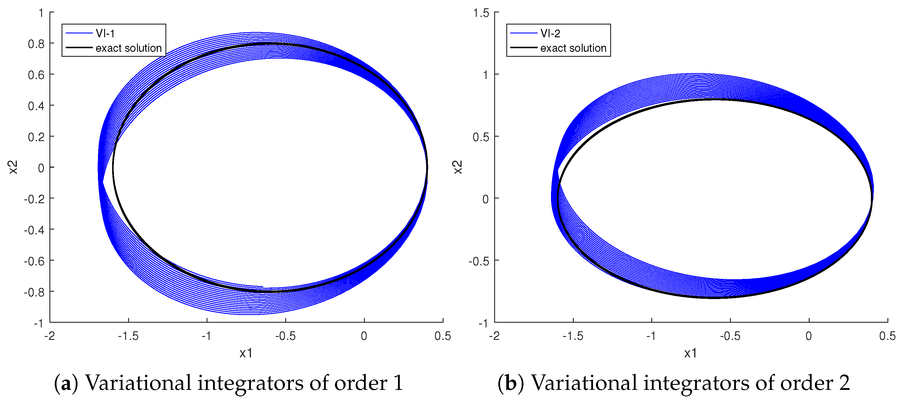
Using the initial conditions $(x_0,p_0)=(1-e,0;0,\sqrt{(1+e)/(1-e)})$ with $e=0.6$, and a time step of $h=0.05$, we perform numerical computations over $t\in [0,200]$. For comparison, we also show results from the symplectic Euler method and Störmer–Verlet method. The numerical orbits computed by the four variational integrators are shown in Figure 2. The orbit in the top-left corner is generated using the symplectic Euler method, while the top-right orbit is computed using the Störmer–Verlet method. The bottom-left and bottom-right orbits are simulated by the first- and second-order variational integrators (VI-1) and (VI-2), respectively. The background dotted line represents the exact orbit. It is clear that the numerical orbits on the top show a pronounced clockwise drift, while the two variational integrators provide better simulation results. Among the four methods, the orbit computed by the second-order variational integrator (VI-2) exhibits the least numerical error.

Table 1. Solution errors for the Kepler problem at $T=1$.

Sym-Euler	VI-1	SV	VI-2	h
7.4778 × 10−1	4.0499 × 10−1	7.0725 × 10−2	1.7794 × 10−2	1/200
2.7034 × 10−1	1.0920 × 10−1	1.7950 × 10−2	4.4287 × 10−3	1/400
1.0674 × 10−1	2.8301 × 10−2	4.5075 × 10−3	1.1077 × 10−3	1/800
4.6291 × 10−2	7.3240 × 10−3	1.1286 × 10−3	2.7721 × 10−4	1/1600
2.1409 × 10−2	1.9422 × 10−3	2.8229 × 10−4	6.9351 × 10−5	1/3200

compares solution errors. The variational integrators show smaller errors than classical methods of the same order.

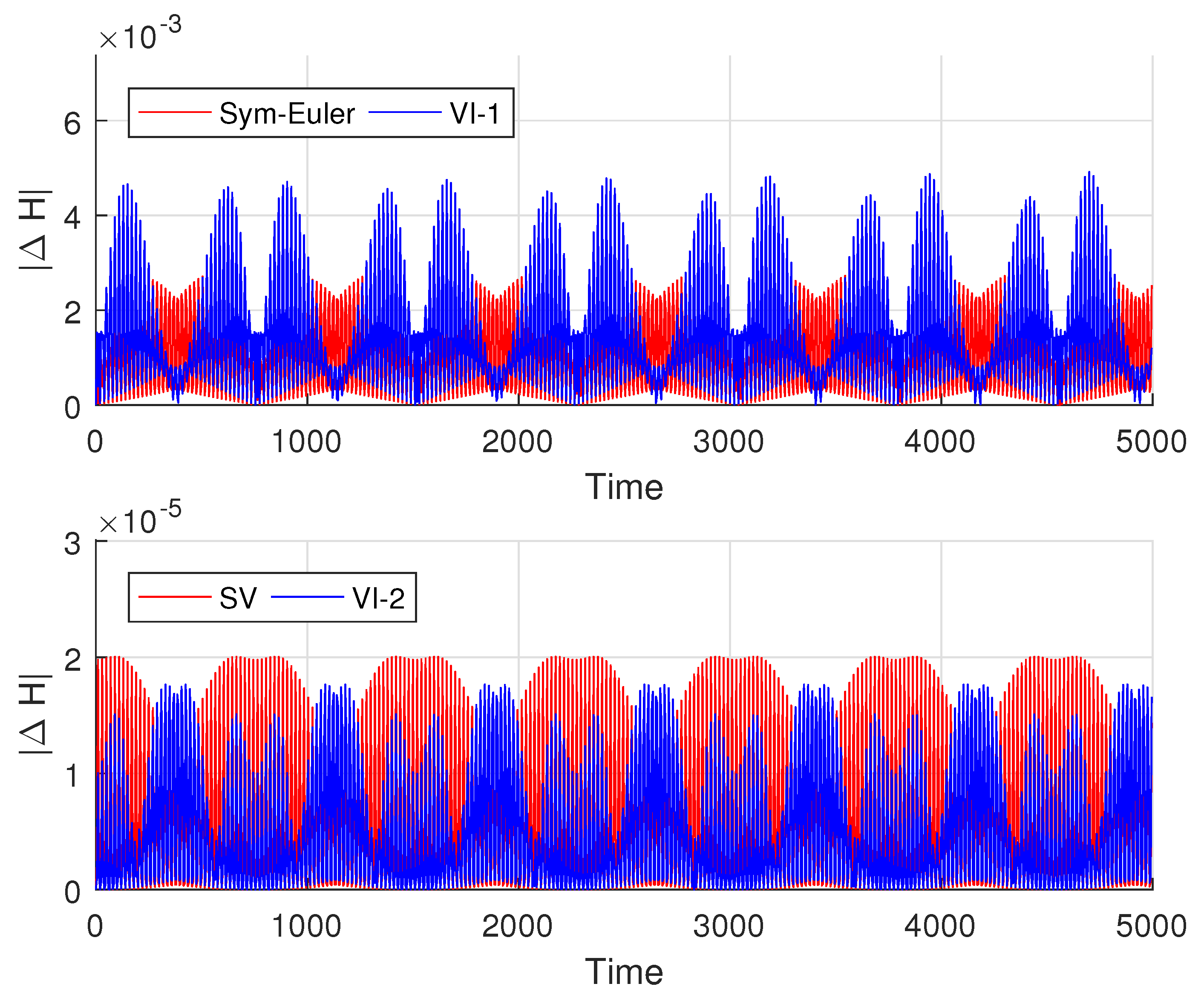
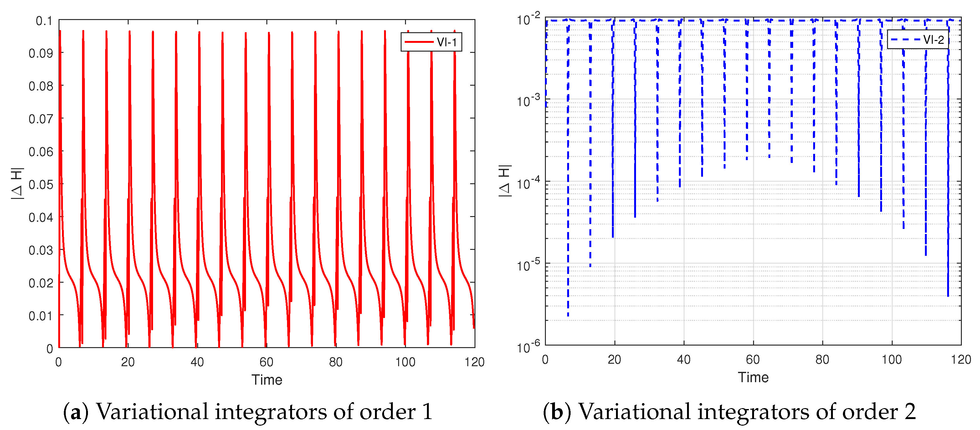
We now show the preservation of conservative quantities by the variational integrators. The initial conditions are $(x_0,p_0)=(-3,0;0,0.45)$, and the step size is $h=0.05$. From Figure 3, we observe that the numerical errors in energy can be bounded by all four variational integrators over the long term. For the Kepler system, the LRL vector defines the orientation and shape of the orbit. We present the numerical results for both the norm of the vector (eccentricity) and the angle (which governs the orientation and shape of the elliptical orbit). As discussed in Section 4, the solution of the variational integrator corresponds to the exact solution of the modified second-order differential equation. While the original Kepler system is super-integrable, the modified system is not. However, through backward error analysis [21,23], we show that the modified system remains integrable under symplectic methods. Thus, all four numerical methods bound the energy and momentum. The energy errors for the four variational integrators are plotted in Figure 3.

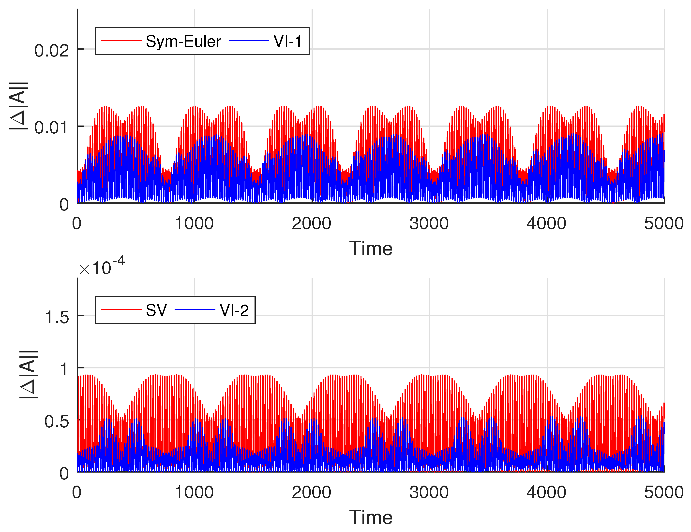
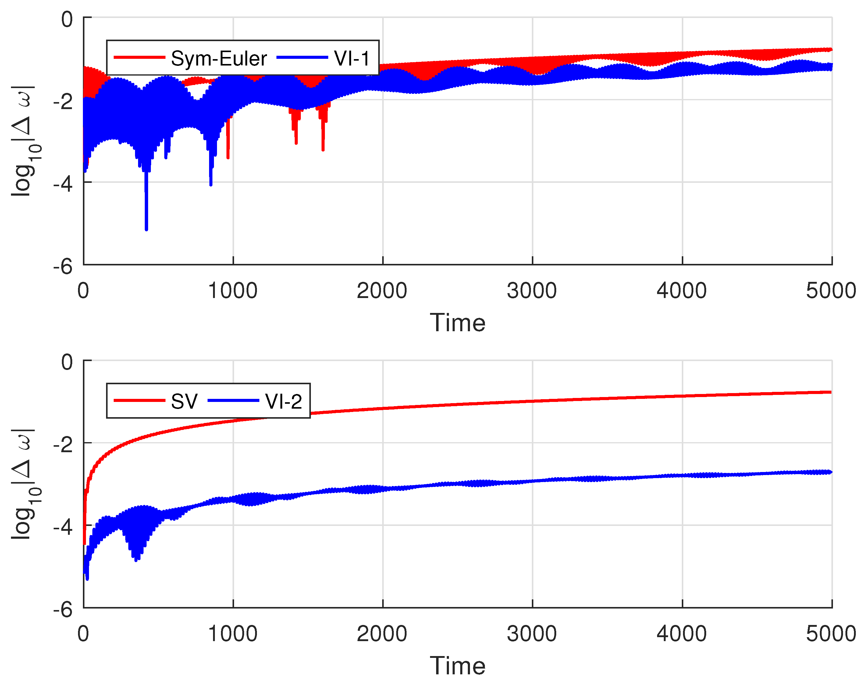
In Figure 4 and Figure 5, we compute the LRL vector using all four variational integrators. These figures show that the eccentricity error is bounded by all four methods, with the new variational integrators producing significantly smaller errors in both eccentricity and rotation angle.

We also present the convergence rates for the eccentricity and angle of the LRL vector, illustrated in Figure 6. To estimate the convergence order, we begin with $h=0.5$ and compute results for time steps $h_i=2^{-i}$, for $i=1,\dots ,6$. The results are shown in a log–log plot. For the eccentricity error in Figure 6a, both the symplectic Euler method and the first-order variational integrator exhibit second-order convergence. Their error curves are nearly identical. The Störmer–Verlet method shows super-convergence of order 4, while the second-order variational integrator also demonstrates super-convergence and produces smaller errors compared to the Störmer–Verlet method. In Figure 6b, we show the convergence rate for the angle error. All four methods exhibit a second-order convergence rate, consistent with the theoretical estimates in Section 4. The error curves for the symplectic Euler and Störmer–Verlet methods are nearly identical, but both the first- and second-order variational integrators show smaller errors in preserving the angle of the LRL vector. Among all four methods, the second-order variational integrator achieves the smallest errors, demonstrating superior performance.

• Relativistic Kepler system. This describes the motion of particles or bodies whose velocities are close to the speed of light. This system can be formulated by introducing proper time, with the Lagrangian given by $L(t,x;\gamma ,u)=-{\displaystyle \frac{1}{2}}{c}^2{\gamma }^2+{\displaystyle \frac{1}{2}}{u}^2+{\displaystyle \frac{\gamma }{\left|x\right|}}$. With scaled light speed $c={10}^2$, initial conditions $(x_0,p_0)=(0.4,0;0,2)$, and time step $h=0.05$ over $t\in [0,40]$, Figure 7 shows orbits computed by variational integrators (36) and (21). The mass shell $H(\gamma ,u)=-{\displaystyle \frac{c^2}{2}}{\gamma }^2+{\displaystyle \frac{1}{2}}{u}^2$ is the key conserved quantity. Figure 8 presents its error over 2500 steps. Both orbital trajectories and mass shell errors demonstrate good qualitative agreement, confirming the structure-preserving properties of the proposed methods in relativistic spacetime.

6. Concluding Remarks

In this paper, we consider a class of second-order systems in the form of (1) which model important physical systems, including classical mechanics and relativistic plasma dynamics. We have established the necessary and sufficient conditions for this class of second-order systems (1) to admit a variational formulation. These conditions relate to the geometric structures and conservative properties inherent in the given system. Our main contributions include constructing structure-preserving variational integrators through Lagrangian splitting, proving the equivalence of the newly derived variational integrators to explicit symplectic compositions, and demonstrating their superior performance using the Kepler problem as an example. We have also established the theoretical analysis by presenting modified Lagrangians for our newly derived variational integrators. Specifically, we have provided the recursive formula for the Nyström method. The numerical error estimates for conservative quantities, especially for the LRL vector, have been employed to verify the numerical superiority of the newly derived methods over classical numerical methods.

The variational framework developed in this paper can also be applied to simulate and analyse dynamical behaviour in astrophysical systems and relativistic dynamics. Furthermore, future work could extend to partial differential equations. For example, consider a non-linear wave equation with rotational symmetry and travelling wave solutions $u(t,x)=R\left(t\right)q(x-ct)$, where $R\left(t\right)=e^{at{J}^{-1}}$ and $J=\left[\begin{array}{cc}0& -1\\ 1& 0\end{array}\right]$. This reduction yields

$$(c^2-1)\ddot{q}=2ca{J}^{-1}\dot{q}+\left(a^2+V^{\prime }{\left(\right|q|}^2)\right)q.$$

As this system satisfies conditions (10) and (11), it admits a variational formulation when $c\ne 1$.