A Spatiotemporal Convolutional Neural Network Model Based on Dual Attention Mechanism for Passenger Flow Prediction

Abstract

Establishing a high-precision passenger flow prediction model is a critical and complex task for the optimization of urban rail transit systems. With the development of artificial intelligence technology, the data-driven technology has been widely studied in the intelligent transportation system. In this study, a neural network model based on the data-driven technology is established for the prediction of passenger flow in multiple urban rail transit stations to enable smart perception for optimizing urban railway transportation. The integration of network units with different specialities in the proposed model allows the network to capture passenger flow data, temporal correlation, spatial correlation, and spatiotemporal correlation with the dual attention mechanism, further improving the prediction accuracy. Experiments based on the actual passenger flow data of Beijing Metro Line 13 are conducted to compare the prediction performance of the proposed data-driven model with the other baseline models. The experimental results demonstrate that the proposed prediction model achieves lower MAE and RMSE in passenger flow prediction, and its fitted curve more closely aligns with the actual passenger flow data. This demonstrates the model’s practical potential to enhance intelligent transportation system management through more accurate passenger flow forecasting.

1. Introduction

Amidst growing demands and expanding scale in urban transportation, metro systems have become increasingly vital components of public transit infrastructure, particularly within major metropolitan areas [1,2]. Accurate passenger flow forecasting is a critical prerequisite for efficient and safe metro operations, constituting a prominent research focus with sustained scholarly attention. Robust forecasting capabilities are indispensable for optimizing resource allocation, enhancing service quality, and managing network congestion [3,4]. From the operator’s perspective, understanding passenger demand and traffic distribution patterns in complex metro networks are essential for maintaining service reliability and provides strong support for developing effective fault response strategies and safety and security [5,6]. In terms of train scheduling adjustment, accurate forecasting is also the basis of train adjustment strategy [7,8].

The actual passenger flow not only varies over time but is also influenced by various external factors and is a time function with a high degree of nonlinearity. The passenger flow distribution exhibits stochasticity and seems to fluctuate in both the temporal and spatial domains [9,10], and all these characteristics increase the difficulty of passenger flow forecasting.

With the widespread deployment of automated fare collection (AFC) devices in rail transit systems, operators have access to accurate passenger travel intelligent card data, enabling the construction of large databases that include station inbound and outbound passenger volumes and station origin–destination matrices [11,12,13], which provides the basis for passenger flow forecasting efforts. Currently, prediction models for passenger flow are mainly classified as parametric and nonparametric. The presence of an assumed functional correlation between the independent and dependent variables is defined as a parametric technique; in contrast, the absence of a correlation is defined as a nonparametric technique [14,15,16]. The emergence of nonparametric techniques has solved the limited capture of nonlinear relational structures. Neural networks have attracted much attention as representatives of nonparametric methods exhibit excellent mapping ability on arbitrary functions while generalizing extremely well [17]. However, traditional neural network models cannot handle the passenger flow data with high-dimensional, spatiotemporal characteristics. Further research has been prompted to improve neural networks to adapt to passenger flow data to achieve better predictions.

Based on the above discussion, the research of this study is to design a deep learning-based network architecture to improve its capability in processing high-dimensional and spatiotemporal characteristic data to achieve robust prediction of urban rail train passenger flow. The contribution of this paper is mainly in two aspects:

• A comprehensive study of two types of features was conducted to achieve simultaneous forecasting of multi-site passenger flow data. The two types of features include: (a) Temporal features of passenger flow time-series data, and (b) spatial features based on metro inter-station connections and passenger travel networks.
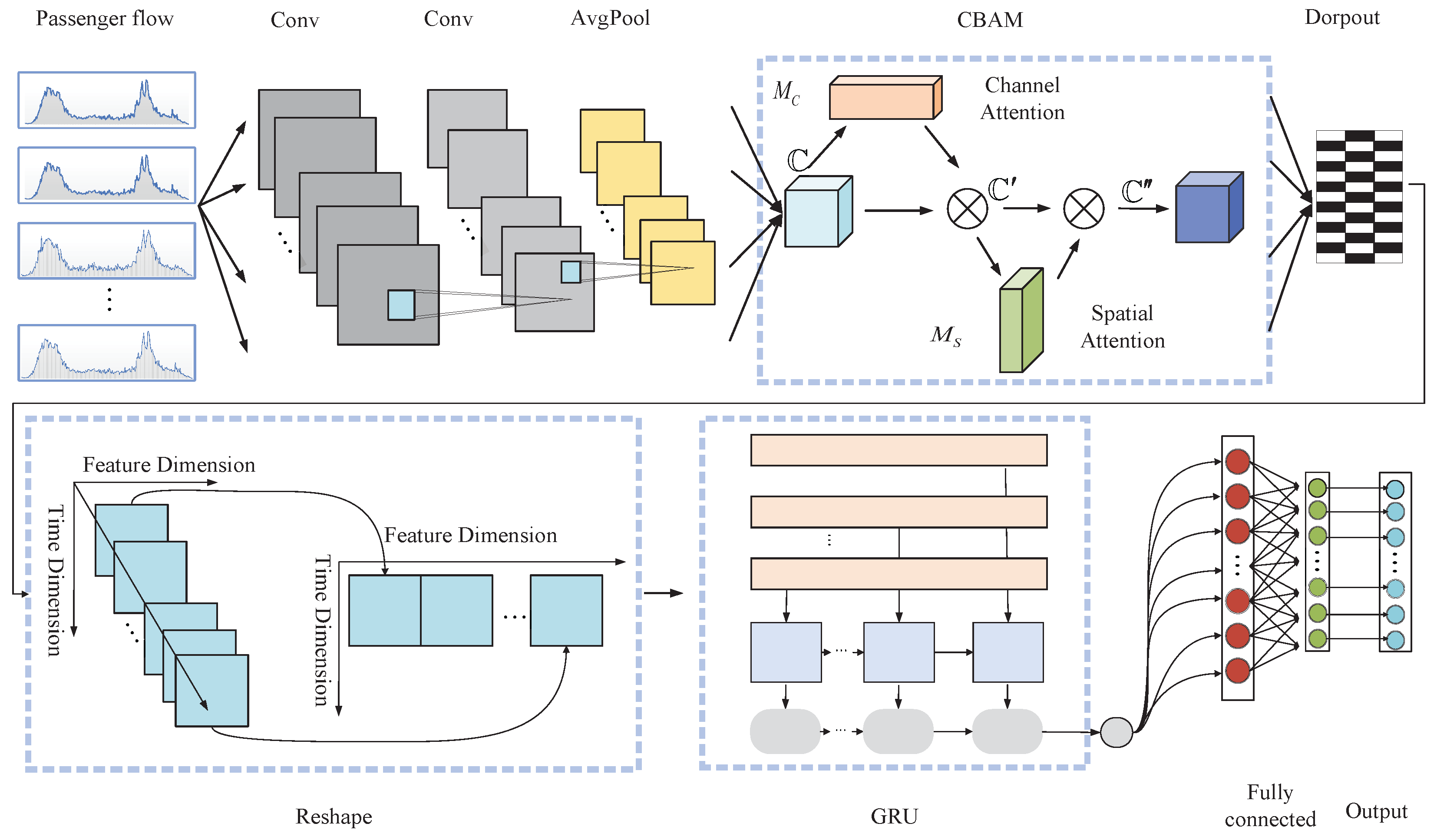
• A spatiotemporal convolutional network (GDAM-CNN) model with a dual attention mechanism is proposed, where a convolutional neural network (CNN) embedded with a convolutional block attention module (CBAM) is fused with a gated recursive unit (GRU) network to achieve effective capture of spatiotemporal features in passenger flow data. The GDAM-CNN model significantly enhances prediction accuracy by dynamically filtering critical spatial patterns through attention mechanisms (CBAM) while adaptively modeling temporal dependencies via gated recurrent units (GRU). This unified architecture jointly optimizes complex nonlinear spatiotemporal relationships.

The rest of this paper is organized as follows. In Section 2, recent work related to this topic is reviewed. In Section 3, the problem to be addressed in this study is described, followed by a detailed description of the various submodules of the GDAM-CNN model. In Section 4, experiments are first conducted to determine the parameters of the GDAM-CNN model, followed by the introduction of the baseline model and the inter-model analysis based on actual passenger flow and operational data of the Beijing subway lines. In Section 5, the work of this paper is summarized and future work is presented.

2. Literature Review

2.1. Traditional Statistical Methods

Over the last decades, passenger flow forecasting has been extensively studied. In the beginning years, the research was mainly focused on linear prediction with parameters, and various classical linear prediction models based on statistical theory were proposed in the same period. Among the parametric models, Cao et al. used an autoregressive sliding average model (ARMA) to build a prediction model of passenger flow, calculate the model’s parameters using the matrix method, and finally validate the model using field data [18]. Smith et al. used a historical averaging (HA) approach for traffic flow modeling based on the periodic nature of traffic flow, and reasonable estimation of historical data [19]. Williams et al. systematically investigated periodic temporal sequence modeling frameworks for univariate traffic volume prediction across urban expressway segments, ultimately establishing station-specific optimized seasonal adjustment methodology [20]. The Kalman filter (KF) has also been widely used in short-term traffic flow prediction problems. Jiao et al. introduced historical prediction errors into the measurement equation and developed an improved Kalman filter model for rail traffic flow prediction based on the error correction coefficient [21]. Shekhar et al. empirically validated the computational reliability and operational consistency of cyclical temporal analysis architectures integrated within adaptive signal refinement methodologies [22]. Okutani et al. proposed two short-term traffic volume prediction models using Kalman filter theory [23].

2.2. Nonparametric & Heuristic Models

Although the methods above perform well and robustly in modeling linear time series of relationships, this limits the application of the models to nonlinear relationship structures due to the assumption of linearity in the relationships between time-lagged variables. Later studies introduced nonparametric models to improve the ability of the model to capture nonlinear relationships. Representative nonparametric methods are nonparametric regression (NR), Gaussian maximum likelihood (GML), neural networks (NN), and other methods. The NR is a data-driven heuristic forecasting technique, which Yakowitz pioneered and Karlsson et al. have since applied to traffic flow forecasting [24,25]. Oswald et al. developed a passenger flow forecasting model applying an NR approach using advanced data structures and inexact calculations to reduce execution time [26]. Clark et al. proposed an intuitive method for generating passenger flow forecasts using pattern matching techniques using a multivariate expansion of the NR to exploit the three-dimensional nature of the flow states [27]. Kindzerske et al. proposed an integrated method of the NR for predicting traffic conditions [28]. Tang et al. used the GML method in a comparative study with other ways to develop a model for short-term forecasting of daily, weekly, and monthly passenger traffic [29].

2.3. Classical Neural Networks

Neural networks have developed rapidly in recent years. Neural networks can handle complex nonlinear problems without the need for a priori knowledge to define relationships between the input and output variables, and much research has been devoted to using neural network methods to solve traffic flow-related forecasting problems. Van et al. used multilayer perceptron neural networks to manage traffic flow, vehicles, and traffic demand based on data representing current and near-expected traffic conditions [30]. Zhang et al. developed an autoregressive traffic volume forecasting architecture employing temporal-delay neural networks (TDNNs), where the system identification process incorporates phase-space reconstruction of traffic fluctuation propagation patterns, with model dimension optimization achieved through temporal correlation metrics [31]. The object-oriented time-lag recurrent network (TLRN) short-term traffic flow prediction method was designed and implemented by Dia et al. [32]. Zheng et al. applied radial basis function neural networks to traffic flow prediction across temporal intervals, implementing an adaptive credit assignment heuristic algorithm rooted in Bayesian conditional probability principles. [33]. Chen et al. employed dynamic neural architectures for immediate-interval traffic volume forecasting, experimentally validating the framework’s operational viability through systematic analysis of traffic pattern datasets. [34]. Van et al. used state-space neural networks for accurate highway travel time prediction under missing data [35].

2.4. Deep Neural Networks

With the development of big data, deep learning has been widely studied. Deep learning models can better handle high-dimensional uncertain data and perform more efficiently and robustly than external neural networks in prediction problems. Because of the spatial and temporal characteristics of traffic flow data, the standard deep learning models used for traffic flow prediction are the recurrent neural networks (RNN), CNN, and their variants. Belhadi et al. proposed an RNN method called RNN-LF to predict long-term traffic flow from multiple data sources [36]. Li et al. designed an RNN-based short-term traffic flow prediction model. In this model, they used three different RNN structural units for model construction, and training [37]. Fu et al. used a long short-term memory (LSTM) and gated recurrent unit (GRU) neural network approach to predict short-term traffic flows [38]. The CNN is excellent at capturing spatial features. Zhang et al. determined the optimal input time lag and spatial data volume by the spatiotemporal feature selection algorithm (STFSA). The CNN learns these features to build the prediction model [39]. Spatio-temporal capture is difficult to achieve simultaneously using a single model, and some studies have combined the CNN with the RNN unit and their variants [40,41]. Using hybrid models to solve practical prediction problems has become a new research direction.

2.5. Attention-Based Deep Models

After that, attention mechanisms have been widely used in the field of traffic flow prediction to improve the ability of deep learning to pay attention to the main influencing factors and to increase the model’s perception of global spatiotemporal features to different degrees. Zhang et al. used the attention mechanism in combination with the LSTM units to jointly capture time-series information features [42]. Bai et al. proposed an attentional temporal graph convolutional network (A3T-GCN) to capture both global temporal dynamics and spatial correlation in traffic flow; an attentional mechanism (AM) is applied to adjust the importance of different time points, and pool global temporal information [43]. However, in the existing hybrid models based on attention mechanisms, the attention mechanisms are simply added for weight scoring, and there is no distinction and refinement of the attention mechanisms according to the models’ characteristics. In recent years, Woo et al. proposed the CBAM by combining spatial attention and channel attention [44], to achieve both the “what” and the “where” of engagement. Since then, the CBAM combined with the CNN has been widely used in image recognition research [45,46].

To sum up,

Table 1. Comparison of passenger flow forecasting methods.

Category	Representative Models	Strengths	Limitations
Traditional Statistical	ARMA (Cao et al. [18]), Kalman Filter (Okutani et al. [23])	Interpretable parameters; Computational efficiency	Linear assumption; Poor nonlinear fitting
Nonparametric & Heuristic	NR (Clark et al. [27]), GML (Tang et al. [29])	Data-driven; Handles nonlinearity	High computational cost; Overfitting risk
Classical Neural Networks	TDNN (Zhang et al. [31]), TLRN (Dia et al. [32])	Nonlinear mapping; Feature learning	Shallow architectures; Manual feature engineering
Deep neural networks	LSTM (Fu et al. [38]), CNN (Zhang et al. [39])	Automatic feature extraction; Spatiotemporal modeling	Black-box nature; Hardware-intensive
Attention-Based Deep	A3T-GCN (Bai et al. [43])	Dynamic feature weighting; Global context capture	Heuristic attention design; Untailored mechanisms

is a comparative table that summarizes the major models cited along with their key strengths and limitations.

3. Methods

In this subsection, the definition of the problem to be solved is first performed, followed by a detailed description of the GDAM-CNN model building process.

3.1. Definition of Problems

Define the variable ${\xi }_t^i$ to denote the ridership data at station i at moment t. The mapping relationship between the ridership data at the previous n moments and the passenger flow data at the next moment can be represented as:

$$\begin{array}{c}\hfill \left[\begin{array}{c}{\xi }_{t+1}^1\\ {\xi }_{t+1}^2\\ ⋮\\ {\xi }_{t+1}^{i-1}\\ {\xi }_{t+1}^i\end{array}\right]=\mu \left[\begin{array}{ccccc}{\xi }_{t-n}^1& {\xi }_{t-n+1}^1& \dots & {\xi }_{t-1}^1& {\xi }_t^1\\ {\xi }_{t-n}^2& {\xi }_{t-n+1}^2& \dots & {\xi }_{t-1}^2& {\xi }_t^2\\ ⋮& ⋮& \ddots & ⋮& ⋮\\ {\xi }_{t-n}^{i-1}& {\xi }_{t-n+1}^{i-1}& \dots & {\xi }_{t-1}^{i-1}& {\xi }_t^{i-1}\\ {\xi }_{t-n}^i& {\xi }_{t-n+1}^i& \dots & {\xi }_{t-1}^i& {\xi }_t^i\end{array}\right],\end{array}$$

(1)

where $\mu$ denotes the GDAM-CNN model, and it is worth emphasizing that i stations are on the same line, and the neighboring numbered stations are geographically adjacent to each other. In the matrix framework, horizontal dimensions shows that the passenger flow prediction relies on historical data, which is a time series problem; vertical dimensions describes the passenger flow relationship between different stations, which enhances the spatial relevance of the model prediction. Therefore, the regression of $\mu$ enables the dual capture of the spatial and temporal dimensions of passenger flow data.

3.2. Model Construction

The core challenge in metro passenger flow prediction lies in capturing nonlinear spatiotemporal dependencies across interconnected stations. To address these challenges, our framework integrates three specialized modules: The CBAM unit amplifies salient spatiotemporal features while suppressing noise through dual attention gates (Section 3.2.1); the CNN model extracts localized spatial features from station topology using grid convolution kernels (Section 3.2.2); and the GRU model temporal state transitions with gated memory cells handle dependencies (Section 3.2.3). This synergistic design enables hierarchical learning: spatial features from the CNN provide contextual inputs to the CBAM’s attention weighting, while the GRU recursively integrates temporal dynamics. The following sections formalize each module’s implementation. In this subsection, the CNN model, the CBAM unit, and the GRU model are introduced, and finally, the specific architecture of the GDAM-CNN model is given.

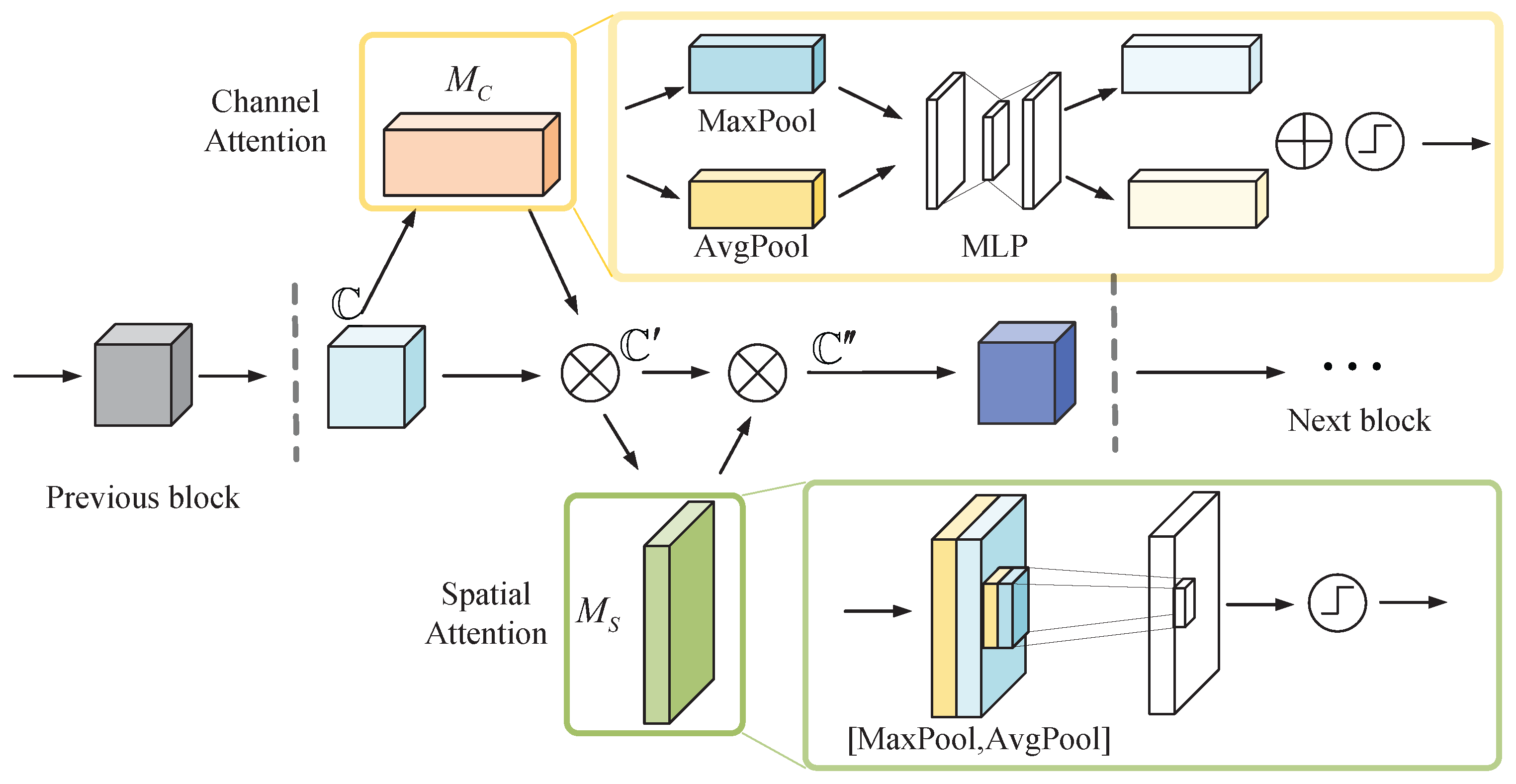
3.2.1. The CBAM Unit

The CBAM unit addresses feature saliency imbalance by dual attention gates that prioritize critical stations/time periods. The CBAM is a typical module based on the AM, which sequentially infers the attention information of the input features sequentially along two different dimensions: channel and space. It can not only increase the attention of the network to the critical elements but also suppress unnecessary features and increase the information flow weight of important features in the network.

In the channel attention part, the CBAM unit generates channel attention information using the inter-channel relationships between features. The spatial dimension of the input feature mapping is first compressed using average pooling and maximum pooling to improve channel attention computation efficiency. After that, the descriptors generated by the two pooling elements are forwarded to a shared network consisting of a multi-layer perceptron (MLP), and finally, the output feature information is merged by setting the reduction ratio to generate the channel attention. Given an intermediate feature information $\mathbb{C}\in {\mathbb{R}}^{C\times H\times W}$ as input, where C, H and W are the sizes of each dimension of the input feature. The transformation of feature information follows the following equation:

$$\begin{array}{c}\hfill \begin{array}{c}\hfill \begin{array}{c}\hfill M_C\left(\mathbb{C}\right)=\sigma (W_b\left(W_a\left({\mathbb{C}}_{avg}^c\right)\right)+W_b\left(W_a\left({\mathbb{C}}_{max}^c\right)\right)),\end{array}\end{array}\end{array}$$

(2)

where $M_C\left(\mathbb{C}\right)\in {\mathbb{R}}^{C\times 1\times 1}$ denotes the channel attention map output, $\mathrm{\Pi }$ indicates the changes that occur when the descriptors passes through the fully connected layer in the MLP, $\sigma$ denotes the sigmoid function, ${\mathbb{C}}_{avg}^c$ and ${\mathbb{C}}_{max}^c$ denote average-pooled features and max-pooled features, respectively, $W_a\in {\mathbb{R}}^{C/\phantom{Cr}r\times C}$ and $W_b\in {\mathbb{R}}^{C\times C/\phantom{\times Cr}r}$ are the weights of the shared network, and r denotes the reduction ratio.

The spatial attention is cascaded after the channel attention, and applies the convolutional layer to generate the spatial attention information. The spatial awareness not only achieves improved engagement with the focused information but also performs the labeling of the suppressed information. The spatial attention output $M_S\left(\mathbb{C}\right)\in {\mathbb{R}}^{1\times H\times W}$ can be expressed as follows:

$$\begin{array}{c}\hfill \begin{array}{c}\hfill \begin{array}{c}\hfill M_S\left(\mathbb{C}\right)=\sigma \left(f^{h\times w}\left([{\mathbb{C}}_{avg}^s;{\mathbb{C}}_{max}^s]\right)\right),\end{array}\end{array}\end{array}$$

(3)

where $\sigma$ denotes the sigmoid function, $f^{h\times w}$ denotes the convolution using a filter of size $h\times w$ for the convolution operation, ${\mathbb{C}}_{avg}^s$ and ${\mathbb{C}}_{max}^s$ denote average-pooled features and max-pooled features, respectively. The size of the filter we use in the CBAM is $5\times 5$.

In summary, the attention of the CBAM unit is summarized as follows:

$$\begin{array}{c}\hfill \begin{array}{c}\hfill {\mathbb{C}}^{\prime }=M_C\left(\mathbb{C}\right)\otimes \mathbb{C},\end{array}\end{array}$$

(4)

$$\begin{array}{c}\hfill \begin{array}{c}\hfill {\mathbb{C}}^{″}=M_S\left({\mathbb{C}}^{\prime }\right)\otimes {\mathbb{C}}^{\prime },\end{array}\end{array}$$

(5)

where ⊗ represents the corresponding multiplication of each element, ${\mathbb{C}}^{\prime }$ denotes the channel attention output, and ${\mathbb{C}}^{″}$ is the final output. The architecture diagram of the CBAM unit is as shown in Figure 1.

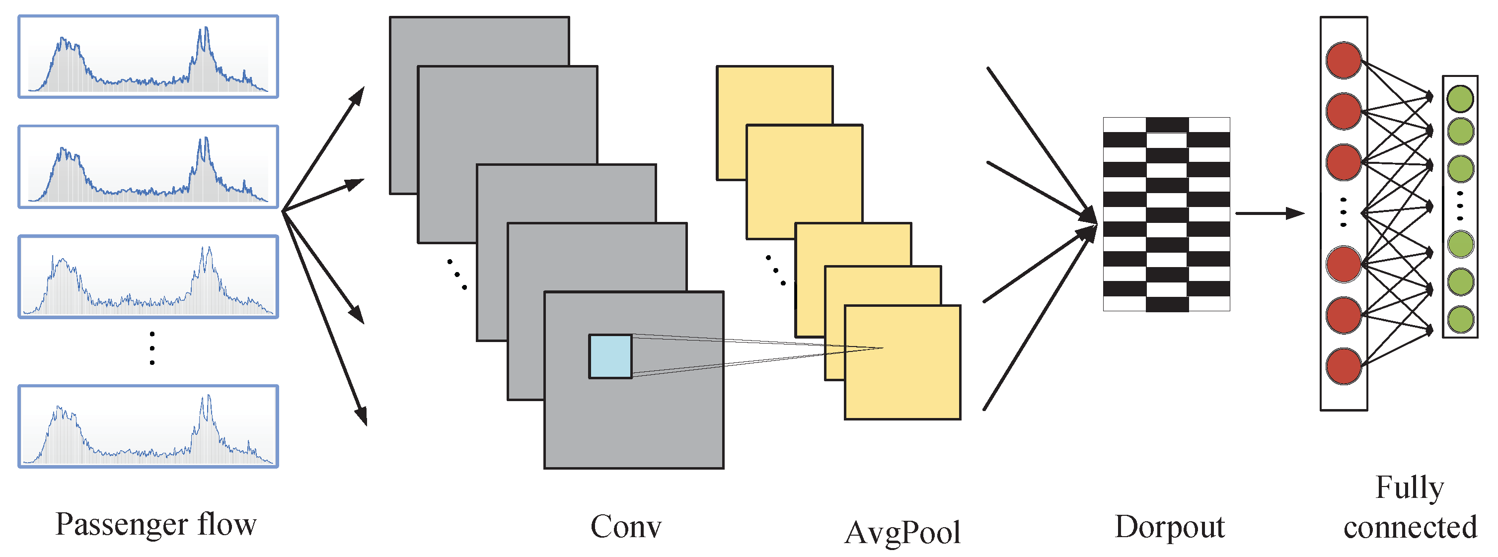
3.2.2. The CNN Model

Convolutional layers capture spatial relationships between adjacent stations using pattern-recognition filters that preserve station connectivity. The CNN consists of three main network layers: convolutional, pooling, and fully connected. The task of the convolutional and pooling layers is to filter the input data and extract useful information, which is usually used as input on the fully connected layer. The structure diagram of the CNN is shown in Figure 2.

The convolution layer applies a convolution operation between the original input data and the filter that generates the new feature values. The original purpose of this technique is to extract features from an image dataset, where the filter is a sliding window containing a matrix of coefficients that is “scanned” over the entire input matrix, and the process of “scanning” is a convolution operation with each subregion of the input matrix. The result of the convolution operation forms a new matrix representing the features specified by the applied filter, called convolutional features. Convolutional features are more descriptive of the data than the input matrix to improve the training efficiency, and usually, multiple filters are defined to perform different convolutional feature extraction. Convolution has one-dimensional, two-dimensional, and three-dimensional options. The purpose of our experiment is to extract the spatial features between data at a certain moment, and the input data can be approximated as a gray-scale map, so two-dimensional convolution is chosen here. We use $x_{p,q}^l$ to represent the input features at location $p,q$, and the convolution features at layer $lth$ can be mathematically represented as:

$$\begin{array}{c}\hfill \begin{array}{c}\hfill \begin{array}{cc}\hfill z_{p,q}^l=& x_{p,q}^l·w_{p,q}^l\hfill \\ \hfill =& {\sigma }^l\left({\displaystyle \sum _{s=-m}^m}{\displaystyle \sum _{t=-n}^n}{x}_{s,t}^l·w_{p-s,q-t}^l+b^l\right),\hfill \end{array}\end{array}\end{array}$$

(6)

where $w_{p,q}^l$ is the weight matrix, $b^l$ denotes the bias, the size of the $lth$ layer slice is $s,t$, and ${\sigma }^l$ denotes the sigmoid function used to enhance the characteristic nonlinearity at $lth$ layer. It is straightforward to see from the formula that the window size determined by the parameters m and n directly affects the result and time duration of the calculation and thus the model’s performance. The size of the sliding window determines the quality of feature extraction; too large a window will lose local feature information, and too small a window will reduce the correlation between local windows.

The purpose of the pooling layer is to reduce the dimensionality of the data and improve the overall computational efficiency. The features obtain after convolution are divided into equal regions. The components in this region are represented according to their maximum or average value and divided into two types: maximum pooling and average pooling. The maximum pooling is used in the experiment, and the maximum pooling at the $lth$ position $p,q$ can be mathematically represented as:

$$\begin{array}{c}\hfill \begin{array}{c}\hfill E_{p,q}^l=max(e_{1+h(p-1),1+h(q-1)}^{l-1},\dots ,e_{hp,h(q-1)}^{l-1},\dots ,e_{1+h(p-1),hq}^{l-1},\dots ,e_{hp,hq}^{l-1}),\end{array}\end{array}$$

(7)

where h denotes the local space region size $h\times h$.

After convolutional pooling, a dropout layer is usually added to prevent training overfitting. The data passing through the dropout layer is sent to the fully connected layer to participate in training other subsequent layers.

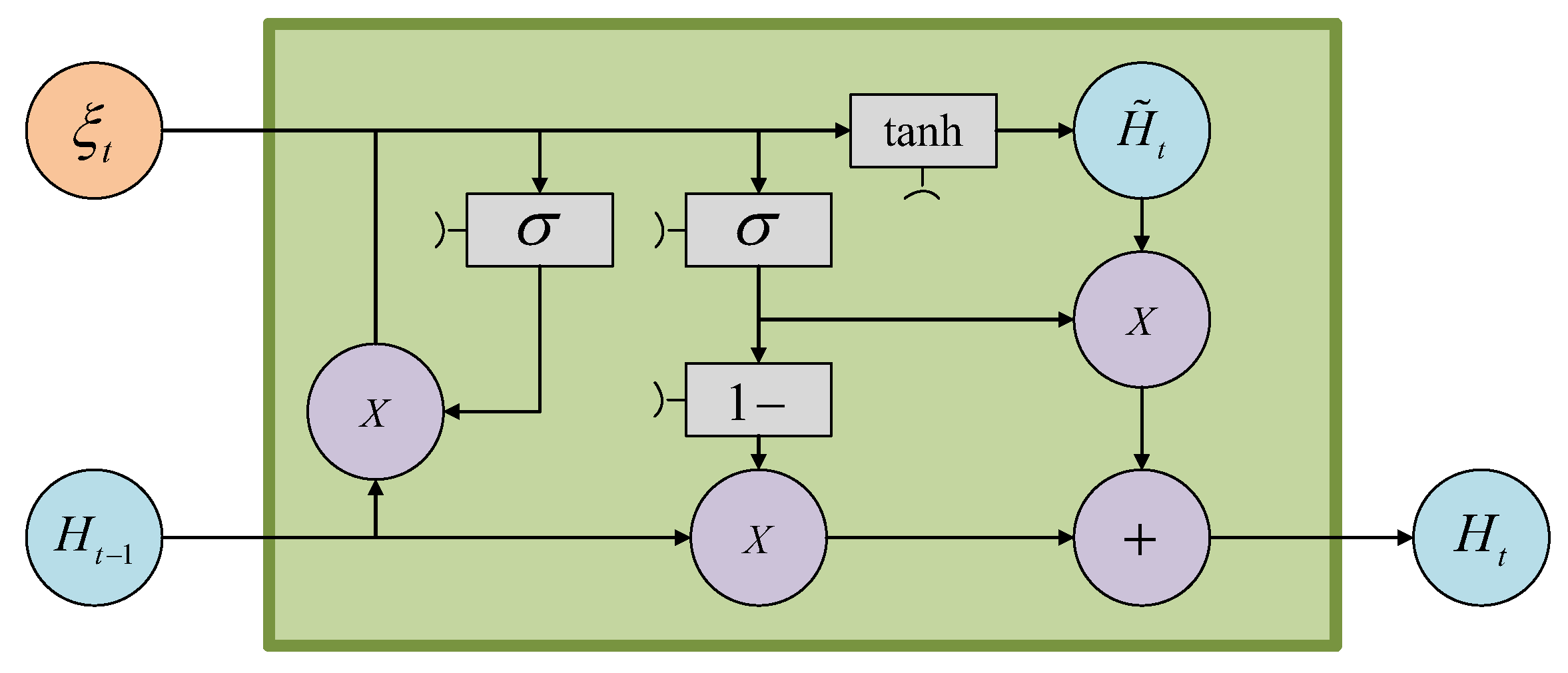
3.2.3. The GRU Model

The GRU’s gating mechanism maintains long-term periodicity while adapting to short-term disturbances via selective memory retention. The GRU is an excellent variant of the RNN that addresses the poor performance of feedforward neural networks on timing problems and improves the network’s ability to learn long-term dependencies by using feedback connection teaching to solve the gradient disappearance problem. Based on the connections shown in Figure 3, let $R_t$ denote the reset gate and $Z_t$ denote the update gate.

First, by concatenating the historical hidden state $H_{t-1}$ with the current input ${\xi }_t$ and applying the sigmoid activation function, the activation values of the reset gate $R_t$ and update gate $Z_t$ are computed. These gating parameters, distributed between 0 and 1, determine the intensity of information filtering. Subsequently, the gating reset operation is executed: performing element-wise multiplication between $R_t$ and $H_{t-1}$, followed by vector concatenation of the resulting product with the current input ${\xi }_t$. This composite signal is processed through the hyperbolic tangent activation function to generate the candidate hidden state ${\tilde{H}}_t$. This intermediate variable confines numerical values to the [−1, 1] interval via nonlinear transformation, with its core function being the encoding of feature information from the current input ${\xi }_t$, thereby providing short-term memory storage for subsequent state updates. During the memory update phase, the update gate $Z_t$ acts as a dynamic regulatory parameter, enabling adaptive renewal of the memory unit by controlling the linear weighted combination ratio between the historical state $H_{t-1}$ and the candidate state ${\tilde{H}}_t$. Specifically, when $Z_t$ approaches 1, the system prioritizes retaining historical information; when it approaches 0, it emphasizes the integration of new features from the current input. Ultimately, the hybrid state modulated by these gating parameters constitutes the new hidden state $H_t$ of the GRU unit. The above process is expressed using the following equation:

$$\begin{array}{c}\hfill \begin{array}{c}\hfill {\tilde{H}}_t=tanh(W_h{\xi }_t+Q_h(R_t\odot H_{t-1})+b_h),\end{array}\end{array}$$

(8)

$$\begin{array}{c}\hfill \begin{array}{c}\hfill H_t=(1-Z_t)\odot H_{t-1}+Z_t\odot {\tilde{H}}_t,\end{array}\end{array}$$

(9)

with the two gates presented as:

$$\begin{array}{c}\hfill \begin{array}{c}\hfill R_t=\sigma (W_r{\zeta }_t+Q_r{H}_{t-1}+b_r),\end{array}\end{array}$$

(10)

$$\begin{array}{c}\hfill \begin{array}{c}\hfill Z_t=\sigma (W_z{\xi }_t+Q_z{H}_{t-1}+b_z).\end{array}\end{array}$$

(11)

In the architectural parametrization, $W_r$, $W_z$, $W_h$, $Q_r$, $Q_z$, and $Q_h$ represent learnable parameter matrices governing reset gate dynamics, update gate operations and hidden state calculation, respectively, while $b_r$, $b_z$, $b_h$ denote corresponding offset parameters. The ⊙ denotes the scalar product of two vectors. Here, $\sigma \left(x\right)$ is the Sigmoid function defined as $\sigma \left(x\right)=\frac{1}{1+e^{-x}}$, and the tanh function is the hyperbolic sine function defined as $tanh\left(x\right)=\frac{e^x-e^{-x}}{e^x+e^{-x}}$.

3.2.4. The GDAM-CNN Model

We integrate three network units, the CNN, the CBAM, and the GRU, to form the GDAM-CNN network with dual attention and spatiotemporal feature capture capability. The CBAM units are first integrated into the CNN network, after determining the CBAM location as the output of each convolutional module. After that, it is connected to the reshape layer to downscale the data. In the CNN stage, we turn the original two-dimensional passenger flow data into three-dimensional after the slicing process, which needs to be downscaled to two-dimensional data to connect to the GRU smoothly afterward. At the same time, considering that the input sequence of the GRU needs to ensure the time delay information, we keep the time delay information in the conversion and merge the other two dimensions of feature information into one dimension. After the reshape layer, the GRU network unit is connected to give the network the ability to handle long-time sequences. The entire GDAM-CNN network structure is shown in Figure 4.

4. Experiment Results

In this subsection, we perform the presentation of the experimental results, starting with the processing of the field data used for the experiments before the start of the investigation, followed by the parameter determination session of the GDAM-CNN model, and finally, the description of the experimental situation in comparison with other baseline models.

4.1. Data Processing and Evaluation Metrics

In the experiment, we use the AFC’s actual passenger flow data. For each passenger’s one-way travel record, the integrated circuit (IC) card will generate two inbound and outbound records in the AFC system. Taking the inbound record as an example, the fields of the record include card ID, swipe time, swipe station, inbound status, card type, etc. For the experiment, we collect the passenger flow data in 16 subway stations from Xizhimen to Dongzhimen of Beijing Subway Line 13, and select the passenger flow data from 5:00 a.m. to 11:00 p.m. and collate them in 5-min intervals.

Remark 1.

This study focuses on passenger flow prediction for stations along individual metro lines, where all adjacent grids are geographically interconnected and exhibit flow interactions. For a single metro line or roadway, it can be treated as a one-dimensional grid [47]. For grid-structured data, convolutional neural networks are adequate for automatically extracting spatial features [48]. Within the metro network, the actual non-Euclidean distances and spatial dependencies of interconnectivity between stations are not explicitly defined, making graph-based models (such as graph convolutional networks and graph attention networks) more suitable for accurately characterizing spatial correlations.

The first step is to select the required field information from the numerous fields, which requires removing irrelevant information from the original dataset to obtain the data we need for further training. At the same time, we note that the data are taken in inconsistent or even widely different ranges in our input data, which will lead to uneven distribution of model weights and affect the training effect. Therefore, the second step is that the data needs to be normalized before training to map the data within the range of 0 to 1. We define ${\mathrm{X}}_{it}$ to represent the passenger flow data to form a two-dimensional matrix, and the process of normalization using the maximum–minimum value can be expressed as:

$$\begin{array}{c}\hfill \begin{array}{c}\hfill {{\mathrm{X}}_{it}}^{*}=\frac{{\mathrm{X}}_{it}-min\left({\mathrm{X}}_{it}\right)}{max\left({\mathrm{X}}_{it}\right)-min\left({\mathrm{X}}_{it}\right)},\end{array}\end{array}$$

(12)

where ${{\mathrm{X}}_{it}}^{*}$ denotes the normalized value of ${\mathrm{X}}_{it}$, $max\left({\mathrm{X}}_{it}\right)$ and $min\left({\mathrm{X}}_{it}\right)$ represent the maximum and minimum values in the matrix, respectively.

To make the experimental results more accurate, we repeat each experiment 100 times due to the uncertainty of the neural network. Afterward, the mean and standard deviation of the metrics are obtained as the final experimental results. The metrics we use in the experimental process are mean absolute error (MAE) and root mean square error (RMSE). The metrics are defined as follows:

$$\begin{array}{c}\hfill \begin{array}{c}\hfill \mathrm{MAE}=\frac{1}{N}{\displaystyle \sum _{i=1}^N}\left|p_i-{\widehat{p}}_i\right|,\end{array}\end{array}$$

(13)

$$\begin{array}{c}\hfill \begin{array}{c}\hfill \mathrm{RMSE}=\sqrt{\frac{1}{N}{{\displaystyle \sum _{i=1}^N}\left(p_i-{\widehat{p}}_i\right)}^2},\end{array}\end{array}$$

(14)

where $p_i$ is the actual passenger flow data, ${\widehat{p}}_i$ is the predicted passenger flow data, and N is the total number of predicted passengers. The training environment for deep learning is particularly important; the environment and its version used in the experiment are as follows: Windows 10 system, GPU (GeForce GTX 1060), Python (3.6.0), Tensorflow (2.6.2), Numpy (1.19.5), and Keras (2.6.0).

4.2. Parameter Settings

For neural networks, the parameters of the model greatly determine the model’s performance, so it is necessary to conduct a series of experiments to select model parameters. The critical parameters for the GDAM-CNN model are the network depth of the CNN and the GRU, the number of filters in the convolutional unit, the number of neurons in the GRU hidden layer, and the step size of the prediction, etc.

First, we determine the number of layers of the CNN and the GRU units in the network. In general, as the number of layers of the neural network increases, the training effect will show from under-fitting to well-fitting to over-fitting, and the training time will gradually increase. Since the CNN and the GRU combine to affect the performance of the GDAM-CNN model, as well as to balance the experimental results and the experimental time cost, we set the number of layers of the two neural networks from 1 to 3 layers, respectively, to find the suitable combination of network layers by experimenting with real card traffic data. For neural networks, the network depth and the number of neurons in each layer are interdependent [49], so we set the number of neurons of both the CNN and the GRU networks as 64 in our experiments to determine the number of layers of the network. The experimental results are shown in

Table 2. Model performance with different layers.

MAE/RMSE	GRU	1	2	3
CNN
1		24.171 ± 0.616	24.694 ± 1.693	25.102 ± 2.193
		34.536 ± 0.501	34.714 ± 2.348	34.943 ± 2.379
2		23.938 ± 0.892	23.954 ± 0.757	24.579 ± 1.180
		34.095 ± 0.980	34.151 ± 0.972	34.588 ± 1.673
3		24.691 ± 1.040	26.919 ± 3.522	24.393 ± 1.165
		35.736 ± 1.412	38.989 ± 4.909	35.384 ± 1.741

. The table shows that the network performance is best when the number of layers of the CNN and the GRU units is set to 2 and 1, respectively.

The following experiment is to determine the number of neurons. Generally, the number of neurons in each neural network layer is usually 32, 64, 128, etc. In common variants of CNNs such as VGG-16, AlexNet, GoogleNet, etc., the number of neurons in the convolutional layer increases incrementally as the number of layers increases. Therefore, the number of neurons in the two-layer convolution is also set incrementally and combined with the number of GRU neurons to find the most suitable combination for the GDAM-CNN network.

Table 3. Model performance with different layers.

MAE/RMSE	CNN	32, 64	32, 128	64, 128
GRU
32		24.649 ± 0.819	24.372 ± 0.691	24.134 ± 0.677
		35.170 ± 1.970	34.028 ± 0.952	34.374 ± 1.261
64		24.707 ± 0.460	22.988 ± 0.682	25.312 ± 0.129
		35.0659 ± 0.658	33.194 ± 0.910	36.727 ± 0.489
128		24.761 ± 1.206	25.242 ± 0.328	24.477 ± 1.249
		36.077 ± 2.061	36.123 ± 0.461	34.362 ± 1.386

shows the metrics under various combinations. The network’s performance is best when the number of neurons in the two convolutional layers is 32 and 128, respectively, and the number of neurons in the GRU is 64.

Next, experiments on the effect of parameter n on the model’s accuracy are conducted. As described in Section 3.1, the GDAM-CNN model uses the passenger flow data of the previous n moments to predict the passenger flow data of the next moment, where the moment is the smallest discrete time unit of our data which is 5 min. We increase the value of n from 6 to 24 and conduct experiments using actual passenger flow data, and the experimental results are shown in

Table 4. Model performance for different values of the parameter n.

Step Size	MAE	RMSE
6	26.290 ± 2.747	38.222 ± 3.494
8	24.201 ± 1.041	35.291 ± 1.643
10	23.170 ± 0.794	33.363 ± 1.410
12	24.731 ± 1.376	35.526 ± 2.061
14	25.175 ± 1.193	36.272 ± 2.200
16	25.772 ± 1.969	36.116 ± 3.697
18	26.014 ± 1.608	37.021 ± 2.264
20	24.867 ± 1.316	35.707 ± 2.553
22	25.624 ± 1.407	36.111 ± 2.189
24	24.037 ± 1.435	34.967 ± 2.309

.

In general, within a specific range, the longer the step length, the more information about the state at the previous time can be obtained. However, the experimental results show that, the model’s performance with n values from 12 to 18 shows that too large a step size cannot significantly improve the model’s performance. Meanwhile, during the experiment, we find that as the step length increases, the information increases and the training duration of the model grows, so it is imperative to select the appropriate parameters according to the characteristics of the input data and the adaptive capacity of the model itself. Finally, we choose $n=10$ as the value of the step size of the model.

4.3. Performance of the GDAM-CNN Model

In this section, the GDAM-CNN model performance is compared with the prediction performance of other standard prediction models. For the choice of baseline models, the first baseline model uses a fully connected neural network (FCN); the second model is a CNN network; the third model is chosen as an LSTM network; the fourth model is chosen as a GRU network; after which to reflect the superiority of the GRU on time series, the fifth network we delete the GRU unit of the network and use a CNN, and a CBAM in sequential series, denoted by the CNN-CBAM; for the sixth network we use the GRU, and the CBAM in sequential tandem, denoted by the GRU-CBAM; for the last network to verify the ability of the CBAM to focus on the main features, a CNN-GRU network in tandem is used. The network units used in the experiments for each model and their corresponding number of neurons are shown in

Table 5. The model and its corresponding parameters.

Model	The Model Uses Network Units and the Number of Neurons
FCN	FCN (128)
CNN	CNN (32),CNN (128)
LSTM	LSTM (64), LSTM (64)
GRU	GRU (64), GRU (64)
CNN-CBAM	CNN (32), CNN (128), CBAM
GRU-CBAM	GRU (64), GRU (64), CBAM
CNN-GRU	CNN (32), CNN (128), GRU (64)
GDAM-CNN	CNN (32), CNN (128), CBAM, GRU (64)

.

The first step is to verify the stability of the GDAM-CNN model. We execute several iterations of the experiment and find that with the increase in the number of training rounds, it is always possible to stabilize the model loss after 20 iterations gradually. Additionally, it keeps fluctuating within a specific tolerance range in the subsequent training, as Figure 5 shows the convergence of the loss curve of the model. It indicates that the GDAM-CNN model is convergent and has specific stability.

To verify the advantages of the designed model in predicting passenger flow, we compare the GDAM-CNN model with seven benchmark deep learning models introduced earlier (FCN, CNN, LSTM, GRU, CNN-GRU, CNN-CBAM, GRU-CBAM) as well as traditional models (SARIMA and Random Walk), and other deep learning models (Informer, U-NET, StemGNN). The metrics of each model are presented in

Table 6. The comparison results of different methods.

Model	MAE	RMSE
FCN	33.26	46.22
CNN	27.45	40.83
LSTM	29.47	41.97
GRU	29.51	41.26
CNN-GRU	23.78	32.84
CNN-CBAM	25.06	36.11
GRU-CBAM	24.31	34.79
GDAM-CNN	16.71	22.09
SARIMA	41.25	64.13
Random-Walk	35.76	52.51
Informer	32.35	47.11
U-NET	29.94	40.87
StemGNN	30.10	43.15

.

The following conclusions can be drawn from the results:

• The FCN model predicts poorly because it cannot effectively capture the temporal correlation between the data.
• Because it can capture the temporal correlation between the data well, the performance of the LSTM and the GRU models improves compared to the FCN, and both implementations are close under the MAE metric. Still, the GRU performs better under the RMSE metric. Meanwhile, during the experiments, we find that the training time of the GRU is shorter with the same network parameters, because each GRU unit uses fewer gate parameters than the LSTM unit, so we choose to use the GRU instead of the LSTM.
• The comparison of the GRU, the GRU-CBAM, the CNN, and the CNN-CBAM shows that integrating the CBAM module in the model can significantly improve the model performance, which proves that the CBAM can improve the performance of the model by increasing the focus on the main influencing factors while suppressing the focus on unimportant information.
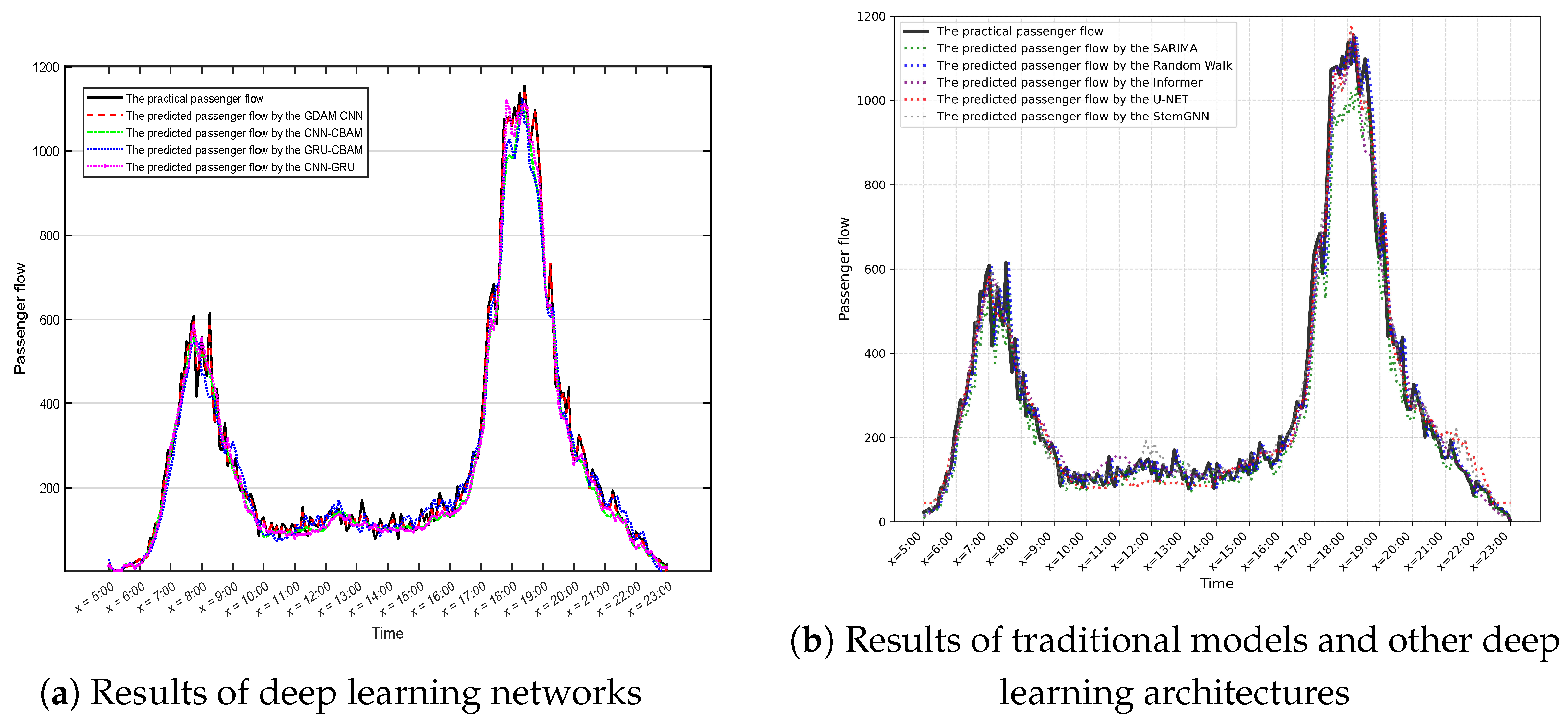
• The CNN-GRU model performs better because the CNN and the GRU units give the model the ability to capture the spatial and temporal correlation between the data.
• The GDAM-CNN model performs best by comparison because it can not only focus on the focused information but also capture the spatiotemporal correlation between data, which integrally improves the model’s prediction performance.
• Traditional models (ARIMA and Random Walk) exhibit higher MAE and RSE compared to deep learning approaches. As can be seen from the table, compared to the GDAM-CNN prediction model proposed in this paper, the ARIMA method exhibits a 148.9% increase in MAE and a 190.3% increase in RMSE. Similarly, although the Random Walk outperforms the ARIMA, it shows 114% higher MAE and 137.7% higher RMSE than the GDAM-CNN. From the above analysis, it can be observed that the two traditional prediction methods exhibit higher MAE and RSE compared to deep learning approaches. This is because the ARIMA, as a linear statistical model, and the Random Walk, which assumes constant variance, fail to adequately model the complex nonlinearities and spatiotemporal dynamics inherent in the passenger flow data.
• From the table, it can be observed that the prediction results of the U-Net-style architecture method show a 79.2% higher MAE and 85% higher RMSE compared to the GDAM-CNN, yet it remains the best performing model among the three selected models. Among other deep learning models, the U-Net-style architecture method benefits from its effective multi-scale feature extraction architecture. This enables it to capture important patterns at different resolutions, achieving performance levels comparable to established models like the CNN and the LSTM.
• Models based on the Transformer architecture (Informer and StemGNN) demonstrate performance variations. Specifically, StemGNN, which combines spectral graph convolution, captures spatiotemporal patterns to a degree that yields results close to several baseline deep models such as GRU. Informer also attempts to model long sequences but achieves results similar to the weaker FCN baseline, highlighting the challenge of effectively applying pure Transformer variants to this specific passenger flow prediction task. Their performance, while superior to traditional methods, remains inferior to models like the CNN-GRU and the GDAM-CNN that are specifically designed or enhanced for spatiotemporal feature focus.

Finally, we use the models to predict the passenger flow of the same station on the same day. For the sake of observation, we plot the prediction results in two comparative figures: Figure 6a displays the better performing models among the seven deep learning networks: the CNN-GRU, the CNN-CBAM, the GRU-CBAM, and the GDAM-CNN. Figure 6b includes the prediction curves of traditional statistical models (ARIMA and Random Walk) and other deep learning architectures (Informer, U-NET, StemGNN). By comparing the fitted curves in the figure, it can be observed that the training results of the ARIMA and the Random Walk are significantly underfit. The actual passenger flow exhibits extremely strong volatility, but the prediction results of these two traditional forecasting models fail to capture this characteristic. This further demonstrates the effectiveness of using deep learning methods for passenger flow prediction. Additionally, it can be observed that the curves produced by the three prediction models are similar and show a relatively close fit to the actual passenger flow data. However, they still fall slightly short compared to the GDAM-CNN model mentioned in this paper. It is clear from the predicted curves in Figure 6a that GDAM-CNN performs more prominently where the passenger flow changes are complex, indicating that CBAM is able to capture the main factors affecting the model.

5. Conclusions

This study explores the problem of predicting passenger flow in different urban rail transit stations. The proposed method is designed based on deep learning networks. Firstly, based on the traditional CNN network, the CBAM module is integrated to improve the model’s ability to focus on critical influencing factors and suppress the focus on non-important aspects to improve the prediction accuracy. Then the GRU units are added to capture the spatiotemporal correlation of data for the whole model together with the CNN network. Finally, simulation results based on actual passenger flow data are given to compare the prediction performance of the proposed model and other baseline models with the same data set. The results show that the proposed model exhibits significantly better performance under both the MAE and the RMSE metrics.

This study has limitations to address, and further research can be conducted to improve it. First, future work should incorporate factors such as weather, which can be considered in addition to the spatiotemporal dimensional characteristics of passenger flow. Second, we will continue to predict the passenger flow of each station line together with other lines to facilitate the integrated management of the passenger flow of each station line. Third, while the current model demonstrates strong predictive performance, its spatial modeling approach assumes grid-structured station relationships. Future research could investigate graph-based neural architectures (e.g., graph convolutional networks) to explicitly model non-Euclidean spatial dependencies, particularly for transfer stations where complex passenger flow patterns transcend simple adjacency relationships. Such approaches may yield additional improvements for metro networks with more complex topological structures.

References

1. Zhou, S.; Liu, H.; Wang, B.; Chen, B.; Zhou, Y.; Chang, W. Public Norms in the Operation Scheme of Urban Rail Transit Express Trains: The Case of the Beijing Changping Line. Sustainability 2021, 13, 7187. [Google Scholar] [CrossRef]
2. Song, H.; Gao, S.; Li, Y.; Liu, L.; Dong, H. Train-centric communication based autonomous train control system. IEEE Trans. Intell. Veh. 2023, 8, 721–731. [Google Scholar] [CrossRef]
3. Wang, W.W. Study on Forecast of Railway Passenger Flow Volume under Influence of High-speed Railways. Railw. Transp. Econ. 2016, 38, 42–46. [Google Scholar]
4. Sun, Y.; Leng, B.; Guan, W. A novel wavelet-SVM short-time passenger flow prediction in Beijing subway system. Neurocomputing 2015, 166, 109–121. [Google Scholar] [CrossRef]
5. Sun, L.; Lu, Y.; Jin, J.G.; Lee, D.H.; Axhausen, K.W. An integrated Bayesian approach for passenger flow assignment in metro networks. Transp. Res. Part C Emerg. Technol. 2015, 52, 116–131. [Google Scholar] [CrossRef]
6. Jing, Z.; Yin, X. Neural network-based prediction model for passenger flow in a large passenger station: An exploratory study. IEEE Access 2020, 8, 36876–36884. [Google Scholar] [CrossRef]
7. Wang, X.; Li, S.; Tang, T.; Yang, L. Event-triggered predictive control for automatic train regulation and passenger flow in metro rail systems. IEEE Trans. Intell. Transp. Syst. 2022, 23, 1782–1795. [Google Scholar] [CrossRef]
8. Wang, X.; Wei, Y.; Wang, H.; Lu, Q.; Dong, H. The dynamic merge control for virtual coupling trains based on prescribed performance control. IEEE Trans. Ind. Inform. 2025, 21, 4779–4788. [Google Scholar] [CrossRef]
9. Yin, J.; Tang, T.; Yang, L.; Gao, Z.; Ran, B. Energy-efficient metro train rescheduling with uncertain time-variant passenger demands: An approximate dynamic programming approach. Transp. Res. Part B Methodol. 2016, 91, 178–210. [Google Scholar] [CrossRef]
10. Song, H.; Xu, M.; Cheng, Y.; Zeng, X.; Dong, H. Dynamic Hierarchical Optimization for Train-to-Train Communication System. Mathematics 2025, 13, 50. [Google Scholar] [CrossRef]
11. Reddy, A.; Lu, A.; Kumar, S.; Bashmakov, V.; Rudenko, S. Entry-only automated fare-collection system data used to infer ridership, rider destinations, unlinked trips, and passenger miles. Transp. Res. Rec. 2009, 2110, 128–136. [Google Scholar] [CrossRef]
12. Song, H.; Li, L.; Li, Y.; Tan, L.; Dong, H. Functional Safety and Performance Analysis of Autonomous Route Management for Autonomous Train Control System. IEEE Trans. Intell. Transp. Syst. 2024, 25, 13291–13304. [Google Scholar] [CrossRef]
13. Wang, Z.; Gao, G.; Liu, X.; Lyu, W. Verification and Analysis of Traffic Evaluation Indicators in Urban Transportation System Planning Based on Multi-Source Data—A Case Study of Qingdao City, China. IEEE Access 2019, 7, 110103–110115. [Google Scholar] [CrossRef]
14. Bai, Y.; Sun, Z.; Zeng, B.; Deng, J.; Li, C. A multi-pattern deep fusion model for short-term bus passenger flow forecasting. Appl. Soft Comput. 2017, 58, 669–680. [Google Scholar] [CrossRef]
15. Wei, Y.; Chen, M.C. Forecasting the short-term metro passenger flow with empirical mode decomposition and neural networks. Transp. Res. Part C Emerg. Technol. 2012, 21, 148–162. [Google Scholar] [CrossRef]
16. Smith, B.L.; Williams, B.M.; Oswald, R.K. Comparison of parametric and nonparametric models for traffic flow forecasting. Transp. Res. Part C Emerg. Technol. 2002, 10, 303–321. [Google Scholar] [CrossRef]
17. Zhang, G.; Patuwo, B.E.; Hu, M.Y. Forecasting with artificial neural networks: The state of the art. Int. J. Forecast. 1998, 14, 35–62. [Google Scholar] [CrossRef]
18. Cao, L.; Liu, S.G.; Zeng, X.H.; He, P.; Yuan, Y. Passenger flow prediction based on particle filter optimization. Appl. Mech. Mater. 2013, 373–375, 1256–1260. [Google Scholar] [CrossRef]
19. Smith, B.L.; Demetsky, M.J. Traffic flow forecasting: Comparison of modeling approaches. J. Transp. Eng. 1997, 123, 261–266. [Google Scholar] [CrossRef]
20. Williams, B.M.; Durvasula, P.K.; Brown, D.E. Urban freeway traffic flow prediction: Application of seasonal autoregressive integrated moving average and exponential smoothing models. Transp. Res. Rec. 1998, 1644, 132–141. [Google Scholar] [CrossRef]
21. Jiao, P.; Li, R.; Sun, T.; Hou, Z.; Ibrahim, A. Three revised kalman filtering models for short-term rail transit passenger flow prediction. Math. Probl. Eng. 2016. [Google Scholar] [CrossRef]
22. Shekhar, S.; Williams, B.M. Adaptive seasonal time series models for forecasting short-term traffic flow. Transp. Res. Rec. 2007, 2024, 116–125. [Google Scholar] [CrossRef]
23. Okutani, I.; Stephanedes, Y.J. Dynamic prediction of traffic volume through Kalman filtering theory. Transp. Res. Part B Methodol. 1984, 18, 1–11. [Google Scholar] [CrossRef]
24. Yakowitz, S. Nearest-neighbour methods for time series analysis. J. Time Ser. Anal. 1987, 8, 235–247. [Google Scholar] [CrossRef]
25. Karlsson, M.; Yakowitz, S. Rainfall-runoff forecasting methods, old and new. Stoch. Hydrol. Hydraul. 1987, 1, 303–318. [Google Scholar] [CrossRef]
26. Oswald, R.K.; Scherer, W.T.; Smith, B.L. Traffic Flow Forecasting Using Approximate Nearest Neighbor Nonparametric Regression. 2000. Available online: https://rosap.ntl.bts.gov/view/dot/15834 (accessed on 17 June 2025).
27. Clark, S. Traffic prediction using multivariate nonparametric regression. J. Transp. Eng. 2003, 129, 161–168. [Google Scholar] [CrossRef]
28. Kindzerske, M.D.; Ni, D. Composite nearest neighbor nonparametric regression to improve traffic prediction. Transp. Res. Rec. 2007, 1993, 30–35. [Google Scholar] [CrossRef]
29. Tang, Y.F.; Lam, W.H.K.; Ng, P.L.P. Comparison of four modeling techniques for short-term AADT forecasting in Hong Kong. J. Transp. Eng. 2003, 129, 271–277. [Google Scholar] [CrossRef]
30. Van Arem, B.; Kirby, H.R.; Van Der Vlist, M.J.M.; Whittaker, J.C. Recent advances and applications in the field of short-term traffic forecasting. Int. J. Forecast. 1997, 13, 1–12. [Google Scholar] [CrossRef]
31. Zhang, H.M. Recursive prediction of traffic conditions with neural network models. J. Transp. Eng. 2000, 126, 472–481. [Google Scholar] [CrossRef]
32. Dia, H. An object-oriented neural network approach to short-term traffic forecasting. Eur. J. Oper. Res. 2001, 131, 253–261. [Google Scholar] [CrossRef]
33. Zheng, W.; Lee, D.H.; Shi, Q. Short-term freeway traffic flow prediction: Bayesian combined neural network approach. J. Transp. Eng. 2006, 132, 114–121. [Google Scholar] [CrossRef]
34. Chen, H.; Grant-Muller, S. Use of sequential learning for short-term traffic flow forecasting. Transp. Res. Part C Emerg. Technol. 2001, 9, 319–336. [Google Scholar] [CrossRef]
35. Van Lint, J.W.C.; Hoogendoorn, S.P.; van Zuylen, H.J. Accurate freeway travel time prediction with state-space neural networks under missing data. Transp. Res. Part C Emerg. Technol. 2005, 13, 347–369. [Google Scholar] [CrossRef]
36. Belhadi, A.; Djenouri, Y.; Djenouri, D.; Lin, J.C.-W. A recurrent neural network for urban long-term traffic flow forecasting. Appl. Intell. 2020, 50, 3252–3265. [Google Scholar] [CrossRef]
37. Li, Z.; Li, C.; Cui, X.; Zhang, Z. Short-term Traffic Flow Prediction Based on Recurrent Neural Network. In Proceedings of the 2021 International Conference on Computer Communication and Artificial Intelligence (CCAI), Guangzhou, China, 7–9 May 2021; pp. 81–85. [Google Scholar]
38. Fu, R.; Zhang, Z.; Li, L. Using LSTM and GRU neural network methods for traffic flow prediction. In Proceedings of the 2016 31st Youth Academic Annual Conference of Chinese Association of Automation (YAC), Wuhan, China, 11–13 November 2016; pp. 324–328. [Google Scholar]
39. Zhang, W.; Yu, Y.; Qi, Y.; Shu, F.; Wang, Y. Short-term traffic flow prediction based on spatio-temporal analysis and CNN deep learning. Transp. A Transp. Sci. 2019, 15, 1688–1711. [Google Scholar] [CrossRef]
40. Yang, X.; Xue, Q.; Ding, M.; Wu, J.; Gao, Z. Short-term prediction of passenger volume for urban rail systems: A deep learning approach based on smart-card data. Int. J. Prod. Econ. 2021, 231, 107920. [Google Scholar] [CrossRef]
41. Yang, X.; Xue, Q.; Yang, X.; Yin, H.; Qu, Y.; Li, X.; Wu, J. A novel prediction model for the inbound passenger flow of urban rail transit. Inf. Sci. 2021, 566, 347–363. [Google Scholar] [CrossRef]
42. Zhang, J.; Chen, F.; Cui, Z.; Guo, Y.; Zhu, Y. Deep learning architecture for short-term passenger flow forecasting in urban rail transit. IEEE Trans. Intell. Transp. Syst. 2020, 22, 7004–7014. [Google Scholar] [CrossRef]
43. Bai, J.; Zhu, J.; Song, Y.; Zhao, L.; Hou, Z.; Du, R.; Li, H. A3t-gcn: Attention temporal graph convolutional network for traffic forecasting. ISPRS Int. J. Geo-Inf. 2021, 10, 485. [Google Scholar] [CrossRef]
44. Woo, S.; Park, J.; Lee, J.Y.; Kweon, I.S. CBAM: Convolutional block attention module. In Proceedings of the European Conference on Computer Vision (ECCV), Munich, Germany, 8–14 September 2018; pp. 3–19. [Google Scholar]
45. Wang, S.H.; Fernandes, S.L.; Zhu, Z.; Zhang, Y.D. AVNC: Attention-based VGG-style network for COVID-19 diagnosis by CBAM. IEEE Sens. J. 2021, 22, 17431–17438. [Google Scholar] [CrossRef] [PubMed]
46. Cao, W.; Feng, Z.; Zhang, D.; Huang, Y. Facial expression recognition via a CBAM embedded network. Procedia Comput. Sci. 2020, 174, 463–477. [Google Scholar] [CrossRef]
47. Liu, Y.; Liu, Z.; Jia, R. DeepPF: A deep learning based architecture for metro passenger flow prediction. Transp. Res. Part C Emerg. Technol. 2019, 101, 18–34. [Google Scholar] [CrossRef]
48. Wu, Y.; Tan, H.; Qin, L.; Ran, B.; Jiang, Z. A hybrid deep learning based traffic flow prediction method and its understanding. Transp. Res. Part C Emerg. Technol. 2018, 90, 166–180. [Google Scholar] [CrossRef]
49. Wang, X.; Xin, T.; Wang, H.; Zhu, L.; Cui, D. A generative adversarial network based learning approach to the autonomous decision making of high-speed trains. IEEE Trans. Veh. Technol. 2022, 71, 2399–2412. [Google Scholar] [CrossRef]
Figure 1. The CBAM architecture.
Mathematics 13 02316 g001
Figure 2. The CNN architecture.
Mathematics 13 02316 g002
Figure 3. A GRU cell structure.
Mathematics 13 02316 g003
Figure 4. The GDAM-CNN network structure.
Mathematics 13 02316 g004
Figure 5. Convergence process of the GDAM-CNN model.
Mathematics 13 02316 g005
Figure 6. Model prediction results.
Mathematics 13 02316 g006