

Maximum Power Extraction of Photovoltaic Systems Using Dynamic Sliding Mode Control and Sliding Observer


Abstract
1. Introduction
- A new MPPT approach is implemented for PVGS.
- A new structure of robust DSMC is proposed.
- The chattering is removed using DSMC.
- A smooth input control is obtained for the duty cycle of IBC.
- A new scheme of SMO is proposed to estimate the unknown uncertain of the total system (PVGS and IBC).
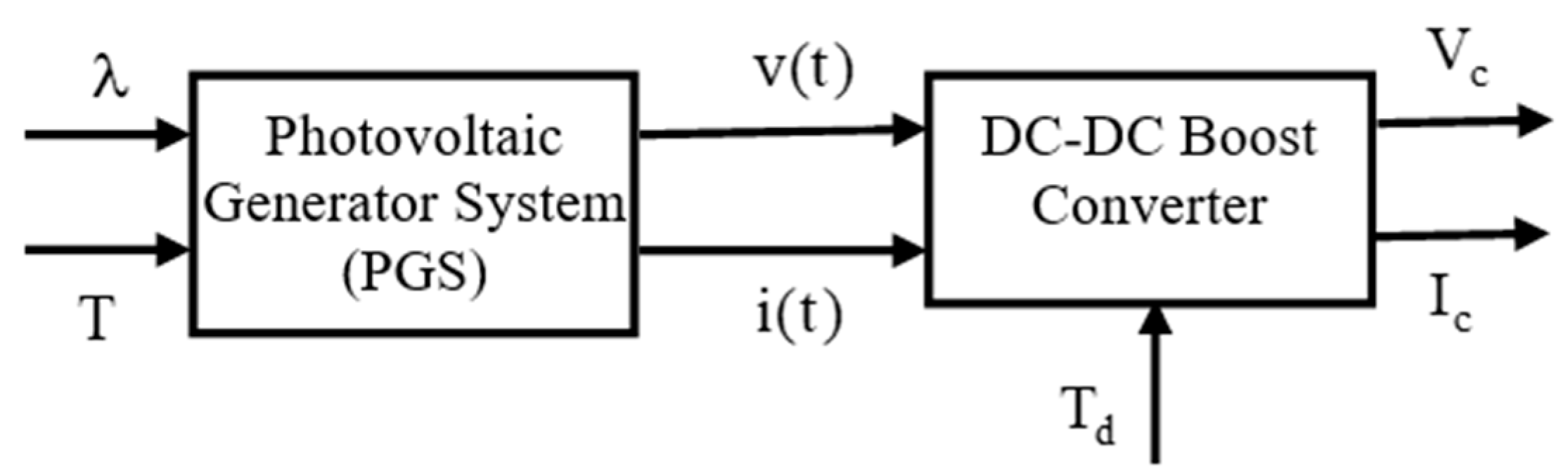
2. Photovoltaic Model Structure
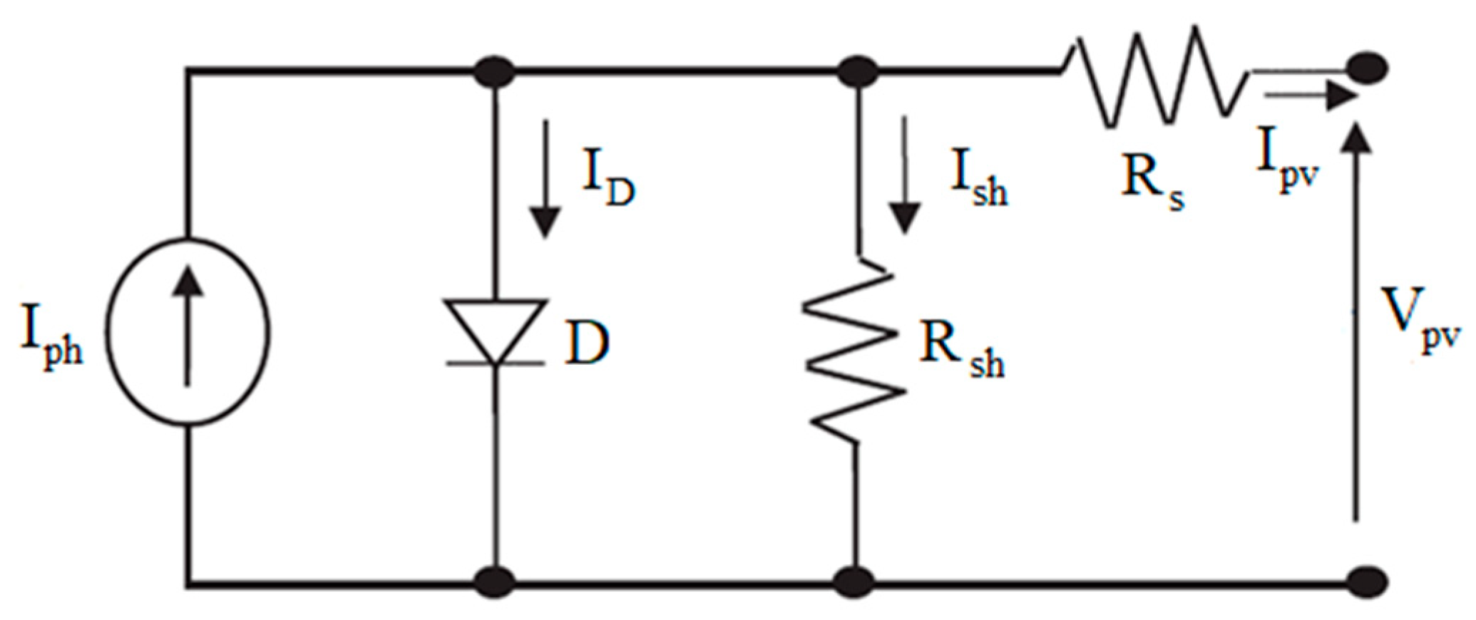
2.1. PVGS Model
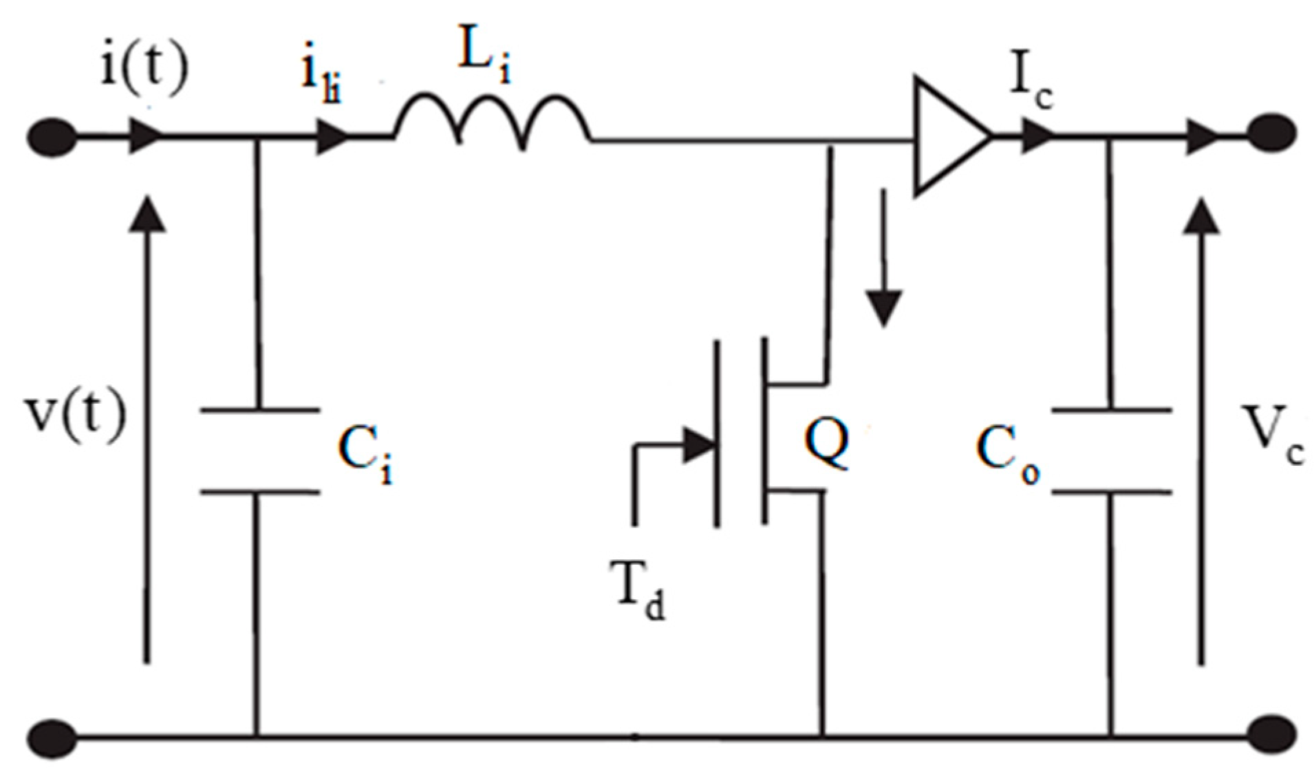
2.2. IBC Model
3. MPPT Structure
4. Observer and Controller Design
4.1. Proposed SMO
4.2. Proposed DSMC
4.3. CSMC Design
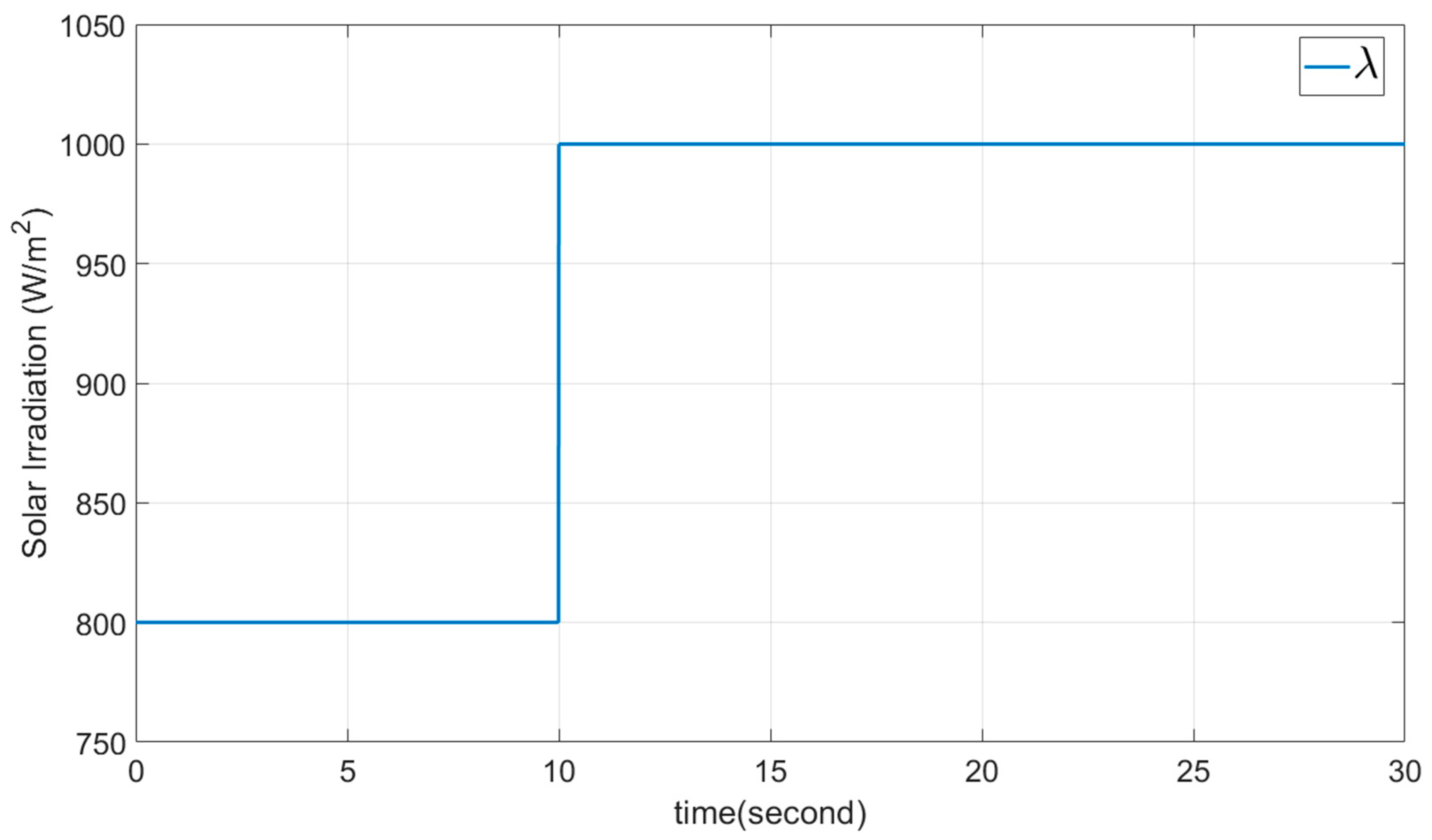
5. Presentation of Simulation Results
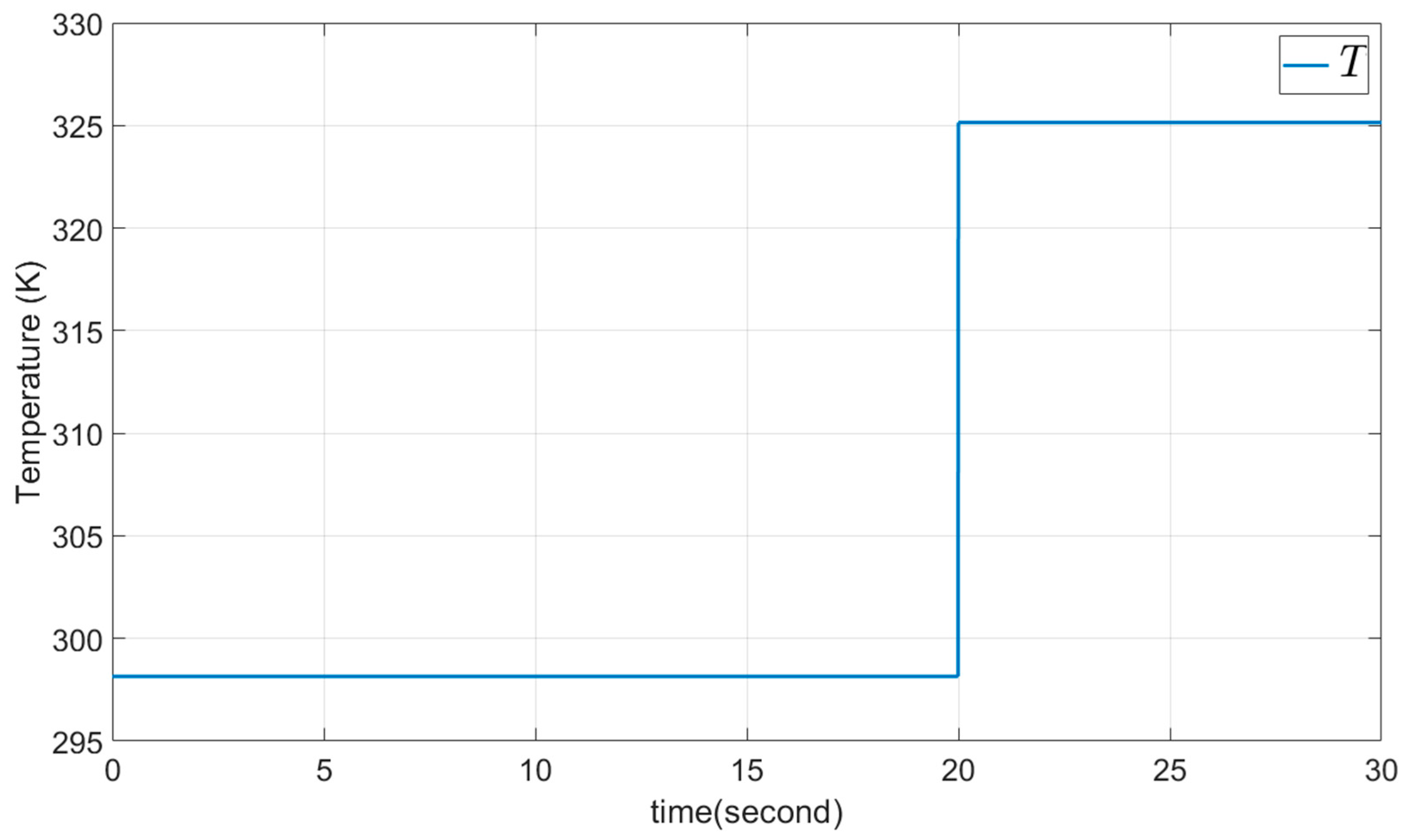
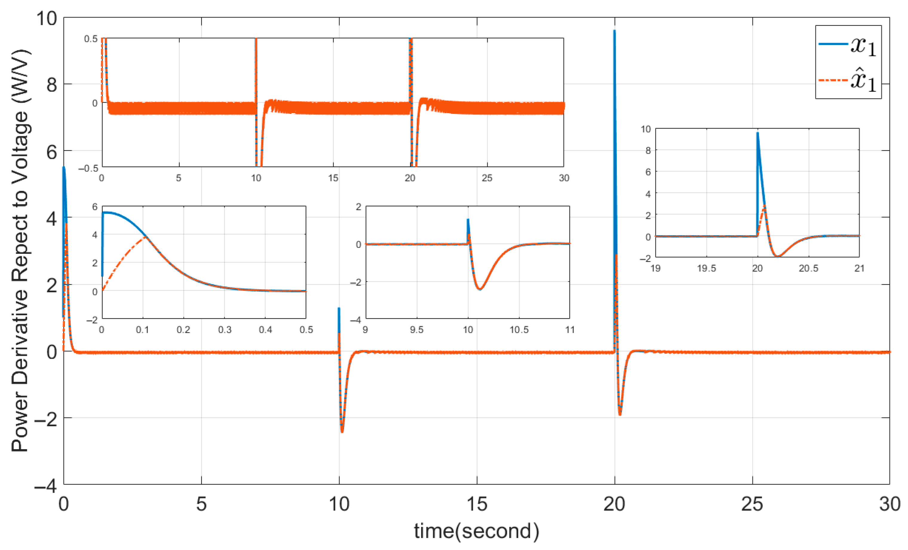
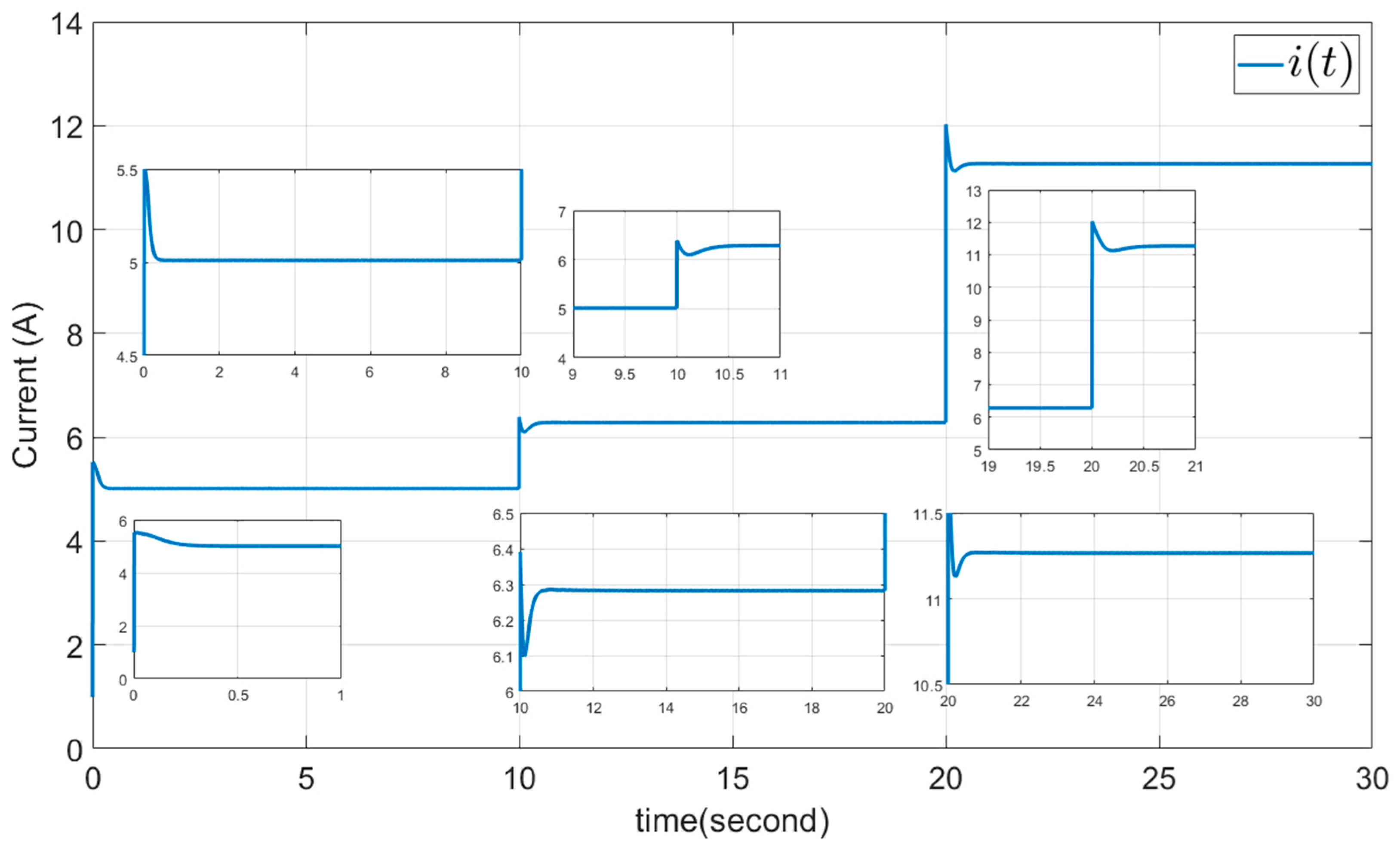
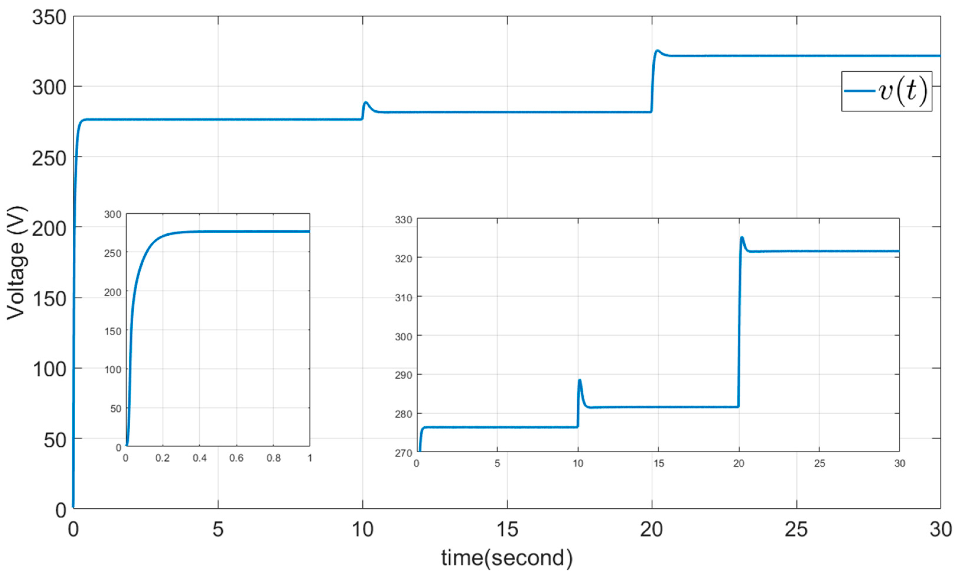
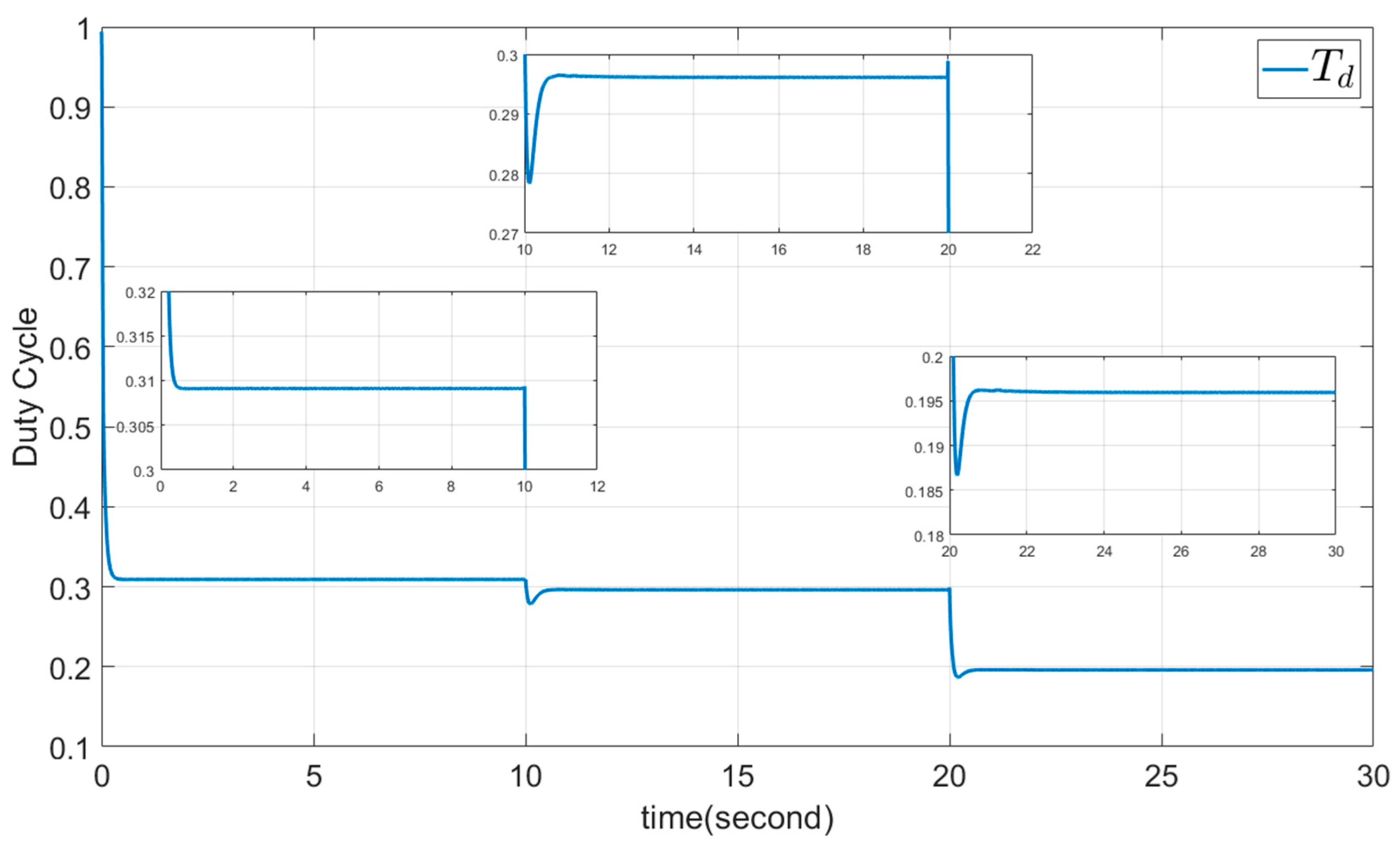
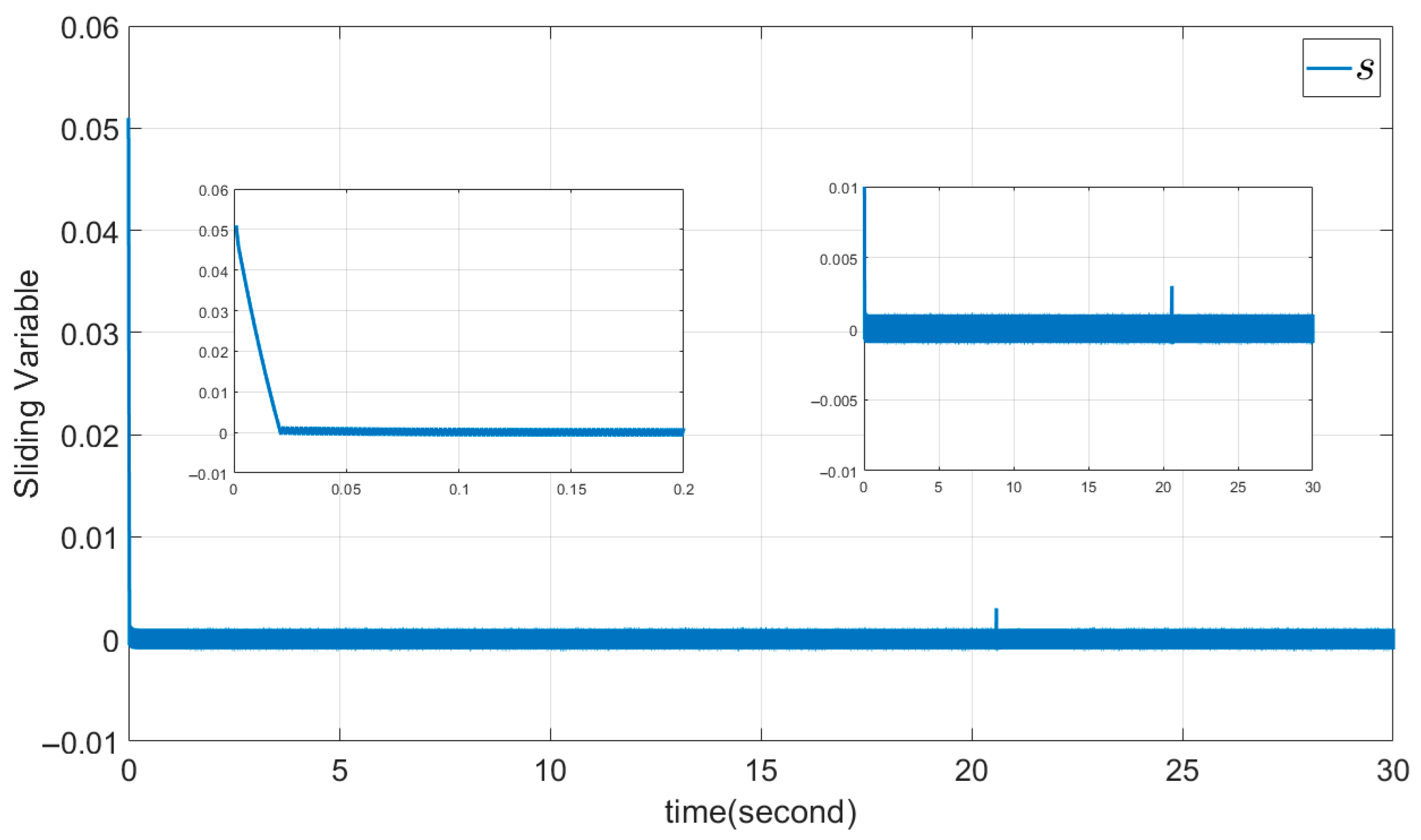
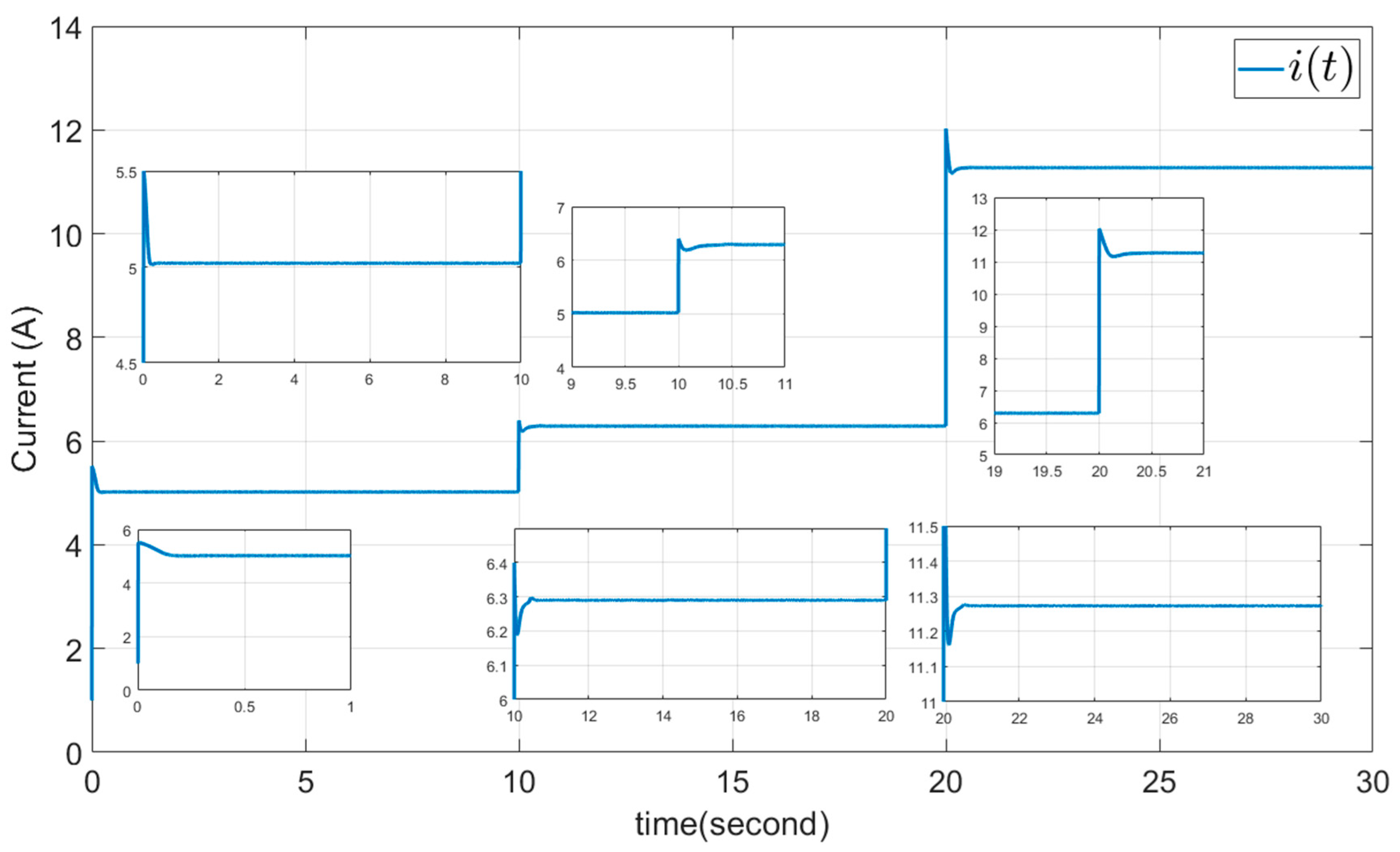
5.1. Example 1: The DSMC Proposed Method
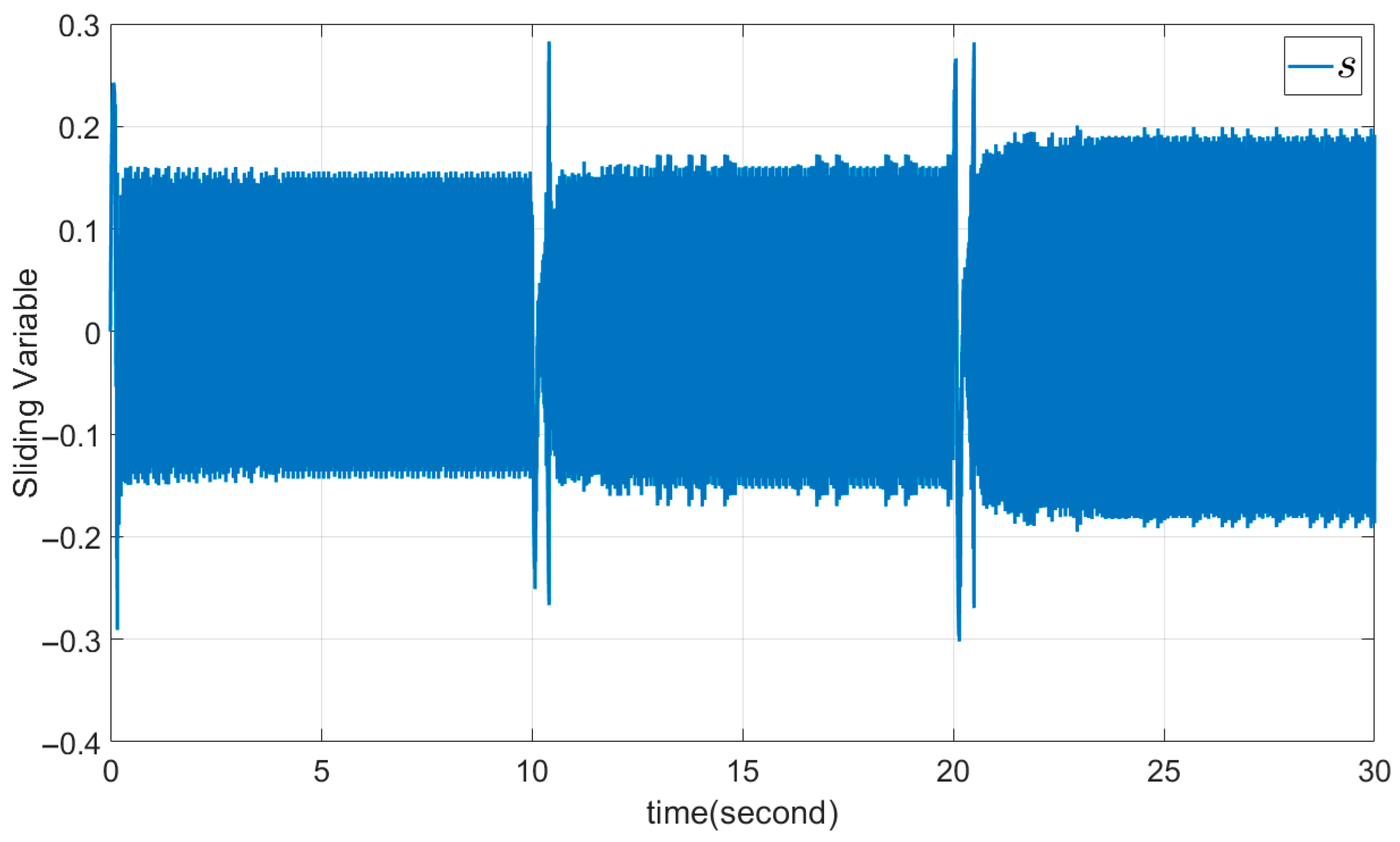
5.2. Example 2: The CSMC Approach
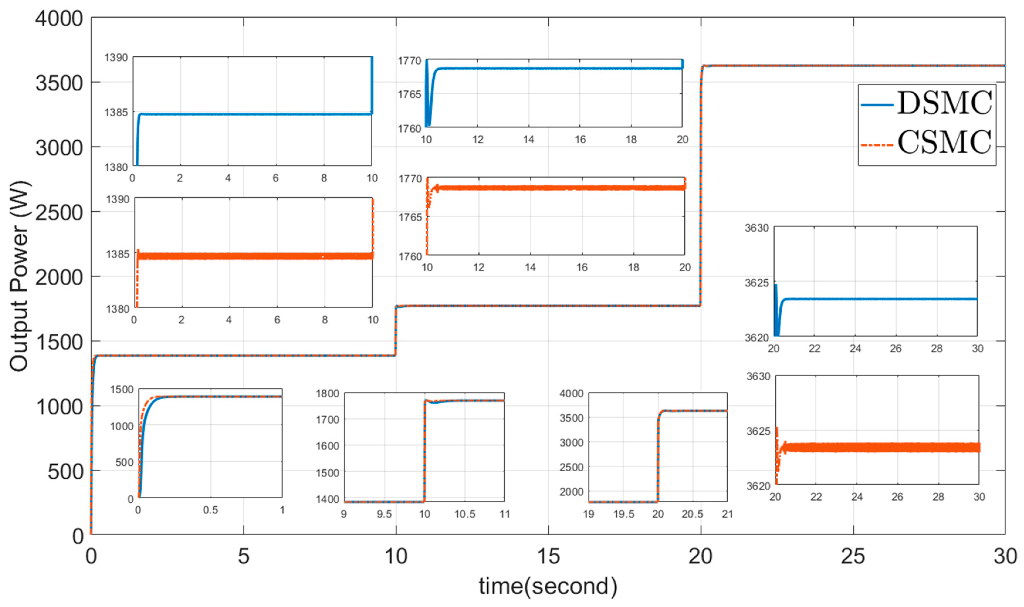
5.3. Comparison Results: The DSMC and CSMC Approach
6. Conclusions
Author Contributions
Funding
Data Availability Statement
Acknowledgments
Conflicts of Interest
References
- Saemian, M.; Bergadà, J.M. Active flow control actuators on wind turbines; comprehensive review. Ocean Eng. 2025, 339, 121991. [Google Scholar] [CrossRef]
- Karami-Mollaee, A.; Barambones, O. On neural observer in dynamic sliding mode control of permanent magnet synchronous wind generator. Mathematics 2024, 12, 2246. [Google Scholar] [CrossRef]
- Wang, W.; Dong, Y.; Liu, Y.; Li, R.; Wang, C. Inductor current-based control strategy for efficient power tracking in distributed PV systems. Mathematics 2024, 12, 3897. [Google Scholar] [CrossRef]
- Karami-Mollaee, A.; Barambones, O. Dynamic sliding mode control of DC-DC converter to extract the maximum power of photovoltaic system using dual sliding observer. Electronics 2022, 11, 2506. [Google Scholar] [CrossRef]
- Karami, N.; Moubayed, N.; Outbib, R. General review and classification of different MPPT techniques. Renew. Sustain. Energy Rev. 2017, 68, 1–18. [Google Scholar] [CrossRef]
- Adhikari, S.; Li, F.; Li, H. P-Q and P-V control of photovoltaic generators in distribution systems. IEEE Trans. Smart Grid 2015, 6, 2929–2941. [Google Scholar] [CrossRef]
- El Khazane, J.; Tissir, E.H. Achievement of MPPT by finite time convergence sliding mode control for photovoltaic pumping system. Sol. Energy 2018, 166, 13–20. [Google Scholar] [CrossRef]
- Belhadj, S.M.; Meliani, B.; Benbouhenni, H.; Zaidi, S.; Elbarbary, Z.M.S.; Alammar, M.M. Control of multi-level quadratic DC-DC boost converter for photovoltaic systems using type-2 fuzzy logic technique-based MPPT approaches. Heliyon 2025, 11, e42181. [Google Scholar] [CrossRef]
- Ahmad, F.F.; Ghenai, C.; Hamid, A.K.; Bettayeb, M. Application of sliding mode control for maximum power point tracking of solar photovoltaic systems: A comprehensive review. Annu. Rev. Contr. 2020, 49, 173–196. [Google Scholar] [CrossRef]
- Elbaksawi, O. Design of photovoltaic system using buck-boost converter based on MPPT with PID controller. Univers. J. Elect. Electron. Eng. 2019, 6, 314–322. [Google Scholar] [CrossRef]
- Aouani, N.; Olalla, C. Robust LQR control for PWM converters with parameter-dependent Lyapunov functions. Appl. Sci. 2020, 10, 7534. [Google Scholar] [CrossRef]
- Ali, A.I.; Sayed, M.A.; Mohamed, E.E. Modified efficient perturb and observe maximum power point tracking technique for grid-tied PV system. Int. J. Elect. Power Energy Sys. 2018, 99, 192–202. [Google Scholar] [CrossRef]
- Girgis, M.E.; Elkhateeb, N.A. Enhancing photovoltaic MPPT with P&O algorithm performance based on adaptive PID control using exponential forgetting recursive least squares method. Renew. Energy 2024, 237, 121801. [Google Scholar] [CrossRef]
- Huang, B.; Song, K.; Jiang, S.; Zhao, Z.; Zhang, Z.; Li, C.; Sun, J. A robust Salp swarm algorithm for photovoltaic maximum power point tracking under partial shading conditions. Mathematics 2024, 12, 3971. [Google Scholar] [CrossRef]
- Dehghanzadeh, A.; Farahani, G.; Vahedi, H.; Al-Haddad, K. Model predictive control design for DC-DC converters applied to a photovoltaic system. Int. J. Elect. Power Energy Sys. 2018, 103, 537–544. [Google Scholar] [CrossRef]
- Dounis, A.I.; Kofinas, P.; Papadakis, G.; Alafodimos, C. A direct adaptive neural control for maximum power point tracking of photovoltaic system. Sol. Energy 2015, 115, 145–165. [Google Scholar] [CrossRef]
- Abbassi, R.; Saidi, S. Design of a novel chaotic Horse Herd Optimizer and application to MPPT for optimal performance of stand-alone solar PV water pumping systems. Mathematics 2024, 12, 594. [Google Scholar] [CrossRef]
- Nabipour, M.; Razaz, M.; Seifossadat, S.; Mortazavi, S. A new MPPT scheme based on a novel fuzzy approach. Renew. Sustain. Energy Rev. 2017, 74, 1147–1169. [Google Scholar] [CrossRef]
- Ramadan, A.; Kamel, S.; Hamdan, I.; Agwa, A.M. A novel intelligent ANFIS for the dynamic model of photovoltaic systems. Mathematics 2022, 10, 1286. [Google Scholar] [CrossRef]
- Miqoi, S.; El Ougli, A.; Tidhaf, B. Adaptive fuzzy sliding mode based MPPT controller for a photovoltaic water pumping system. Int. J. Power Electron. Drive Sys. 2019, 10, 414–422. [Google Scholar] [CrossRef]
- Slotine, J.J.E.; Li, W. Applied Nonlinear Control; Prentice Hall: Englewood Cliffs, NJ, USA, 1991. [Google Scholar]
- Karami-Mollaee, A.; Tirandaz, H. Estimation of load torque in induction motors via dynamic sliding mode control and new nonlinear state observer. J. Mech. Sci. Tech. 2018, 32, 2283–2288. [Google Scholar] [CrossRef]
- Perruquetti, W.; Barbot, J.P. Sliding Mode Control in Engineering; Marcel Dekker: New York, NY, USA, 2002. [Google Scholar]
- Aminnejhad, H.; Kazeminia, S.; Aliasghary, M. Robust sliding-mode control for maximum power point tracking of photovoltaic power systems with quantized input signal. Optik 2021, 247, 167983. [Google Scholar] [CrossRef]
- Yatimi, H.; Aroudam, E. Assessment and control of a photovoltaic energy storage system based on the robust sliding mode MPPT controller. Sol. Energy 2016, 139, 557–568. [Google Scholar] [CrossRef]
- Cortajarena, J.A.; Barambones, O.; Alkorta, P.; De Marcos, J. Sliding mode control of grid-tied single-phase inverter in a photovoltaic MPPT application. Sol. Energy 2017, 155, 793–804. [Google Scholar] [CrossRef]
- Mojallizadeh, M.R.; Badamchizadeh, M.A. Second-order fuzzy sliding-mode control of photovoltaic power generation systems. Sol. Energy 2017, 149, 332–340. [Google Scholar] [CrossRef]
- Kumar, N.; Saha, T.K.; Dey, J. Sliding mode control, implementation and performance analysis of standalone PV fed dual inverter. Sol. Energy 2017, 155, 1178–1187. [Google Scholar] [CrossRef]
- Kchaou, A.; Naamane, A.; Koubaa, Y.; M’sirdi, N. Second order sliding mode-based MPPT control for photovoltaic applications. Sol. Energy 2017, 155, 758–769. [Google Scholar] [CrossRef]
- Chihi, A.; Azza, H.B.; Jemli, M.; Sellami, A. Nonlinear integral sliding mode control design of photovoltaic pumping system: Real time implementation. ISA Trans. 2017, 70, 475–485. [Google Scholar] [CrossRef]
- Lee, H.; Utkin, V.-I. Chattering suppression methods in sliding mode control systems. Annu. Rev. Contr. 2007, 31, 179–188. [Google Scholar] [CrossRef]
- Fuh, C.-C. Variable-thickness boundary layers for sliding mode control. J. Mar. Sci. Tech. 2008, 16, 288–294. [Google Scholar] [CrossRef]
- Chen, H.-M.; Renn, J.-C.; Su, J.-P. Sliding mode control with varying boundary layers for an electro-hydraulic position servo system. Int. J. Adv. Manuf. Tech. 2005, 26, 117–123. [Google Scholar] [CrossRef]
- Zhang, X. Sliding mode-like fuzzy logic control with adaptive boundary layer for multiple-variable discrete. J. Intell. Sys. 2016, 25, 209–220. [Google Scholar] [CrossRef]
- Allamehzadeh, H.; Cheung, J.Y. Optimal fuzzy sliding mode control with adaptive boundary layer. WSEAS Trans. Sys. 2004, 3, 1887–1892. [Google Scholar]
- Cao, T.N.T.; Pham, B.T.; Nguyen, N.T.; Vu, D.-L.; Truong, N.-V. Second-order terminal sliding mode control for trajectory tracking of a differential drive robot. Mathematics 2024, 12, 2657. [Google Scholar] [CrossRef]
- Zhu, Q.; Zhang, J.; Liu, Z.; Yu, S. Robust higher-order nonsingular terminal sliding mode control of unknown nonlinear dynamic systems. Mathematics 2025, 13, 1559. [Google Scholar] [CrossRef]
- Karami-Mollaee, A.; Barambones, O. Higher order sliding mode control of MIMO induction motors: A new adaptive approach. Mathematics 2023, 11, 4558. [Google Scholar] [CrossRef]
- Chen, M.-S.; Chen, C.-H.; Yang, F.-Y. An LTR-observer based dynamic sliding mode control for chattering reduction. Automatica 2007, 43, 1111–1116. [Google Scholar] [CrossRef]
- Karami-Mollaee, A. Design of dynamic sliding mode controller for active suspension system. Modares Mech. Eng. 2016, 16, 51–58. [Google Scholar]
- Karami-Mollaee, A.; Tirandaz, H. Adaptive fuzzy fault tolerant control using dynamic sliding mode. Int. J. Contr. Autom. Sys. 2018, 16, 360–367. [Google Scholar] [CrossRef]
- Wang, H.; Zhang, G.; Liu, X. Sensorless control of surface-mount permanent-magnet synchronous motors based on an adaptive super-twisting sliding mode observer. Mathematics 2024, 12, 2029. [Google Scholar] [CrossRef]
- Raouf, A.H.; Yazdiniya, F.S.; Ansarifar, G.R. Super-twisting ADRC for maximum power point tracking control of photovoltaic power generation system based on non-linear extended state observer. Heliyon 2024, 10, e36428. [Google Scholar] [CrossRef]
- Yang, Y.; Qin, S.; Jiang, P. A modified super-twisting sliding mode control with inner feedback and adaptive gain schedule. Int. J. Adapt. Control Signal Process. 2017, 31, 398–416. [Google Scholar] [CrossRef]
- Rodak, D.; Żurawski, M.; Pyrz, M.; Zalewski, R. Modelling and identification of hysteresis of Vacuum Packed Particles Torsional Damper. J. Sound Vib. 2025, 616, 119203. [Google Scholar] [CrossRef]
- Davila, J.; Fridman, L.; Levant, A. Second-order sliding mode observer for mechanical systems. IEEE Trans. Automat. Contr. 2005, 50, 1785–1789. [Google Scholar] [CrossRef]
- Deng, Q.Q.; Luo, C.U.; Wu, Y.; Li, G.M.; Ling, X.J.; Liang, Z.C. Wind farm parameter optimization identification method based on multi-agent SAC. Energy Rep. 2025, 14, 205–215. [Google Scholar] [CrossRef]
- Li, X.; Zhao, Y. The identification of parameter in a finite set under one-bit quantized observations. Automatica 2025, 180, 112467. [Google Scholar] [CrossRef]
- Fuyang, C.; Lei, W.; Zhang, K.; Tao, G.; Jiang, B. A novel nonlinear resilient control for a quadrotor UAV via backstepping control and nonlinear disturbance observer. Nonlinear Dyn. 2016, 85, 1281–1295. [Google Scholar] [CrossRef]
- Xiong, Y.; Saif, M. Sliding mode observer for nonlinear uncertain systems. IEEE Trans. Automat. Contr. 2001, 46, 2012–2017. [Google Scholar] [CrossRef]
- You, L.; Li, X. Observer-based sliding mode control of impulsive systems with unknown mismatched disturbances. Expert Syst. Appl. 2025, 276, 127092. [Google Scholar] [CrossRef]
- Akbaba, M. Optimum matching parameters of an MPPT unit based for a PVG-powered water pumping system for maximum power transfer. Int. J. Energy Res. 2006, 30, 395409. [Google Scholar] [CrossRef]


| Parameter | Acronym |
|---|---|
| Adaptive Boundary Layer Sliding Mode Control | ABL-SMC |
| Adaptive Neuro-Fuzzy Inference System | ANFIS |
| Boundary Layer Sliding Mode Control | BL-SMC |
| Conventional Sliding Mode Control | CSMC |
| Dynamic Sliding Mode Control | DSMC |
| Higher Order Sliding Mode Control | HOSMC |
| Increasing Boost Converter | IBC |
| Linear Quadratic Regulator | LQR |
| Maximum Power Point Tracking | MPPT |
| Particle Swarm Optimization | PSO |
| Perturb and Observed | P&O |
| Photovoltaic | PV |
| Photovoltaic Generator Systems | PVGS |
| Proportional Integral Derivative | PID |
| Pulse Width Modulation | PWM |
| Root Mean Square | RMS |
| Sliding Mode Control | SMC |
| Sliding Mode Observers | SMO |
| Symmetric Positive Definite | SPD |
| Parameter | Value | Unit |
|---|---|---|
| 4.842 | ||
| 3.45 | ||
| 0.1124 | ||
| 6500 | ||
| 298.15 |
| Parameter | Value | Unit |
|---|---|---|
| 400 | ||
| 12.5 | ||
| 3.5 | ||
| 4700 | ||
| 470 |
| Methods | DSMC | CSMC | ||||
|---|---|---|---|---|---|---|
| Parameter | Min | Max | RMS | Min | Max | RMS |
| −2.4387 | 9.6121 | 0.5074 | −1.4473 | 9.649 | 0.4012 | |
| −2.4537 | 3.8309 | 0.3238 | −1.4577 | 1.81 | 0.1637 | |
| 1 | 12.0259 | 7.9905 | 1 | 12.0286 | 7.9976 | |
| 1.1489 | 325.3517 | 293.5982 | 1.1489 | 324.4607 | 293.3747 | |
| 0.1866 | 0.994 | 0.2737 | 0.1881 | 0.994 | 0.2736 | |
| −0.0011 | 0.051 | 0.0012 | −0.3021 | 0.2829 | 0.0961 | |
Disclaimer/Publisher’s Note: The statements, opinions and data contained in all publications are solely those of the individual author(s) and contributor(s) and not of MDPI and/or the editor(s). MDPI and/or the editor(s) disclaim responsibility for any injury to people or property resulting from any ideas, methods, instructions or products referred to in the content. |
© 2025 by the authors. Licensee MDPI, Basel, Switzerland. This article is an open access article distributed under the terms and conditions of the Creative Commons Attribution (CC BY) license (https://creativecommons.org/licenses/by/4.0/).
Share and Cite
Karami-Mollaee, A.; Barambones, O. Maximum Power Extraction of Photovoltaic Systems Using Dynamic Sliding Mode Control and Sliding Observer. Mathematics 2025, 13, 2305. https://doi.org/10.3390/math13142305
Karami-Mollaee A, Barambones O. Maximum Power Extraction of Photovoltaic Systems Using Dynamic Sliding Mode Control and Sliding Observer. Mathematics. 2025; 13(14):2305. https://doi.org/10.3390/math13142305
Chicago/Turabian StyleKarami-Mollaee, Ali, and Oscar Barambones. 2025. "Maximum Power Extraction of Photovoltaic Systems Using Dynamic Sliding Mode Control and Sliding Observer" Mathematics 13, no. 14: 2305. https://doi.org/10.3390/math13142305
APA StyleKarami-Mollaee, A., & Barambones, O. (2025). Maximum Power Extraction of Photovoltaic Systems Using Dynamic Sliding Mode Control and Sliding Observer. Mathematics, 13(14), 2305. https://doi.org/10.3390/math13142305