The Kinematics of a New Schönflies Motion Generator Parallel Manipulator Using Screw Theory

Abstract

In this work, an innovative Schönflies motion generator manipulator is introduced, featuring a parallel architecture composed of serial chains with mixed degrees of freedom. Fundamental kinematic aspects essential to any manipulator such as displacement, velocity, acceleration, and singularity analyses are thoroughly addressed. Screw theory is employed to derive compact input–output expressions for velocity and acceleration, leveraging the properties of reciprocal screws and lines associated with the constrained degrees of freedom in the parallel manipulator. A key advantage of the proposed design is its near-complete avoidance of singular configurations, which significantly enhances its applicability in robotic manipulation. Numerical examples are provided to validate the theoretical results, with corroboration from specialized tools such as ADAMS™ software and data fitting algorithms. These results confirm the reliability and robustness of the developed kinematic analysis approach.

1. Introduction

Many industrial applications require robotic manipulators with fewer than six degrees of freedom. A Schönflies mechanism is a four-degree-of-freedom system widely used in robotics, capable of generating 3T1R motion. It is named after the German mathematician Arthur Schönflies, who made significant contributions to group theory and the kinematics of mechanisms. This type of mechanism enables three translational and one rotational movement in three-dimensional space—referred to concisely as 3T1R. Over recent decades, Schönflies mechanisms have gained popularity in industrial applications that demand precise and controlled motion, such as object manipulation and part assembly. In this context, 3T1R motion is highly valued for tasks like packaging, picking, and palletizing. A well-known example of a Schönflies mechanism is the seminal Delta robot developed by Clavel [1], which is extensively used on production lines for pick-and-place operations. In a relatively short period, Schönflies mechanisms have achieved a prominent position in both academia and industry. Today, the fastest and most accurate robots are often based on architectures that emulate 3T1R motion with remarkable dexterity. Performance capabilities such as executing up to 240 pick-and-place operations per minute and achieving accelerations of 200 m/s² with payloads of up to two kilograms are feats that are difficult to match with serial manipulators. Given this scenario, interest in the development of Schönflies motion generator parallel manipulators has grown substantially in recent decades. This growing attention has driven a significant number of high-quality contributions addressing, in a consistent and rigorous manner, key aspects such as the kinematics, dynamics, and control of these robotic systems.

Altuzarra et al. [2] reported the development of a four-degree-of-freedom symmetric parallel Schönflies motion generator, inspired by a previous robot design with linear inputs. Their research includes detailed kinematic analyses, such as the use of group theory to confirm the degrees of freedom, the solution of direct and inverse position problems to determine the workspace, and a Jacobian-based analysis. Additionally, they explored isotropic configurations and mapped local dexterity within the workspace, providing valuable insights into the manipulator’s performance. Rico et al. [3] proposed an approach for assessing the dexterity of Schönflies parallel manipulators through angularity and axiality indices, which are useful in evaluating the sensitivity of the moving platform’s motion. Notably, these dexterity indices do not necessarily require a dimensionally homogeneous Jacobian matrix, as is the case with classical methods. Isaksson et al. [4] investigated Schönflies motion in kinematically redundant parallel manipulators composed of two platform sections connected by a passive joint. Their use of screw theory to analyze singularities—particularly redundant passive motion singularities—represents a rigorous and insightful approach. The distinction between full-rank wrench systems on one platform section and rank-deficient systems on the other underscores the delicate balance needed to maintain control and precision. Cao et al. [5] presented a method for analyzing the stiffness of overconstrained parallel robotic mechanisms capable of replicating SCARA motion. Their approach involves deriving the stiffness model of a limb by applying Castigliano’s second theorem to its strain energy, using a structural decomposition strategy. Based on these limb stiffness models and the static equilibrium equation of the moving platform, they established the stiffness matrix of the overall mechanism. Gallardo-Alvarado et al. [6] conducted a study on the kinematics and dynamics of a 4-PRUR parallel manipulator, combining screw theory with the principle of virtual work to understand motion and force transmission. The inclusion of pseudo-revolute joints to ensure full-rank Jacobian matrices is a particularly effective strategy for addressing kinematic constraints. Screw algebra has proven to be a robust and elegant mathematical framework for elucidating the kinematics and dynamics of Schönflies motion generator parallel manipulators [4,7,8,9,10]. Arian et al. [11] investigated the kinematics and dynamics of a parallel manipulator with infinite tool rotation, well-suited for tasks requiring controlled, repetitive motion—such as fabric cutting and electronic assembly, where precision is critical. Wu et al. [12] developed a four-legged parallel manipulator featuring a planetary gear train that enables the full-circle rotation of the end-effector. Their analysis covers workspace, dexterity, and singularity. Avoiding singular configurations by managing working modes and the end-effector’s rotation direction is an effective strategy to ensure smooth operation. Furthermore, the depiction of a super-ellipsoidal workspace emphasizes the manipulator’s adaptability to precise and dexterous tasks. To address the growing demand for high-speed, high-precision applications, Men et al. [13] introduced an articulated-platform parallel robot capable of Schönflies motion. Its design is based on a modified type synthesis method, incorporating principles from Grassmann line geometry and line graph theory. The use of closed-ended revolute/universal joints effectively eliminates errors typically found in closed-loop passive limbs. Urrea et al. [14] presented the virtual design of a four-arm Delta parallel robot for use in the automated preparation of fast food. Kinematic and dynamic models were developed based on the robot’s morphology, followed by the design and implementation of control strategies, specifically Fuzzy PD and Fuzzy PID—previously unexplored for this type of manipulator. A notable contribution is the development of a comprehensive dynamic model in Simscape, which incorporates realistic elements often overlooked in analytical models. To enhance accuracy, external disturbance rejection was rigorously examined through simulations that account for time delays and control signal saturation.

In this work, a four-legged Schönflies motion generator parallel manipulator is introduced, composed of serial kinematic chains with two different degrees of freedom. To explain the topology and kinematics of the proposed robot, the paper is organized as follows. Section 2 presents the architecture of the 3T1R robot, along with the notation used throughout the paper. The mechanism’s mobility is investigated using screw theory. In this context, a standard basis for manipulators that generate 3T1R motion is examined. The constraint systems associated with the limited-degree-of-freedom limbs are analyzed to better understand the mechanism’s constrained motions. This analysis clarifies how the various joints and links interact to produce the overall motion of the robot. Section 3 addresses the displacement analysis based on the closure equations of the parallel manipulator. The direct position analysis is computationally intensive, involving the solution of a system of three quadratic equations, which is mathematically complex and may yield multiple solutions. In contrast, the inverse position analysis is significantly simpler, resulting in a unique, straightforward solution, making it more practical for real-world applications. The instantaneous kinematics of the robot is discussed in Section 4. Input–output equations for velocity and acceleration are derived in compact form using screw theory, effectively capturing the essential kinematic behavior of the robot. This kinematic analysis is complemented by a singularity analysis of the parallel manipulator. To numerically illustrate the kinematic methodology developed in the paper, Section 5 presents several application examples covering most of the topics discussed. Finally, the paper concludes with a summary of findings and final remarks.

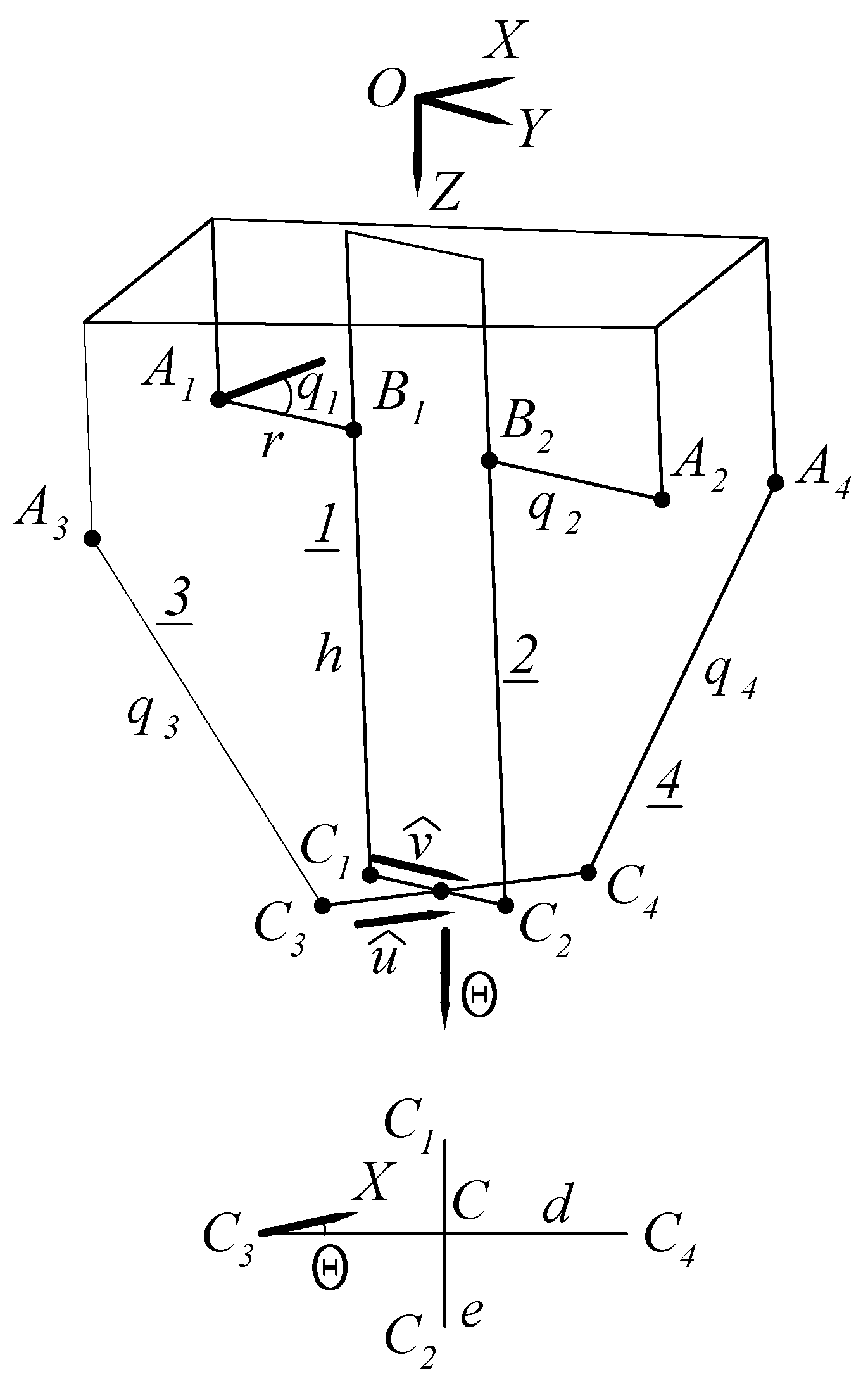
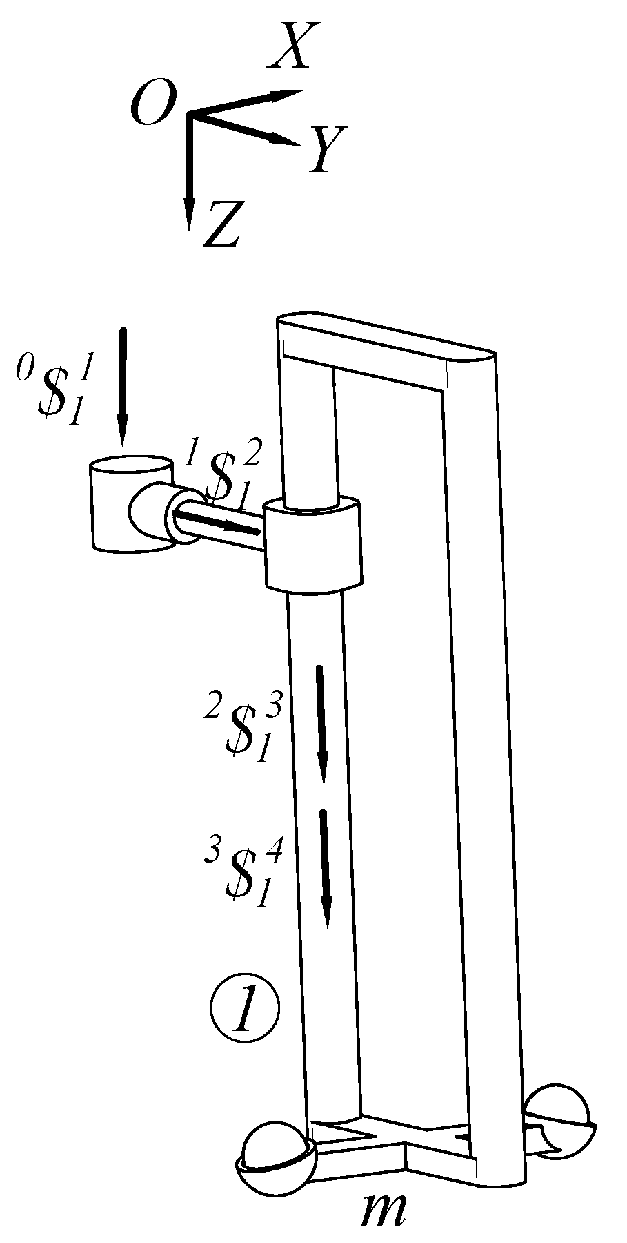
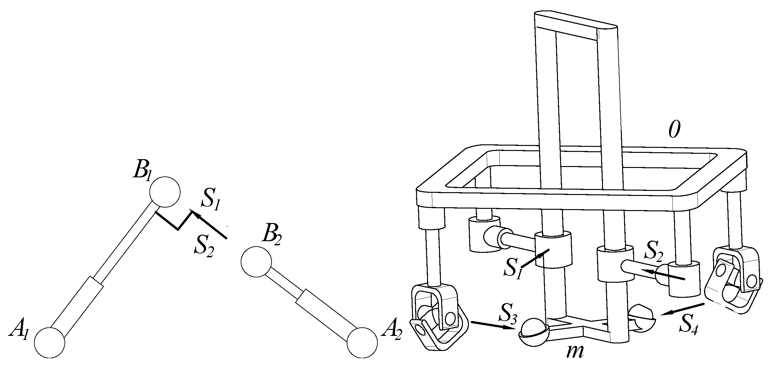
2. Description of the Robot Manipulator

With reference to Figure 1, the proposed parallel manipulator comprises a three-dimensional moving platform m linked to the fixed platform 0 using four limbs, two of the RPC-type, labeled 1 and 2, and two of the UPS-type, labeled 3 and 4. The acronym “RPC” stands for Revolute-Prismatic-Cylindrical while the acronym “UPS” stands for Universal-Prismatic-Spherical. These describe the type of joints in the limbs. Furthermore, the moving platform m consists of two rigidly joined solids: one rectangular and the other cross-shaped, forming a three-dimensional structure. This kind of platform presents notable advantages over its planar counterpart, including enhanced workspace, improved manipulability, and simplified kinematic analysis [15].

In what follows, the elementary notation of the parallel manipulator is introduced. To this end, let us consider that $O\_XYZ$ is a reference frame attached to the fixed platform with the Z-axis normal to the plane of the fixed platform; see Figure 2. The centers of the U-joints are notated by points $A_3$ and $A_4$ while $C_3$ and $C_4$ denote the centers of the S-joints. Meanwhile, the nominal position of the R-joints are designated by points $A_1$ and $A_2$. Furthermore, the nominal position of the C-joints are notated by points $B_1$ and $B_2$. Each point P is located by its position vector $\mathit{p}$. On the other hand, h denotes the offset between points $B_i$ and $C_i$ in the same i-th limb, whereas r is the distance between points $A_1$ and $B_1$ or extendible length of the unique passive P-joint. To specify the orientation of the moving platform, let us consider two unit vectors $\widehat{\mathit{u}}$ and $\widehat{\mathit{v}}$ where $\widehat{\mathit{u}}$ is directed from $C_3$ to $C_4$ and $\widehat{\mathit{v}}$ is pointed from $C_1$ to $C_2$. The angle $\theta$, measured from the X-axis, is also a way to specify the orientation of the moving platform. Finally, the parameter d denotes the distance between points $C_3$ and $C_4$ while the parameter e denotes the distance between points $C_1$ and $C_2$.

Mobility Analysis

The mobility analysis of parallel manipulators focuses on understanding their degrees of freedom and motion properties. This analysis is crucial for designing and optimizing these systems for specific applications. Key aspects of the mobility analysis comprise determining the number of independent movements that the moving platform can perform, identifying the causes that limit motion such as screw-type constraints, and exploring underactuated, overactuated, and fully actuated mechanisms to optimize control and performance. Dealing with the parallel manipulator under study, it is clear that the limited mobility of the manipulator is due to the inclusion of the RPC-type kinematic chains. This condition of the manipulator can be demonstrated by resorting to the screw theory. To this end, the screw system of the RPC-type kinematic chain is depicted in Figure 3.

To explain the mobility of the parallel manipulator, let us consider that $O\_XYZ$ is a reference frame attached to the fixed platform with associated unit vectors $\widehat{\mathit{i}}\widehat{\mathit{j}}\widehat{\mathit{k}}$ with the Z-axis pointing vertically. The standard or natural basis for parallel manipulators able to replicate the 3T1R motion is given by the system $S=\{{\$}_1,{\$}_2,{\$}_3,{\$}_4\}$ where

$$\begin{array}{c}\hfill {\$}_1=\left[\begin{array}{c}\widehat{\mathit{k}}\\ \mathbf{0}\end{array}\right],{\$}_2=\left[\begin{array}{c}\mathbf{0}\\ \widehat{\mathit{i}}\end{array}\right],{\$}_3=\left[\begin{array}{c}\mathbf{0}\\ \widehat{\mathit{j}}\end{array}\right],{\$}_4=\left[\begin{array}{c}\mathbf{0}\\ \widehat{\mathit{k}}\end{array}\right]\end{array}$$

On the other hand, the elements of the motion-screw system of the RPC-type limb labeled 1 are given by

$$\begin{array}{c}\hfill {}^0\$_1^1=\left[\begin{array}{c}\widehat{\mathit{k}}\\ \widehat{\mathit{k}}\times {\mathit{r}}_{O/A_1}\end{array}\right],{}^1\$_1^2=\left[\begin{array}{c}\widehat{\mathbf{0}}\\ {\widehat{\mathit{r}}}_{B_1/A_1}\end{array}\right],{}^2\$_1^3=\left[\begin{array}{c}\widehat{\mathit{k}}\\ \widehat{\mathit{k}}\times {\mathit{r}}_{O/B_1}\end{array}\right],{}^3\$_1^4=\left[\begin{array}{c}\widehat{\mathbf{0}}\\ \widehat{\mathit{k}}\end{array}\right]\end{array}$$

where ${}^0\$_1^1$ is the screw associated with the revolute joint R while ${}^1\$_1^2$ is the screw associated with the prismatic joint P. Furthermore, the screws ${}^2\$_1^3$ and ${}^3\$_1^4$ simulate the cylindrical joint C, rotation plus translation, respectively. Clearly, we have a two constraint system reciprocal to the aforementioned screws given by

$$\begin{array}{c}\hfill {\$}_i=\left[\begin{array}{c}\widehat{\mathbf{0}}\\ \widehat{\mathit{i}}\end{array}\right],\mathrm{and}{\$}_j=\left[\begin{array}{c}\widehat{\mathbf{0}}\\ \widehat{\mathit{j}}\end{array}\right]\end{array}$$

Therein, ${\$}_i$ is a constraint couple in the X-axis while ${\$}_j$ is a constraint couple in the Y-axis. In other words, the moving platform cannot rotate along the X and Y axes. To reinforce this conclusion, let us consider one variant of the Chebyshev–Grübler–Kutzbach criterion [16,17]. The mobility M of the parallel manipulator may be computed as follows

$$\begin{array}{c}\hfill M=(6-\lambda )(n-g-1)+\sum _{i=1}^g{f}_i+\nu \end{array}$$

(1)

where $\lambda =0$ is the number of independent constraints, $n=10$ is the number of links including the ground, $g=12$ is the number of kinematic pairs, and $f_i$ denotes the freedoms of the i-th link. Thus, ${\sum }_{i=1}^g{f}_i=20$. Furthermore, $\nu =2$ is the number of redundant constraint screws. Gathering these results, one obtains that $M=4$, confirming the limited mobility of the parallel manipulator. Thus, we have the possibility to choose four kinematic pairs as actuated kinematic joints. A natural option is to assign one generalized coordinate $q_i(i\sim 4)$ to each limb. In the work, the selection of actuated joints is specified by the abbreviated notation RPC + RPC + 2UPS of the parallel manipulator, where underlined letters denote actuated joints. Dealing with the RPC-type limbs, the revolute joint R is driven by the rotary actuator $q_1$ while the prismatic joint P is driven by the linear actuator $q_2$. To complete the generalized coordinates $q_i(i\sim 4)$, the prismatic joints of the UPS-type limbs are driven by the linear actuators $q_3$ and $q_4$.

3. Displacement Analysis

The complexity of the kinematic analysis of a manipulator is directly related with its degrees of freedom. When certain degrees of freedom are constrained, the mathematical models and equations needed for position analysis become less intricate, allowing for a more straightforward examination. This is because fewer degrees of freedom mean fewer variables and constraints to account for, significantly reducing computational demands. For the parallel manipulator under study, the fact that there are two constrained degrees of freedom simplifies the displacement analysis considerably.

3.1. Closure Equations

In the kinematic analysis of robot manipulators, the closure equations are mathematical expressions that ensure that their geometric and motion constraints are satisfied. These equations enforce the conditions required for the kinematic joints, links, and the moving platform to maintain their defined relationships during motion. The precision with which closure equations are formulated is essential for their accurate application in the kinematic analysis of parallel manipulators. When these equations are clearly and obviously correctly established, they faithfully represent the geometric and motion constraints of the system, ensuring reliable analysis and results.

The unit vectors $\widehat{\mathit{u}}$ and $\widehat{\mathit{v}}$ attached to the moving platform are defined, according to the fixed reference frame $O\_XYZ$, based on the orientating angle $\theta$ as follows

$$\begin{array}{c}\hfill \widehat{\mathit{u}}=cos\theta \widehat{\mathit{i}}+sin\theta \widehat{\mathit{j}},\widehat{\mathit{v}}=-sin\theta \widehat{\mathit{i}}+cos\theta \widehat{\mathit{j}}\end{array}$$

(2)

where evidently $\widehat{\mathit{u}}·\widehat{\mathit{v}}=0$. To simplify the handling of trigonometric functions, for example, to avoid the use of the identity ${sin}^2\theta +{cos}^2\theta =1$, the trigonometric functions $cos\theta$ and $sin\theta$ may be written introducing the tangent half-angle $\zeta$—see [18]—as follows

$$\begin{array}{c}\hfill cos\theta ={\displaystyle \frac{1-{\zeta }^2}{1+{\zeta }^2}},sin\theta ={\displaystyle \frac{2\zeta }{1+{\zeta }^2}}\end{array}$$

(3)

where

$$\begin{array}{c}\hfill \zeta =tan\theta /2\end{array}$$

(4)

Considering the position vector $\mathit{c}$ of the center C of the moving platform, the position vectors ${\mathit{c}}_i(i=1\sim 4)$ denoting the vertices of the moving platform may be expressed as

$$\begin{array}{c}\hfill {\mathit{c}}_1=\mathit{c}-e\widehat{\mathit{v}}/2,{\mathit{c}}_2=\mathit{c}+e\widehat{\mathit{v}}/2,{\mathit{c}}_3=\mathit{c}-d\widehat{\mathit{u}}/2,{\mathit{c}}_4=\mathit{c}+d\widehat{\mathit{u}}/2\end{array}$$

(5)

Naturally, a position vector may be stated in different ways. For example, the position vectors of the centers of the S-joints can be written involving the generalized coordinate $q_1$ as follows

$$\begin{array}{c}\hfill {\mathit{c}}_3={\mathit{a}}_1+rcos{q}_1\widehat{\mathit{i}}+rsin{q}_1\widehat{\mathit{j}}+h\widehat{\mathit{k}}+(e\widehat{\mathit{v}}-d\widehat{\mathit{u}})/2\end{array}$$

(6)

and

$$\begin{array}{c}\hfill {\mathit{c}}_4={\mathit{a}}_1+rcos{q}_1\widehat{\mathit{i}}+rsin{q}_1\widehat{\mathit{j}}+h\widehat{\mathit{k}}+(e\widehat{\mathit{v}}+d\widehat{\mathit{u}})/2\end{array}$$

(7)

In this sense, the center C of the moving platform is determined, considering that its position vector $\mathit{c}$ may be obtained as

$$\begin{array}{c}\hfill \mathit{c}=({\mathit{c}}_3+{\mathit{c}}_4)/2\end{array}$$

(8)

To complete the coordinates of the kinematic pairs, the point $B_1$ and $B_2$ may be found, considering that their position vectors ${\mathit{b}}_1$ and ${\mathit{b}}_2$ are given by

$$\begin{array}{c}\hfill {\mathit{b}}_1={\mathit{a}}_1+rcos{q}_1\widehat{\mathit{i}}+rsin{q}_1\widehat{\mathit{j}}\end{array}$$

(9)

and

$$\begin{array}{c}\hfill {\mathit{b}}_2={\mathit{a}}_1+rcos{q}_1\widehat{\mathit{i}}+rsin{q}_1\widehat{\mathit{j}}+e\widehat{\mathit{v}}\end{array}$$

(10)

Alternatively, the vectors ${\mathit{b}}_1$ and ${\mathit{b}}_2$ can be expressed as

$$\begin{array}{c}\hfill {\mathit{b}}_1={\mathit{c}}_1-h\widehat{\mathit{k}}\end{array}$$

(11)

and

$$\begin{array}{c}\hfill {\mathit{b}}_2={\mathit{c}}_2-h\widehat{\mathit{k}}\end{array}$$

(12)

Afterwards, based on the generalized coordinates associated with the actuated prismatic joints three closure equations may be written as follows

$$\begin{array}{c}\hfill f_1=({\mathit{b}}_2-{\mathit{a}}_2)·({\mathit{b}}_2-{\mathit{a}}_2)-q_2^2\end{array}$$

(13a)

$$\begin{array}{c}\hfill f_2=({\mathit{c}}_3-{\mathit{a}}_3)·({\mathit{c}}_3-{\mathit{a}}_3)-q_3^2\end{array}$$

(13b)

$$\begin{array}{c}\hfill f_3=({\mathit{c}}_4-{\mathit{a}}_4)·({\mathit{c}}_4-{\mathit{a}}_4)-q_4^2\end{array}$$

(13c)

With Equations (6)–(13), we dispose of the sufficient resources to approach the forward and the inverse position analyses. Considering this, the generalized coordinates $q_i(i\sim 4)$ are the fundamental elements of the forward displacement analysis while the variables r, h, and $\theta$ are the motivation of the inverse position analysis.

3.2. Forward Displacement Analysis

The forward position analysis, usually a challenger task for most parallel manipulators, is concerned with the determination of the pose, position, and orientation of the moving platform, as measured from the fixed platform from its generalized coordinates $q_i(i=1\sim 4)$. That is to say, the coordinates of the center C of the moving platform need to be computed, as does the orientating angle $\theta$. The difficulty of the position analysis arises due to the complex, non-linear equations involved, stemming from the closed-loop structure of such mechanisms. To achieve the forward displacement analysis, the calculation of the variables r, h, and $\zeta$ plays a central role.

The algorithm to perform the forward displacement analysis of the parallel manipulator is summarized in the following steps:

• Define a known set of generalized coordinates $q_i(i=1\sim 4)$.
• Express $cos\theta$ and $sin\theta$ in terms of the tangent half-angle $\zeta$; see Equation (3).
• Define $\widehat{\mathit{u}}$ and $\widehat{\mathit{v}}$ according to Equation (2).
• Compute the position vectors ${\mathit{c}}_3$, ${\mathit{c}}_4$, and ${\mathit{b}}_2$ using Equations (6), (7) and (10), respectively
• From Equation (13), formulate three quadratic equations in the unknowns r, h, and $\zeta$ as follows

  $$\begin{array}{c}\hfill g_i=f_i(1+{\zeta }^2)i=1,2,3\end{array}$$

  (14)
• Solve the three quadratic equations by applying the Sylvester dialytic method of elimination; for details, see [19].
• Compute the vectors ${\mathit{c}}_3$ and ${\mathit{c}}_4$; see Equations (6) and (7).
• Determine the center C of the moving platform based on Equation (8).
• Determine the angle $\theta$, see Equation (4), as

  $$\begin{array}{c}\hfill \theta =arctan\left(2\zeta \right)\end{array}$$

  (15)

After calculating the angle $\theta$ and the coordinates of point C, the pose of the moving platform is then determined. With this algorithm, it is possible to find a maximum of eight solutions, complex and real, of the forward position analysis. Obviously, only real solutions are useful. Certainly, in the context of kinematic analysis, real solutions are essential because they represent physically feasible configurations of the parallel manipulator. Meanwhile, in terms of complex or imaginary solutions, these typically have no practical relevance for the pose or motion of a robot manipulator.

3.3. Inverse Displacement Analysis

The inverse position analysis is stated as the computation of the generalized coordinates $q_i(i=1\sim 4)$, satisfying a specific posture of the moving platform as observed from the fixed platform. In other words, the generalized coordinates must be computed, given the center C of the moving platform and the relative orientation angle $\theta$. The inverse position analysis is typically simpler than the forward position analysis for most parallel manipulators. This is because there is usually a one-to-one mapping between the specified posture of the parallel manipulator and the generalized coordinates, making the equations solvable in a more direct manner. Based on the closure equations of the complex mechanism, the algorithm of the inverse position analysis comprises the following steps:

• Define the pose of the moving platform providing the vector $\mathit{c}$ and the angle $\theta$.
• Compute the unit vectors $\widehat{\mathit{u}}$ and $\widehat{\mathit{v}}$; see Equation (2).
• Compute the vertices ${\mathit{c}}_i(i=1\sim 4)$ of the moving platform; see Equation (5).
• Compute the generalized coordinates $q_3$ and $q_4$ by resorting to Equation (13). Indeed

  $$\begin{array}{c}\hfill q_3={[({\mathit{c}}_3-{\mathit{a}}_3)·({\mathit{c}}_3-{\mathit{a}}_3)]}^{1/2}\end{array}$$

  (16)

  $$\begin{array}{c}\hfill q_4={[({\mathit{c}}_4-{\mathit{a}}_4)·({\mathit{c}}_4-{\mathit{a}}_4)]}^{1/2}\end{array}$$

  (17)
• Determine h as follows

  $$\begin{array}{c}\hfill h=({\mathit{c}}_1-{\mathit{a}}_1)·\widehat{\mathit{k}}\end{array}$$

  (18)
• Compute the position vector ${\mathit{b}}_1$ by applying Equation (11).
• Calculate the generalized coordinate $q_1$ considering that from Equation (9) it follows that

  $$\begin{array}{c}\hfill tan{q}_1={\displaystyle \frac{({\mathit{b}}_1-{\mathit{a}}_1)·\widehat{\mathit{j}}}{({\mathit{b}}_1-{\mathit{a}}_1)·\widehat{\mathit{i}}}}\end{array}$$

  (19)
• Compute the position vector ${\mathit{b}}_2$ by applying Equation (12).
• Compute the generalized coordinate $q_2$ taking into account that from Equation (13a) it follows that

  $$\begin{array}{c}\hfill q_2={[({\mathit{b}}_2-{\mathit{a}}_2)·({\mathit{b}}_2-{\mathit{a}}_2)]}^{1/2}\end{array}$$

  (20)

Therefore, with this algorithm, there is only one solution for the inverse displacement analysis.

4. Instantaneous Kinematics

The instantaneous kinematics of parallel manipulators deals with analyzing their velocity and acceleration at any given instant. This analysis is essential for understanding how the mechanism moves in response to actuator inputs and for designing precise control systems. The mathematical resource to approach the instantaneous kinematics of the parallel manipulator is the theory of screws [20]. Screw theory provides a compact and elegant way to represent rigid body motions, combining linear and angular velocities into a single entity called twist about screw or velocity state. Dealing with the acceleration analysis, linear and angular accelerations are merged into a single entity called the acceleration state. The velocity and acceleration states satisfy the conditions of helical vectorial fields. To formulate the velocity and acceleration analyses of the parallel manipulator, the screws associated with the kinematic joints are depicted in Figure 4.

To simplify the kinematic analysis, it must taken into account that while the UPS-type limb is able to perform general motions of rigid body, the same is not the same with the RPC-type limb since the latter is limited to executing three-dimensional displacements of the rigid body while maintaining a constant orientation of it. That is to say, the revolute, prismatic, and cylindrical joints collaborate to achieve spatial positioning, but they do not allow the moving platform to change its angular orientation. This limitation leads to tedious algebraic operations when performing the kinematic analysis. To remedy this deficiency, a hypothetical universal kinematic joint $\overline{U}$ is added to the RPC kinematic chain and thus the mobility of the limited-dof limb is fictitiously increased considering that we have a RPC$\overline{U}$-type limb. With this in mind, the screws associated with the kinematic pairs of the parallel manipulator are defined as follows. Dealing with the UPS-type limb, the screws ${}^0\$^1$ and ${}^2\$^1$ are associated with the U-joint representing two rotational degrees of freedom around two perpendicular axes. These screws form a plane in the screw system, enabling rotational motion but restricting translations. The screw ${}^2\$^3$ for the P-joint describes linear motion along one axis. It is characterized by a screw with infinite pitch, representing pure translation along the axis of the prismatic joint. The screws ${}^3\$^4$, ${}^4\$^5$, and ${}^5\$^6$, are associated with the S-joint and encompass three rotational degrees of freedom around the three intersecting axes. The S-joint provides a full range of rotations while disallowing any translations. Similarly, for the RPC$\overline{U}$, ${}^0\$^1$ is the screw associated with the R-joint, which allows rotation around a fixed axis. The screw ${}^0\$^1$ has a specific direction corresponding to the rotational axis, and its pitch vanishes because it represents pure rotation. The screw ${}^1\$^2$ is associated with the P-joint. The screws ${}^2\$^3$ and ${}^3\$^4$ are associated with the C-joint. The cylindrical joint combines the motions of a revolute and a prismatic joint along a shared axis. Finally, the screws ${}^4\$^5$ and ${}^5\$^6$ are associated with the hypothetical $\overline{U}$-joint. Regarding this, the joint rates of the fictitious $\overline{U}$-joint vanish.

4.1. Velocity

The instantaneous kinematics at the level of velocity of the moving platform m can be characterized if one knows the two vectors measured from the fixed platform 0: (i) the angular velocity vector of the moving platform, denoted as ${}^0\mathit{\omega }^m$, and (ii) the velocity vector of a point P on the moving platform, notated as ${}^0\mathit{v}_P^m$, where point P is called the reference pole. The vectors ${}^0\mathit{\omega }^m$ and ${}^0\mathit{v}_P^m$ can be merged into one entity called the twist about a screw or velocity state, which is denoted as ${}^0\mathit{V}_P^m$. More specifically, the velocity state ${}^0\mathit{V}_P^m$ is neatly defined as

$$\begin{array}{c}\hfill {}^0\mathit{V}_P^m=\left[\begin{array}{c}{}^0\mathit{\omega }^m\\ {}^0\mathit{v}_P^m\end{array}\right]\end{array}$$

(21)

where ${}^0\mathit{\omega }^m$ is named the primal part of ${}^0\mathit{V}_P^m$ while ${}^0\mathit{v}_P^m$ is named the dual part of ${}^0\mathit{V}_P^m$. The primal part encapsulates the rotational effect of the motion of the moving body platform whereas the dual part captures the translational aspect of the motion of the moving platform. Hence, the velocity state ${}^0\mathit{V}_P^m$ encapsulates both translational and rotational velocities of the moving platform and is indeed fundamental to describing its motion comprehensively. Representing it as a six-dimensional vector makes it highly versatile in tasks like velocity analysis, motion planning, and control. The velocity state is a unified representation that aligns well with screw theory, which provides a powerful mathematical framework for analyzing and understanding the motion of rigid bodies. In robotics, the velocity state has been a widely used concept thanks to the relationship that can be obtained with a screw in the following way

$$\begin{array}{c}\hfill {}^0\mathit{V}_P^m={}_0\omega _m{}^0\$^m\end{array}$$

(22)

where ${}_0\omega _m=\mid {}^0\mathit{\omega }^m\mid$ is the intensity of the screw ${}^0\$^m$. Thanks to this representation, the velocity state satisfies the conditions of helical vectorial fields [21].

The velocity analysis involves obtaining the relationship between the generalized velocities ${\dot{q}}_i(i=1\sim 4)$ and the velocity state ${}^0\mathit{V}_P^m$ of the moving platform. This relationship is referred to as the input–output equation of velocity and is useful for solving both the forward and the inverse velocity analyses. The screw representation of the velocity state is a highlight of screw theory, offering a compact and efficient way to describe the motion of robotic manipulator links. By combining linear and angular velocity components into a single entity, it provides a framework for analyzing motion along specific axes or screws. Considering this, the velocity state ${}^0\mathit{V}_P^m$ may be written in its screw form through any of the four limbs of the parallel manipulator. With this in mind, by resorting to the UPS-type limbs, the velocity state ${}^0\mathit{V}_C^m$ may be written in screw form as follows

$$\begin{array}{c}\hfill {}_0\omega _1^i{}^0\$_i^1+\dots +{}_4\omega _5^i{}^4\$_i^5+{}_5\omega _6^i{}^5\$_i^6={}^0\mathit{V}_C^{m}i=3,4\end{array}$$

(23)

where the center C of the moving platform is chosen as the reference pole P. Furthermore, ${}_2\omega _3^i={\dot{q}}_i(i=3,4)$ are two active generalized speeds. By utilizing reciprocal lines, passive joint velocities can effectively be “canceled out” from the analysis. This allows the focus to remain solely on the contributions of the active joints to the motion, greatly simplifying the velocity analysis. The concept hinges on the reciprocal relationship between the screws of the passive joints and the wrench system associated with the manipulator. Essentially, passive joints do not contribute to the external wrench imposed on the moving platform, and this property can be exploited mathematically to eliminate their influence. This streamlines the computation of the velocity state and greatly enhances the kinematic analysis of the parallel manipulator. It is clear that the lines along extremities 3 and 4, denoted as $S_3$ and $S_4$, possess the properties described in this paragraph and therefore are categorized as reciprocal lines. Therefore, applying the Klein form, $\left\{\ast ;\ast \right\}$, to both sides of Equation (23), we have a reduction of these equations as follows

$$\begin{array}{c}\hfill {\dot{q}}_i{}^2\$_i^3=\left\{S_i;{}^0\mathit{V}_C^m\right\}i=3,4\end{array}$$

(24)

Following this fashion, from limb 1, it follows that the velocity state ${}^0\mathit{V}_C^m$ may be written in screw form as follows

$$\begin{array}{c}\hfill {}_0\omega _1^1{}^0\$_1^1+\dots +{}_4\omega _5^1{}^4\$_1^5+{}_5\omega _6^1{}^5\$_1^6={}^0\mathit{V}_C^m\end{array}$$

(25)

where ${}_0\omega _1^1={\dot{q}}_1$ is the generalized speed of limb 1 while taking into account that the joint rates ${}_4\omega _5^1$ and ${}_5\omega _6^1$ are associated with a hypothetical U-joint; consequently, ${}_4\omega _5^1={}_5\omega _6^1=0$. Hence, introducing the reciprocal line $S_1$ perpendicular to the axis of the P-joint, with the application of the Klein form of $S_1$ to both sides of Equation (25), one obtains a compact expression free of passive joint velocity rates as

$$\begin{array}{c}\hfill {\dot{q}}_1\left\{S_1;{}^0\$_1^1\right\}=\left\{S_1;{}^0\mathit{V}_C^m\right\}\end{array}$$

(26)

Likewise, considering limb 2, the velocity state ${}^0\mathit{V}_C^m$ may be expressed in screw format as follows

$$\begin{array}{c}\hfill {}_0\omega _1^2{}^0\$_2^1+\dots +{}_4\omega _5^2{}^4\$_2^5+{}_5\omega _6^2{}^5\$_2^6={}^0\mathit{V}_C^m\end{array}$$

(27)

where ${}_1\omega _2^2={\dot{q}}_2$ is the generalized speed of limb 2 while ${}_4\omega _5^2={}_5\omega _6^2=0$. To cancel out the passive joint velocity rates of the RPC$\overline{U}$, let us consider a line $S_2$ in Plücker coordinates directed from point $B_2$ to point $C_2$. This line is reciprocal to the screws ${}^0\$_2^1$, ${}^2\$_2^3$, and ${}^3\$_2^4$. Therefore, in the application of $S_2$ to both sides of Equation (27), with the reduction of the terms, it follows that

$$\begin{array}{c}\hfill {\dot{q}}_2=\left\{S_2;{}^0\mathit{V}_C^m\right\}\end{array}$$

(28)

Since the moving platform has two constrained degrees of freedom, then Equations (24), (26) and (28) are sufficient enough to solve the velocity analysis of the manipulator. However, the procedure requires the reduction of the dimension of the corresponding screws. Commonly, the interaction between constrained degrees of freedom and reduced screw dimensions often involves a tedious to handle and unelegant algebra. To ameliorate this drawback, addressing the constrained degrees of freedom and investigating reciprocal lines provide a promising approach to greatly refine the velocity analysis. By understanding the constraints thoroughly, we can identify reciprocal screw systems that interact with the allowable motions of the moving platform. This ensures that the manipulations of the velocity state ${}^0\mathit{V}_C^m$ stay consistent with the six-dimensional screw framework, preserving its full descriptive power while respecting the constraints imposed on the system. To this end, consider that essentially the reciprocal lines capture the directions in which the linear displacements are compatible or “neutral” with the imposed rotational constraints which occurs, in this case, when the axis of the degree of freedom of the constrained rotation is along the axis of the linear displacement of the reciprocal screw. Afterwards, it is possible to introduce two reciprocal lines $S_5$ and $S_6$ in such a way that

$$\begin{array}{c}\hfill \left\{S_5;{}^0\mathit{V}_C^m\right\}=\left\{S_6;{}^0\mathit{V}_C^m\right\}=0\end{array}$$

(29)

where

$$\begin{array}{c}\hfill S_5=\left[\begin{array}{c}0\\ 0\\ 0;\\ 1\\ 0\\ 0\end{array}\right],S_6=\left[\begin{array}{c}0\\ 0\\ 0;\\ 0\\ 1\\ 0\end{array}\right]\end{array}$$

(30)

Collecting all the reciprocal conditions for the velocity state ${}^0\mathit{V}_C^m$, see Equations (24), (26), (28) and (29), the input–output equation of velocity of the parallel manipulator offers the following result:

$$\begin{array}{c}\hfill {\mathrm{J}}^T\Delta {}^0\mathit{V}_C^m=\mathrm{A}\mathrm{Qv}\end{array}$$

(31)

where

• $\mathrm{J}=\left[\begin{array}{cccccc}{S}_1& S_2& S_3& S_4& S_5& S_6\end{array}\right]$ is the Jacobian matrix of the parallel manipulator. This is a matrix formed with the reciprocal screws that maps the input joint velocity rates or generalized speeds of the parallel manipulator to the instantaneous velocity state of the moving platform.
• $\Delta =\left[\begin{array}{cc}\mathrm{O}& \mathrm{I}\\ \mathrm{I}& \mathrm{O}\end{array}\right]$ is the six-dimensional operator of polarity. This is a matrix formed with the identity matrix $\mathrm{I}$ and the zero matrix $\mathrm{O}$.
• $\mathrm{A}=\mathrm{diag}\left[\begin{array}{cccccc}\left\{S_1;{}^0\$_1^1\right\}& 1& 1& 1& 1& 1\end{array}\right]$ is the first-order coefficients matrix of the parallel manipulator. This is a near identical matrix to the matrix of order six. The inclusion of a rotary actuator is the reason why not all the elements of the diagonal of the matrix satisfy the condition of an identity matrix.
• $\mathrm{Qv}={\left[\begin{array}{cccccc}{\dot{q}}_1& {\dot{q}}_2& {\dot{q}}_3& {\dot{q}}_4& {\dot{q}}_5& {\dot{q}}_6\end{array}\right]}^T$ is the first-order driver matrix of the parallel manipulator. This matrix is composed of the generalized speeds. Considering this, ${\dot{q}}_5$ and ${\dot{q}}_6$ are hypothetical joint velocity rates and therefore it must be considered that ${\dot{q}}_5={\dot{q}}_6=0$.

The input–output equation of velocity (31) is available to assist in solving the inverse-forward velocity analysis problem of the parallel manipulator. The inverse velocity analysis involves determining the input joint rate velocities ${\dot{q}}_i(i=1\sim 4)$ meeting a specific velocity state ${}^0\mathit{V}_C^m$. On the other hand, the forward velocity analysis comprises the computation of the velocity state ${}^0\mathit{V}_C^m$ given a set of generalized velocities ${\dot{q}}_i(i=1\sim 4)$. Thus, Equation (31) allows the establishment of a compact relationship between the velocity state ${}^0\mathit{V}_C^m$ and the input joint velocity rates ${\dot{q}}_i(i=1\sim 4)$, considering the reciprocal screws $S_i(i=1\sim 6)$ grouped in the Jacobian matrix $\mathrm{J}$ and ignoring the passive joint velocity rates. The resulting expression then focuses purely on the degrees of freedom under direct control. This simplification is especially vital when designing control algorithms as well in the inverse kinematics of the robot because it reduces complexity by lowering the dimensionality of the velocity mapping, and it highlights the essential dynamics that must be manipulated by the actuators. Furthermore, it ensures that the analysis remains compact and easier to compute in real-time scenarios.

4.2. Singularity

The singularity analysis of parallel manipulators is crucial for understanding their kinematic behavior and avoiding configurations that lead to loss of control or excessive forces. There are different approaches to analyzing singularities, including geometric methods and Jacobian-based techniques. Considering this, screw theory is an excellent option to elucidate the singularity problem of parallel manipulators because it provides a strong geometric foundation for understanding rigid body motion. In the study of parallel manipulators, singularities are usually classified into three main types: (i) forward kinematic singularities (type I), (ii) inverse kinematic singularities (type II), and (iii) combined singularities (type III). In the paper, Equation (31) is the tool to explain the singularities, if any, of the parallel manipulator.

4.2.1. Forward Kinematic Singularities

These singularities occur when the manipulator loses control over the pose of the moving platform. In this singularity, small variations of the actuators can cause large motions of the moving platform. When a forward singularity emerges, the parallel manipulator unexpectedly gains degrees of freedom. This means that constraints that normally limit its motion become ineffective, allowing the moving platform to move in unintended directions. This happens when the Jacobian matrix $\mathrm{J}$ that maps actuator velocities ${\dot{q}}_i(i=1\sim 6)$ to the velocity state ${}^0\mathit{V}_C^m$ loses rank, causing a loss of control. Direct singularities must be taken into proper account to prevent instability, ensuring that the manipulator remains predictable and functional in all configurations. Thereafter, considering that the Jacobian matrix $\mathrm{J}$ is recalled here as

$$\begin{array}{c}\hfill \mathrm{J}=\left[\begin{array}{cccccc}{S}_1& S_2& S_3& S_4& S_5& S_6\end{array}\right]\end{array}$$

(32)

then a direct singularity occurs when $det\mathrm{J}=0$. It is at this point that screw theory is extremely useful in solving the problem at hand since the calculation of a determinant dilutes the possibility of giving a geometrical interpretation of the problem. For example, instead of calculating the determinant of the Jacobian matrix, it is advisable to investigate the linear dependence of the screws that compose the $\mathrm{J}$ matrix. As an initial step, it is easy to prove that the screws $S_5$ and $S_6$ have no influence in altering the rank of the $\mathrm{J}$ matrix and are therefore disregarded from the analysis. In other words, these two screws are redundant in the sense that they do not increase the span of the vector space defined by the screws that affect the $\mathrm{J}$ matrix. This redundancy means that the overall degrees of freedom and the constraints influencing the mechanism remain unchanged whether or not $S_5$ and $S_6$ are included in the direct singularity analysis. On the other hand, when the motion of the parallel manipulator is such that the points $A_1$, $B_1$, $A_2$ and $B_2$ shape a right triangle $A_1{B}_1{A}_2$, see Figure 5, then the screws $S_1$ and $S_2$ are the same which produces, given the linear dependence, that the matrix $\mathrm{J}$ is singular. Furthermore, when the primal parts of the screws $S_1$, $S_2$, $S_3$, and $S_4$ are coplanar, see Figure 5, then the corresponding dual parts are normal to the $XY-$ plane which leads to the Jacobian matrix $\mathrm{J}$ being singular.

4.2.2. Inverse Kinematic Singularities

These singularities occur when the moving platform loses mobility because the actuators reach a configuration where they cannot generate motion on the moving platform. In other words, certain actuator displacements do not lead to the expected motions of the moving platform. For the parallel manipulator under study, the inverse singularity occurs when given a velocity state ${}^0\mathit{V}_C^m$ it is not possible to have the generalized velocities ${\dot{q}}_i(i=1\sim 6)$ satisfying this condition. That is to say, matrix $\mathrm{A}$ is singular. Hence, taking into account that

$$\begin{array}{c}\hfill \mathrm{A}=\mathrm{diag}\left[\begin{array}{cccccc}\left\{S_1;{}^0\$_1^1\right\}& 1& 1& 1& 1& 1\end{array}\right]\end{array}$$

(33)

Therefore, the inverse kinematic singularity emerges when the screws $S_1$ and ${}^0\$_1^1$ are reciprocal. The only possibility for this to occur is that $A_1=B_1$, which must be ruled out due to the fact that the links involved have dimensions that cannot be neglected. In short, point $A_1$ can never coincide with point $B_1$ by simple common sense, so the manipulator is free of kinematic inverse singularities.

4.2.3. Combined Singularities

In these kinematic singularities, forward and backward singularities occur simultaneously. This leads to a disaster in the performance of the manipulator since there is a total loss of control over the behavior of the system. Since the parallel manipulator under analysis is free of inverse kinematic singularities, then it is also free of combined kinematic singularities.

4.3. Acceleration

Following the fashion of the velocity analysis, the instantaneous kinematics at the level of acceleration of the moving platform m may be characterized through knowing two vectors measured from the fixed platform 0: (i) the angular acceleration vector of the moving platform, denoted as ${}^0\mathit{\alpha }^m$, and (ii) the acceleration vector of a point P on the moving platform, notated as ${}^0\mathit{a}_P^m$. Thereafter, the acceleration state of body m as observed from the body 0, notated as ${}^0\mathit{A}_P^m$, is defined as

$$\begin{array}{c}\hfill {}^0\mathit{A}_P^m=\left[\begin{array}{c}{}^0\mathit{\alpha }^m\\ {}^0\mathit{a}_P^m-{}^0\mathit{\omega }^m\times {}^0\mathit{v}_P^m\end{array}\right]\end{array}$$

(34)

Furthermore, the acceleration state is also a twist about a screw where the intensity of the screw is the magnitude of the angular acceleration vector ${}^0\mathit{\alpha }^m$, the scalar ${}_0\alpha _m$. That is to say

$$\begin{array}{c}\hfill {}^0\mathit{A}_P^m={}_0\alpha _m{}^0\$^m\end{array}$$

(35)

When point C is chosen as the reference pole P, the acceleration state of the moving platform m relative to the fixed platform 0 can be represented in screw form by leveraging the kinematic properties of the limbs of the parallel manipulator. This typically involves expressing the acceleration state as a linear combination of the limb constraints, which relate the instantaneous motion of the moving platform to the actuation inputs or generalized accelerations ${\ddot{q}}_i(i=1\sim 4)$ as follows

$$\begin{array}{c}\hfill {}_0\alpha _1^i{}^0\$_i^1+\dots +{}_4\alpha _5^i{}^4\$_i^5+{}_5\alpha _6^i{}^5\$_i^6+{\mathit{L}}_i={}^0\mathit{A}_C^{m}i=1\sim 4\end{array}$$

(36)

where

$$\begin{array}{c}\hfill {\mathit{L}}_i=\left[\begin{array}{c}{}_0\omega _1^i{}^0\$_i^1{}_1\omega _2^i{}^1\$_i^2+\dots +{}_4\omega _5^i{}^4\$_i^5+{}_5\omega _6^i{}^5\$_i^6\end{array}\right]+\\ \hfill \left[\begin{array}{c}{}_1\omega _2^i{}^1\$_i^2{}_2\omega _3^i{}^2\$_i^3+\dots +{}_4\omega _5^i{}^4\$_i^5+{}_5\omega _6^i{}^5\$_i^6\end{array}\right]+\dots +\left[\begin{array}{c}{}_4\omega _5^i{}^4\$_i^5{}_5\omega _6^i{}^5\$_i^6\end{array}\right]\end{array}$$

(37)

is the Lie screw of acceleration of the i-th limb. Furthermore, the combined scheme of actuation assigned to the parallel manipulator is such that

$$\begin{array}{c}\hfill {}_0\alpha _1^1={\ddot{q}}_1,{}_1\alpha _2^2={\ddot{q}}_2,{}_2\alpha _3^3={\ddot{q}}_3,{}_2\alpha _3^4={\ddot{q}}_4\end{array}$$

In this sense, the hypothetical U-joints implies that

$$\begin{array}{c}\hfill {}_4\alpha _5^1={}_4\alpha _5^2={}_5\alpha _6^1={}_5\alpha _6^2=0\end{array}$$

On the other hand, it is clear that owing to the constrained rotations imposed to the moving platform it follows that

$$\begin{array}{c}\hfill \left\{S_5;{}^0\mathit{A}_C^m\right\}=\left\{S_6;{}^0\mathit{A}_C^m\right\}=0\end{array}$$

(38)

Certainly, as with the velocity analysis, rather than having the full range of three-dimensional rotations (if the analysis was unconstrained), the rotation of the moving platform is restricted to a subset of these motions. Expressions (36) and (38) are the basis for deriving the input–output equation of acceleration of the manipulator. The systematic application of reciprocal screw theory yields that the input–output equation of acceleration of the parallel manipulator is given by

$$\begin{array}{c}\hfill {\mathrm{J}}^T\Delta {}^0\mathit{A}_C^m=\mathrm{A}\mathrm{Qa}+\mathrm{C}\end{array}$$

(39)

where

• $\mathrm{Qa}={\left[\begin{array}{cccccc}{\ddot{q}}_1& {\ddot{q}}_2& {\ddot{q}}_3& {\ddot{q}}_4& {\ddot{q}}_5& {\ddot{q}}_6\end{array}\right]}^T$ is the second-order driver matrix of the parallel manipulator. This matrix is composed of the generalized accelerations. Considering this, ${\ddot{q}}_5$ and ${\ddot{q}}_6$ are hypothetical joint acceleration rates and therefore it must be considered that ${\ddot{q}}_5={\ddot{q}}_6=0$. These fictitious joint acceleration rates are included with the purpose to satisfy an algebraic requisite.
• $\mathrm{C}={\left[\begin{array}{cccccc}\left\{S_1;{\mathit{L}}_1\right\}& \left\{S_2;{\mathit{L}}_2\right\}& \left\{S_3;{\mathit{L}}_3\right\}& \left\{S_4;{\mathit{L}}_4\right\}& 0& 0\end{array}\right]}^T$ is the Coriolis matrix. This matrix collects the “Coriolis” and “centripetal” terms that arise from the computation of the Lie screws of acceleration.

The inverse acceleration analysis consists of finding the generalized accelerations ${\ddot{q}}_i(i=1\sim 6)$, or computation of matrix $\mathrm{Qa}$, meeting a specific reduced acceleration state ${}^0\mathit{A}_C^m$. Naturally, it is expected from the confirmation that ${\ddot{q}}_5={\ddot{q}}_6=0$. Conversely, the forward acceleration analysis is all about computing the acceleration state ${}^0\mathit{A}_C^m$ meeting a set of specific generalized accelerations ${\ddot{q}}_i(i=1\sim 6)$. Finally, it is repetitive but it is important to note that Equation (39) is simple, compact, dispenses with the use of passive joint acceleration rates, and, most of all, the dimension of the screws involved in the analysis remains intact despite the fact that the parallel manipulator under study has two constrained degrees of freedom.

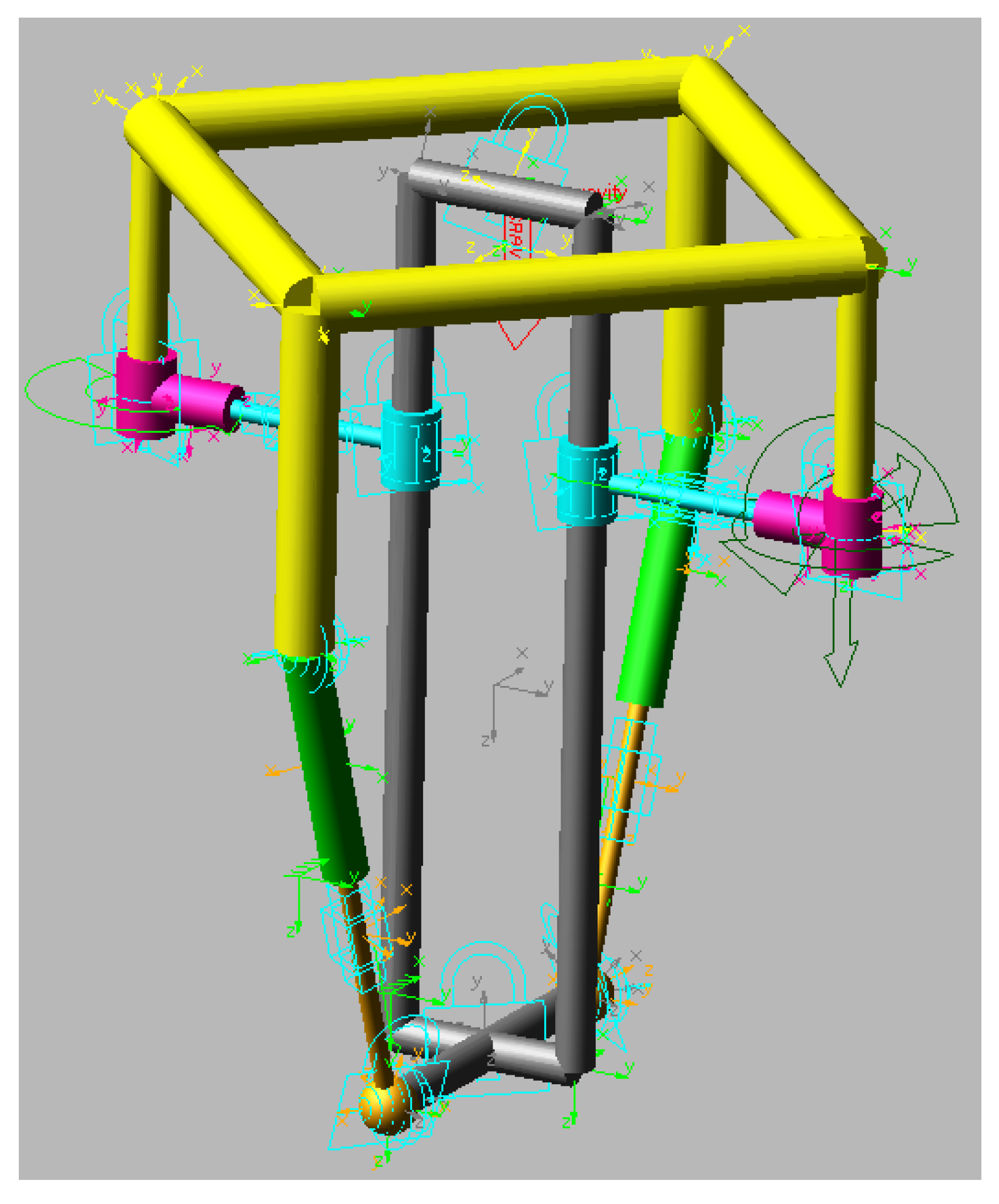
5. Numerical Simulation

In this section, the significance and correctness of the method of kinematic analysis implemented for the parallel manipulator at hand is highlighted by providing some representative numerical examples which cover most of the topics discussed in the contribution. To this end, let us consider that the coordinates of points $A_i(i=1\sim 4)$ are given by

$$\begin{array}{c}\hfill \left\{\begin{array}{c}{A}_1=(0,-200,140)\left[\mathrm{mm}\right],A_2=(0,200,140)\left[\mathrm{mm}\right]\hfill \\ A_3=(-200,0,180)\left[\mathrm{mm}\right],A_4=(200,0,180)\left[\mathrm{mm}\right]\hfill \end{array}\right.\end{array}$$

Furthermore, the parameters of the moving platform are chosen as $d=202.012$ [mm] and $e=100$ [mm]. Note that points $A_1$, $A_2$, $A_3$, and $A_4$ are in different planes to reduce the likelihood of encountering direct kinematic singularities. Furthermore, this arrangement helps maintain the better stability of the parallel manipulator, diminishing the loss of motion or undefined behaviors of the system.

5.1. Displacement

To prove the forward displacement analysis, let us consider that the generalized coordinates of the parallel manipulator are given by

$$\begin{array}{c}\hfill q_1=1.5\left[\mathrm{rad}\right],q_2=140\left[\mathrm{mm}\right],q_3=250\left[\mathrm{mm}\right],q_4=230\left[\mathrm{mm}\right]\end{array}$$

The application of the corresponding algorithm yields three quadratic equations in the unknowns r, h, and $\zeta$ as follows

$$\begin{array}{cc}\hfill & g_1=r^2{\zeta }^2+2.304·{10}^5{\zeta }^2-997.494r{\zeta }^2-28.294r\zeta +r^2-598.496r+70400\hfill \end{array}$$

(40a)

$$\begin{array}{cc}\hfill g_2=& -456.162r{\zeta }^2-80h{\zeta }^2+92204.612{\zeta }^2+h^2{\zeta }^2+r^2{\zeta }^2-417.159r\zeta \hfill \\ & +40804.8\zeta -80.h-285.243r+r^2-28600.187+h^2\hfill \end{array}$$

(40b)

$$\begin{array}{cc}\hfill g_3=& -541.332r{\zeta }^2-80h{\zeta }^2+1.018·{10}^5{\zeta }^2+h^2{\zeta }^2+r^2{\zeta }^2\hfill \\ & +388.864r\zeta -40804.8\zeta -80h-313.253r+r^2-19000.187+h^2\hfill \end{array}$$

(40c)

Equation (40) are solved by resorting to the Sylvester dialytic method of elimination. The method yields twelve solutions, ten complex and two real. The real solutions are as follows

$$\begin{array}{c}\hfill \left\{\begin{array}{c}h=265.705,r=165.570,\zeta =-0.0949,C=(21.120,14.262,395.705),\theta =-0.187\hfill \\ h=-175.705,r=165.570,\zeta =-0.0949,C=(21.120,14.262,-35.705),\theta =-0.187\hfill \end{array}\right.\end{array}$$

To exemplify the inverse displacement analysis, let us consider that the pose of the moving platform is defined by the center $C=(10,20,380)$ [mm] and the orientation angle $\theta =0.2$ [rad]. The application of the algorithm yields the following solution for the inverse position analysis problem

$$\begin{array}{c}\hfill q_1=1.454\left[\mathrm{rad}\right],q_2=130.996\left[\mathrm{mm}\right],q3=228.74\left[\mathrm{mm}\right],q4=223.355\left[\mathrm{mm}\right]\end{array}$$

Unlike the direct position analysis algorithm, the inverse position analysis algorithm is highly efficient due to the closed-form solution available for the latter. In general, the availability of a closed-form solution allows it to bypass iterative computation, making it faster and computationally more efficient. The closed-form nature also lends itself well to real-time applications, where rapid and reliable computation is critical, like in robotic control systems or motion planning.

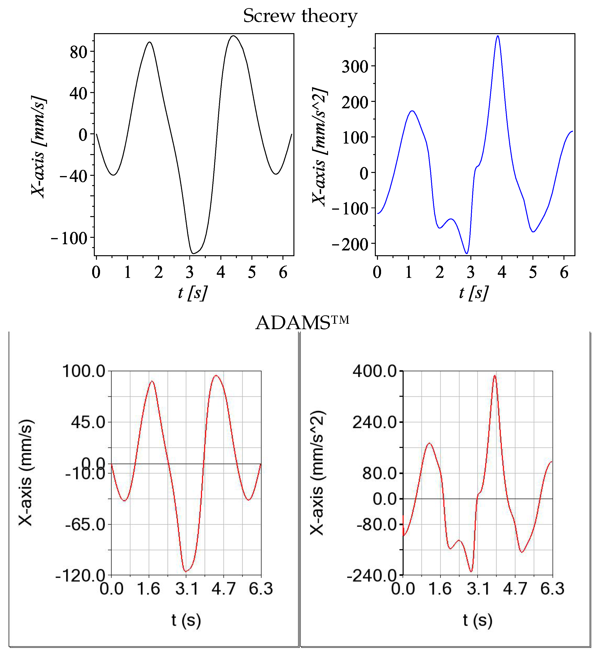
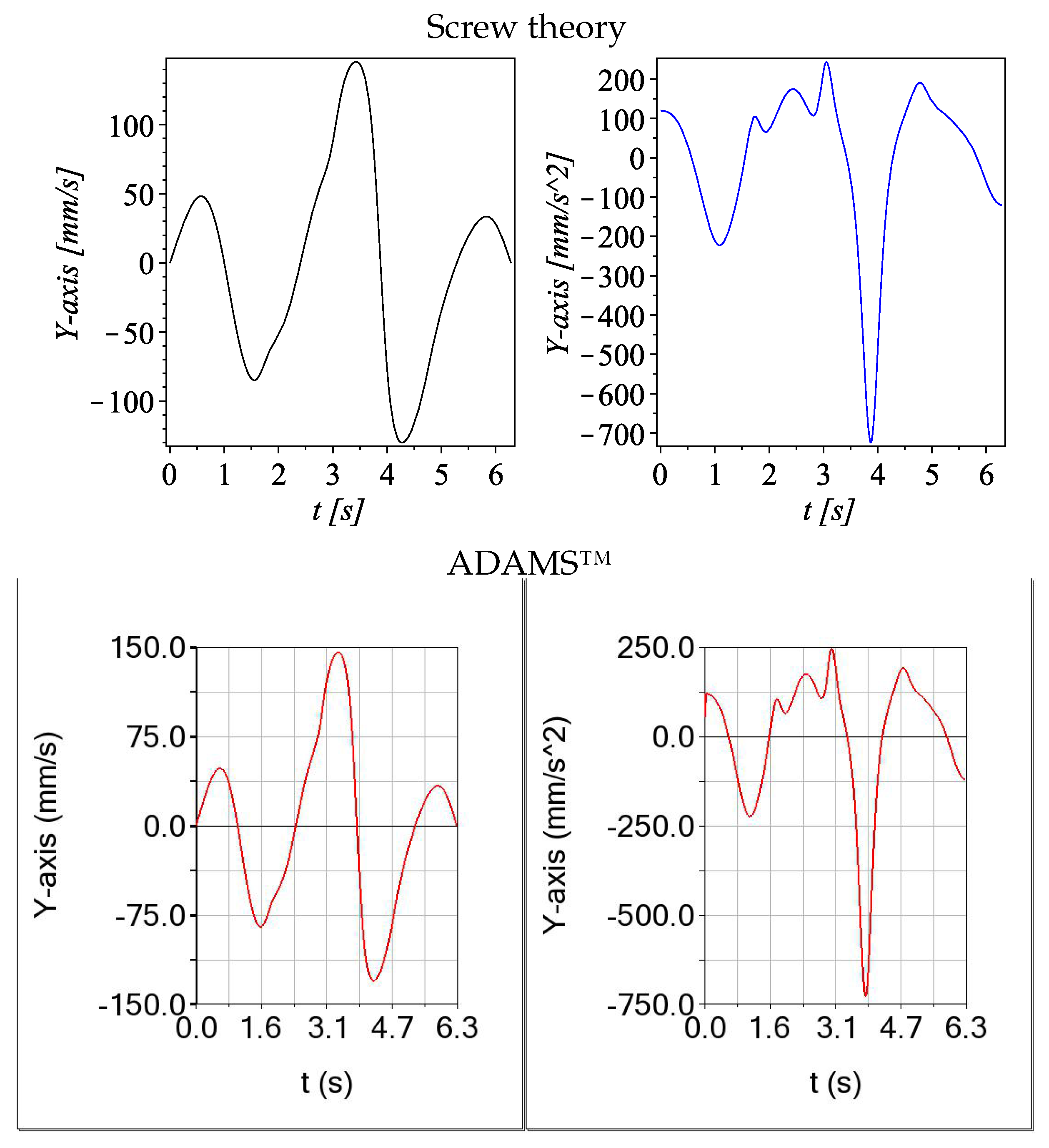
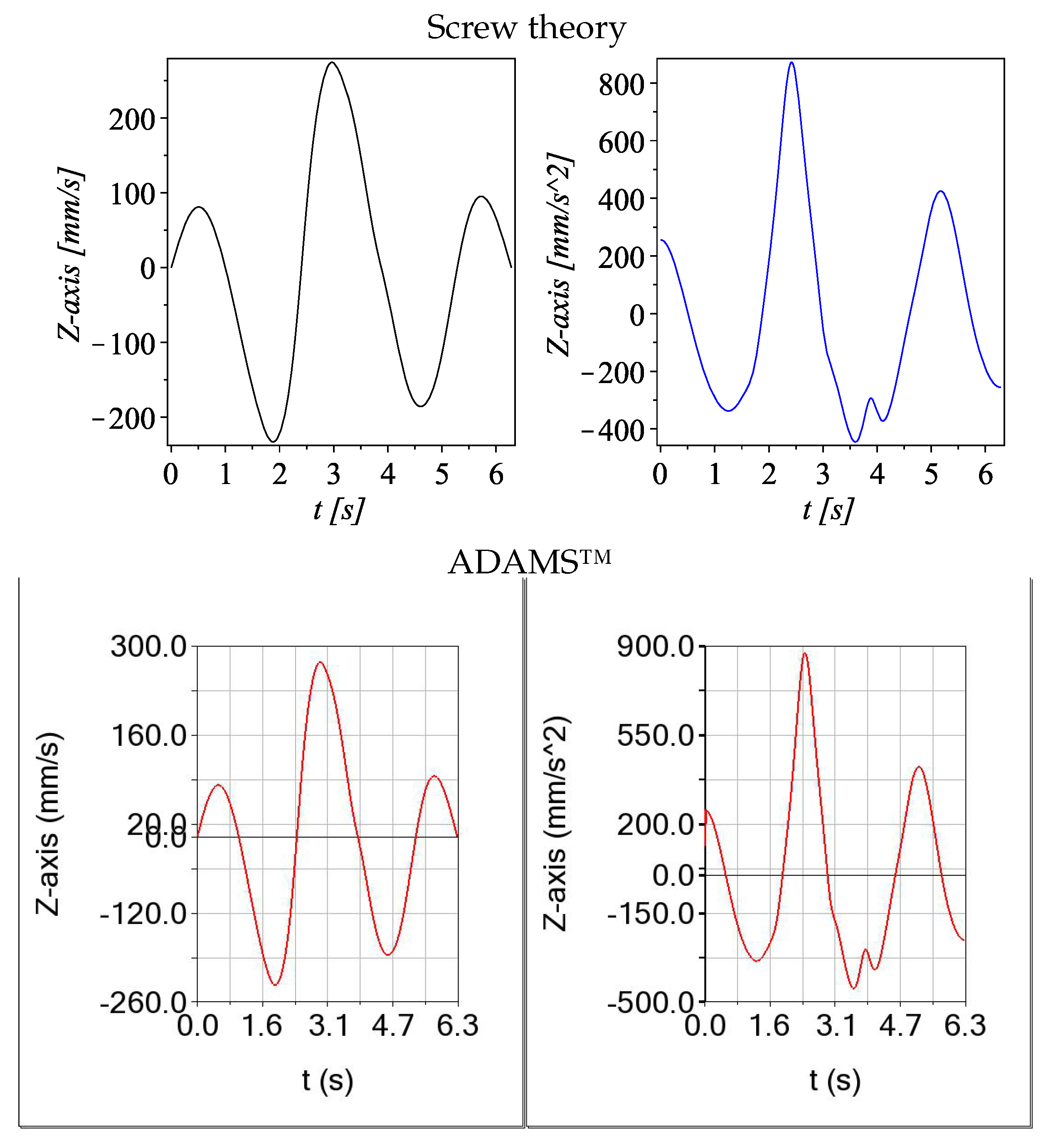
5.2. Velocity and Acceleration—Example 1

Let us consider that the reference configuration of the parallel manipulator is given according to the data provided in

Table 1. Reference configuration of the parallel manipulator.

i	${\mathit{q}}_{\mathit{i}}$	${\mathit{A}}_{\mathit{i}}$ [mm]	${\mathit{B}}_{\mathit{i}}$ [mm]	${\mathit{C}}_{\mathit{i}}$ [mm]
1	$\pi /2$ [rad]	(0, −200, 140)	(0, −50, 140)	(0, −50, 448.994)
2	150 [mm]	(0, 200, 140)	(0, 50, 140)	(0, 50, 448.994)
3	286.631 [mm]	(−200, 0, 180)	—	(−100, 0, 448.994)
4	286.631 [mm]	(200, 0, 180)	—	(100, 0, 448.994)

.

From its reference configuration, the generalized coordinates are governed by periodic functions given by

$$\begin{array}{c}\hfill q_i={\delta }_{i}sin\left(2t\right)sin(t/2)i=1\sim 4\end{array}$$

(41)

where ${\delta }_1=0.25$ [rad], ${\delta }_2=-60$ [mm], ${\delta }_3=100$ [mm], and ${\delta }_4=140$ [mm]. Furthermore, the time t is constrained to the interval $0\le t\le 2\pi$ [s]. From the reference configuration of the parallel manipulator, these periodic functions likely describe how the generalized coordinates change with time. Cyclic motions are a powerful tool to validate instantaneous kinematics in parallel manipulators. By inducing periodic or repetitive motions in the mechanism, it is possible to analyze the velocity and acceleration of the components at various configurations of the robot. This allows for a deeper understanding of how the manipulator behaves kinematically under predictable conditions. The numerical results of the instantaneous angular velocity and acceleration of the moving platform applying the theory of screws are depicted in Figure 6. For a quick comparison and validation, the ADAMS™ plots are placed below the plots obtained with the theory of screws. The ADAMS™ results were obtained from a virtual model developed using the ADAMS™ v2014 dynamic system simulation software; see Figure 7.

On the other hand, the time history of the velocity and acceleration of the center C of the moving platform using the theory of screws and the software ADAMS™ is provided in Figure 8, Figure 9 and Figure 10.

Finally, note how the results of the computation of the instantaneous kinematics of the numerical example 1 using the screw theory reasonably align closely with the results obtained when applying a different approach such as the ADAMS™ v2014 software.

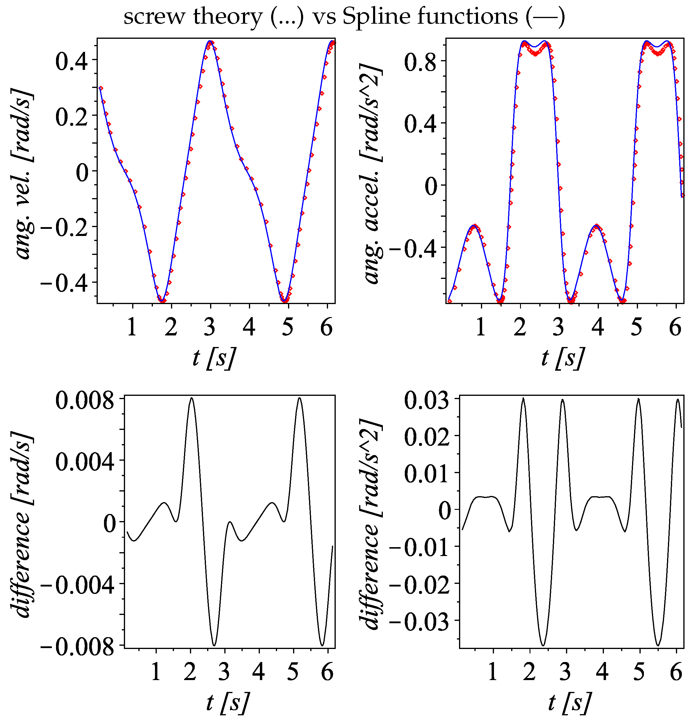
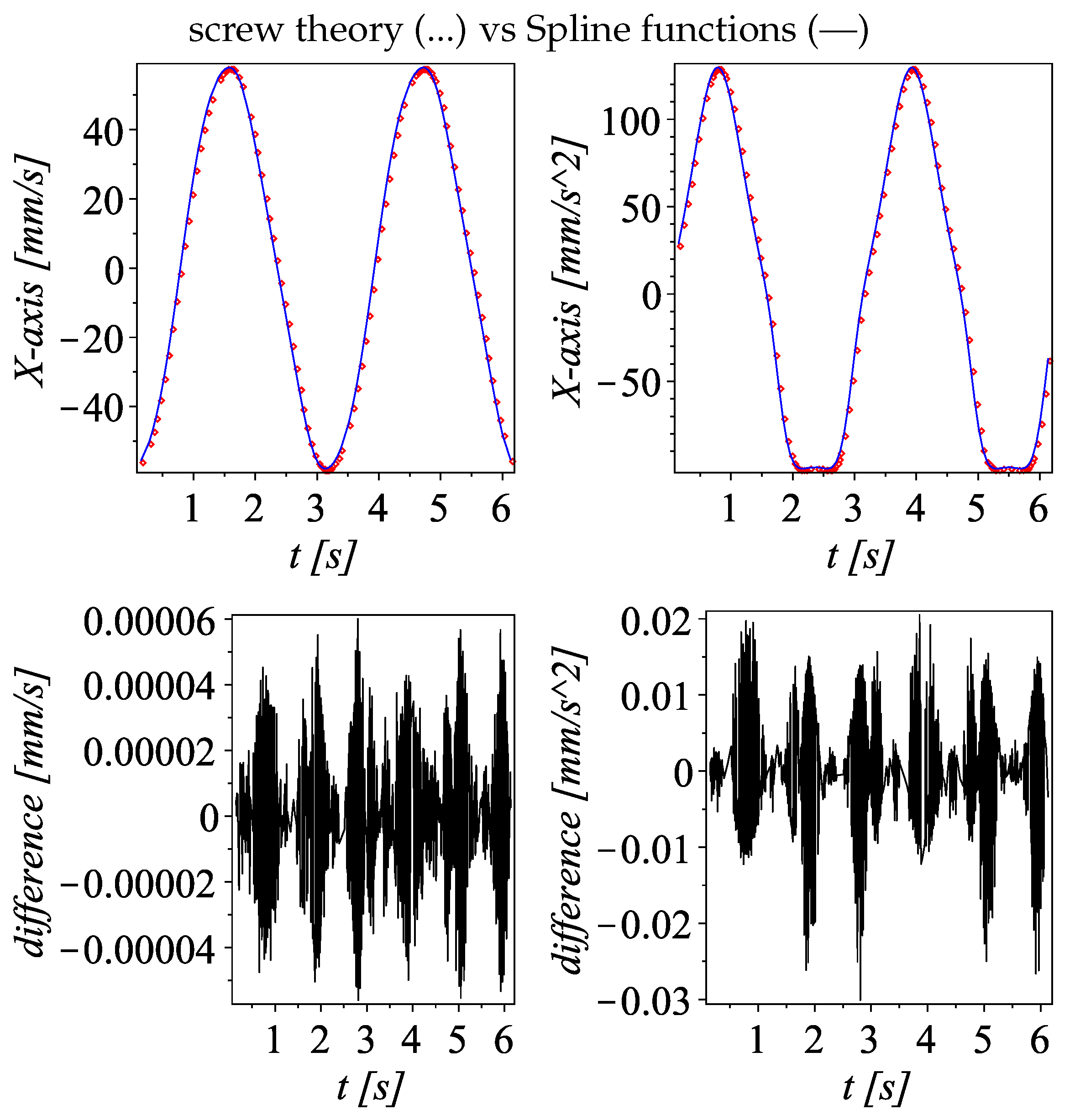
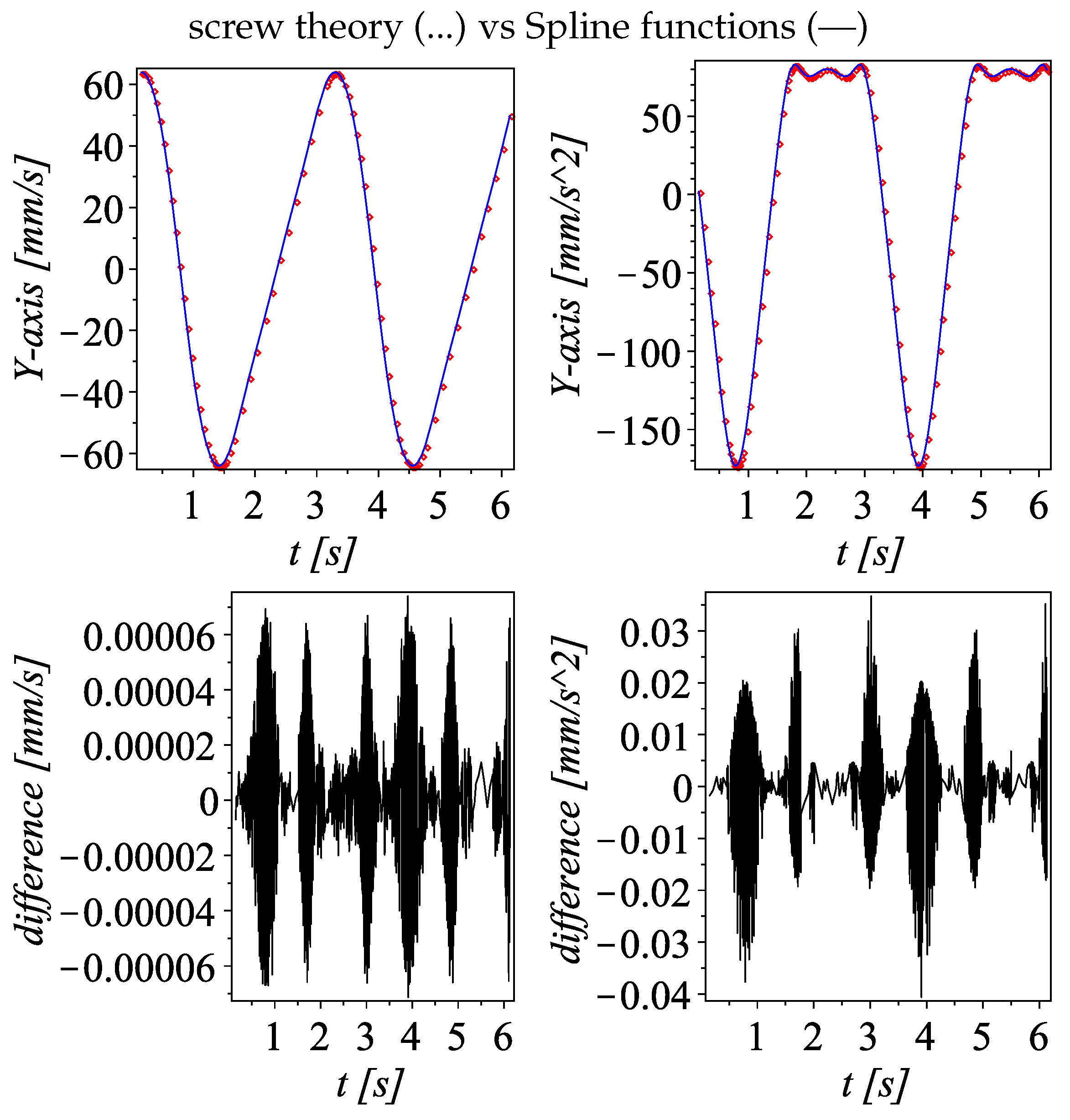
5.3. Velocity and Acceleration—Example 2

To close the numerical applications, a second example also dedicated to illustrating the velocity and acceleration analyses of the parallel manipulator is included. Let us consider that upon the reference configuration of the robot, the generalized coordinates $q_i(i=1\sim 4)$ are controlled by periodic functions given by

$$\begin{array}{c}\hfill q_i={\delta }_{i}sin\left(t\right)cos\left(t\right)\dot{i}=1\sim 4,0\le t\le 2\pi \end{array}$$

(42)

where the parameters ${\delta }_i(i=1\sim 4)$, as well as the other data from example 1, apply to example 2.

The temporal behavior of the kinematic analysis of the moving platform applying the screw theory is summarized in the plots provided in Figure 11, Figure 12, Figure 13 and Figure 14.

To validate the numerical results of example 2, instead of using the ADAMS™software as in example 1, and to reinforce the correctness of the kinematic analysis method using screw theory, an algorithm consisting of the following steps was implemented:

• Formulate the equations of the direct position analysis according to the algorithm described in Section 3.2.
• Since only one solution of the direct position analysis is required, apply a numerical technique such as the Newton–Raphson method to compute the solution for each time step. In the example, it was considered $0\le t\le 2\pi$ with $\Delta t=\pi /180$.
• Obtain time-dependent angular and linear displacement functions of the moving platform using a numerical data fitting method. The Spline command from the (CurveFitting) library of the symbolic mathematics software Maple is particularly efficient for this task due to its ability to smoothly approximate data points.
• Obtain the velocity expressions by applying the time derivatives to the displacement functions generated in the previous point.
• Obtain the acceleration expressions by applying the time derivatives to the velocity functions generated in the previous point.
• Plot the velocity and acceleration expressions to observe trends, periodic behavior, or critical points.

These steps are easy to follow and efficient in generating the angular and linear displacement functions of the moving platform. For example, for the rotation angle $\theta$, the following is obtained:

$$\begin{array}{c}\hfill \theta \left(t\right)=\left\{\begin{array}{c}-6.7668·{10}^{-10}+0.4050t-7.9545t^{3}t<0.1741e-1\hfill \\ 0.8458e-4+0.3977t-0.4165{(t-0.1745e-1)}^2+1.7859{(t-0.1745e-1)}^{3}t<0.0349\hfill \\ 0.4177e-3+0.3848t-0.3229{(t-0.3490e-1)}^2-0.7478{(t-0.3490e-1)}^{3}t<0.0523\hfill \\ ⋮\hfill \\ -2.7488+0.4376t-0.2492{(t-6.2308)}^2+0.1965e-1{(t-6.2308)}^{3}t<6.2482\hfill \\ -2.6946+0.4289t-0.2482{(t-6.2482)}^2-2.5032{(t-6.2482)}^{3}t<6.2657\hfill \\ -2.6261+0.4179t-0.3792{(t-6.2657)}^2+7.2436{(t-6.2657)}^{3}otherwise\hfill \end{array}\right.\end{array}$$

For a quick comparison, the plots obtained with Splines were superimposed with the plots generated with the screw theory. The differences between the two methods are reasonably small, as seen with the difference plots.

6. Conclusions

In this work, a four-legged Schönflies motion generator parallel manipulator, composed of serial kinematic chains with two distinct degrees of freedom, has been introduced. The proposed robot is designed to achieve 3T1R motion (three translations and one rotation) which is particularly advantageous in applications requiring limited yet precise movements. The main findings of the study are summarized as follows:

• Mobility. The global mobility of the mechanism was determined using screw theory, with emphasis on the standard basis that facilitates the 3T1R motion characteristic of Schönflies motion generator mechanisms. This analysis revealed how the constraint systems inherent to each limited-DOF limb govern the interaction of joints and links, which is essential for understanding and computing the effective degrees of freedom available to the robot.
• Displacement analysis. Both forward and inverse position analyses were conducted based on the closure equations of the parallel manipulator. A key observation is the complexity difference between these analyses: the direct position analysis requires solving a system of three quadratic equations, an algebraically demanding task that may yield multiple solutions, whereas the inverse position analysis leads to a single, straightforward solution, making it more suitable for practical implementation.
• Instantaneous kinematics. Compact input–output expressions for velocity and acceleration were derived using screw theory, relating the robot’s input variables (instantaneous generalized coordinates) to the velocity and acceleration of the moving platform relative to the fixed base. This kinematic analysis was complemented by a singularity assessment, which revealed that the proposed manipulator is practically free from singular configurations—an important advantage in robotic applications.
• Numerical examples. Numerical simulations were provided to support the theoretical development. These examples demonstrated the practical applicability of the proposed kinematic methodology. The results were validated by comparison with outputs from alternative tools, including ADAMS™software and data fitting using spline algorithms.
• Although a physical prototype was not constructed, the mechanical design depicted in Figure 1, and validated in ADAMS™, demonstrates feasibility and supports the consideration of realistic scenarios for implementation. The manipulator is well-suited to tasks typically performed by conventional SCARA-type robots, such as the Adept Quattro, and more broadly, Delta-type manipulators.
• Compared to traditional SCARA serial robots, the proposed parallel manipulator demonstrates potential advantages, including greater structural rigidity, improved positioning accuracy, and enhanced robustness. These features make it well-suited for high precision and reliability applications such as electronic component handling, surgical tool positioning, and aeronautical assembly.
• Unlike Delta-type manipulators, which depend on articulated parallelograms and multiple passive links, the proposed 3T1R parallel manipulator employs four serial kinematic chains and eliminates the need for a closed internal loop. This results in a simpler and potentially more efficient mechanical structure, ideal for tasks requiring high stiffness, accurate alignment, and compact rotational motion such as laser cutting, engraving, and other orientation sensitive processes.
• The proposed robot architecture does not include passive limbs; all four limbs are actuated, simplifying control and improving motion precision.

Finally, to the best of the authors’ knowledge, the parallel manipulator presented in this paper has not been previously reported in the literature.

References

1. Clavel, R. Device for the Movement and Positioning of an Element in Space. U.S. Patent No. 4,976,582, 11 December 1990. [Google Scholar]
2. Altuzarra, O.; Şandru, B.; Pinto, C.; Petuya, V. A symmetric parallel Schönflies-motion manipulator for pick-and-place operations. Robotica 2011, 29, 853–862. [Google Scholar] [CrossRef]
3. Cervantes-Sanchez, J.; Rico-Martinez, J.; Perez-Munoz, V. Angularity and axiality of a Schönflies parallel manipulator. Robotica 2016, 34, 2415–2439. [Google Scholar] [CrossRef]
4. Isaksson, M.; Gosselin, C.; Marlow, K. Singularity analysis of a class of kinematically redundant parallel Schönflies motion generators. Mech. Mach. Theory 2017, 112, 172–191. [Google Scholar] [CrossRef]
5. Cao, W.; Yang, D.; Ding, H. A method for stiffness analysis of overconstrained parallel robotic mechanisms with Scara motion. Robot. Comput.-Integr. Manuf. 2018, 49, 426–435. [Google Scholar] [CrossRef]
6. Gallardo-Alvarado, J.; Rodriguez-Castro, R.; Delossantos-Lara, P. Kinematics and dynamics of a 4-PRUR Schönflies parallel manipulator by means of screw theory and the principle of virtual work. Mech. Mach. Theory 2018, 122, 347–360. [Google Scholar] [CrossRef]
7. Kong, X.; Gosselin, C. Type synthesis of 3T1R 4-DOF parallel manipulators based on screw theory. IEEE Trans. Robot. Autom. 2004, 20, 181–190. [Google Scholar] [CrossRef]
8. Guo, S.; Fang, Y.; Qu, H. Type synthesis of 4-DOF nonoverconstrained parallel mechanisms based on screw theory. Robotica 2012, 30, 31–37. [Google Scholar] [CrossRef]
9. Guo, S.; Ye, W.; Qu, H.; Zhang, D.; Fang, Y. A serial of novel four degrees of freedom parallel mechanisms with large rotational workspace. Robotica 2016, 34, 764–776. [Google Scholar] [CrossRef]
10. Zhao, J.S.; Sun, H.L.; Li, H.Y.; Zhao, D.J. Screw Dynamics of a Multibody System by a Schoenflies Manipulator. Appl. Sci. 2023, 13, 9732. [Google Scholar] [CrossRef]
11. Arian, A.; Isaksson, M.; Gosselin, C. Kinematic and dynamic analysis of a novel parallel kinematic Schönflies motion generator. Mech. Mach. Theory 2020, 147, 103629. [Google Scholar] [CrossRef]
12. Wu, G.; Lin, Z.; Zhao, W.; Zhang, S.; Shen, H.; Caro, S. A four-limb parallel Schönflies motion generator with full-circle end-effector rotation. Mech. Mach. Theory 2020, 146, 103711. [Google Scholar] [CrossRef]
13. Meng, Q.; Liu, X.J.; Xie, F. Design and development of a Schönflies-motion parallel robot with articulated platforms and closed-loop passive limbs. Robot. Comput.-Integr. Manuf. 2022, 77, 102352. [Google Scholar] [CrossRef]
14. Urrea, C.; Dominguez, C.; Kern, J. Modeling, design and control of a 4-arm delta parallel manipulator employing type-1 and interval type-2 fuzzy logic-based techniques for precision applications. Robot. Auton. Syst. 2024, 175, 104661. [Google Scholar] [CrossRef]
15. Sanchez-Alonso, R.; Gonzalez-Barbosa, J.J.; Castillo-Castaneda, E.; Gallardo-Alvarado, J. Kinematic analysis of a novel 2(3-RUS) parallel manipulator. Robotica 2016, 34, 2241–2256. [Google Scholar] [CrossRef]
16. Li, Q.; Huang, Z. Mobility Analysis of a Novel 3-5R Parallel Mechanism Family. J. Mech. Des. 2004, 126, 79–82. [Google Scholar] [CrossRef]
17. Dai, J.; Huang, Z.; Lipkin, H. Mobility of Overconstrained Parallel Mechanisms. J. Mech. Des. 2004, 128, 220–229. [Google Scholar] [CrossRef]
18. Lynch, K.; Park, F. Modern Robotics: Mechanics, Planning, and Control; Cambridge University Press: Cambridge, UK, 2017. [Google Scholar]
19. Gallardo-Alvarado, J.; Rodriguez-Castro, R.; Islam, M. Analytical Solution of the Forward Position Analysis of Parallel Manipulators That Generate 3-RS Structures. Adv. Robot. 2008, 22, 215–234. [Google Scholar] [CrossRef]
20. Gallardo-Alvarado, J.; Gallardo-Razo, J. Mechanisms: Kinematic Analysis and Applications in Robotics; Emerging Methodologies and Applications in Modelling, Identification and Control; Academic Press: Cambridge, MA, USA; Elsevier: Amsterdam, The Netherlands, 2022. [Google Scholar]
21. Gallardo-Alvarado, J.; Rico, J. Screw Theory and Helicoidal Fields. In Proceedings of the 25th Biennial Mechanisms Conference, International Design Engineering Technical Conferences and Computers and Information in Engineering Conference, Atlanta, GA, USA, 13–16 September 1998; Volume 1B, p. V01BT01A007. [Google Scholar] [CrossRef]
Figure 1. The proposed Schönflies motion generator parallel manipulator.
Mathematics 13 02291 g001
Figure 2. Dimensional parameters and coordinates of the parallel manipulator.
Mathematics 13 02291 g002
Figure 3. Screw system of the RPC kinematic chain.
Mathematics 13 02291 g003
Figure 4. Screws of two limbs and reciprocal lines of the parallel manipulator.
Mathematics 13 02291 g004
Figure 5. Two direct singularities of the parallel manipulator.
Mathematics 13 02291 g005
Figure 6. Time history of the angular velocity and acceleration of the moving platform. Example 1.
Mathematics 13 02291 g006
Figure 7. Virtual model in ADAMS™. Example 1.
Mathematics 13 02291 g007
Figure 8. Time history of the velocity in the X-axis of point C. Example 1.
Mathematics 13 02291 g008
Figure 9. Time history of the velocity in the Y-axis of point C. Example 1.
Mathematics 13 02291 g009
Figure 10. Time history of the velocity in the Z-axis of point C. Example 1.
Mathematics 13 02291 g010
Figure 11. Time history of the angular velocity and acceleration of the moving platform. Example 2.
Mathematics 13 02291 g011
Figure 12. Time history of the velocity in the X-axis of point C. Example 2.
Mathematics 13 02291 g012
Figure 13. Time history of the velocity in the Y-axis of point C. Example 2.
Mathematics 13 02291 g013
Figure 14. Time history of the velocity in the Z-axis of point C. Example 2.
Mathematics 13 02291 g014