
DLPLSR: Dual Label Propagation-Driven Least Squares Regression with Feature Selection for Semi-Supervised Learning


Abstract
1. Introduction
- Dual label propagation mechanism: The global structure is preserved via the fuzzy graph, while the adaptive manifold regularization captures local geometric relationships among samples. Benefiting from this design, a dual label propagation mechanism is established to enable effective and consistent knowledge transfer from labeled to unlabeled data.
- Dual feature selection mechanism: An orthogonal projection is employed to preserve feature diversity and maximize information retention, while an ℓ2,1-norm regularization imposes structured sparsity to eliminate irrelevant dimensions. This dual feature selection mechanism enhances the robustness and discriminant capability of the learned representations under limited supervision.
- Pseudo-labels free framework: The proposed framework discards the use of pseudo-labels typically required in semi-supervised LSR models, thereby avoiding performance degradation caused by low-quality supervision. Instead, it transfers supervision from labeled to unlabeled data solely based on structural relationships, which are fully captured through fuzzy graph similarity and manifold regularization.
- End-to-end unified optimization: The model eliminates manual intervention and integrates all components into a single unified objective. It supports fully end-to-end optimization, allowing all modules to be jointly trained via an alternating strategy with closed-form solutions and guaranteed convergence.
2. Preliminaries and Related Works
2.1. Notations and Definitions
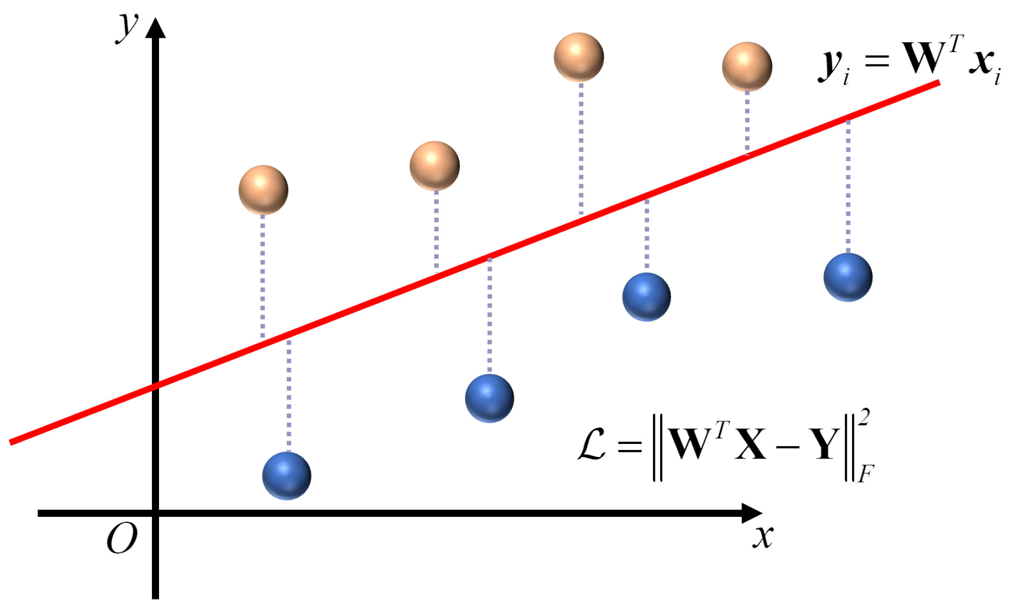
2.2. Least Squares Regression
2.3. Semi-Supervised LSR
2.4. Fuzzy Graph and Its Derived Clustering
3. Model Description
3.1. Pseudo-Label-Free Semi-LSR with LP Based on Manifold
3.2. Dual Label Propagation
3.3. Dual Feature Selection
4. Optimization Strategy
4.1. Algorithm Implementation
| Algorithm 1 Generalized power iteration (GPI) [46] for Equation (12). |
| Input: Symmetric matrix , matrix . Output: Orthogonal matrix . 1: Initialize . 2: repeat 3: Compute , 4: Perform SVD: , 5: Update . 6: until convergence 7: return |
| Algorithm 2 DLPLSR: Dual label propagation-driven with feature selection regression for semi-supervised classification. |
| Input: Labeled data , unlabeled data , hyperparameters . Output: Final classifier . 1: Initialize . 2: Calculate . 3: repeat 4: Compute by Equation (17). 5: Update by Equation (16) according to [47]. 6: Calculate and by Equations (13) and (14). 7: Update according to Algorithm 1. 8: until convergence |
4.2. Complexity Analysis
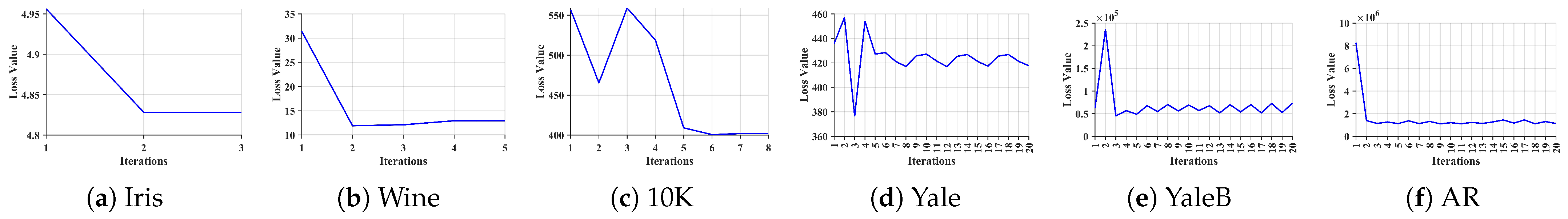
4.3. Convergence Analysis
5. Experiments
5.1. Datasets
5.2. Baseline Methods
- RSSLSR (robust semi-supervised least squares regression using ℓ2,p-norm minimization) [33]: A biased regression model in which each training sample is associated with a learnable weight. It adopts the ℓ2,p-norm to compute the classification loss, thereby enhancing robustness against outliers and label noise.
- SFS_BLL (semi-supervised feature selection with binary label learning) [29]: Performs discriminative feature selection in a binary hashing code space, enhancing class separability. However, its two-stage manual graph construction process may limit adaptability and increase sensitivity to noise.
- DSLSR (discriminative sparse least squares regression) [24]: Enhances the discriminability of the regression space by employing a coordinate relaxation matrix to enlarge the distance between inter-class samples, while imposing sparsity constraints on regression features for more compact representation.
- RER (robust embedding regression) [30]: Constructs an adaptive graph based on self-expressiveness, and evaluates the regression error using the nuclear norm, which captures the global low-rank structure of the error matrix from a holistic perspective. This enhances the model’s robustness against noise and outliers.
- DRLSR (discriminative and robust least squares regression) [34]: Constructs an adaptive anchor-based graph and performs label propagation via the fuzzy membership matrix derived from classical fuzzy clustering, so enhances the model’s robustness and discriminability under semi-supervised scenarios.
- AGLSOFS_N (adaptive orthogonal semi-supervised feature selection with reliable label matrix learning_norm) [31]: Incorporates confidence-based label learning to control inter-class overlap, employs orthogonal projection to enhance feature discriminability, and introduces a Frobenius norm regularization term to facilitate adaptive graph construction.
- AGLSOFS_E (adaptive orthogonal semi-supervised feature selection with reliable label matrix learning_entropy) [31]: Similar in overall structure to AGLSOFS_N, but replaces the Frobenius norm with an entropy regularization term to achieve adaptive graph construction, resulting in a denser similarity structure.
5.3. Evaluation Metrics
- TP (True Positive): Positive samples correctly predicted as positive.
- FP (False Positive): Negative samples incorrectly predicted as positive.
- TN (True Negative): Negative samples correctly predicted as negative.
- FN (False Negative): Positive samples incorrectly predicted as negative.
5.4. Configurations
5.4.1. Testing Configuration
5.4.2. Semi-Supervised Configuration
5.4.3. Hyperparameters Configurations
5.5. Comparison Experiments
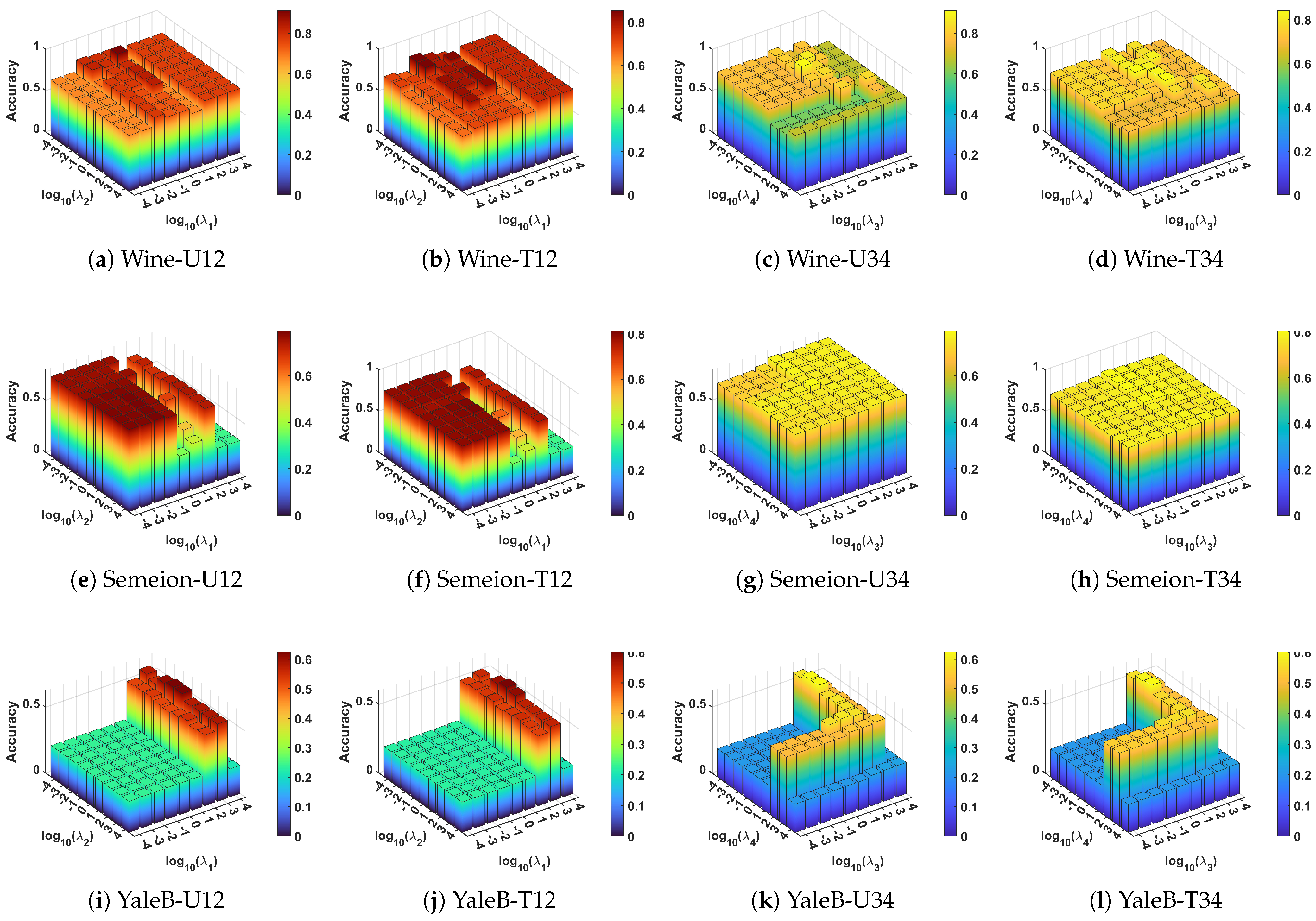
5.6. Parameter Sensitivity
5.7. Ablation Study
5.8. Visualization Analysis
5.9. Real-World Applications Experiments
6. Discussion
Author Contributions
Funding
Data Availability Statement
Acknowledgments
Conflicts of Interest
References
- Kotsiantis, S.B.; Zaharakis, I.D.; Pintelas, P.E. Machine learning: A review of classification and combining techniques. Artif. Intell. Rev. 2006, 26, 159–190. [Google Scholar] [CrossRef]
- Sen, P.C.; Hajra, M.; Ghosh, M. Supervised classification algorithms in machine learning: A survey and review. In Emerging Technology in Modelling and Graphics: Proceedings of IEM Graph 2018; Springer Nature: Singapore, 2020; pp. 99–111. [Google Scholar]
- Chen, L.; Li, S.; Bai, Q.; Yang, J.; Jiang, S.; Miao, Y. Review of image classification algorithms based on convolutional neural networks. Remote Sens. 2021, 13, 4712. [Google Scholar] [CrossRef]
- Zhang, S. Challenges in KNN classification. IEEE Trans. Knowl. Data Eng. 2021, 34, 4663–4675. [Google Scholar] [CrossRef]
- Xie, J.; Xiang, X.; Xia, S.; Jiang, L.; Wang, G.; Gao, X. Mgnr: A multi-granularity neighbor relationship and its application in knn classification and clustering methods. IEEE Trans. Pattern Anal. Mach. Intell. 2024, 46, 7956–7972. [Google Scholar] [CrossRef] [PubMed]
- Chandra, M.A.; Bedi, S. Survey on SVM and their application in image classification. Int. J. Inf. Technol. 2021, 13, 1–11. [Google Scholar] [CrossRef]
- Zhang, Y.; Liu, L.; Qiao, Q.; Li, F. A Lie group Laplacian Support Vector Machine for semi-supervised learning. Neurocomputing 2025, 630, 129728. [Google Scholar] [CrossRef]
- He, K.; Zhang, X.; Ren, S.; Sun, J. Deep residual learning for image recognition. In Proceedings of the IEEE Conference on Computer Vision and Pattern Recognition (CVPR), Vegas, NV, USA, 27–30 June 2016; pp. 770–778. [Google Scholar]
- Shafiq, M.; Gu, Z. Deep residual learning for image recognition: A survey. Appl. Sci. 2022, 12, 8972. [Google Scholar] [CrossRef]
- Liu, Z.; Lin, Y.; Cao, Y.; Hu, H.; Wei, Y.; Zhang, Z.; Lin, S.; Guo, B. Swin transformer: Hierarchical vision transformer using shifted windows. In Proceedings of the IEEE/CVF International Conference on Computer Vision (CVPR), Nashville, TN, USA, 20–25 June 2021; pp. 10012–10022. [Google Scholar]
- Han, K.; Wang, Y.; Chen, H.; Chen, X.; Guo, J.; Liu, Z.; Tang, Y.; Xiao, A.; Xu, C.; Xu, Y.; et al. A survey on vision transformer. IEEE Trans. Pattern Anal. Mach. Intell. 2022, 45, 87–110. [Google Scholar] [CrossRef] [PubMed]
- Jain, A.; Patel, H.; Nagalapatti, L.; Gupta, N.; Mehta, S.; Guttula, S.; Mujumdar, S.; Afzal, S.; Sharma Mittal, R.; Munigala, V. Overview and importance of data quality for machine learning tasks. In Proceedings of the 26th ACM SIGKDD International Conference on Knowledge Discovery & Data Mining (KDD), Virtual, 6–10 July 2020; pp. 3561–3562. [Google Scholar]
- Van Engelen, J.E.; Hoos, H.H. A survey on semi-supervised learning. Mach. Learn. 2020, 109, 373–440. [Google Scholar] [CrossRef]
- Han, K.; Sheng, V.S.; Song, Y.; Liu, Y.; Qiu, C.; Ma, S.; Liu, Z. Deep semi-supervised learning for medical image segmentation: A review. Expert Syst. Appl. 2024, 245, 123052. [Google Scholar] [CrossRef]
- Zhou, Z.H.; Zhou, Z.H. Semi-supervised learning. In Machine Learning; Springer: Berlin/Heidelberg, Germany, 2021; Chapter 13; pp. 315–341. [Google Scholar]
- Bennett, K.; Demiriz, A. Semi-supervised support vector machines. Adv. Neural Inf. Process. Syst. NIPS 1998, 11, 368–374. [Google Scholar]
- Belkin, M.; Niyogi, P.; Sindhwani, V. Manifold regularization: A geometric framework for learning from labeled and unlabeled examples. J. Mach. Learn. Res. 2006, 7, 2399–2434. [Google Scholar]
- Nie, F.; Shi, S.; Li, X. Semi-supervised learning with auto-weighting feature and adaptive graph. IEEE Trans. Knowl. Data Eng. 2019, 32, 1167–1178. [Google Scholar] [CrossRef]
- Qiao, X.; Chen, C.; Wang, W.; Peng, Q.; Ghafar, A. Efficient ℓ2,1-norm graph for robust semi-supervised classification. Pattern Recognit. 2025, 169, 111890. [Google Scholar] [CrossRef]
- Jia, Y.; Kwong, S.; Hou, J.; Wu, W. Semi-supervised non-negative matrix factorization with dissimilarity and similarity regularization. IEEE Trans. Neural Netw. Learn. Syst. 2019, 31, 2510–2521. [Google Scholar] [CrossRef] [PubMed]
- Yuan, A.; You, M.; He, D.; Li, X. Convex non-negative matrix factorization with adaptive graph for unsupervised feature selection. IEEE Trans. Cybern. 2020, 52, 5522–5534. [Google Scholar] [CrossRef] [PubMed]
- Chen, X.; Yuan, G.; Nie, F.; Huang, J.Z. Semi-supervised Feature Selection via Rescaled Linear Regression. In Proceedings of the International Joint Conference on Artificial Intelligence (IJCAI), Melbourne, Australia, 19–25 August 2017; Volume 2017, pp. 1525–1531. [Google Scholar]
- Xu, S.; Dai, J.; Shi, H. Semi-supervised feature selection based on least square regression with redundancy minimization. In Proceedings of the 2018 International Joint Conference on Neural Networks (IJCNN), Rio de Janeiro, Brazil, 8–13 July 2018; pp. 1–8. [Google Scholar]
- Liu, Z.; Lai, Z.; Ou, W.; Zhang, K.; Huo, H. Discriminative sparse least square regression for semi-supervised learning. Inf. Sci. 2023, 636, 118903. [Google Scholar] [CrossRef]
- Zhong, W.; Chen, X.; Yuan, G.; Li, Y.; Nie, F. Semi-supervised feature selection with adaptive discriminant analysis. In Proceedings of the AAAI Conference on Artificial Intelligence, Honolulu, HI, USA, 27 January–1 February 2019; Volume 33, pp. 10083–10084. [Google Scholar]
- Wang, C.; Chen, X.; Yuan, G.; Nie, F.; Yang, M. Semisupervised feature selection with sparse discriminative least squares regression. IEEE Trans. Cybern. 2021, 52, 8413–8424. [Google Scholar] [CrossRef] [PubMed]
- Nie, F.; Xu, D.; Tsang, I.W.H.; Zhang, C. Flexible manifold embedding: A framework for semi-supervised and unsupervised dimension reduction. IEEE Trans. Image Process. 2010, 19, 1921–1932. [Google Scholar] [CrossRef] [PubMed]
- Qiu, S.; Nie, F.; Xu, X.; Qing, C.; Xu, D. Accelerating flexible manifold embedding for scalable semi-supervised learning. IEEE Trans. Circuits Syst. Video Technol. 2018, 29, 2786–2795. [Google Scholar] [CrossRef]
- Shi, D.; Zhu, L.; Li, J.; Cheng, Z.; Liu, Z. Binary label learning for semi-supervised feature selection. IEEE Trans. Knowl. Data Eng. 2023, 35, 2299–2312. [Google Scholar] [CrossRef]
- Bao, J.; Kudo, M.; Kimura, K.; Sun, L. Robust embedding regression for semi-supervised learning. Pattern Recognit. 2024, 145, 109894. [Google Scholar] [CrossRef]
- Liao, H.; Chen, H.; Yin, T.; Horng, S.J.; Li, T. Adaptive orthogonal semi-supervised feature selection with reliable label matrix learning. Inf. Process. Manag. 2024, 61, 103727. [Google Scholar] [CrossRef]
- Zhang, H.; Gong, M.; Nie, F.; Li, X. Unified dual-label semi-supervised learning with top-k feature selection. Neurocomputing 2022, 501, 875–888. [Google Scholar] [CrossRef]
- Wang, J.; Xie, F.; Nie, F.; Li, X. Robust supervised and semisupervised least squares regression using ℓ2,p-norm minimization. IEEE Trans. Neural Netw. Learn. Syst. 2022, 34, 8389–8403. [Google Scholar] [CrossRef] [PubMed]
- Wang, J.; Chen, C.; Nie, F.; Li, X. Discriminative and robust least squares regression for semi-supervised image classification. Neurocomputing 2024, 575, 127316. [Google Scholar] [CrossRef]
- McDonald, G.C. Ridge regression. Wiley Interdiscip. Rev. Comput. Stat. 2009, 1, 93–100. [Google Scholar] [CrossRef]
- Varaprasad, S.; Goel, T.; Tanveer, M.; Murugan, R. An effective diagnosis of schizophrenia using kernel ridge regression-based optimized RVFL classifier. Appl. Soft Comput. 2024, 157, 111457. [Google Scholar] [CrossRef]
- Ranstam, J.; Cook, J.A. LASSO regression. J. Br. Surg. 2018, 105, 1348. [Google Scholar] [CrossRef]
- Wang, S.; Chen, Y.; Cui, Z.; Lin, L.; Zong, Y. Diabetes risk analysis based on machine learning LASSO regression model. J. Theory Pract. Eng. Sci. 2024, 4, 58–64. [Google Scholar]
- Zhang, Z.; Lai, Z.; Xu, Y.; Shao, L.; Wu, J.; Xie, G.S. Discriminative elastic-net regularized linear regression. IEEE Trans. Image Process. 2017, 26, 1466–1481. [Google Scholar] [CrossRef] [PubMed]
- Amini, F.; Hu, G. A two-layer feature selection method using genetic algorithm and elastic net. Expert Syst. Appl. 2021, 166, 114072. [Google Scholar] [CrossRef]
- Zhu, X.; Ghahramani, Z.; Lafferty, J.D. Semi-supervised learning using gaussian fields and harmonic functions. In Proceedings of the 20th International Conference on MACHINE Learning (ICML-03), Washington, DC, USA, 21–24 August 2003; pp. 912–919. [Google Scholar]
- Zhou, D.; Bousquet, O.; Lal, T.; Weston, J.; Schölkopf, B. Learning with local and global consistency. Adv. Neural Inf. Process. Syst. NIPS 2003, 16, 1–8. [Google Scholar]
- Chen, X.; Yuan, G.; Nie, F.; Ming, Z. Semi-supervised feature selection via sparse rescaled linear square regression. IEEE Trans. Knowl. Data Eng. 2018, 32, 165–176. [Google Scholar] [CrossRef]
- Qi, X.; Zhang, H.; Nie, F. Discriminative Semi-Supervised Feature Selection Via a Class-Credible Pseudo-Label Learning Framework. In Proceedings of the ICASSP 2024-2024 IEEE International Conference on Acoustics, Speech and Signal Processing (ICASSP), Seoul, Republic of Korea, 14–19 April 2024; pp. 6895–6899. [Google Scholar]
- Shi, Z.; Chen, L.; Ding, W.; Zhong, X.; Wu, Z.; Chen, G.Y.; Zhang, C.; Wang, Y.; Chen, C.L.P. IFKMHC: Implicit Fuzzy K-Means Model for High-Dimensional Data Clustering. IEEE Trans. Cybern. 2024, 54, 7955–7968. [Google Scholar] [CrossRef] [PubMed]
- Nie, F.; Zhang, R.; Li, X. A generalized power iteration method for solving quadratic problem on the stiefel manifold. Sci. China Inf. Sci. 2017, 60, 1–10. [Google Scholar] [CrossRef]
- Huang, J.; Nie, F.; Huang, H. A new simplex sparse learning model to measure data similarity for clustering. In Proceedings of the IJCAI, Buenos Aires, Argentina, 25–31 July 2015; pp. 3569–3575. [Google Scholar]
- Xu, C.; Si, J.; Guan, Z.; Zhao, W.; Wu, Y.; Gao, X. Reliable conflictive multi-view learning. In Proceedings of the AAAI Conference on Artificial Intelligence, Vancouver, BC, Canada, 20–27 February 2024; Volume 38, pp. 16129–16137. [Google Scholar]
- Shi, Z.; Chen, L.; Ding, W.; Zhang, C.; Wang, Y. Parameter-free robust ensemble framework of fuzzy clustering. IEEE Trans. Fuzzy Syst. 2023, 31, 4205–4219. [Google Scholar] [CrossRef]
- Shi, Z.; Luo, Y.; Liu, X.; Chen, L.; Ding, W.; Zhong, X.; Wu, Z.; Philip Chen, C.L. MGL-FBLS: Multi-Granularity Label-Driven Feature Enhanced Broad Learning System for Semi-Supervised Classification. IEEE Trans. Emerg. Top. Comput. Intell. 2025; early access. [Google Scholar] [CrossRef]


| Type | UCI | Handwriting | Objects | Faces | ||||||||||
|---|---|---|---|---|---|---|---|---|---|---|---|---|---|---|
| Dataset | Iris | Wine | USPS | 2k2k | 10k | Semeion | COIL20 | COIL100 | ORL | Jaffe | PIX10 | Yale | YaleB | AR |
| No. | ① | ② | ③ | ④ | ⑤ | ⑥ | ⑦ | ⑧ | ⑨ | ⑩ | ❶ | ❷ | ❸ | ❹ |
| Features | 4 | 13 | 16 × 16 | 28 × 28 | 28 × 28 | 16 × 16 | 32 × 32 | 32×32 | 32 × 32 | 32 × 32 | 100 × 100 | 32 × 32 | 32 × 32 | 55 × 40 |
| Instances | 150 | 178 | 9298 | 4000 | 10,000 | 1593 | 1440 | 7200 | 400 | 213 | 100 | 165 | 2414 | 2600 |
| Classes | 3 | 3 | 10 | 10 | 10 | 10 | 20 | 100 | 40 | 10 | 10 | 15 | 38 | 100 |
| Capacity | 50 | 48, 59, 71 | 708–1553 | 359–454 | 863–1127 | 155–162 | 72 | 72 | 10 | 20–23 | 10 | 11 | 59–64 | 26 |
| Methods | Label Propagation | Feature Selection | Samples’ Relationship | Biased Regression | Pseudo-Labels Learning | Number of Parameters | Solver | Highlights |
|---|---|---|---|---|---|---|---|---|
| RSSLSR [33] | No special | No special | No special | ✓ | ✓ | 3 | Alternative iterations | Sample-wise weights |
| SFS_BLL [29] | Pre-KNN | Sparse | Local | ✗ | ✓ | 5 | ADMM | Binary hash |
| DSLSR [24] | Pre-KNN | No special | Local | ✓ | ✓ | 5 | ADMM | Discriminant enhanced |
| RER [30] | Self-expression | Sparse | Global | ✓ | ✓ | 3 | ADMM | Robustness enhanced |
| DRLSR [34] | Fuzzy clustering | No special | Global | ✓ | ✓ | 3 | Alternative iterations | Anchor graph |
| AGLSOFS_N [31] | Adaptive manifold | Orthogonal + Sparse | Local | ✗ | ✓ | 4 | Alternative iterations | Reliable label |
| AGLSOFS_E [31] | Adaptive manifold | Orthogonal + Sparse | Local | ✗ | ✓ | 4 | Alternative iterations | Reliable label |
| DLPLSR | Fuzzy clustering + Adaptive manifold | Orthogonal + Sparse | Local + Global | ✗ | ✗ | 4 | Alternative iterations | Dual-LP Pseudo-label-free |
| Prediction Strategy | RSSLSR [33] | SFS_BLL [29] | DSLSR [24] | RER [30] | DRLSR [34] | AGLSOFS_N [31] | AGLSOFS_E [31] | DLPLSR |
|---|---|---|---|---|---|---|---|---|
| Unlabeled specified | ✗ | ✗ | ✗ | Pseudo labels | Pseudo labels | ✗ | ✗ | 1-NN |
| Unlabeled in experiments | Pseudo labels | 1-NN | 1-NN | Pseudo labels | Pseudo labels | 1-NN | Pseudo labels | 1-NN |
| Testing in experiments | 1-NN | 1-NN | 1-NN | 1-NN | 1-NN | 1-NN | 1-NN | 1-NN |
| Opts | ① | ② | ③ | ④ | ⑤ | ⑥ | ⑦ | ⑧ | ⑨ | ⑩ | ❶ | ❷ | ❸ | ❹ |
|---|---|---|---|---|---|---|---|---|---|---|---|---|---|---|
| 0.0001 | 0.1 | 10 | 0.1 | 0.01 | 1 | 10 | 100 | 10 | 1000 | 10 | 1 | 0.01 | 0.1 | |
| 0.0001 | 1 | 1 | 1 | 0.001 | 1 | 0.0001 | 100 | 100 | 10 | 100 | 1 | 100 | 10,000 | |
| 0.0001 | 0.001 | 1000 | 100 | 1 | 10 | 10 | 100 | 0.0001 | 10,000 | 1000 | 10 | 0.1 | 10 | |
| 0.0001 | 1 | 1 | 0.0001 | 0.1 | 0.01 | 100 | 100 | 100 | 10,000 | 10 | 10 | 1000 | 10,000 |
| Unlabeled | Testing | |||||||||||||||
|---|---|---|---|---|---|---|---|---|---|---|---|---|---|---|---|---|
| RSSLSR | SFS_BLL | DSLSR | RER | DRLSR | AGLSOFS | AGLSOFSE | DLPLSR | RSSLSR | SFS | DSLSR | RER | DRLSR | AGLSOFS_N | AGLSOFS_E | DLPLSR | |
| Iris | 73.13 (8) | 85.07 (6) | 95.52 (1) | 92.54 (3) | 89.55 (4) | 89.55 (4) | 74.63 (7) | 95.52 (1) | 100.00 (1) | 96.00 (6) | 100.00 (1) | 100.00 (1) | 96.00 (6) | 94.67 (8) | 98.67 (5) | 100.00 (1) |
| Wine | 70.00 (6) | 73.75 (4) | 76.25 (3) | 71.25 (5) | 62.50 (7) | 78.75 (2) | 43.75 (8) | 91.25 (1) | 70.79 (5) | 70.79 (5) | 83.15 (3) | 70.79 (5) | 62.92 (8) | 84.27 (1) | 76.40 (4) | 84.27 (1) |
| USPS | 86.66 (6) | 53.91 (8) | 89.24 (3) | 95.70 (1) | 89.77 (2) | 87.52 (5) | 75.86 (7) | 87.91 (4) | 88.30 (2) | 54.33 (8) | 88.19 (3) | 82.66 (7) | 88.34 (1) | 86.26 (5) | 85.76 (6) | 86.75 (4) |
| 2k2k | 74.17 (6) | 76.00 (4) | 75.28 (5) | 86.67 (1) | 65.44 (7) | 78.28 (2) | 64.67 (8) | 77.39 (3) | 79.25 (3) | 76.90 (6) | 77.55 (5) | 74.40 (7) | 65.50 (8) | 79.65 (2) | 78.40 (4) | 79.95 (1) |
| 10k | 81.42 (5) | 81.04 (6) | 84.16 (4) | 93.36 (1) | 79.40 (7) | 84.36 (3) | 70.73 (8) | 85.11 (2) | 84.30 (3) | 81.04 (6) | 83.44 (4) | 78.74 (8) | 80.02 (7) | 85.74 (1) | 83.26 (5) | 84.66 (2) |
| Semeion | 69.83 (5) | 53.91 (7) | 75.98 (4) | 79.19 (1) | 32.26 (8) | 77.93 (3) | 61.45 (6) | 79.19 (1) | 75.28 (4) | 54.33 (7) | 71.27 (5) | 69.89 (6) | 34.76 (8) | 80.68 (1) | 78.04 (3) | 80.18 (2) |
| COIL20 | 79.17 (6) | 81.48 (4) | 84.10 (2) | 86.11 (1) | 62.19 (8) | 79.94 (5) | 68.67 (7) | 82.56 (3) | 80.00 (5) | 79.58 (6) | 83.61 (1) | 80.28 (4) | 62.78 (8) | 78.19 (7) | 81.53 (3) | 83.47 (2) |
| COIL100 | 56.23 (6) | 68.49 (4) | 72.19 (2) | 75.49 (1) | 53.55 (7) | 67.87 (5) | 47.59 (8) | 68.77 (3) | 60.17 (7) | 66.03 (2) | 69.17 (1) | 64.06 (6) | 50.11 (8) | 64.97 (4) | 64.47 (5) | 65.92 (3) |
| ORL | 24.44 (2) | 9.44 (8) | 21.67 (6) | 22.22 (5) | 13.89 (7) | 23.33 (4) | 25.56 (1) | 23.89 (3) | 45.00 (4) | 22.00 (8) | 45.00 (4) | 51.00 (2) | 39.50 (7) | 51.00 (2) | 43.50 (6) | 52.00 (1) |
| Jaffe | 93.68 (4) | 83.16 (7) | 96.84 (2) | 97.89 (1) | 53.68 (8) | 87.37 (6) | 94.74 (3) | 93.68 (4) | 92.52 (3) | 85.98 (7) | 100.00 (1) | 90.65 (5) | 49.53 (8) | 86.92 (6) | 91.59 (4) | 98.13 (2) |
| PIX10 | 26.67 (3) | 22.22 (7) | 26.67 (3) | 31.11 (2) | 22.22 (7) | 26.67 (3) | 80.00 (1) | 26.67 (3) | 58.00 (6) | 62.00 (3) | 62.00 (3) | 60.00 (5) | 58.00 (6) | 66.00 (1) | 58.00 (6) | 64.00 (2) |
| Yale | 22.97 (3) | 22.97 (3) | 18.92 (6) | 27.03 (2) | 14.86 (8) | 18.92 (6) | 33.78 (1) | 21.62 (5) | 33.73 (6) | 34.94 (5) | 40.96 (1) | 39.76 (4) | 16.87 (8) | 40.96 (1) | 33.73 (6) | 40.96 (1) |
| YaleB | 54.33 (4) | 12.25 (8) | 52.30 (5) | 32.23 (6) | 58.29 (3) | 60.22 (2) | 19.71 (7) | 62.62 (1) | 59.98 (3) | 14.00 (8) | 49.46 (7) | 56.01 (5) | 60.15 (2) | 56.84 (4) | 52.53 (6) | 60.23 (1) |
| AR | 33.76 (2) | 14.19 (6) | 1.45 (7) | 53.16 (1) | 1.20 (8) | 22.82 (4) | 18.80 (5) | 25.47 (3) | 32.38 (1) | 12.54 (5) | 0.46 (8) | 23.31 (2) | 1.69 (7) | 22.15 (4) | 10.46 (6) | 23.31 (2) |
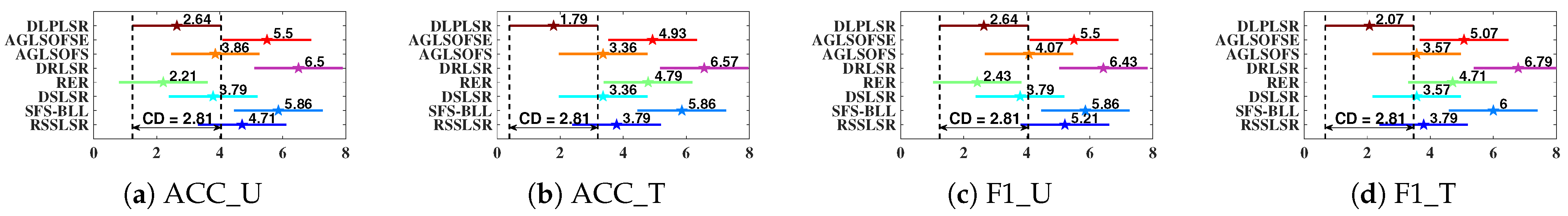
| Average | 4.71 | 5.86 | 3.79 | 2.21 | 6.50 | 3.86 | 5.50 | 2.64 | 3.79 | 5.86 | 3.36 | 4.79 | 6.57 | 3.36 | 4.93 | 1.79 |
| Unlabeled | Testing | |||||||||||||||
|---|---|---|---|---|---|---|---|---|---|---|---|---|---|---|---|---|
| RSSLSR | SFS | DSLSR | RER | DRLSR | AGLSOFS | AGLSOFSE | DLPLSR | RSSLSR | SFS | DSLSR | RER | DRLSR | AGLSOFS_N | AGLSOFS_E | DLPLSR | |
| Iris | 58.33 (8) | 84.28 (6) | 95.48 (1) | 92.35 (3) | 89.61 (4) | 89.09 (5) | 62.19 (7) | 95.48 (1) | 100.00 (1) | 96.17 (6) | 100.00 (1) | 100.00 (1) | 95.92 (7) | 94.59 (8) | 98.62 (5) | 100.00 (1) |
| Wine | 68.76 (5) | 72.78 (4) | 76.14 (3) | 67.43 (6) | 59.63 (7) | 78.82 (2) | 20.29 (8) | 91.64 (1) | 69.45 (6) | 68.99 (7) | 82.87 (3) | 69.82 (5) | 59.51 (8) | 84.81 (1) | 76.23 (4) | 84.42 (2) |
| USPS | 85.55 (6) | 54.57 (8) | 87.92 (3) | 95.21 (1) | 88.61 (2) | 86.36 (5) | 75.34 (7) | 86.61 (4) | 87.06 (2) | 55.13 (8) | 86.90 (3) | 81.32 (7) | 87.09 (1) | 85.04 (5) | 84.60 (6) | 85.40 (4) |
| 2k2k | 73.37 (6) | 75.82 (4) | 75.29 (5) | 86.57 (1) | 64.90 (7) | 78.09 (2) | 64.41 (8) | 77.27 (3) | 78.72 (3) | 76.53 (6) | 77.25 (5) | 73.97 (7) | 64.62 (8) | 79.19 (2) | 77.90 (4) | 79.60 (1) |
| 10k | 80.71 (5) | 80.59 (6) | 83.75 (4) | 93.24 (1) | 78.93 (7) | 84.00 (3) | 69.79 (8) | 84.75 (2) | 83.92 (3) | 80.75 (6) | 83.13 (4) | 78.40 (8) | 79.56 (7) | 85.49 (1) | 82.93 (5) | 84.36 (2) |
| Semeion | 69.02 (5) | 54.57 (7) | 75.93 (4) | 78.74 (2) | 31.39 (8) | 77.92 (3) | 60.28 (6) | 79.13 (1) | 75.67 (4) | 55.13 (7) | 71.06 (5) | 70.21 (6) | 33.98 (8) | 80.92 (1) | 78.21 (3) | 80.05 (2) |
| COIL20 | 76.85 (6) | 80.14 (4) | 82.70 (2) | 85.34 (1) | 59.78 (8) | 78.22 (5) | 66.76 (7) | 81.94 (3) | 79.69 (5) | 79.11 (6) | 83.58 (1) | 79.77 (4) | 61.30 (8) | 77.75 (7) | 81.53 (3) | 83.26 (2) |
| COIL100 | 51.61 (7) | 66.81 (4) | 71.57 (2) | 75.01 (1) | 52.67 (6) | 66.67 (5) | 41.62 (8) | 67.55 (3) | 60.37 (7) | 65.31 (3) | 69.78 (1) | 63.30 (6) | 50.59 (8) | 65.07 (4) | 64.44 (5) | 65.86 (2) |
| ORL | 23.69 (4) | 9.75 (8) | 23.20 (5) | 18.68 (6) | 17.62 (7) | 25.19 (3) | 31.44 (1) | 25.26 (2) | 29.29 (4) | 14.27 (8) | 28.52 (5) | 32.73 (2) | 26.51 (7) | 32.73 (3) | 27.34 (6) | 33.25 (1) |
| Jaffe | 93.56 (4) | 83.08 (7) | 96.75 (2) | 98.23 (1) | 53.05 (8) | 87.25 (6) | 94.53 (3) | 93.49 (5) | 92.48 (3) | 85.98 (7) | 100.00 (1) | 89.13 (5) | 51.40 (8) | 86.81 (6) | 91.40 (4) | 98.12 (2) |
| PIX10 | 12.58 (8) | 22.11 (6) | 22.53 (4) | 32.54 (2) | 20.11 (7) | 22.26 (5) | 79.90 (1) | 24.62 (3) | 37.62 (6) | 39.49 (2) | 37.89 (5) | 37.89 (4) | 35.93 (7) | 39.90 (1) | 34.97 (8) | 39.01 (3) |
| Yale | 20.04 (3) | 19.43 (4) | 16.72 (6) | 21.65 (2) | 10.25 (8) | 15.13 (7) | 38.84 (1) | 18.95 (5) | 21.66 (7) | 24.04 (5) | 29.07 (1) | 27.60 (4) | 8.12 (8) | 27.93 (3) | 22.97 (6) | 28.13 (2) |
| YaleB | 58.10 (4) | 12.39 (8) | 52.52 (5) | 30.79 (6) | 59.79 (3) | 60.21 (2) | 19.33 (7) | 62.52 (1) | 62.50 (1) | 15.05 (8) | 51.12 (7) | 56.99 (5) | 60.98 (3) | 57.58 (4) | 53.81 (6) | 61.23 (2) |
| AR | 30.99 (2) | 14.64 (6) | 0.48 (7) | 51.78 (1) | 0.02 (8) | 22.65 (4) | 14.88 (5) | 23.96 (3) | 32.69 (1) | 13.53 (5) | 0.02 (8) | 24.97 (2) | 0.76 (7) | 21.97 (4) | 11.22 (6) | 23.21 (3) |
| Average | 5.21 | 5.86 | 3.79 | 2.43 | 6.43 | 4.07 | 5.50 | 2.64 | 3.79 | 6 | 3.57 | 4.71 | 6.79 | 3.57 | 5.07 | 2.07 |
| Time | 10k | 2k2k | AR | COIL100 | COIL20 | Iris | Jaffe | ORL | PIX10 | Semeion | USPS | Wine | Yale | YaleB | AveT | AveR |
|---|---|---|---|---|---|---|---|---|---|---|---|---|---|---|---|---|
| RSSLSR | 216.60 (5) | 16.27 (4) | 36.23 (4) | 76.87 (4) | 1.07 (4) | 0.00 (2) | 0.01 (2) | 0.06 (1) | 0.00 (1) | 1.71 (3) | 140.23 (6) | 0.00 (2) | 0.01 (1) | 4.40 (5) | 35.25 (4) | 3.14 (3) |
| SFS_BLL | 552.66 (7) | 292.03 (8) | 324.55 (7) | 942.07 (8) | 8.29 (8) | 0.01 (4) | 0.02 (4) | 0.26 (6) | 0.01 (3) | 7.68 (7) | 7.68 (1) | 0.01 (4) | 0.03 (3) | 31.76 (8) | 154.79 (7) | 5.57 (6) |
| DSLSR | 42.31 (2) | 11.78 (3) | 20.40 (2) | 65.83 (3) | 1.15 (5) | 0.00 (1) | 0.01 (1) | 0.06 (2) | 0.00 (2) | 1.68 (2) | 60.00 (4) | 0.00 (1) | 0.01 (2) | 3.40 (4) | 14.76 (2) | 2.43 (1) |
| RER | 907.55 (8) | 110.90 (7) | 301.14 (6) | 503.40 (7) | 3.91 (7) | 0.02 (7) | 0.05 (7) | 0.21 (5) | 0.02 (5) | 8.50 (8) | 517.86 (8) | 0.03 (6) | 0.04 (5) | 15.56 (7) | 169.23 (8) | 6.64 (8) |
| DRLSR | 229.03 (6) | 23.06 (6) | 9.38 (1) | 97.05 (6) | 0.91 (3) | 0.01 (6) | 0.05 (5) | 0.12 (3) | 0.04 (7) | 2.37 (5) | 166.95 (7) | 0.05 (8) | 0.05 (6) | 2.19 (3) | 37.95 (5) | 5.14 (5) |
| AGLSOFS_N | 125.67 (4) | 21.20 (5) | 415.23 (8) | 81.20 (5) | 2.51 (6) | 0.04 (8) | 0.15 (8) | 0.92 (8) | 0.13 (8) | 3.93 (6) | 63.49 (5) | 0.05 (7) | 0.24 (8) | 9.10 (6) | 51.71 (6) | 6.57 (7) |
| AGLSOFS_E | 44.99 (3) | 4.81 (1) | 24.00 (3) | 26.37 (2) | 0.41 (1) | 0.00 (3) | 0.02 (3) | 0.14 (4) | 0.02 (4) | 0.67 (1) | 59.67 (3) | 0.00 (3) | 0.03 (4) | 1.65 (1) | 11.63 (1) | 2.57(2) |
| DLPLSR | 31.53 (1) | 5.00 (2) | 170.24 (5) | 22.95 (1) | 0.72 (2) | 0.01 (5) | 0.05 (6) | 0.31 (7) | 0.04 (6) | 2.10 (4) | 58.40 (2) | 0.02 (5) | 0.09 (7) | 2.11 (2) | 20.97(3) | 3.93 (4) |
| Datasets | ACC_U | ACC_T | F1_U | F1_T | ||||||||||||
|---|---|---|---|---|---|---|---|---|---|---|---|---|---|---|---|---|
| w | 1 | 2 | 4 | w | 1 | 2 | 4 | w | 1 | 2 | 4 | w | 1 | 2 | 4 | |
| Iris | 95.52 | 95.52 | 95.52 | 95.52 | 100.00 | 100.00 | 100.00 | 100.00 | 95.48 | 95.48 | 95.48 | 95.48 | 100.00 | 100.00 | 100.00 | 100.00 |
| Wine | 91.25 | 90.00 | 91.25 | 68.75 | 84.27 | 82.02 | 82.02 | 73.03 | 91.64 | 90.60 | 91.64 | 67.10 | 84.42 | 82.27 | 82.27 | 71.92 |
| USPS | 87.91 | 87.33 | 87.31 | 88.31 | 86.75 | 86.62 | 86.62 | 86.17 | 86.61 | 86.16 | 86.12 | 87.07 | 85.40 | 85.46 | 85.46 | 84.78 |
| 2k2k | 77.39 | 77.11 | 78.06 | 78.22 | 79.95 | 79.65 | 79.80 | 79.35 | 77.27 | 77.03 | 77.93 | 78.11 | 79.60 | 79.26 | 79.40 | 78.93 |
| 10k | 85.11 | 85.07 | 85.07 | 85.33 | 84.66 | 84.68 | 84.66 | 85.06 | 84.75 | 84.69 | 84.70 | 84.99 | 84.36 | 84.37 | 84.36 | 84.76 |
| Semeion | 79.19 | 77.23 | 78.07 | 77.93 | 80.18 | 80.43 | 78.17 | 80.93 | 79.13 | 77.17 | 77.99 | 77.92 | 80.05 | 80.46 | 78.21 | 80.73 |
| COIL20 | 82.56 | 82.10 | 82.56 | 82.72 | 83.47 | 80.56 | 83.47 | 81.39 | 81.94 | 80.64 | 81.94 | 81.16 | 83.26 | 80.43 | 83.26 | 81.51 |
| COIL100 | 68.77 | 67.41 | 68.33 | 67.38 | 65.92 | 64.81 | 65.58 | 64.83 | 67.55 | 66.28 | 67.02 | 66.19 | 65.86 | 64.80 | 65.65 | 64.86 |
| ORL | 23.89 | 19.44 | 23.89 | 20.00 | 52.00 | 44.00 | 51.00 | 43.50 | 25.26 | 20.94 | 26.34 | 21.86 | 33.25 | 27.60 | 32.49 | 27.32 |
| Jaffe | 93.68 | 88.42 | 91.58 | 90.53 | 98.13 | 92.52 | 97.20 | 91.59 | 93.49 | 88.35 | 91.94 | 90.60 | 98.12 | 92.43 | 97.21 | 91.51 |
| PIX10 | 26.67 | 24.44 | 24.44 | 24.44 | 64.00 | 64.00 | 64.00 | 64.00 | 24.62 | 25.91 | 22.99 | 23.95 | 39.01 | 39.36 | 39.12 | 39.27 |
| Yale | 21.62 | 20.27 | 20.27 | 20.27 | 40.96 | 34.94 | 34.94 | 34.94 | 18.95 | 18.20 | 18.20 | 18.20 | 28.13 | 22.72 | 22.72 | 22.72 |
| YaleB | 62.62 | 59.58 | 59.94 | 24.59 | 60.23 | 56.42 | 58.00 | 22.87 | 62.52 | 59.45 | 60.02 | 25.62 | 61.23 | 57.04 | 58.73 | 24.83 |
| AR | 25.47 | 22.91 | 23.25 | 15.04 | 23.31 | 21.77 | 21.85 | 13.31 | 23.96 | 22.50 | 22.64 | 15.69 | 23.21 | 21.70 | 21.64 | 15.34 |
| CWRU | SEU | Average Rank | |||||||
|---|---|---|---|---|---|---|---|---|---|
| ACC_U | ACC_T | F1_U | F1_T | ACC_U | ACC_T | F1_U | F1_T | ||
| RSSLSR | 95.59 (1) | 95.05 (1) | 95.14 (1) | 95.10 (1) | 79.86 (6) | 83.80 (4) | 80.18 (6) | 83.79 (4) | 3.00 |
| SFS | 80.17 (5) | 78.81 (4) | 78.05 (5) | 78.59 (4) | 81.04 (5) | 82.29 (6) | 81.02 (5) | 82.30 (6) | 5.00 |
| DSLSR | 95.35 (2) | 92.47 (2) | 95.13 (2) | 92.50 (2) | 98.34 (1) | 98.43 (1) | 98.34 (1) | 98.43 (1) | 1.50 |
| RER | 93.27 (3) | 78.11 (5) | 92.24 (3) | 77.94 (5) | 90.22 (3) | 55.26 (7) | 90.25 (3) | 55.28 (7) | 4.50 |
| DRLSR | 9.91 (8) | 10.14 (8) | 1.80 (8) | 1.84 (8) | 20.14 (7) | 20.00 (8) | 6.70 (7) | 6.67 (8) | 7.75 |
| AGLSOFS | 71.73 (6) | 71.35 (6) | 68.58 (6) | 71.37 (6) | 83.09 (4) | 83.54 (5) | 83.18 (4) | 83.57 (5) | 5.25 |
| AGLSOFSE | 42.23 (7) | 71.07 (7) | 31.30 (7) | 70.77 (7) | 20.14 (7) | 92.56 (3) | 6.70 (7) | 92.56 (3) | 6.00 |
| DLPLSR | 92.04 (4) | 92.35 (3) | 90.72 (4) | 92.20 (3) | 93.35 (2) | 94.39 (2) | 93.38 (2) | 94.39 (2) | 2.75 |
Disclaimer/Publisher’s Note: The statements, opinions and data contained in all publications are solely those of the individual author(s) and contributor(s) and not of MDPI and/or the editor(s). MDPI and/or the editor(s) disclaim responsibility for any injury to people or property resulting from any ideas, methods, instructions or products referred to in the content. |
© 2025 by the authors. Licensee MDPI, Basel, Switzerland. This article is an open access article distributed under the terms and conditions of the Creative Commons Attribution (CC BY) license (https://creativecommons.org/licenses/by/4.0/).
Share and Cite
Zhang, S.; Yang, Z.; Shi, Z. DLPLSR: Dual Label Propagation-Driven Least Squares Regression with Feature Selection for Semi-Supervised Learning. Mathematics 2025, 13, 2290. https://doi.org/10.3390/math13142290
Zhang S, Yang Z, Shi Z. DLPLSR: Dual Label Propagation-Driven Least Squares Regression with Feature Selection for Semi-Supervised Learning. Mathematics. 2025; 13(14):2290. https://doi.org/10.3390/math13142290
Chicago/Turabian StyleZhang, Shuanghao, Zhengtong Yang, and Zhaoyin Shi. 2025. "DLPLSR: Dual Label Propagation-Driven Least Squares Regression with Feature Selection for Semi-Supervised Learning" Mathematics 13, no. 14: 2290. https://doi.org/10.3390/math13142290
APA StyleZhang, S., Yang, Z., & Shi, Z. (2025). DLPLSR: Dual Label Propagation-Driven Least Squares Regression with Feature Selection for Semi-Supervised Learning. Mathematics, 13(14), 2290. https://doi.org/10.3390/math13142290