
A Delayed Malware Propagation Model Under a Distributed Patching Mechanism: Stability Analysis


Abstract
1. Introduction
2. Delayed Malware Propagation Model
2.1. A 3D Model
- ()
- Let , , and denote the number of susceptible, infected, and patched internal nodes at time t, respectively.
- ()
- External nodes enter the network at a constant rate . In what follows, is referred to as the inflow rate.
- ()
- Each internal node leaves the network at a constant rate . In what follows, is referred to as the outflow rate.
- ()
- Due to contact with infected nodes, susceptible internal nodes become infected at time t at rate , where , , and are constants. In what follows, is referred to as the infection force, as the infection coefficient, and as the infection delay.
- ()
- Due to contact with patched nodes, infected nodes get patched at time t at rate , where , , and are constants. In what follows, is referred to as the recovery force, as the recovery coefficient, and as the recovery delay.
- ()
- Due to patch failure, each patched node becomes susceptible at a constant rate . In what follows, and is referred to as the failure rate.
- ()
- Let . In what follows is referred to as the maximum delay.
- ()
- Let , denote the initial condition. Here, , , and are non-negative continuous functions.
- ()
- Due to malware propagation, assume , , .
2.2. The Reduced 2D Model
2.3. Basic Properties of the Delayed SIPS Model
2.4. Basic Reproduction Number for the Delayed SIPS Model
3. Malware-Endemic Equilibrium
- (C1)
- .
- (C2)
- .
- (C1)
- .
- (C2)
- .
- (A1)
- Suppose . Then, model (2) admits no patch-endemic malware-endemic equilibrium.
- (A2)
- Suppose . Then, model (2) admits a unique patch-endemic malware-endemic equilibrium, , , .
- (a)
- In the case where , model (2) admits no malware-endemic equilibrium.
- (b)
- In the case where , model (2) admits a unique patch-free malware-endemic equilibrium and admits no patch-endemic malware-endemic equilibrium. This result reveals that if network parameters result in , the distributed patching process is unsustainable.
- (c)
- In the case where , model (2) admits a unique patch-free malware-endemic equilibrium and admits a unique patch-endemic malware-endemic equilibrium. This result reveals that if network parameters result in , the distributed patching process is sustainable.
4. Dynamics of the Malware-Free Equilibrium
4.1. Local Asymptotic Stability
- (A1)
- Suppose . Then, is locally asymptotically stable.
- (A2)
- Suppose . Then, is unstable.
4.2. Global Asymptotic Stability
5. Dynamics of the Patch-Free Malware-Endemic Equilibrium
- (A1)
- Suppose . Then, is locally asymptotically stable.
- (A2)
- Suppose . Then, is unstable.
- (C1)
- .
- (C2)
- .
- (C3)
- .
6. Dynamics of the Patch-Endemic Malware-Endemic Equilibrium
- (C1)
- .
- (C2)
- .
- (C1)
- .
- (C2)
- .
- (C3)
- .
7. Simulation Experiments
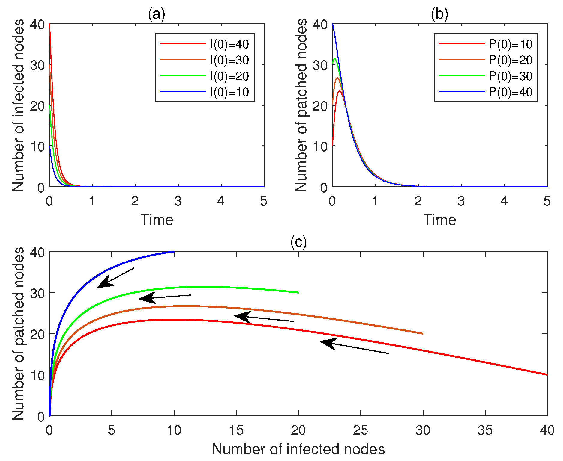
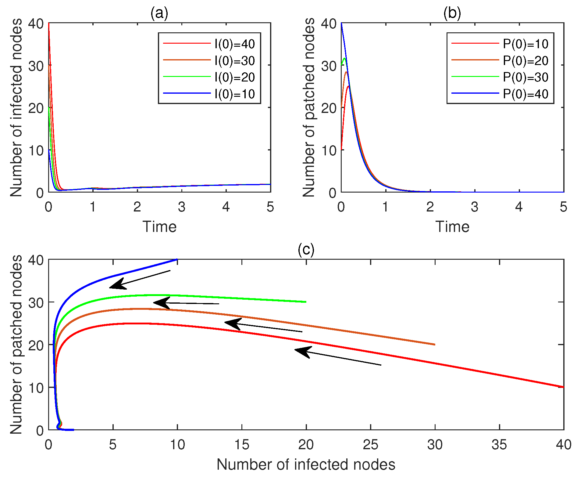
7.1. Asymptotic Stability of the Malware-Free Equilibrium
- (a)
- Let , . Figure 1a,b display and , , respectively. See the red lines.
- (b)
- Let , . Figure 1a,b display and , , respectively. See the brown line.
- (c)
- Let , . Figure 1a,b display and , , respectively. See the green line.
- (d)
- Let , . Figure 1a,b display and , , respectively. See the blue line.
- (e)
- Figure 1c plots the corresponding phase portrait, from which the local asymptotic stability of is observed.
- (a)
- Let , . Figure 2a,b display and , , respectively. See the red lines.
- (b)
- Let , . Figure 2a,b display and , , respectively. See the brown line.
- (c)
- Let , . Figure 2a,b display and , , respectively. See the green line.
- (d)
- Let , . Figure 2a,b display and , , respectively. See the blue line.
- (e)
- Figure 2c plots the corresponding phase portrait, from which the unstability of is observed.
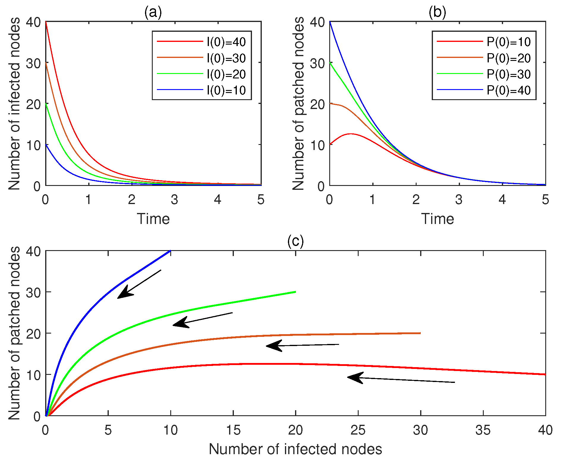
- (a)
- For , let , . Figure 3a,b display and , , respectively. See the red line.
- (b)
- For , let , . Figure 3a,b display and , , respectively. See the brown line.
- (c)
- For , let , . Figure 3a,b display and , , respectively. See the green line.
- (d)
- For , let , . Figure 3a,b display and , , respectively. See the blue line.
- (e)
- Figure 3c plots the corresponding phase portrait, from which the global asymptotic stability of is observed.
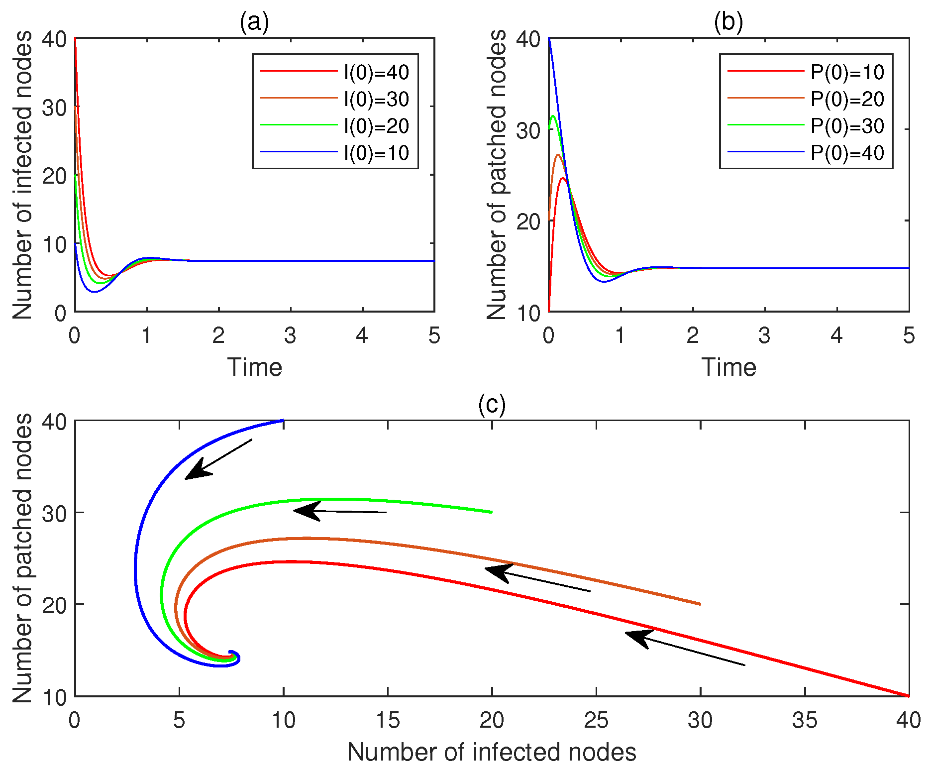
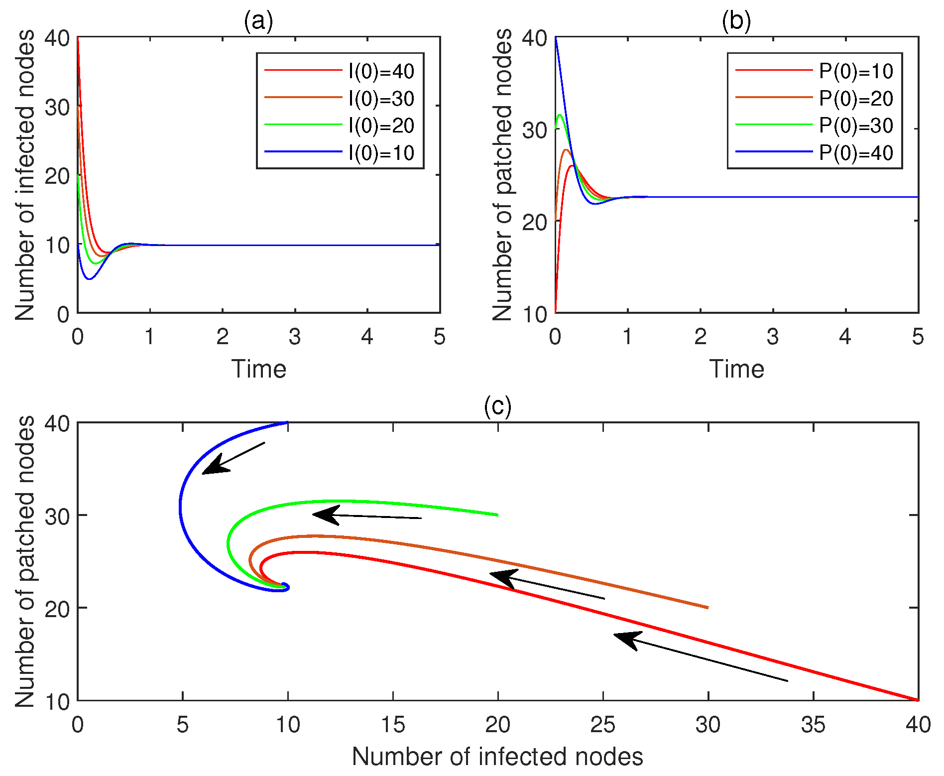
7.2. Asymptotic Stability of the Patch-Free Malware-Endemic Equilibrium
- (a)
- Let , . Figure 4a,b display and , , respectively. See the red lines.
- (b)
- Let , . Figure 4a,b display and , , respectively. See the brown line.
- (c)
- Let , . Figure 4a,b display and , , respectively. See the green line.
- (d)
- Let , . Figure 4a,b display and , , respectively. See the blue line.
- (e)
- Figure 4c plots the corresponding phase portrait, from which the local asymptotic stability of is observed.
- (a)
- Let , . Figure 5a,b display and , , respectively. See the red lines.
- (b)
- Let , . Figure 5a,b display and , , respectively. See the brown line.
- (c)
- Let , . Figure 5a,b display and , , respectively. See the green line.
- (d)
- Let , . Figure 5a,b display and , , respectively. See the blue line.
- (e)
- Figure 5c plots the corresponding phase portrait, from which the unstability of is observed.

- (a)
- For , let , . Figure 6a,b display and , , respectively. See the red line.
- (b)
- For , let , . Figure 6a,b display and , , respectively. See the brown line.
- (c)
- For , let , . Figure 6a,b display and , , respectively. See the green line.
- (d)
- For , let , . Figure 6a,b display and , , respectively. See the blue line.
- (e)
- Figure 6c plots the corresponding phase portrait, from which the local asymptotic stability of is observed.
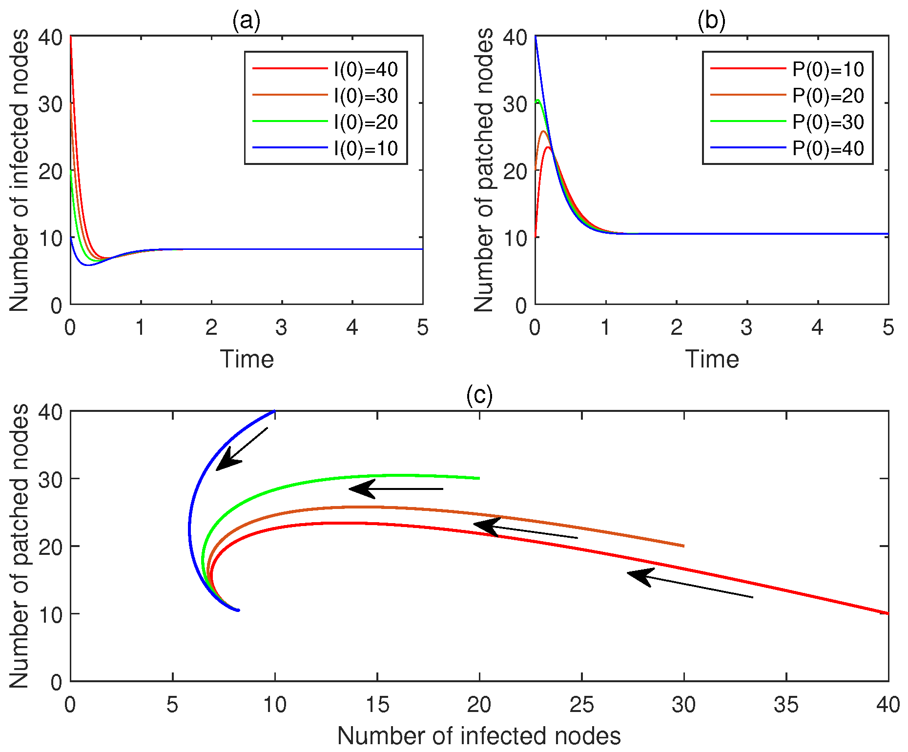
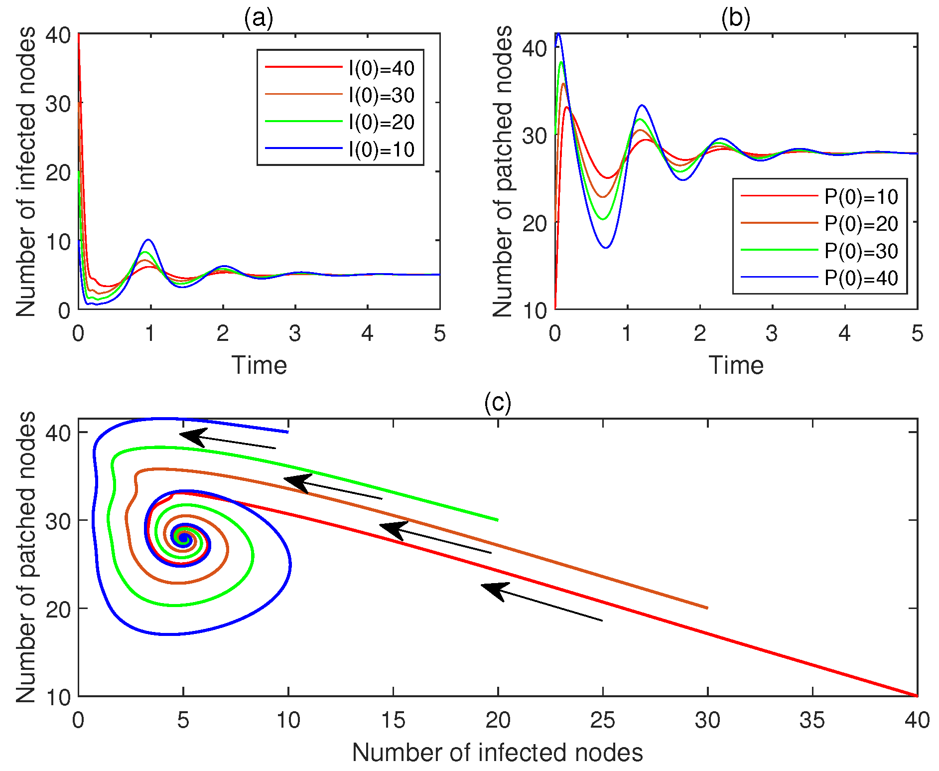
7.3. Asymptotic Stability of the Patch-Endemic Malware-Endemic Equilibrium
- (a)
- Let , . Figure 7a,b display and , , respectively. See the red lines.
- (b)
- Let , . Figure 7a,b display and , , respectively. See the brown line.
- (c)
- Let , . Figure 7a,b display and , , respectively. See the green line.
- (d)
- Let , . Figure 7a,b display and , , respectively. See the blue line.
- (e)
- Figure 7c plots the corresponding phase portrait, from which the local asymptotic stability of is observed.
- (a)
- For , let , . Figure 8a,b display and , , respectively. See the red line.
- (b)
- For , let , . Figure 8a,b display and , , respectively. See the brown line.
- (c)
- For , let , . Figure 8a,b display and , , respectively. See the green line.
- (d)
- For , let , . Figure 8a,b display and , , respectively. See the blue line.
- (e)
- Figure 8c plots the corresponding phase portrait, from which the local asymptotic stability of is observed.
8. Further Discussions
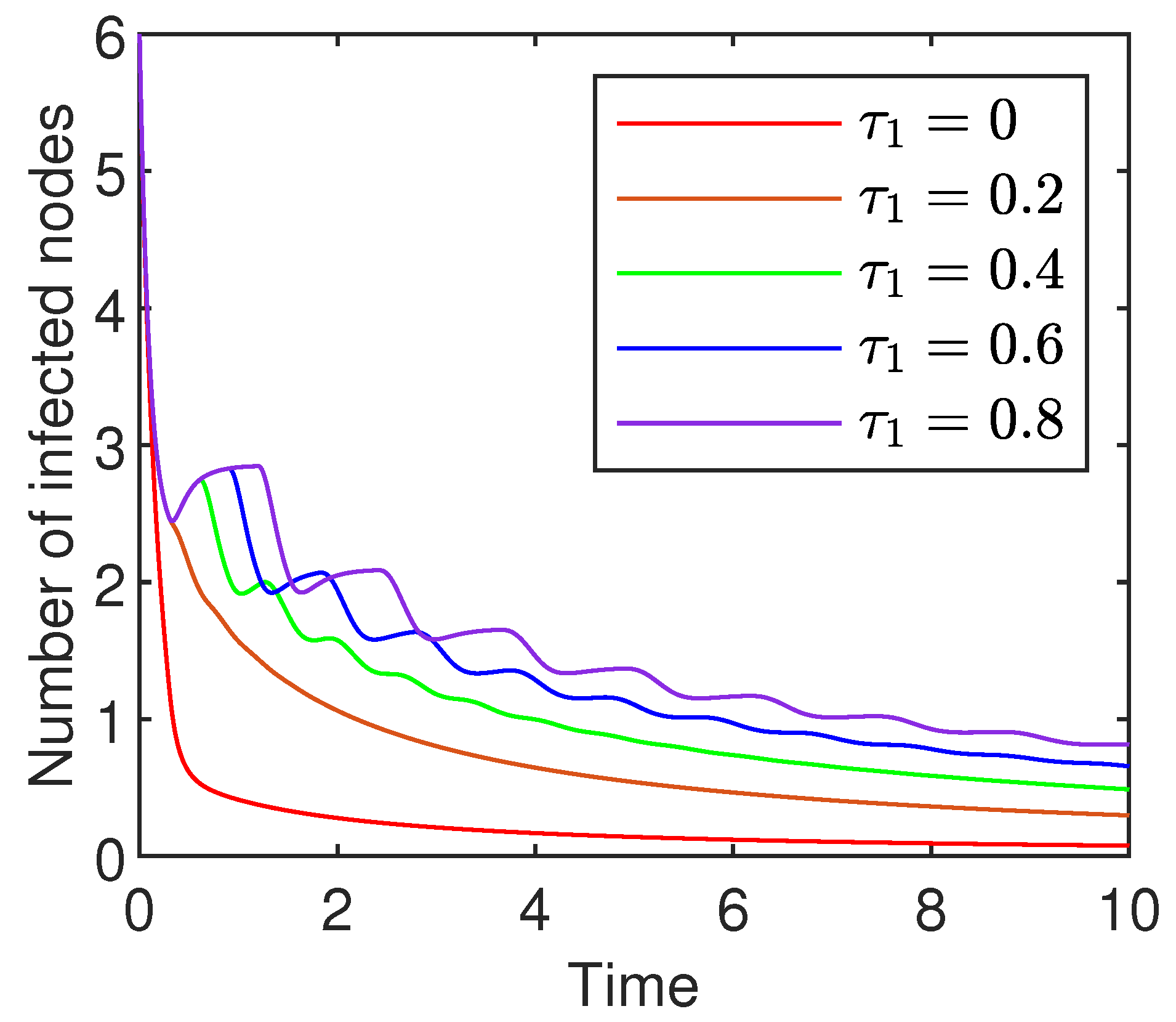
8.1. Influence of the Delays
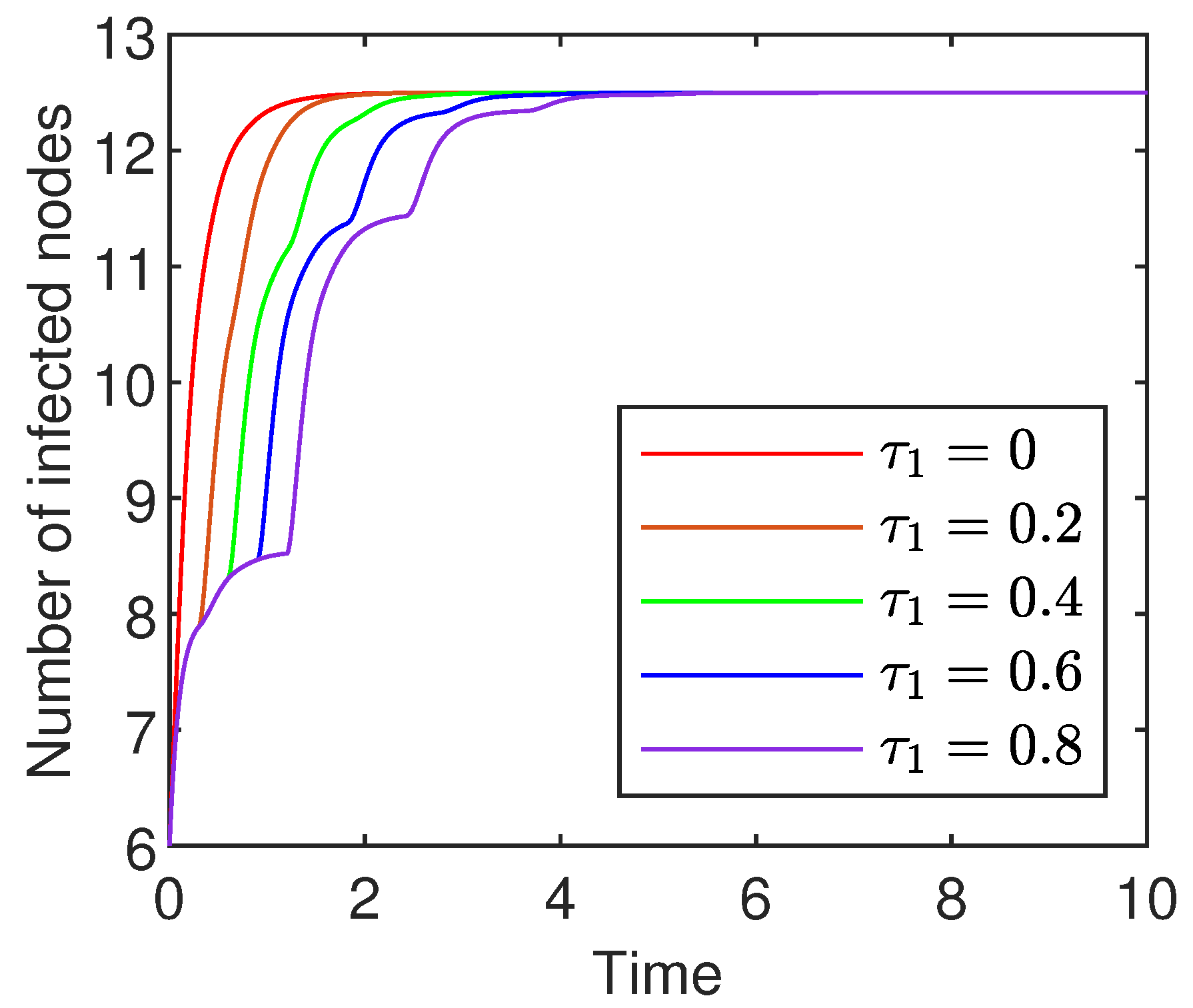
- (a)
- With the extension of the infection delay, the number of infected nodes varies more slowly. This is because the extension leads to a longer time for a susceptible node to become infected and hence slower change in the number of infected nodes.
- (b)
- With the extension of the infection delay, the number of infected nodes oscillates more violently. The delay-induced oscillations suggest that network latency could lead to recurring malware outbreaks even as the system appears to stabilize, posing a challenge for administrators who might prematurely declare an incident is resolved.
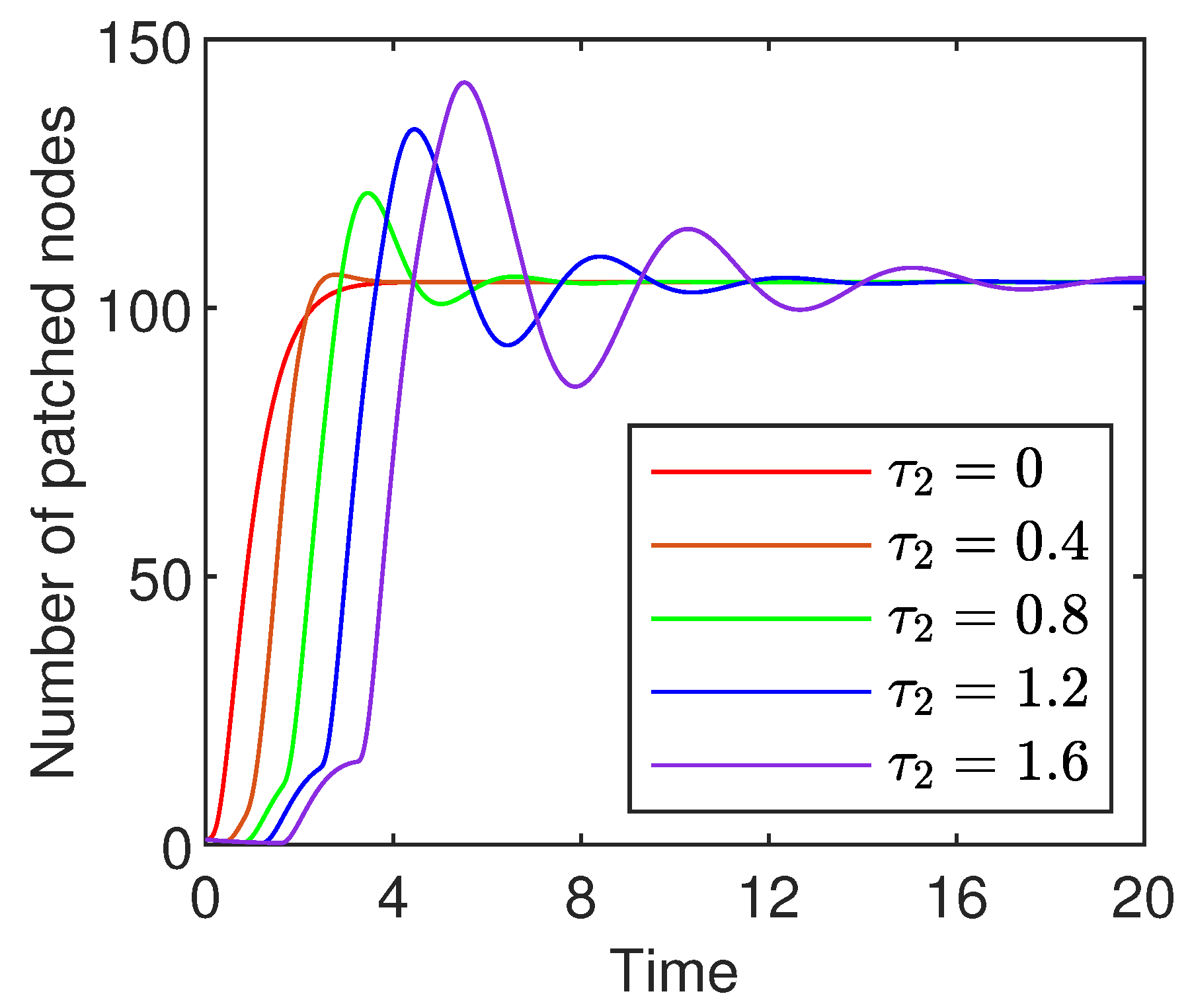
- (a)
- With the extension of the recovery delay, the number of patched nodes varies more slowly. This is because the extension leads to a longer time for an infected node to be patched and hence slower change in the number of patched nodes.
- (b)
- With the extension of the recovery delay, the number of patched nodes oscillates more violently. The delay-induced oscillations suggest that network latency could lead to recurring patch failure even as the system appears to stabilize, posing a challenge for administrators who might prematurely declare a patch dissemination is successful.
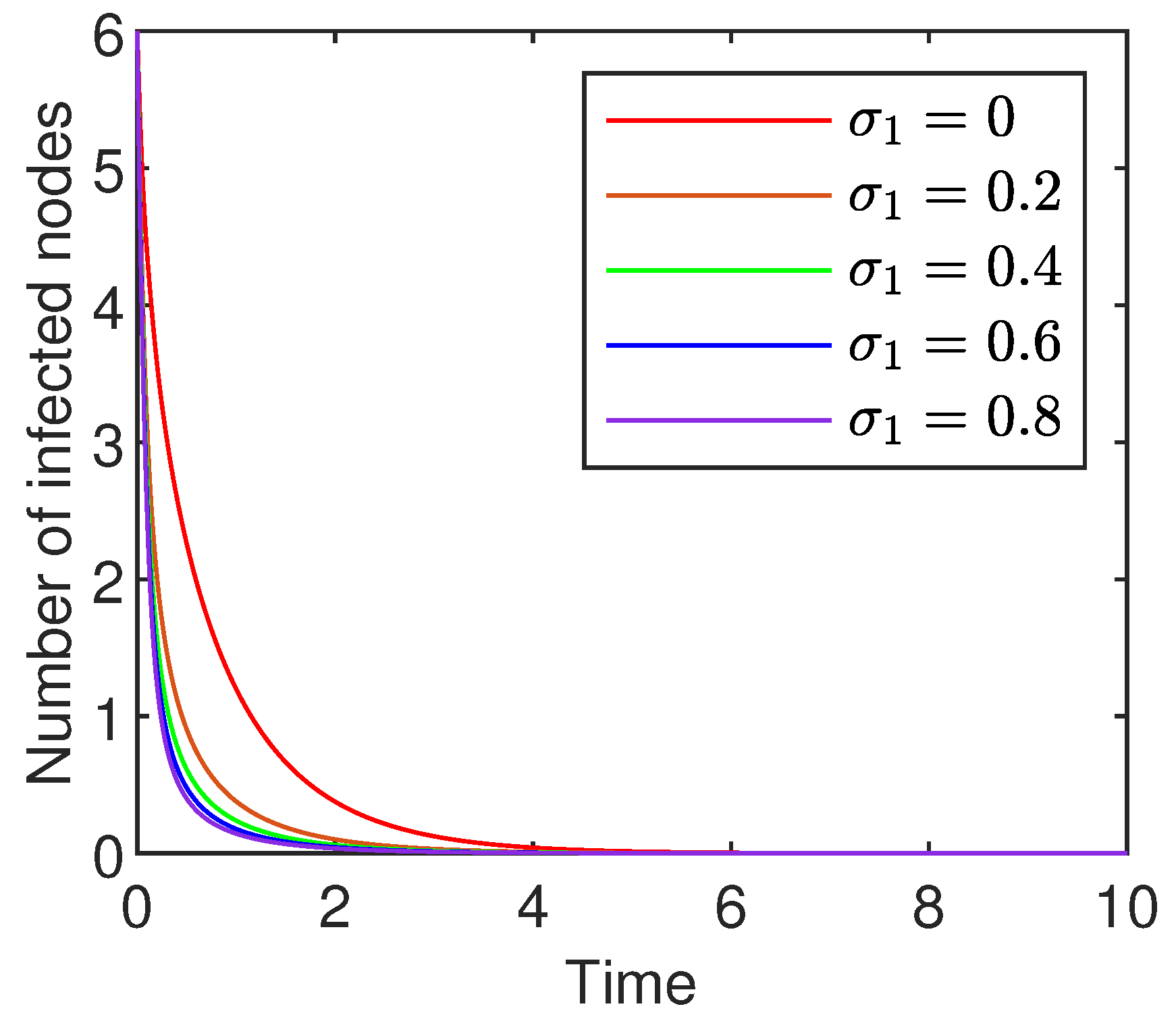
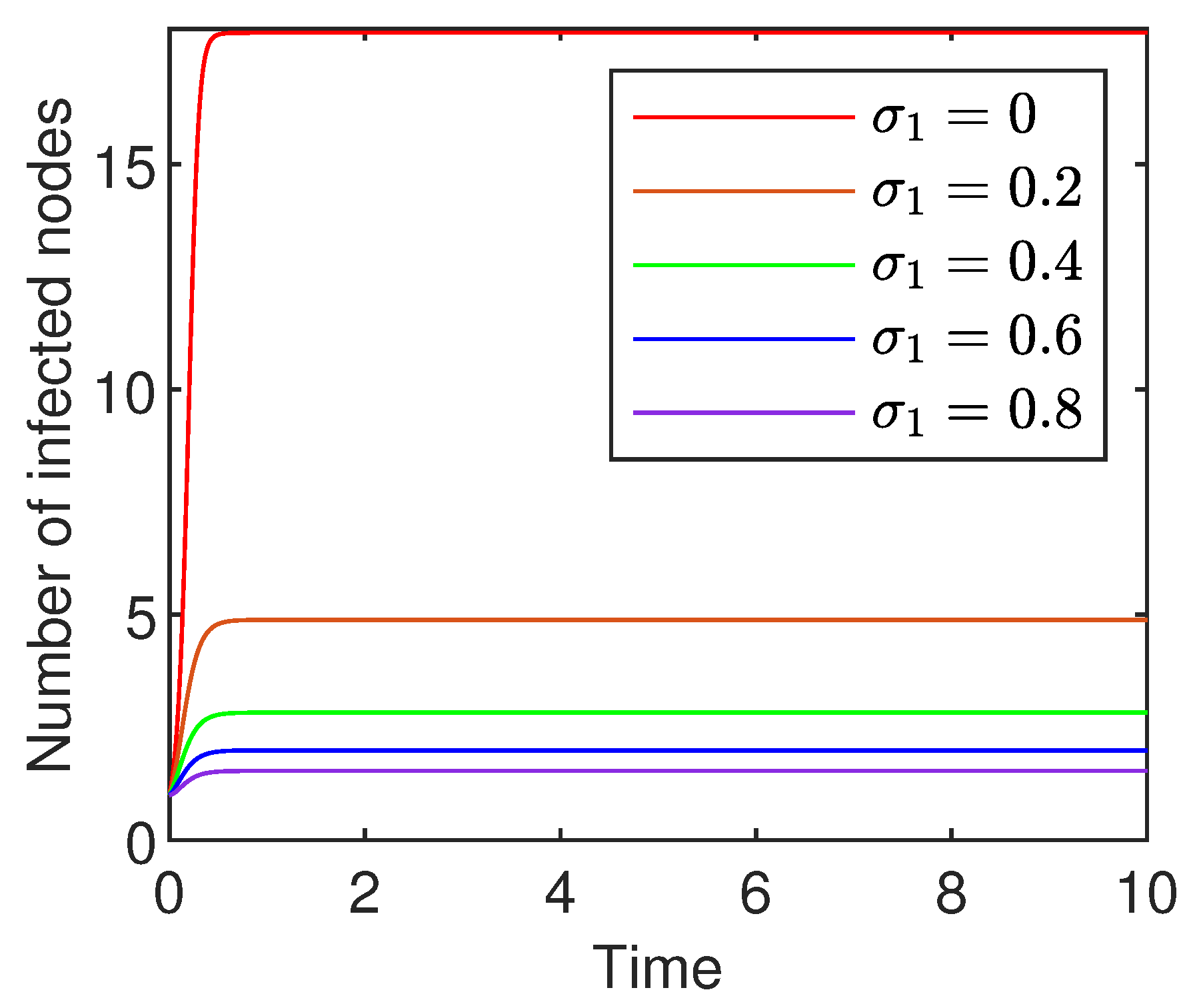
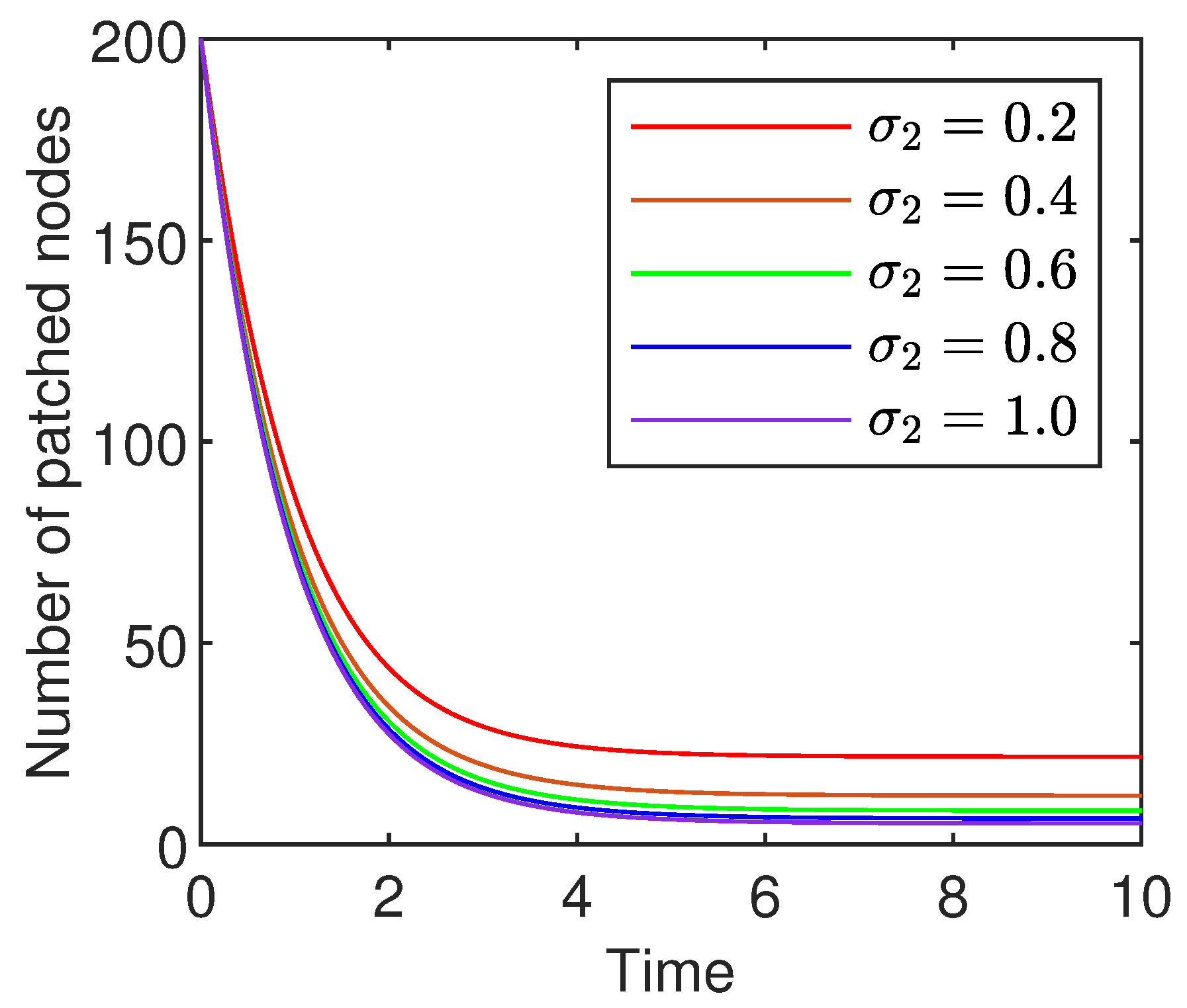
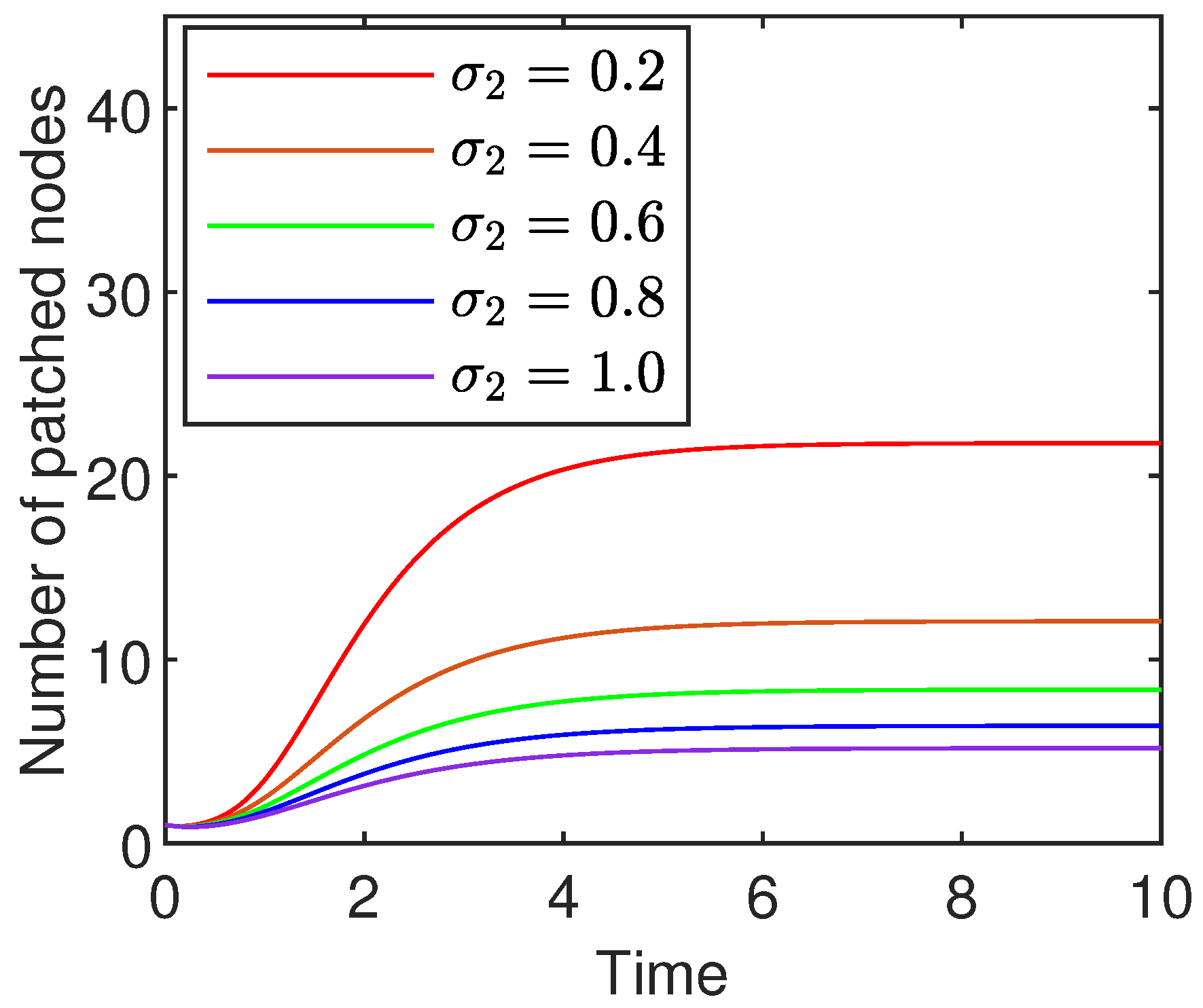
8.2. Influence of the Saturation Coefficients
9. Conclusions
Author Contributions
Funding
Data Availability Statement
Conflicts of Interest
References
- Aycock, J. Computer Viruses and Malware; Springer Science & Business Media: Berlin/Heidelberg, Germany, 2006. [Google Scholar]
- Beaman, C.; Barkworth, A.; Akande, T.D.; Hakak, S.; Khan, M.K. Ransomware: Recent advances, analysis, challenges and future research directions. Comput. Secur. 2021, 111, 102490. [Google Scholar] [CrossRef] [PubMed]
- Admass, W.S.; Munaye, Y.Y. Cyber security: State of the art, challenges and future directions. Cyber Secur. Appl. 2024, 2, 100031. [Google Scholar] [CrossRef]
- Aboaoja, F.A.; Zainal, A.; Ghaleb, F.A.; Al-rimy, B.A.; Eisa, T.A.E.; Elnour, A.A.H. Malware detection issues, challenges, and future directions: A survey. Appl. Sci. 2022, 12, 8482. [Google Scholar] [CrossRef]
- Liu, G.; Fu, C.; Yang, X.; Yang, L.; Feng, Y.; Qin, Y. Study of the antivirus patch testing problem through optimal control modeling. PLoS ONE 2025, 20, e0319916. [Google Scholar] [CrossRef] [PubMed]
- Chen, L.C.; Carley, K.M. The impact of countermeasure propagation on the prevalence of computer viruses. IEEE Trans. Syst. Man Cybern. Part B 2004, 34, 823–833. [Google Scholar] [CrossRef]
- Goldenberg, J.; Shavitt, Y.; Shir, E.; Solomon, S. Distributive immunization of networks against viruses using the ‘honey-pot’ architecture. Nat. Phys. 2005, 1, 184–188. [Google Scholar] [CrossRef]
- Marceau, V.; Noel, P.; Hebert-Dufresne, L.; Allard, A.; Dube, L.J. Modeling the dynamical interaction between epidemics on overlay networks. Phys. Rev. E 2011, 84, 026105. [Google Scholar] [CrossRef]
- Britton, N.F. Essential Mathematical Biology; Springer: Berlin/Heidelberg, Germany, 2003. [Google Scholar]
- Kephart, J.O.; White, S.R. Directed epidemiological models of computer viruses. In Proceedings of the IEEE Computer Society Symposium on Research in Security and Privacy, Los Alamitos, CA, USA, 20–22 May 1991; pp. 343–359. [Google Scholar]
- Kephart, J.O.; White, S.R. Measuring and modeling computer virus prevalence. In Proceedings of the IEEE Computer Society Symposium on Research in Security and Privacy, Los Alamitos, CA, USA, 24–26 May 1993; pp. 2–15. [Google Scholar]
- Piqueira, J.R.C.; Araujo, V.O. A modified epidemiological model for computer viruses. Appl. Math. Comput. 2009, 213, 355–360. [Google Scholar] [CrossRef]
- Toutonji, O.A.; Yoo, S.M.; Park, M. Stability analysis of VEISV propagation modeling for network worm attack. Appl. Math. Model. 2012, 36, 2751–2761. [Google Scholar] [CrossRef]
- Yang, L.X.; Yang, X.; Zhu, Q.; Wen, L. A computer virus model with graded cure rates. Nonlinear Anal. Real World Appl. 2013, 14, 414–422. [Google Scholar] [CrossRef]
- Yang, L.X.; Yang, X. The impact of nonlinear infection rate on the spread of computer virus. Nonlinear Dyn. 2015, 82, 1379–1393. [Google Scholar] [CrossRef]
- Upadhyay, R.K.; Kumari, S.; Misra, A.K. Modeling the virus dynamics in computer network with SVEIR model and nonlinear incident rate. J. Appl. Math. Comput. 2017, 54, 485–509. [Google Scholar] [CrossRef]
- Upadhyay, R.K.; Kumari, S. Bifurcation analysis of an e-epidemic model in wireless sensor. Int. J. Comput. Math. 2018, 95, 1775–1805. [Google Scholar] [CrossRef]
- Zhu, X.; Huang, J.; Qi, C. Modeling and analysis of malware propagation for IoT heterogeneous devices. IEEE Syst. J. 2023, 17, 3846–3857. [Google Scholar] [CrossRef]
- Zhu, Q.; Luo, X.; Liu, Y.; Gan, C.; Wu, Y.; Yang, L.X. Impact of cybersecurity awareness on mobile malware propagation: A dynamical model. Comput. Commun. 2024, 220, 1–11. [Google Scholar] [CrossRef]
- Xiang, H.; Zhang, R.; Wang, Z.; Dong, D. New results on modeling and hybrid control for malware propagation in cyber–physical systems. Comput. Secur. 2025, 157, 104533. [Google Scholar] [CrossRef]
- Quiroga-Sanchez, L.; Montoya, G.A.; Lozano-Garzon, C. The SEIRS-NIMFA epidemiological model for malware propagation analysis in IoT networks. Cybersecurity 2025, 8, 2. [Google Scholar] [CrossRef]
- Yang, L.X.; Yang, X. The effect of infected external computers on the spread of viruses. Phys. A 2013, 392, 6523–6535. [Google Scholar] [CrossRef]
- Yang, L.X.; Yang, X.; Wu, Y. The impact of patch forwarding on the prevalence of computer virus: A theoretical assessment approach. Appl. Math. Model. 2017, 43, 110–125. [Google Scholar] [CrossRef]
- Dong, T.; Liao, X.; Li, H. Stability and Hopf bifurcation in a computer Virus model with multistate antivirus. Abstr. Appl. Anal. 2012, 2012, 841987. [Google Scholar] [CrossRef]
- Yao, Y.; Xie, X.; Guo, H.; Yu, G.; Gao, F.; Tong, X. Hopf bifurcation in an Internet worm propagation model with time delay in quarantine. Math. Comput. Model. 2013, 57, 2635–2646. [Google Scholar] [CrossRef]
- Liu, J. Hopf bifurcation in a delayed SEIQRS model for the transmission of malicious objects in computer network. J. Appl. Math. 2014, 2014, 492198. [Google Scholar] [CrossRef]
- Ren, J.; Xu, Y. Stability and bifurcation of a computer virus propagation model with delay and incomplete antivirus ability. Math. Probl. Eng. 2014, 2014, 475934. [Google Scholar] [CrossRef]
- Yao, Y.; Feng, X.; Yang, W.; Xiao, W.; Gao, F. Analysis of a delayed Internet worm propagation model with impulsive quarantine strategy. Math. Probl. Eng. 2014, 2014, 369360. [Google Scholar] [CrossRef]
- Zhang, Z.; Yang, H. Hopf biburcation of an SIQR computer virus model with time delay. Discret. Dyn. Nat. Soc. 2015, 2015, 101874. [Google Scholar]
- Zhang, Z.; Bi, D. Bifurcation analysis in a delayed computer virus model with the effect of external computers. Adv. Differ. Equ. 2015, 2015, 317. [Google Scholar] [CrossRef]
- Li, C.; Liao, X. The impact of hybrid quarantine strategies and delay factor on viral prevalence in computer networks. Math. Model. Nat. Phenom. 2016, 11, 105–119. [Google Scholar] [CrossRef]
- Zhao, T.; Zhang, Z.; Upadhyay, R.K. Delay-induced Hopf bifurcation of an SVEIR computer virus model with nonlinear incidence rate. Adv. Differ. Equ. 2018, 2018, 256. [Google Scholar] [CrossRef]
- Zhang, Z.; Ranjit Kumar Upadhyay, R.R.; Bi, D.; Wei, R. Stability and Hopf bifurcation of a delayed epidemic model of computer virus with impact of antivirus software. Discret. Dyn. Nat. Soc. 2018, 2018, 8239823. [Google Scholar] [CrossRef]
- Yao, Y.; Fu, Q.; Yang, W.; Wang, Y.; Sheng, C. An epidemic model of computer worms with time delay and variable infection rate. Secur. Commun. Netw. 2018, 2018, 9756982. [Google Scholar] [CrossRef]
- Zhang, Z.; Kundu, S.; Wei, R. A delayed epidemic model for propagation of malicious codes in wireless sensor network. Mathematics 2019, 7, 396. [Google Scholar] [CrossRef]
- Zhang, Z.; Kumari, S.; Upadhyay, R.K. A delayed e-epidemic SLBS model for computer virus. Adv. Differ. Equ. 2019, 2019, 414. [Google Scholar] [CrossRef]
- MadhuSudanan, V.; Geetha, R. Dynamics of epidemic computer virus spreading model with delays. Wirel. Pers. Commun. 2020, 115, 2047–2061. [Google Scholar] [CrossRef]
- Zhang, W.; Wang, Z.; Zhang, Z.; Zou, J. Delay effect on a malware propagation model incorporating user awareness. In Proceedings of the 2022 International Conference on Cyber-Physical Social Intelligence (ICCSI), Nanjing, China, 18–21 November 2022; pp. 555–560. [Google Scholar]
- Yu, X.; Zeb, A.; Zhang, Z. Mathematical analysis of a delayed malware propagation model on mobile wireless sensor network. Fractals 2022, 30, 2240160. [Google Scholar] [CrossRef]
- Liu, J.; Saeed, I.; Zeb, A. Delay effect of an e-epidemic SEIRS malware propagation model with a generalized non-monotone incidence rate. Results Phys. 2022, 39, 105672. [Google Scholar] [CrossRef]
- Ding, J.; Gul, N.; Liu, G.; Saeed, T. Dynamical aspects of a delayed computer viruses model with horizontal and vertical dissemination over internet. Fractals 2023, 31, 2340092. [Google Scholar] [CrossRef]
- Zhang, Z.; Madhusudanan, V.; Murthy, B.S.N. Effect of delay in SMS worm propagation in mobile network with saturated incidence rate. Wirel. Pers. Commun. 2023, 131, 659–678. [Google Scholar] [CrossRef]
- Wu, G.; Zhang, Y.; Zhang, H.; Yu, S.; Yu, S.; Shen, S. SIHQR model with time delay for worm spread analysis in IIoT-enabled PLC network. Ad Hoc Netw. 2024, 160, 103504. [Google Scholar] [CrossRef]
- Nithya, D.; Madhusudanan, V.; Murthy, B.S.N.; Geetha, R.; Mung, N.X.; Dao, N.; Cho, S. Delayed dynamics analysis of SEI2RS malware propagation models in cyber–Physical systems. Comput. Netw. 2024, 248, 110481. [Google Scholar] [CrossRef]
- Ren, J.; Yang, X.; Yang, L.; Xu, Y.; Yang, F. A delayed computer virus propagation and its dynamics. Chaos Solitons Fractals 2012, 45, 74–79. [Google Scholar] [CrossRef]
- Feng, L.; Liao, X.; Han, Q. Hopf bifurcation analysis of a delayed viral infection model in computer networks. Math. Comput. Model. 2012, 56, 167–179. [Google Scholar] [CrossRef]
- Muroya, Y.; Enatsu, Y.; Li, H. Global stability of a delayed SIRS computer virus propagation model. Int. J. Comput. Math. 2013, 6, 1350001. [Google Scholar] [CrossRef]
- Zhang, Z.; Yang, H. Hopf bifurcation analysis for a computer virus model with two delays. Abstr. Appl. Anal. 2013, 2013, 560804. [Google Scholar] [CrossRef]
- Zhang, Z.; Yang, H. Stability and Hopf bifurcation in a delayed SEIRS worm model in computer network. Math. Probl. Eng. 2013, 2013, 319174. [Google Scholar] [CrossRef]
- Liu, J.; Bianca, C.; Guerrini, L. Dynamical analysis of a computer virus model with delays. Discret. Dyn. Nat. Soc. 2016, 2016, 5649584. [Google Scholar] [CrossRef]
- Zhao, T.; Bi, D. Hopf bifurcation of a computer virus spreading model in the network with limited anti-virus ability. Adv. Differ. Equ. 2017, 2017, 183. [Google Scholar] [CrossRef]
- Zhao, T.; Wei, S.; Bi, D. Hopf bifurcation of a computer virus propagation model with two delays and infectivity in latent period. Syst. Sci. Control Eng. 2018, 6, 90–101. [Google Scholar] [CrossRef]
- Chu, Y.; Xia, W.; Wang, Z. A delayed computer virus model with nonlinear incidence rate. Syst. Sci. Control. Eng. Open Access J. 2019, 7, 389–406. [Google Scholar] [CrossRef]
- Han, X.; Tan, Q. Dynamical behavior of computer virus on Internet. Appl. Math. Comput. 2020, 217, 2520–2526. [Google Scholar] [CrossRef]
- Yang, W.; Fu, Q.; Yao, Y. A malware propagation model with dual delay in the industrial control network. Complexity 2023, 2023, 8823080. [Google Scholar] [CrossRef]
- Yu, X.; Zhang, Z. A delayed malware propagation model for cloud computing security. Fractals 2024, 2024, 2540064. [Google Scholar] [CrossRef]
- Sangala, A.; Hazarika, A.; Neelisetti, R.K.; Basu, R. Analyzing computer virus propagation: Integrating Monte Carlo simulations with delay differential equation models. In Proceedings of the 2024 International Conference on Emerging Techniques in Computational Intelligence (ICETCI), Hyderabad, India, 22–24 August 2024; pp. 345–352. [Google Scholar]
- Nilam, K.G. Stability behavior of a nonlinear mathematical epidemic transmission model with time delay. Nonlinear Dyn. 2019, 98, 1501–1518. [Google Scholar]
- Nilam, K.G. A mathematical and numerical study of a SIR epidemic model with time delay, nonlinear incidence and treatment rates. Theory Biosci. 2019, 138, 203–213. [Google Scholar]
- Nilam, A.K. Mathematical analysis of a delayed epidemic model with nonlinear incidence and treatment rates. J. Eng. Math. 2019, 115, 1–20. [Google Scholar]
- Nilam, A.K. Effects of nonmonotonic functional responses on a disease transmission model: Modeling and simulation. Commun. Math. Stat. 2022, 195, 214. [Google Scholar]
- Avila-Vales, E.; Perez, A.G.C. Dynamics of a time-delayed SIR epidemic model with logistic growth and saturated treatment. Chaos Solitons Fractals 2019, 127, 55–69. [Google Scholar] [CrossRef]
- Nilam, A.K. Stability of a delayed SIR epidemic model by introducing two explicit treatment classes along with nonlinear incidence rate and holling type treatment. Comput. Appl. Math. 2019, 38, 130. [Google Scholar]
- Goel, K.; Nilam, A.K. A deterministic time-delayed SVIRS epidemic model with incidences and saturated treatment. J. Eng. Math. 2020, 121, 19–38. [Google Scholar] [CrossRef]
- Sheng, T.; Fu, C.; Yang, X.; Qin, Y.; Yang, L. Asymptotic stability of a rumor spreading model with three time delays and two saturation functions. Mathematics 2025, 13, 2015. [Google Scholar] [CrossRef]
- Xiao, D.; Ruan, S. Global analysis of an epidemic model with nonmonotone incidence rate. Math. Biosci. 2007, 208, 419–429. [Google Scholar] [CrossRef]
- Buonomo, B.; Rionero, S. On the Lyapunov stability for SIRS epidemic models with general nonlinear incidence rate. Appl. Math. Comput. 2010, 217, 4010–4016. [Google Scholar] [CrossRef]
- Hale, J. Theory of Functional Differential Equations. Springer: New York, NY, USA, 1977. [Google Scholar]
- Diekmann, O.; Heesterbeek, J.A.P.; Metz, J.A.J. On the definition and the computation of the basic reproduction ratio R0 in models for infectious diseases in heterogeneous populations. J. Math. Biol. 1990, 28, 365–382. [Google Scholar] [CrossRef] [PubMed]
- Van den Driessche, P.; Watmough, J. Reproduction numbers and sub-threshold endemic equilibria for compartmental models of disease transmission. Math. Biosci. 2002, 180, 29–48. [Google Scholar] [CrossRef] [PubMed]
- Wei, H.; Li, X.; Martcheva, M. An epidemic model of a vector-borne disease with direct transmission and time delay. J. Math. Anal. Appl. 2008, 342, 895–908. [Google Scholar] [CrossRef]
- Ruan, S.; Wei, J. On the zeros of transcendental functions with applications to stability of delay differential equations with two delays. Dyn. Contin. Discret. Impuls. Syst. 2003, 10, 863–874. [Google Scholar]
- Robinson, R.K. An Introduction to Dynamical Systems: Continuous and Discrete, 2nd ed.; Amer Mathematical Society: Providence, RI, USA, 2012. [Google Scholar]
- Zhu, L.; Zhao, H.; Wang, X. Stability and bifurcation analysis in a delayed reaction-diffusion malware propagation model. Comput. Math. Appl. 2015, 69, 852–887. [Google Scholar] [CrossRef]
- Zhu, L.; Zhao, H.; Wang, X. Bifurcation analysis of a delay reaction-diffusion malware propagation model with feedback control. Commun. Nonlinear Sci. Numer. Simul. 2015, 22, 747–768. [Google Scholar] [CrossRef]
- Du, B.; Wang, H. Partial differential equation modeling of malware propagation in social networks with mixed delays. Comput. Math. Appl. 2018, 75, 3537–3548. [Google Scholar] [CrossRef]
- Balachandran, K. An Introduction to Fractional Differential Equations; Springer: Berlin/Heidelberg, Germany, 2023. [Google Scholar]
- Zhou, Y.; Liu, B.; Zhou, K.; Shen, S. Malware propagation model of fractional order, optimal control strategy and simulations. Front. Phys. 2023, 11, 1201053. [Google Scholar] [CrossRef]
- Yang, L.; Song, Q.; Liu, Y. Dynamics analysis of a new fractional-order SVEIR-KS model for computer virus propagation: Stability and Hopf bifurcation. Fractals 2024, 598, 128075. [Google Scholar] [CrossRef]
- Shi, X.; Luo, A.; Chen, X.; Huang, Y.; Huang, C.; Yin, X. The dynamical behaviors of a fractional-order malware propagation model in information networks. Mathematics 2024, 12, 3814. [Google Scholar] [CrossRef]
- Razi, N.; Bano, A.; Ishtiaq, U.; Kamran, T.; Garayev, M.; Popa, I. Probing malware propagation model with variable infection rates under integer, fractional, and fractal–fractional orders. Fractal Fract. 2025, 9, 90. [Google Scholar] [CrossRef]
- Jafar, M.T.; Yang, L.X.; Li, G.; Zhu, Q.; Gan, C. Minimizing malware propagation in Internet of Things networks: An optimal control using feedback loop approach. IEEE Trans. Inf. Forensics Secur. 2024, 19, 9682–9697. [Google Scholar] [CrossRef]
- Cheng, X.; Yang, L.; Zhu, Q.; Gan, C.; Yang, X.; Li, G. Cost-effective hybrid control strategies for dynamical propaganda war game. IEEE Trans. Inf. Forensics Secur. 2024, 19, 9789–9802. [Google Scholar] [CrossRef]
- Anwar, N.; Saddiq, A.; Raja, M.A.R.; Ahmad, I.; Shoaib, M.; Kiani, A.K. Novel machine intelligent expedition with adaptive autoregressive exogenous neural structure for nonlinear multi-delay differential systems in computer virus propagation. Eng. Appl. Artif. Intell. 2025, 146, 110234. [Google Scholar] [CrossRef]

Disclaimer/Publisher’s Note: The statements, opinions and data contained in all publications are solely those of the individual author(s) and contributor(s) and not of MDPI and/or the editor(s). MDPI and/or the editor(s) disclaim responsibility for any injury to people or property resulting from any ideas, methods, instructions or products referred to in the content. |
© 2025 by the authors. Licensee MDPI, Basel, Switzerland. This article is an open access article distributed under the terms and conditions of the Creative Commons Attribution (CC BY) license (https://creativecommons.org/licenses/by/4.0/).
Share and Cite
Zhang, W.; Yang, X.; Yang, L. A Delayed Malware Propagation Model Under a Distributed Patching Mechanism: Stability Analysis. Mathematics 2025, 13, 2266. https://doi.org/10.3390/math13142266
Zhang W, Yang X, Yang L. A Delayed Malware Propagation Model Under a Distributed Patching Mechanism: Stability Analysis. Mathematics. 2025; 13(14):2266. https://doi.org/10.3390/math13142266
Chicago/Turabian StyleZhang, Wei, Xiaofan Yang, and Luxing Yang. 2025. "A Delayed Malware Propagation Model Under a Distributed Patching Mechanism: Stability Analysis" Mathematics 13, no. 14: 2266. https://doi.org/10.3390/math13142266
APA StyleZhang, W., Yang, X., & Yang, L. (2025). A Delayed Malware Propagation Model Under a Distributed Patching Mechanism: Stability Analysis. Mathematics, 13(14), 2266. https://doi.org/10.3390/math13142266