Abstract
The geometric process is a significant monotonic stochastic process widely used in the fields of applied probability, particularly in the failure analysis of repairable systems. For repairable systems modeled by a geometric process, accurate estimation of model parameters is essential. The inference problem for geometric processes has been well-studied in the case of single-sample data. However, multi-sample data may arise when the repair processes of multiple systems are observed simultaneously. This study addresses the non-parametric inference problem for geometric processes based on multi-sample data. Several non-parametric estimators are proposed using the linear regression method, and their asymptotic properties are established. In addition, test statistics are introduced to assess sample homogeneity and to evaluate the significance of the trend observed in the process. The performance of the proposed estimators is evaluated through a comprehensive simulation study under small-sample settings. An artificial data analysis is conducted to model the repair processes of multiple repairable systems using the geometric process. Furthermore, a real-world dataset consisting of multi-sample failure data from two shared memory processors of the Blue Mountain supercomputer is analyzed to demonstrate the practical applicability of the method in multi-sample failure data analysis.
MSC:
62G05; 62G20
1. Introduction
In statistical modeling of datasets that include inter-arrival times of consecutive random events, a common approach is to use counting process models. When the data shows no trend, the homogeneous Poisson process (HPP) or its generalization, the renewal process (RP), may be applied. If the data exhibits a trend, the non-homogeneous Poisson process (NHPP) is often preferred. Two key NHPP models are the Cox––Lewis (log-linear) process and the Weibull (power–law) process. These models are typically used when the data demonstrates a monotonic trend, as their intensity functions are monotonic. For more details on NHPPs, refer to Ascher and Feingold [1] and Cox and Lewis [2]. However, Lam [3] introduced an alternative counting process, the geometric process (GP), to directly model the monotonic trend in the data. Before formally defining the GP, it is essential to revisit the concept of stochastic monotonicity.
Let be the inter-arrival times of a counting process. The process is said to be stochastically increasing (decreasing), if for all and . As a simple example of a monotone stochastic process, the GP is defined as follows. Let be non-negative random variables representing the inter-arrival times of a counting process. Then, the process is said to be a GP with trend parameter if the random variables are independent and identically distributed (iid) with a common distribution function ; see Lam [3]. Clearly, a GP is stochastically increasing when , and stochastically decreasing when . Furthermore, the GP reduces to an RP when . Thus, the GP generalizes the RP while incorporating stochastic monotonicity.
Since its introduction, the GP has been widely used as a suitable model across various fields of applied probability. In particular, it has been applied to model the repair processes of repairable systems. In such systems, it is reasonable to assume that the successive operating times tend to decrease, while the successive repair times tend to increase due to aging effects and accumulated wear. These monotonic patterns make the GP an appropriate model for analyzing such systems. The GP has been extensively studied in the context of reliability, maintainability, failure, and warranty analysis. For instance, Lam [4,5] utilized the GP to determine the optimal replacement policy for repairable systems. Lam and Zhang [6] applied the GP model to analyze a two-component series system with a single repairman. Lam [7], Tang and Lam [8], and Lam and Zhang [9] explored the GP in the context of maintenance analysis for various deteriorating systems. For other recent applications of the GP, see Chan et al. [10,11,12], Wan and Chan [13], Zhang and Wang [14], and Arnold et al. [15]. Notable contributions have also been made by Aydoğdu and Altındağ [16], Pekalp et al. [17], Pekalp and Aydoğdu [18,19,20], and Rasay et al. [21].
For a repairable system modeled by a GP, estimating the expected operating time after each repair is crucial. Let denote the successive operating times after each repair. Assume that the successive operating times follow a GP with trend parameter , so that the process is a GP. Then, the expected operating time and variance are given by , for , where and . Thus, the expected operating time of a repairable system after a given number of repairs depends on the parameters , and . Accurate statistical estimation of these parameters is critical. The inference problem for , and has been thoroughly studied in the literature. Lam [22] proposed some non-parametric estimators using the linear regression method. Parametric estimation approaches have also been developed by Lam and Chan [23], Aydoğdu et al. [24], Chan et al. [25], Kara et al. [26], assuming that follows common failure distributions such as lognormal, gamma, and Weibull. Additional contributions to statistical inference on GP parameters include the works of Biçer et al. [27], Biçer et al. [28], Lone et al. [29], Usta [30], and Yılmaz [31]. Notably, all existing studies regarding the statistical inference of the parameters , and have been based on single-sample data. However, in practical applications, multi-sample data may be required or may naturally arise over multiple repairable units. This can be explained as follows: A repairable system initially begins to function and is repaired when a failure occurs. After the repair, it returns to the functioning state and is repaired again if another failure occurs. This repair process is repeated until the system becomes ineffective. Most systems tend to become inefficient after only a few repairs due to increased repair times and decreased operating times. Once the system becomes ineffective, it should be replaced with a new one. In such cases, only a few successive operating times are observed. These few observations are often insufficient for reliable statistical inference. To address this limitation and obtain enough observations, the repair processes of multiple identical systems should be observed simultaneously. Such observations constitute multi-sample data. Several studies have addressed the statistical analysis of multi-sample data for modeling the failure/repair processes of multiple repairable systems. For example, Garmabaki et al. [32,33] studied the statistical modeling of multiple repairable systems using RP, HPP, or NHPP as alternative repair process models. Na and Chang [34] analyzed multi-sample failure data from multiple repairable systems using an NHPP model, applying it to the Korean National Army tank failure data. Wang et al. [35] analyzed multi-sample data from multiple repairable systems using a specific NHPP model. In these studies, the authors utilized NHPP models with monotonic intensity functions to analyze multi-sample data collected from the repair processes of multiple repairable systems. The GP model should also be considered as an alternative for analyzing multi-sample failure data due to its straightforward implementation for processes exhibiting a monotonic trend. Recently, Altındağ [36] evaluated the statistical analysis of multi-sample GPs with exponential failure times and demonstrated its application in modeling multiple repairable systems. In certain cases, especially when the samples include only a few observations, the assumption of parametric distribution for failure times may be inappropriate. To address this limitation, we investigate the non-parametric inference problem of GPs for multi-sample data and explore its application in modeling failure data from multiple repairable systems.
The remainder of the paper is organized as follows: Section 2 introduces the concept of multi-sample GPs, proposes several non-parametric estimators, and investigates their theoretical properties. It also presents test statistics to assess sample homogeneity and the significance of monotonic trends. Section 3 provides a comprehensive simulation study to evaluate and compare the performance of the proposed estimators. Section 4 presents illustrative examples based on both simulated and real data analyses. Finally, Section 5 summarizes the conclusions.
2. Inference for Multi-Sample of GPs
2.1. Multi-Sample of GPs
Let be a GP with trend parameter . Denote the mean and variance of the random variable by and , respectively. Then, for , it follows that , . To statistically estimate the parameters , , and , a realization of the process must be observed. Let denote the first inter-arrival times of the GP . Then the sample is considered a single realization. If is not sufficiently large, statistical inference for the parameters , and may be unreliable. To overcome this limitation and improve estimation efficiency, multiple realizations of the process should be observed. Let , denote homogeneous GPs sharing a common trend parameter Suppose that for each , a realization of size is observed. If all these GPs are identical, so that they have the same trend parameter and their initial variables are iid with and for all , then the collection is referred to as a multi-sample of the GP .
A multi-sample from a GP can be illustrated in the context of repair processes for repairable systems. Consider identical repairable systems operating simultaneously, where each system undergoes immediate repair upon failure. It is commonly observed that the successive operating times of such systems tend to decrease after each repair. As a result, the sequence of operating times for each system can be suitably modeled by a GP. Assuming that all repair processes are homogeneous across all systems, the combined dataset of operating times from the systems constitutes a multi-sample from a GP. This data structure, observed throughout the repair processes of the identical systems, is illustrated in Figure 1.
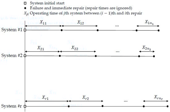
Figure 1.
Repair processes of identical repairable systems.
2.2. Non-Parametric Inference
Let be a multi-sample from independent GPs with a common trend parameter . Assume that all processes are homogeneous; that is, the random variables are iid with , and for . To make inferences about the parameters , , and , we first remind the non-parametric estimation approach based on single-sample data, as proposed by Lam [22] and Lam et al. [37]. Let represent independent samples from a GP with a trend parameter , for . The parameters , , and can be estimated separately from each sample as follows. Define . By the definition of the GP, the random variables for and , are iid. Let us take the logarithm of each . The transformed random variables for and are also iid. Denote the mean and variance of as and for and . By taking the logarithm of the random variable , we obtain for each that
Let us write for each that
where ’s are iid with mean 0 and variance . Rearranging Equation (1) yields for each that
Therefore, Equation (3) can be interpreted as a simple linear regression model for each . By utilizing the least squares method, the least squares estimators of , , and based on the th sample are obtained as follows:
Hence, the least squares estimator of for the th sample is given by . For the details, see Lam [22]. Additionally, Lam [22] proposed several non-parametric estimators for the parameters and as follows. Let us consider Equations (1) and (2). Lam [22] showed that
Thus, the parameter can be estimated from the th sample as:
Alternatively, as suggested by Lam [22], define , for and . Then, a modified moment estimator for , based on the th sample, as defined as:
where . Furthermore, it can be written for each that:
where and ; see Lam [22]. Taking the logarithm of both sides of Equation (10) yields . If we take the expectations of both sides, then we have from Equation (7) that:
Since , the parameter satisfies the equation Therefore, the parameter can be estimated from the th sample as:
Other estimators for from the th sample can be defined as follows:
For further details, refer to Lam [22]. Note that the subscript in the above estimators indicates that the estimator is based solely on the th sample. The theoretical properties of some estimators based on each single sample are provided below.
Theorem 1.
If , then
as for each ; see Theorem 3 of Lam et al. [37].
Theorem 2.
If , then
as for each ; see Theorem 4 of Lam et al. [37].
Theorem 3.
If and , then
as for each if , otherwise ; see Theorem 5 of Lam et al. [37].
Theorem 4.
If and , then
as for each ; where ; see Theorem 6 of Lam et al. [37].
Note that the estimators and are called modified moment estimators, as they correspond to the sample mean and variance of the set , respectively, for each . It follows directly from Theorems 3 and 4 that the least squares estimator , along with the modified moment estimators and , are consistent estimators of the parameters , , and , respectively. We are now ready to study non-parametric inference based on the multi-sample, i.e., the combined set of all samples. Let be a multi-sample consisting of independent GPs. A simple linear regression model, based on the multi-sample, can be formulated as
where . Then, the least squares estimators of , and can be derived from Equation (20) as follows:
where . Consequently, the estimator for is given by . Analogous to the single-sample case, the following estimators for and can be proposed:
If the sample sizes are equal, i.e., , the estimator given in Equation (21) simplifies to:
since in this case , and the coefficient simplifies as . Moreover, under equal sample sizes, the estimator can also be expressed as the average of the individual estimators given in Equation (4):
Furthermore, a similar formulation can be established for the modified moment estimator , even when the sample sizes are unequal. Specifically,
where . If , it reduces to
In contrast, the estimator cannot be expressed as a linear combination of for , since may not be equal to . However, it can be approximated asymptotically as and tend to the same value. Utilizing these results, the asymptotic properties of the estimators are provided below.
Theorem 5.
Suppose that all sample sizes are asymptotically equal, i.e., , then,
as .
Theorem 6.
Suppose that , then,
as .
Theorem 7.
Suppose that and , then,
as .
Theorem 8.
Suppose that and , then,
as .
Proof of Theorems 5–8.
The proofs of Theorem 5–7 are straightforward by considering linear combinations of and , and applying Cramer’s delta method (for the asymptotic distribution of ). To prove Theorem 8, we start by expressing as follows:
which can be expanded as
This simplifies to
where . Then, we have
It is straightforward to show that converges in probability to zero, since both for , and converge in probability to by the law of large numbers. Therefore, the result follows directly from Theorem 4 and the independence of samples. □
For a multi-sample from a GP, it is important to statistically test whether the samples are homogeneous. When the samples are obtained from the repair processes of identical units, as illustrated in Figure 1, it is reasonable to assume that the random variables for are iid. However, the trends exhibited in each process may differ. In such a case, unifying all samples becomes inappropriate, and each process should be analyzed separately. Therefore, the homogeneity of trends should be tested. The asymptotic results of the least squares estimators derived above can be utilized to test whether the trend parameters across all samples are homogeneous and to assess whether the multi-sample exhibits a significant trend.
Proposition 1.
Let be independent samples of a GP with trend parameter
for . Assume that the random variables are iid, and the variances of their logarithms are
for . To test the homogeneity of trend parameters, consider the following hypotheses:
and define the test statistic as
where
is the least squares estimator of based on the th sample, , and are least squares estimators of and based on the multi-sample . Then, the null hypothesis is rejected at a significance level
if , since asymptotically under . Here, denotes the chi-square distribution with degrees of freedom , and denotes its upper quantile.
Alternatively, the hypothesis in Equation (42) can be tested using the following test statistic:
where is the least squares estimator based on the th sample, . Note that testing for is equivalent to testing for , since . The statistic may be more convenient to test homogeneity, as it can be computed more simply. The null hypothesis is rejected at the significance level if , since asymptotically under . Once the null hypothesis is not rejected, the common trend parameter of all samples, say , can be estimated from the multi-sample. We can now test whether the common trend of the multi-sample is statistically significant.
Proposition 2.
Let be r independent samples of a GP with common trend parameter a. Assume that the random variables are iid, and the variances of their logarithms are for . To test whether the common trend is statistically significant, consider the hypothesis vs. , and define the test statistic as
where
and are the least squares estimators of and based on the multi-sample . The null hypothesis is rejected at the significance level if , since asymptotically under . Here, denotes the upper quantile of the standard normal distribution.
Note that if the sample sizes are equal, i.e., for , the test statistic can be computed as Once the null hypothesis is rejected, it can be concluded that the multi-sample has a statistically significant common trend, which distinguishes the GP from an RP. Conversely, if the null hypothesis is not rejected, the multi-sample can be regarded as a sample from an RP.
3. Simulation Study
In this section, we conduct a simulation study to investigate the small sample properties of the estimators. The samples are generated under the assumption that the initial random variables , for , follow one of the following commonly used non-negative distributions:
- Exponential distribution with a probability density function
The mean and variance of are and , respectively.
- 2.
- Weibull distribution with a probability density function
The mean and variance of are and , respectively.
- 3.
- Lognormal distribution with a probability density function
The mean and variance of are , .
In the simulation study, each repetition is conducted by following the steps outlined below.
Step 1. Set the number of samples and the sample sizes for .
Step 2. Generate independent samples of sizes , say for , from the specified distributions given above.
Step 3. Set the trend parameter and transform each sample using the relation for and . As a result, the collection forms a multi-sample from a GP with a common trend parameter .
Step 4. Finally, calculate the estimators , for , and for .
The simulation study is carried out using MATLAB 2021a, with the number of replications set to . The function fzero is employed to numerically solve Equations (26) and (27), for the estimators and , respectively. Simulations are carried out for varying values of the parameters , and , as well as for different numbers of samples and sample sizes. For simplicity, the results are reported for selected values of , and , as the findings are qualitatively similar across other parameter configurations.
First, the performance of the estimators , for , and for is evaluated for each distribution. Subsequently, the effectiveness of the least squares estimator , and the modified moment estimators and is compared under varying sample sizes and numbers of samples. The other estimators of and are excluded from the comparative analysis, as the modified moment estimators generally yield superior performance.
Table 1, Table 2 and Table 3 present the simulation results for the estimators , for , and for , under exponential, Weibull, and lognormal distributions, respectively. In each table, the first row indicates the true parameter values used in the simulation, while the second row specifies the sample sizes for each multi-sample. ‘Mean’, ‘Var’, and ‘MSE’ represent the simulated mean, variance, and mean squared error of the corresponding estimators, respectively.

Table 1.
Simulated mean, variance, and MSE values for the estimators under different sample settings when .
Table 2.
Simulated mean, variance, and MSE values for the estimators under different sample settings when .
Table 3.
Simulated mean, variance, and MSE values for the estimators under different sample settings when .
An analysis of the results reveals that the least squares estimator performs consistently well across all scenarios. Both its bias and variance are relatively small and decrease as the sample size increases. In contrast, the estimator exhibits substantial bias in all cases, and its variance and MSE are unacceptably high; therefore, these values have been marked as “*” in the tables. The estimator provides reliable estimates for the parameter in all cases. Although its variance is relatively large under the exponential distribution, due to the higher value of in this setting, both its bias and variance decrease with larger sample sizes. Although may appear reasonable, it is not recommended due to its reliance on the highly biased estimator . The other estimators, , , and , demonstrate good performance, with relatively low and comparable bias and variance. Moreover, their MSE values decrease as the sample size increases, suggesting that they are consistent estimators. It should be noted, however, that only the consistency of has been established theoretically. Overall, these findings suggest that the estimators , , and can be confidently recommended for estimating the parameters , , and in a multi-sample of GPs.
Next, we compare the effectiveness of multi-sample settings with varying numbers of samples and sample sizes, using the estimators , , and . For this purpose, the total number of observations is held constant, while the number of samples is systematically increased. This procedure is carried out for total sample sizes of 30 (small), 50 (moderate), and 100 (large) observations. Table 4 summarizes the corresponding sample configurations. Table 5, Table 6 and Table 7 present the simulation results of the estimators under these different multi-sample settings.
Table 4.
Sample numbers and sizes of multi-sample.
Table 5.
Comparison of estimators for different multi-sample settings when .
Table 6.
Comparison of estimators for different multi-sample settings when .
Table 7.
Comparison of estimators for different multi-sample settings when .
The estimators , , and exhibit strong performance across various multi-sample settings, characterized by low bias and variance in each case. As the total number of observations increases, both bias and variance decrease, which is consistent with the theoretical property of consistency proven for all three estimators. When the number of samples increases while keeping the total number of observations fixed, a slight increase is observed in the bias and variance of . However, the biases of and remain relatively stable, and their variances decrease significantly. These findings indicate that inference based on multi-sample settings can be as effective as inference based on single-sample settings of GPs.
4. Data Analysis
4.1. Simulated Data Analysis
We now present a numerical study to illustrate the application of the proposed inference procedures in data analysis. We consider a scenario involving 10 identical repairable systems, where both the consecutive operating times and repair times are modeled by a GP. As noted by Lam et al. [37], the trend parameter generally lies between 0.95 and 1.05 in practical applications. Accordingly, the trend parameter is set to 1.05 for consecutive operating times, reflecting the decreasing trend in performance after each repair. The trend parameter is chosen as 0.95 for consecutive repair times, capturing the increasing trend caused by the aging effect and accumulated wear. The multi-sample of operating times is generated by assuming follows a Weibull distribution with parameters and for . Similarly, the multi-sample of repair times is generated by assuming follows a Weibull distribution with parameters and for . For each system, it is assumed that only a limited number of operating and repair times can be observed. The resulting multi-sample of operating times is provided in Table 8, and the multi-sample of repair times is shown in Table 9, separately.
Table 8.
Consecutive operating times of repairable identical systems.
Table 9.
Consecutive repair times of repairable identical systems.
For the multi-sample of operating times, we first test whether the samples are homogeneous, i.e., whether the trend parameters are equal across all samples. The test statistics have been computed as with p-value , and with p-value . Both results strongly suggest that the trend parameters are homogeneous, justifying the use of the combined multi-sample for inference. The corresponding estimators are computed as , , and . Similarly, for the multi-sample of repair times, the test statistics are computed as with a p-value of , and with a p-value of , again indicating strong evidence for the homogeneity of trends across all samples. Based on the multi-sample of repair times, the estimators are computed as , , and . In both cases, the estimators provide reliable estimates of the parameters, even when each individual sample contains only a small number of observations.
Suppose now that we aim to estimate the expected lifetime of the system after the fourth repair, i.e., . Two estimators can be considered. The first is the sample mean of , given by . The second is based on the model relationship , yielding the estimator . Notably, the second estimator provides a value that is closer to the true expected value, , demonstrating the advantage of model-based estimation. Moreover, if the goal is to estimate , the first estimator would rely on only three observations (assuming is available for only three systems), whereas the model-based estimator utilizes all available information from the multi-sample. This highlights the benefit of model-based estimation.
4.2. Real Data Analysis
In this section, a real dataset is analyzed non-parametrically using the GP to illustrate the applicability of the proposed inferential procedures for modeling multi-system repair processes. For comparison, the dataset is also analyzed under the RP, NHPP, and GP with a parametric assumption on the inter-arrival times. The dataset represents failure processes of two identical shared memory processors (SMPs) in the Blue Mountain supercomputer at Los Alamos National Laboratory. It consists of the consecutive failure times of each SMP and can be found in Wang et al. [35]. The inter-arrival times between consecutive failures for each system are presented in Table 10.
Table 10.
Inter-arrival times between consecutive failures of the two SMPs in the Blue Mountain supercomputer.
Before modeling the dataset with the GP non-parametrically, we first give the results of existing studies in the literature. Wang et al. [35] denoted that each SMP is restarted upon failure, allowing each restart to be interpreted as a system repair. They also denoted that the failure processes of two SMPs exhibit reliability growth after each restart/repair. Consequently, the data exhibit a trend, and the failure processes of two SMPs can be appropriately modeled using monotonic stochastic processes. Wang et al. [35] proposed to model the data with the power–law process (PLP), a monotonic NHPP with intensity function . It is well-known that the failures tend to decrease in time, so the inter-arrival times of consecutive failures tend to increase when . Conversely, the failures tend to increase, so the inter-arrival times of consecutive failures tend to decrease when . If , the PLP reduces to an HPP, which means the data has no trend. Altındağ [36] computed the maximum likelihood estimates (MLEs) of the PLP parameters as and . In the same study, the author also examined whether the data could be modeled using a GP under the assumption that the inter-arrival times follow an exponential distribution. The results indicated that the data are compatible with the GP model and that the failure processes of the two SMPs can be considered homogeneous. Moreover, the GP model with exponential inter-arrival times (GP-EXP) provided a better fit to the data than the PLP model, as evidenced by a lower Akaike Information Criterion (AIC) value. For detailed analysis, see Altındağ [36]. Additionally, the MLEs of the common trend parameter and the mean of the exponential distribution were estimated as and , respectively.
After reviewing the existing studies that model the dataset parametrically, we outline the steps necessary to validate the GP model on the dataset using a non-parametric approach:
Step 1. Test for the presence of a trend in the dataset.
Step 2. Assess the compatibility of the dataset with the GP model.
Step 3. Examine whether the samples (i.e., trends exhibited within each sample) are homogeneous.
Step 4. Estimate the model parameters.
Step 5. Evaluate the fitting performance of the model.
Evaluation of Step 1. To test for the presence of a trend in the dataset, the combined Laplace trend test—an adaptation of the well-known Laplace test for multi-sample settings—can be employed. For further details on multi-sample trend testing, see Kvaløy and Lindqvist [38] and Garmabaki et al. [32]. The combined Laplace test statistic has been computed as with a p-value of , indicating a statistically significant trend in the SMPs failure dataset (Altındağ [36]).
Evaluation of Step 2. To assess whether the dataset is compatible with the GP, the following auxiliary variables proposed by Lam [22] are considered. Let , for . If the dataset follows a GP model, these variables are expected to be iid for each . The iid property of the auxiliary variables can be tested by the well-known turning-point (TP) test. The test statistics for the TP test have been computed as with a p-value of for , and with a p-value of for . These results indicate that each sample is compatible with the GP model. Therefore, the entire dataset can be reasonably modeled using the GP (Altındağ [36]).
Evaluation of Step 3. To examine the homogeneity of the samples under the GP model, the non-parametric test proposed in Proposition 1 is applied. The test statistics have been computed as with a p-value of , and with a p-value of . Both results indicate that the trend parameters of each sample are homogeneous under the GP model. Consequently, we can non-parametrically estimate the common trend parameter and the mean of inter-arrival times .
Evaluation of Step 4. The non-parametric least squares and modified moment estimators of the parameters and have been computed as and . Note that these values are very close to the parametric counterparts under the GP-EXP model provided above. Furthermore, the result indicates that failures tend to decrease over time, so the consecutive operating times tend to increase. This observation is consistent with the results obtained from both the NHPP-PLP and the GP-EXP models.
Remark 1.
In the first step, the presence of a trend has been evaluated using the combined Laplace test. Additionally, the significance of the trend parameter estimated under the GP model can be assessed using the test procedure described in Proposition 2. Based on this approach, the test statistic has been computed as with a p-value of , suggesting that the trend may not be statistically significant. This result appears to contradict the finding from Step 1. However, it is important to note that the critical value for the test statistic is valid asymptotically. As such, the power of the test may be undesirable for small or moderately sized samples. For instance, if the trend parameter was estimated as , the test statistic would be with a p-value of , which would indicate statistical significance at the level. If we assume that the data exhibit no trend, then the appropriate model for the dataset would be the RP. Under the RP model, the mean of the inter-arrival times can be estimated by the sample mean, yielding .
Evaluation of Step 5. We now proceed to analyze the dataset by comparing the fitting performances of various models. The RP, the GP-EXP, and the NHPP-PLP are compared with the non-parametric GP (GP-NP) model. For this purpose, the mean squared error (MSE*) of predictions for each model can be used as the evaluation criterion. The MSE* for predictions can be defined as:
where denotes the predicted value of for and according to the model under consideration. Specifically:
- For the RP model: .
- For the GP-EXP model: .
- For the GP-NP model: .
- For the NHPP-PLP model: whereand . See Kara et al. [39] for the details. The parameter estimates and corresponding MSE* values for all models are presented in Table 11.
Table 11. Parameter estimates and MSE* values for all models.
Remark 2.
All MSE* values appear to be relatively high. This can be attributed to the comparatively large magnitudes of certain observations, for example and .
Upon examining the results, the highest MSE* value has been observed for the RP model. This indicates that assuming a trend in the failure data for multi-system SMPs is a more realistic approach. The MSE* values for the exponential failure times and non-parametric GP models have been found to be lower than those of the NHPP-PLP model, suggesting that the GP model performs a better fit for this dataset compared to the NHPP-PLP model. Additionally, when comparing the parametric and non-parametric GP models, the estimated trend parameters and the mean failure (operating) times have been found to be similar for both models. However, the parametric GP model yielded a lower MSE*, indicating a better overall fit. It is reasonable to expect that, given a sufficient number of observations, the parametric model would yield a better fit compared to the non-parametric model.
5. Conclusions and Discussion
In this paper, we address the problem of non-parametric inference for GPs based on multi-sample data. We propose several estimators by using the linear regression method to estimate the parameters , , and . The asymptotic properties of the least squares estimator , as well as the modified moment estimators and , are investigated. Their asymptotic distributions are derived. To evaluate the small sample performance of the estimators, an extensive simulation study is conducted. The results demonstrate that the least squares estimator closely estimates the true value of . For the parameters , and , the modified moment estimators and yield accurate and robust estimates across varying numbers of samples and sample sizes, outperforming the other estimators considered.
The effectiveness of the multi-sample approach has been illustrated through an artificial data analysis involving the repair process data of multiple repairable systems. Furthermore, a real-world dataset representing the failure processes of two SMPs from the Blue Mountain supercomputer has been analyzed as a multi-sample of GP. The GP model, incorporating non-parametric estimates, provided a better fit to the data compared to the NHPP-PLP and RP models. While many previous studies in the literature have relied on NHPP models for analyzing the repair processes of multiple repairable systems, this study illustrates the potential of the GPs for modeling multi-sample data obtained from such systems. However, the study can be extended in several directions, as discussed below.
In the study, we have assumed that the initial means and variances of the inter-arrival times are identical across all samples. While this assumption is reasonable when the samples are obtained from identical systems, it is nonetheless strong and may not hold in some cases. In practice, systems are often exposed to varying environmental and operational conditions, which may lead to differences in variability, even when the trend parameters appear homogeneous. The non-identicality of the initial inter-arrival times across samples should be addressed for future research on multi-sample settings of GPs. The study has dealt with the statistical modeling of datasets consisting of multiple samples using the GP, in the context of repair process modeling for multiple repairable systems. After appropriately modeling the repair process using the GP, further analyses for the repair process itself should be considered from different perspectives, such as system reliability evaluation, maintenance cost analysis, determination of optimal maintenance policies, etc. For this purpose, in addition to the estimation of model parameters, the estimation problem of some key functions related to the GP, such as the distribution function of inter-arrival times, the mean value and variance functions of the GP that correspond to the expected value and variance of the repairs realized in a certain period, should be addressed. This requires some further development based on this study. Furthermore, in the study, statistical inference has been conducted using non-parametric techniques. This can be extended by assuming parametric distributions for the inter-arrival times of GPs. Addressing such scenarios represents valuable directions for future research.
Funding
This research received no external funding.
Data Availability Statement
No new data were created or analyzed in this study.
Acknowledgments
The author thanks to the anonymous reviewers for their careful reading and valuable suggestions.
Conflicts of Interest
The author declares no conflicts of interest.
References
- Ascher, H.; Feingold, H. Repairable Systems Reliability: Modeling, Inference, Misconceptions and Their Causes; Wiley: New York, NY, USA, 1984. [Google Scholar]
- Cox, D.R.; Lewis, P.A. The Statistical Analysis of Series of Events; Springer: Berlin/Heidelberg, Germany, 1966. [Google Scholar]
- Lam, Y. Geometric processes and replacement problem. Acta Math. Appl. Sin. 1988, 4, 366–377. [Google Scholar]
- Lam, Y. A note on the optimal replacement problem. Adv. Appl. Probab. 1988, 20, 479–482. [Google Scholar][Green Version]
- Lam, Y. An optimal repairable replacement model for deteriorating systems. J. Appl. Probab. 1991, 28, 843–851. [Google Scholar]
- Lam, Y.; Zhang, Y.L. Analysis of a two-component series system with a geometric process model. Naval Res. Logist. 1996, 43, 491–502. [Google Scholar] [CrossRef]
- Lam, Y. A geometric process maintenance model with preventive repair. Eur. J. Oper. Res. 2007, 182, 806–819. [Google Scholar] [CrossRef]
- Tang, Y.Y.; Lam, Y. A δ-shock maintenance model for a deteriorating system. Eur. J. Oper. Res. 2006, 168, 541–556. [Google Scholar] [CrossRef]
- Lam, Y.; Zhang, Y.L. A geometric-process maintenance model for a deteriorating system under a random environment. IEEE Trans. Reliab. 2003, 52, 83–89. [Google Scholar] [CrossRef]
- Chan, J.S.; Yu, P.L.; Lam, Y.; Ho, A.P. Modelling SARS data using threshold geometric process. Stat. Med. 2006, 25, 1826–1839. [Google Scholar] [CrossRef]
- Chan, J.S.K.; Lam, C.P.Y.; Yu, P.L.H.; Choy, S.B.; Cohen, C.W. A Bayesian conditional autoregressive geometric process model for range data. Comput. Stat. Data Anal. 2012, 56, 3006–3019. [Google Scholar] [CrossRef]
- Chan, J.S.K.; Wan, W.Y.; Yu, P.L.H. Poisson geometric process approach for predicting drop-out and committed first-time blood donors. J. Appl. Stat. 2014, 41, 1486–1503. [Google Scholar] [CrossRef]
- Wan, W.Y.; Chan, J.S.K. A new approach for handling longitudinal count data with zero-inflation and overdispersion: Poisson geometric process model. Biom. J. 2009, 51, 556–570. [Google Scholar] [CrossRef] [PubMed]
- Zhang, Y.L.; Wang, G.J. A geometric process warranty model using a combination policy. Commun. Stat. Theory Methods 2019, 48, 1493–1505. [Google Scholar] [CrossRef]
- Arnold, R.; Chukova, S.; Hayakawa, Y.; Marshall, S. Geometric-like processes: An overview and some reliability applications. Reliab. Eng. Syst. Saf. 2020, 201, 106990. [Google Scholar] [CrossRef]
- Aydoğdu, H.; Altındağ, Ö. Computation of the mean value and variance functions in geometric process. J. Stat. Comput. Simul. 2016, 86, 986–995. [Google Scholar] [CrossRef]
- Pekalp, M.H.; Aydoğdu, H.; Türkman, K.F. Discriminating between some lifetime distributions in geometric counting processes. Commun. Stat. Simul. Comput. 2020, 51, 715–737. [Google Scholar] [CrossRef]
- Pekalp, M.H.; Aydoğdu, H. An integral equation for the second moment function of a geometric process and its numerical solution. Naval Res. Logist. 2018, 65, 176–184. [Google Scholar] [CrossRef]
- Pekalp, M.H.; Aydoğdu, H. Power series expansions for the probability distribution, mean value and variance functions of a geometric process with gamma interarrival times. J. Comput. Appl. Math. 2021, 388, 113287. [Google Scholar] [CrossRef]
- Pekalp, M.H.; Aydoğdu, H. Parametric estimations of the mean value and variance functions in geometric process. J. Comput. Appl. Math. 2024, 449, 115969. [Google Scholar] [CrossRef]
- Rasay, H.; Azizi, F.; Naderkhani, F. A mathematical maintenance model for a production system subject to deterioration according to a stochastic geometric process. Ann. Oper. Res. 2024, 340, 451–478. [Google Scholar] [CrossRef]
- Lam, Y. Nonparametric inference for geometric processes. Commun. Stat. Theory Methods 1992, 21, 2083–2105. [Google Scholar]
- Lam, Y.; Chan, J.S.K. Statistical inference for geometric processes with lognormal distribution. Comput. Stat. Data Anal. 1998, 27, 99–112. [Google Scholar] [CrossRef]
- Aydoğdu, H.; Şenoğlu, B.; Kara, M. Parameter estimation in geometric process with Weibull distribution. Appl. Math. Comput. 2010, 217, 2657–2665. [Google Scholar] [CrossRef]
- Chan, J.S.K.; Lam, Y.; Leung, D.Y. Statistical inference for geometric processes with gamma distributions. Comput. Stat. Data Anal. 2004, 47, 565–581. [Google Scholar] [CrossRef]
- Kara, M.; Güven, G.; Şenoğlu, B. Estimation of the parameters of the gamma geometric process. J. Stat. Comput. Simul. 2022, 92, 2525–2535. [Google Scholar] [CrossRef]
- Biçer, C.; Bakouch, H.S.; Biçer, H.D. Inference on parameters of a geometric process with scaled Muth distribution. Fluct. Noise Lett. 2021, 20, 2150006. [Google Scholar] [CrossRef]
- Biçer, H.D.; Biçer, C.; Bakouch, H.S. A geometric process with Hjorth marginal: Estimation, discrimination, and reliability data modeling. Qual. Reliab. Eng. Int. 2022, 38, 2795–2819. [Google Scholar] [CrossRef]
- Lone, S.A.; Alam, I.; Rahman, A. Statistical analysis under geometric process in accelerated life testing plans for generalized exponential distribution. Ann. Data Sci. 2023, 10, 1653–1665. [Google Scholar] [CrossRef]
- Usta, I. Bayesian estimation for geometric process with the Weibull distribution. Commun. Stat. Simul. Comput. 2024, 53, 2527–2553. [Google Scholar] [CrossRef]
- Yılmaz, A. Bayesian parameter estimation for geometric process with Rayleigh distribution. Bitlis Eren Univ. J. Sci. Technol. 2024, 13, 482–491. [Google Scholar] [CrossRef]
- Garmabaki, A.H.S.; Ahmadi, A.; Block, J.; Pham, H.; Kumar, U. A reliability decision framework for multiple repairable units. Reliab. Eng. Syst. Saf. 2016, 150, 78–88. [Google Scholar] [CrossRef]
- Garmabaki, A.H.S.; Ahmadi, A.; Mahmood, Y.A.; Barabadi, A. Reliability modelling of multiple repairable units. Qual. Reliab. Eng. Int. 2016, 32, 2329–2343. [Google Scholar] [CrossRef]
- Na, I.Y.; Chang, W. Multi-system reliability trend analysis model using incomplete data with application to tank maintenance. Qual. Reliab. Eng. Int. 2017, 33, 2385–2395. [Google Scholar] [CrossRef]
- Wang, Y.; Lu, Z.; Xiao, S. Parametric bootstrap confidence interval method for the power law process with applications to multiple repairable systems. IEEE Access 2018, 6, 49157–49169. [Google Scholar] [CrossRef]
- Altındağ, Ö. Statistical evaluation of multiple process data in geometric processes with exponential failures. Hacet. J. Math. Stat. 2025, 54, 738–761. [Google Scholar] [CrossRef]
- Lam, Y.; Zhu, L.X.; Chan, J.S.K.; Liu, Q. Analysis of data from a series of events by a geometric process model. Acta Math. Appl. Sin. 2004, 20, 263–282. [Google Scholar] [CrossRef]
- Kvaløy, J.T.; Lindqvist, B.H. TTT-based tests for trend in repairable systems data. Reliab. Eng. Syst. Saf. 1998, 60, 13–28. [Google Scholar] [CrossRef]
- Kara, M.; Altındağ, Ö.; Pekalp, M.H.; Aydoğdu, H. Parameter estimation in α-series process with lognormal distribution. Commun. Stat. Theory Methods 2019, 48, 4976–4998. [Google Scholar] [CrossRef]

Disclaimer/Publisher’s Note: The statements, opinions and data contained in all publications are solely those of the individual author(s) and contributor(s) and not of MDPI and/or the editor(s). MDPI and/or the editor(s) disclaim responsibility for any injury to people or property resulting from any ideas, methods, instructions or products referred to in the content. |
© 2025 by the author. Licensee MDPI, Basel, Switzerland. This article is an open access article distributed under the terms and conditions of the Creative Commons Attribution (CC BY) license (https://creativecommons.org/licenses/by/4.0/).