Article

A Quasi-Convex RKPM for 3D Steady-State Thermomechanical Coupling Problems

1
School of Civil Engineering and Architecture, Wuhan University of Technology, Wuhan 430070, China
2
School of Physics and Mechanics, Wuhan University of Technology, Wuhan 430070, China
3
Sanya Science and Education Innovation Park of Wuhan University of Technology, Sanya 572000, China
4
Hubei Key Laboratory of Theory and Application of Advanced Materials Mechanics, Wuhan University of Technology, Wuhan 430070, China
*
Author to whom correspondence should be addressed.
Mathematics 2025, 13(14), 2259; https://doi.org/10.3390/math13142259
Submission received: 15 June 2025 / Revised: 3 July 2025 / Accepted: 8 July 2025 / Published: 12 July 2025

Abstract

A meshless, quasi-convex reproducing kernel particle framework for three-dimensional steady-state thermomechanical coupling problems is presented in this paper. A meshfree, second-order, quasi-convex reproducing kernel scheme is employed to approximate field variables for solving the linear Poisson equation and the elastic thermal stress equation in sequence. The quasi-convex reproducing kernel approximation proposed by Wang et al. to construct almost positive reproducing kernel shape functions with relaxed monomial reproducing conditions is applied to improve the positivity of the thermal matrixes in the final discreated equations. Two numerical examples are given to verify the effectiveness of the developed method. The numerical results show that the solutions obtained by the quasi-convex reproducing kernel particle method agree well with the analytical ones, with a slightly better-improved numerical accuracy than the element-free Galerkin method and the reproducing kernel particle method. The effects of different parameters, i.e., the scaling parameter, the penalty factor, and node distribution on computational accuracy and efficiency, are also investigated.

1. Introduction

Thermomechanical coupling analysis is important in many engineering fields. Temperature-field-induced thermal stresses, which are significant for materials and structures, should be considered in specific service conditions [1,2,3]. Computational modeling techniques that consider complex thermomechanical coupling effects in three-dimensional engineering design and analysis are receiving increasing attention. A lot of novel numerical methods have been developed and applied for the three-dimensional thermomechanical coupling problems [4,5,6].
As node-based numerical methods, the meshless/meshfree methods have shown great potential in modeling problems that may have been restricted by the predefined elements of the traditional approaches [7,8]. Various famous meshless schemes, including the smooth particle hydrodynamics (SPH) method [9], the diffuse element method [10], the element-free Galerkin (EFG) method [11], the reproducing kernel particle method (RKPM) [12], the meshless local Petrov–Galerkin (MLPG) method [13], the radial point interpolation method (RPIM) [14], and some other advanced or modified versions [15,16,17,18,19,20], have been developed and applied successfully for almost all topics in computational mechanics. Advantages have been tremendously identified by vast studies, especially in large strain problems [21,22,23,24,25,26,27] and in computational fracture mechanics [28,29,30,31,32,33,34,35] for various meshless applications.
As a classic topic in computational mechanics, the thermomechanical coupling analysis naturally receives continuous attention in research related to meshless methods. Different meshless approaches have been developed for modeling thermomechanical-related behaviors in various engineering problems. Zhang and Batra [36] have developed a modified SPH method to solve the two-dimensional transient heat conduction equation with improved numerical accuracy near the boundaries of the problem domain. A meshless weighted least-squares method was developed by Liu et al. [37] for solving both steady-state and unsteady-state heat conduction problems. Based on the higher-order plate theory, Qian et al. [38] have analyzed the transient heat conduction problem of a thick, functionally graded plate. The EFG method was applied by Singh et al. [39] to consider the two-dimensional, nonlinear, unsteady heat transfer problems of materials with temperature-dependent thermal properties. A meshfree, semi-discrete, finite element method was applied by Nakonieczny and Sadowski [40] to numerically solve the unsteady heat conduction equation and to model the ‘thermal shock’ problem in a thin, functionally graded cylindrical plate. Cheng and Liew [41] have developed an RKPM scheme for two-dimensional, unsteady heat conduction problems. A meshless approach based on the combination of the radial basis function and the method of fundamental solution was proposed by Cao et al. [42] to solve the Pennes bioheat equation for modeling the transient thermal behavior of biological tissue in two dimensions. The RKPM was applied by Tang et al. [43] to investigate coupled conduction–radiation phase–change heat transfer problems. The two-dimensional transient heat conduction analysis of the functionally graded structures was carried out by Li et al. [44] with the SPH method. A group of fragile points methods based on the corresponding Petrov–Galerkin weak-form control equations are proposed by Guan and Atluri [45] for analyzing two- and three-dimensional transient heat conduction problems in nonhomogeneous anisotropic media. The moving least-squares approximation was used by Sládek et al. [46] to solve the local boundary integral equations of the two-dimensional stationary thermoelastic boundary value problems. When Bobaru and Mukherjee [47] applied the EFG method to the shape optimization design of two-dimensional elastic structures under the steady-state thermal–mechanical coupling actions, a great advantage over the finite element method was found and reported. Qian et al. have analyzed both the static [48] and the transient [49] thermoelastic deformations of a functionally graded plates using an MLPG method. Chen [50] calculated the stress intensity factor of a thermal interface fracture problem of a bilayer system with an EFG approach. Ching and Yen employed the MLPG method to investigate the steady-state [51] and transient [52] thermoelastic deformations of a two-dimensional FGM. Wang and Qin [53] analyzed the static thermal stress distribution in a two-dimensional FGM with a meshless method, using fundamental solutions coupled with radial basis functions. Zheng et al. [54], Vaghefi et al. [55], and Memari et al. [56] applied different versions of MLPG methods to analyze the problems involving thermomechanical shocking, thermo-elastoplasticity, and thermo-mechanical shock fracture, respectively. Khosravifard et al. [57] proposed a meshfree approach for the analysis of thermoelastic problems involving a moving point heat source. Hillman and Lin [58,59] presented a nodal-integrated RKPM framework for thermomechanical problems in small and finite strain. Saucedo-Zendejo and Reséndiz-Flores et al. [60,61] developed a meshless finite pointset method for static and transient thermoelasticity problems in two dimensions. Shukla et al. [62] used a meshless method based on a radial basis function to analyze the stability under thermomechanical in-plane loadings of a multilayered angle-ply rectangular plate.
However, according to literature records, the shape functions of meshless methods applied to the thermal transfer, thermal stress, and coupled thermomechanical analysis are not convex approximations. For a meshless convex approximation, the convex shape functions with non-negative values will be constructed in the local domain of any point [17,19]. This will help ensure that certain matrices in the final system of discrete algebraic equations, such as the mass matrix in structural free vibration analysis, remain non-negative, and that the non-negative features of these matrices will be conducive to numerical stability [19,63]. In the analysis of thermomechanical coupling problems, there are multiple matrices in the discrete heat transfer equations, such as the convective heat transfer matrix and the heat capacity matrix, etc., whose structure is the same as the mass matrix. Therefore, using convex meshless approximation will potentially benefit the improvement of numerical accuracy and stability in coupled thermomechanical analysis. In fact, several methods for constructing convex meshless approximations have been proposed, including the maximum entropy approximation [17], the local maximum-entropy approximation [64], the quasi-convex reproducing kernel (QCRK) approximation [19], and the isogeometric-enriched QCRK approximation [65,66].
To conveniently construct the nearly positive reproducing kernel approximation of temperature and displacement fields with an arbitrary higher order, the QCRK approximation is employed in this paper for the coupled thermomechanical analysis. The sequential coupling method is used to analyze the temperature field in the problem domain, and the temperature values of each node are applied as thermal loads in the force field for analysis. The Galerkin weak form is employed to derive the equations system, and the penalty method is used to apply the essential boundary conditions. The discrete equations of the QCRKPM for the thermomechanical coupling problems are derived. The QCRKPM for steady-state thermomechanical coupling is established. QCRKPM can construct arbitrary high-order shape functions with better positivity while ensuring computational efficiency and accuracy, thus constructing a non-negative mass matrix, which is conducive to solving complex problems, such as geometric discontinuities and non-uniform loads, and provides a new idea for meshless methods. The advantages and disadvantages of the QCRKPM, the EFG method, and the RKPM, in terms of computational efficiency and numerical accuracy, are compared by two numerical examples. The effectiveness and precision of the QCRKPM for steady-state thermomechanical coupling are verified. The outline of the present work is as follows: A brief review of the QCRK approximation is described in Section 2. The basic equations and the QCRKPM for steady-state heat conduction problems are presented in Section 3. In Section 4, the basic equations and the QCRKPM for the sequential thermal stress problems are introduced. In Section 5, two numerical examples are presented to verify the efficiency and precision of the method. A parameter analysis and convergence study are also carried out. Finally, conclusions are provided in Section 6.

2. A Brief Review of QCRK Approximation

A group of N nodes with their domain of influence can completely cover the problem, and domain Ω is used for spatial discretization. In the local domain of any point x(x, y, z), including a subset of field nodes xI, the QCRK approximation uh(x) of the field variable u(x) can be expressed as follows [19]:
u h ( x ) = I = 1 n Φ I ( x ) u I
where uI is the nodal coefficient on the I-th node, and n is the total number of field nodes in the local domain of x; Φ is the QCRK shape function and can be constructed as follows:
Φ I ( x ) = q T ( x x I , ω I ) b ( x ) w ( x x I ) Δ V
where q(xxI, ωI) is the column vector of the basic functions of the QCRK approximation, ωI = βh2 is the nodal relaxation parameter, β is the relaxation coefficient, h is the nodal gap in the domain, b(x) is a column vector of undetermined coefficients, w(xxI) is the weight function, and ∆V is the nodal regional measure. The QCRK basis can be obtained based on the following standard polynomial basis functions p(xxI) [19]:
q ( x x I , ω I ) = { q 0 ( x x I , ω I ) , q 1 ( x x I , ω I ) , q 2 ( x x I , ω I ) , , q m ( x x I , ω I ) } T q 0 ( x x I , ω I ) = p 0 ( x x I ) q 1 ( x x I , ω I ) = p 1 ( x x I ) q i ( x x I , ω I ) = p i ( x x I ) g i ( x x I , ω I ) , 2 i m
where g(xxI, ωI) is the node relaxation function, which can be written as follows:
g ( x x I , ω I ) = { g 0 ( x x I , ω I ) , g 1 ( x x I , ω I ) , g 2 ( x x I , ω I ) , , g m ( x x I , ω I ) } T g 0 ( x x I , ω I ) = 0 g 1 ( x x I , ω I ) = 0 g i ( x x I , ω I ) = C i i 2 ω I q i 2 ( x x I , ω I ) , 2 i m
where Cii−2 = i!/[(i − 2)!2!]. From Equations (3) and (4), the linear QCRK basis is identical to the standard polynomial ones. Therefore, the quadratic basis is used in the current meshless implementation to show the differences between methods, meeting the following relaxed reproducing conditions [19]:
I = 1 n Φ I ( x ) { q ( x x I , ω I ) } I = I = 1 n Φ I ( x ) { p ( x x I ) g ( x x I , ω I ) } I = p ( 0 )
The coefficients b(x) could be determined as follows:
b ( x ) = M 1 ( x ) p ( 0 )
where {q(xxI, ωI)} is an n × m matrix with the nodal QCRK basis as a row; matrix {p(xxI) − g(xxI, ωI)} is assembled in the same way; and p(0) = (1,0,…,0)T, M(x) = {q(xxI, ωI)}Tw(xxI)∆V{q(xxI, ωI)}, w(xxI), and ∆V are diagonal matrices with nodal weights and nodal volume values as elements, respectively.
Thereby, the QCRK shape function can be derived as follows:
Φ I ( x ) = q T ( x x I , ω I ) M 1 ( x ) p ( 0 ) w ( x x I ) Δ V
The flowchart for computing the QCRK shape function is shown in Figure 1.

3. QCRKPM for Steady-State Heat Conduction Problems

The three-dimensional linear Poisson equation for steady-state heat conduction problems is as follows:
k 11 2 T ( x ) x 2 + k 22 2 T ( x ) y 2 + k 33 2 T ( x ) z 2 + k 12 2 T ( x ) x y + k 21 2 T ( x ) y x + k 23 2 T ( x ) y z + k 32 2 T ( x ) z y + k 13 2 T ( x ) x z + k 31 2 T ( x ) z x = Q ( x ) ( in   Ω )
with the following boundary conditions:
T ( x ) = T ¯ ( x )   ( on   Γ T )
q ( x ) = k i j T ( x ) n ¯ = q ¯ , i   , j = 1 , 2 , 3   ( on   Γ q )
where T(x) is the temperature at the field point x; Q(x) is the given heat source function; and k11, k12, k21, k22, k13, k31, k23, k32, and k33 are the thermal conductivity coefficients. Ω is the problem domain; Γ is the boundary of the domain; Γ = ΓT ∪ Γq, ΓT ∩ Γq = ∅, and T ¯ are the known potentials on the essential boundary ΓT; q ¯ is the known temperature gradient over the natural boundary Γq; and n ¯ is the cosine of the outer normal direction of the boundary Γ.
The equivalent weak form for Equations (8)–(10), with enforced essential boundary conditions by a penalty factor α, could be written by as follows:
Ω δ ( L a T ) T ( L b T ) d Ω Ω δ T Q d Ω Γ q δ T q ¯ d Γ + α 2 δ Γ T ( T T ¯ ) T ( T T ¯ ) d Γ = 0
where
L a ( ) = k 11 x k 22 y k 33 z k 12 x k 23 y k 31 z k 13 x k 32 z k 21 y T ( )
L b ( ) = k 11 x k 22 y k 33 z k 12 y k 23 z k 31 x k 13 z k 32 y k 21 x T ( )
According to Equation (1), the QCRK approximation of the temperature at the field point x is as follows:
T h ( x ) = I = 1 n Φ I ( x ) T ( x I ) = Φ ( x ) T
where
Φ ( x ) = Φ 1 ( x ) ,       Φ 2 ( x ) ,       ,       Φ n ( x )
T = T ( x 1 ) ,       T ( x 2 ) ,       ,       T ( x n ) T
Substituting Equations (14)–(16) into Equation (11) yields the following final algebraic equations:
K T = F
where K = Kk + Kα and F = F(1) + F(2) + Fα.
The conductive heat transfer matrix K is
K = Ω B a T ( x ) B b ( x ) d Ω
with
B a ( x ) = B 1 a ( x ) , B 2 a ( x ) , , B n a ( x ) ,   B I a ( x ) = L a ( Φ I )
B b ( x ) = B 1 b ( x ) , B 2 b ( x ) , , B n b ( x ) ,   B I b ( x ) = L b ( Φ I )
The penalty matrix Kα is
K α = α Γ T Φ T Φ d Γ
The heat source array F(1) is
F ( 1 ) = f ( 1 ) ( x 1 ) , f ( 1 ) ( x 2 ) , , f ( 1 ) ( x N ) T
f ( 1 ) ( x I ) = Ω Φ I ( x )   Q d Ω
The heat flow array F(2) is
F ( 2 ) = f ( 2 ) ( x 1 ) , f ( 2 ) ( x 2 ) , , f ( 2 ) ( x N ) T
f ( 2 ) ( x I ) = Γ q Φ I ( x ) q ¯ d Γ
The penalty array Fα is
F α = α Γ u Φ u ¯ d Γ
Obviously, the positivity of the penalty matrix Kα is strongly correlated with the convexity of the shape function, while the positivity of the conductive heat transfer matrix K is strongly related to the convexity of the first-order derivatives of the shape function. In this work, the QCRK approximation is employed to ensure that the penalty matrix Kα is non-negative.

4. QCRKPM for Sequential Thermal Stress Problems

It is supposed that there is an elastomer in the temperature field whose thermal material parameters and mechanical material parameters do not vary with temperature. Ω denotes the problem domain, Γt is the force boundary, and Γu is the displacement boundary. In the case of linear elastic and small deformation, the balance equations and boundary conditions can be written as follows:
σ i j , j + f ¯ i = 0   ( in   Ω )
σ i j n j t ¯ i = 0   ( on   Γ t )
u i = u ¯ i   ( on   Γ u )
where σ i j , f ¯ i , t ¯ i , u ¯ i , and n j are, respectively, the stress tensor, the body force, the surface force, the prescribed displacement, and a unit vector of the outer normal on the boundary. The physical equation for thermomechanical coupling problems is
σ = D ε ε 0
where D is the material matrix. In this equation, σ0 = 0 is the elastic thermal stress due to the change in temperature ΔT and
ε 0 = α T Δ T [ 1   1   1   0   0   0 ] T
where αT is the coefficient of thermal expansion.
The weak form control equation with enforced displacement boundary conditions by a penalty method can be written as
Ω δ ( L u ) T D ( L u + ε 0 ) d Ω Ω δ u T f ¯ d Ω Γ t δ u T t ¯ d Γ + Γ u δ u T β u d Γ Γ u δ u T β u ¯ d Γ = 0
where β = d i a g [ β β β ] is the matrix of the penalty factors and
L ( ) = / x 0 0 0 / y 0 0 0 / z / y / x 0 0 / z / y / z 0 / x ( )
According to Equation (1), the QCRK approximation of displacement at the field point x is
u h ( x ) = u h v h w h = I = 1 n Φ ˜ I ( x ) U ( x I ) = Φ ˜ ( x ) U
where Φ ˜ I ( x ) = d i a g ( Φ I ( x ) , Φ I ( x ) , Φ I ( x ) ) and U ( x I ) = ( u , v , w ) I T .
Substituting Equation (34) into Equation (32) obtains the final algebraic equations:
K ˜ U = F ˜
where K ˜ = K e + K β and F ˜ = F f + F t + F ε 0 + F β .
The elastic stiffness matrix Ke is
K e = Ω B T ( x ) D B ( x ) d Ω
with
B ( x ) = B 1 ( x ) , B 2 ( x ) , , B n ( x ) ,   B I ( x ) = L ( Φ ˜ I )
The penalty stiffness matrix Kβ is
K β = β Γ u Φ ˜ T Φ ˜ d Γ
The load vectors Ff and Ft are
F f = Ω Φ ˜ ( x ) f ¯ d Ω
F t = Γ t Φ ˜ ( x ) t ¯ d Γ
The thermal stress vector F ε 0 and the penalty load vector Fβ are
F ε 0 = e Ω e B T D ε 0 d Ω
F β = Γ u Φ ˜ ( x ) β u ¯ d Γ

5. Numerical Examples

Two example problems are presented to demonstrate the applicability of the QCRKPM for steady-state thermomechanical coupling problems. The numerical results of the QCRKPM in this paper are compared with the analytical solutions, as well as the numerical results obtained by the EFG method and RKPM, respectively. The quadratic basis function and cubic spline weight function are used for all the three kinds of meshless approximations. The rectangular zone and cube zone are used as the support domain of nodes in 2D and 3D problems, respectively. In each integration cell, 4 × 4 and 4 × 4 × 4 Gauss points are used for Gaussian quadrature in 2D and 3D problems, respectively. According to the suggestion in reference [19], the relaxation coefficient β = 0.6. The penalty method with a penalty factor α is used to impose the essential boundary conditions.
To measure the accuracy of the numerical solution with respect to the analytical solution, overall integral errors are as follows:
e i = u n u m u e x a c t u e x a c t d Ω | u e x a c t 0   + u n u m u e x a c t d Ω | u e x a c t = 0
where unum and uexact are the numerical solution and the analytical solution of the temperature, respectively.
The system energy norm errors is
e e = 1 2 Ω ε n u m ε e x a c t T D ε n u m ε e x a c t d Ω
where εnum and εexact are the numerical solution and analytical solution of the strain, respectively.
The relative error is
e = n u m e x a c t e x a c t × 100 %

5.1. Steady-State Heat Conduction Problems in the Three-Dimensional Central Hollow Sphere

A three-dimensional central hollow sphere under the steady-state temperature field is considered in this section. The inner and outer diameters of the model are a = 10 m and b = 20 m, as shown in Figure 2. The density of the heat source inside the central hollow sphere Q = 0.
The governing equation is
2 T = 2 T θ 2 + 2 T φ 2 + 2 T r 2 = 0 , θ 0 , π 2 , φ 0 , π 2 , r a , b
where (r, θ, φ) represents the corresponding spherical coordinates of a material point in the problem domain. The analytical solution for this temperature field [67] is
T ( x , y , z ) = x y z + 10 ( x + y + z )
The boundary values of the temperature could be obtained from the analytical solutions.

5.1.1. Results of Uniform Node Distribution of 1/4 Central Hollow Sphere

As shown in Figure 3, the analysis employs uniformly arranged 8 × 6 × 11 nodes and 8 × 8 × 10 background integral cells. The numerical results are for scaling parameters dmax = 5.5 in the x, y, and z directions, and the penalty factor α = 2 × 10⁹ is used. The temperature and relative errors of the nodes at θ = π/4 and φ = π/4 in the problem domain are shown in Figure 4a,b. From Figure 4a, numerical results obtained by using the QCRKPM show good agreement with analytical solutions. In Figure 4b, the temperature-relative errors of the QCRKPM and the RKPM are both less than 0.2%, and the temperature-relative errors of the EFG method are less than 0.6%, which indicates that the QCRKPM has a high accuracy. The temperature contours obtained by using analytical solutions, the EFG method, the RKPM, and the QCRKPM are plotted in Figure 5. The results obtained by using the QCRKPM are in good agreement with the analytical solutions.

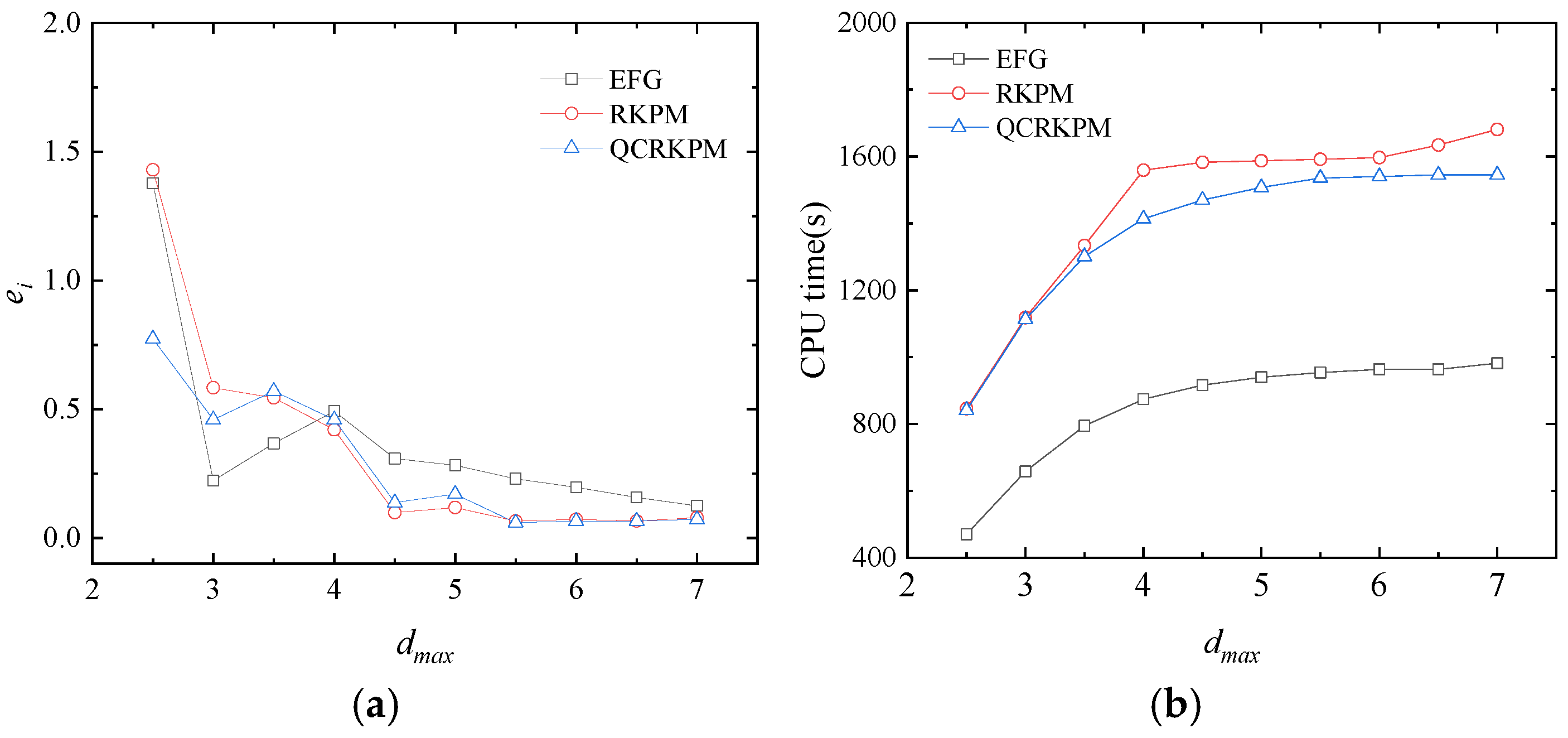
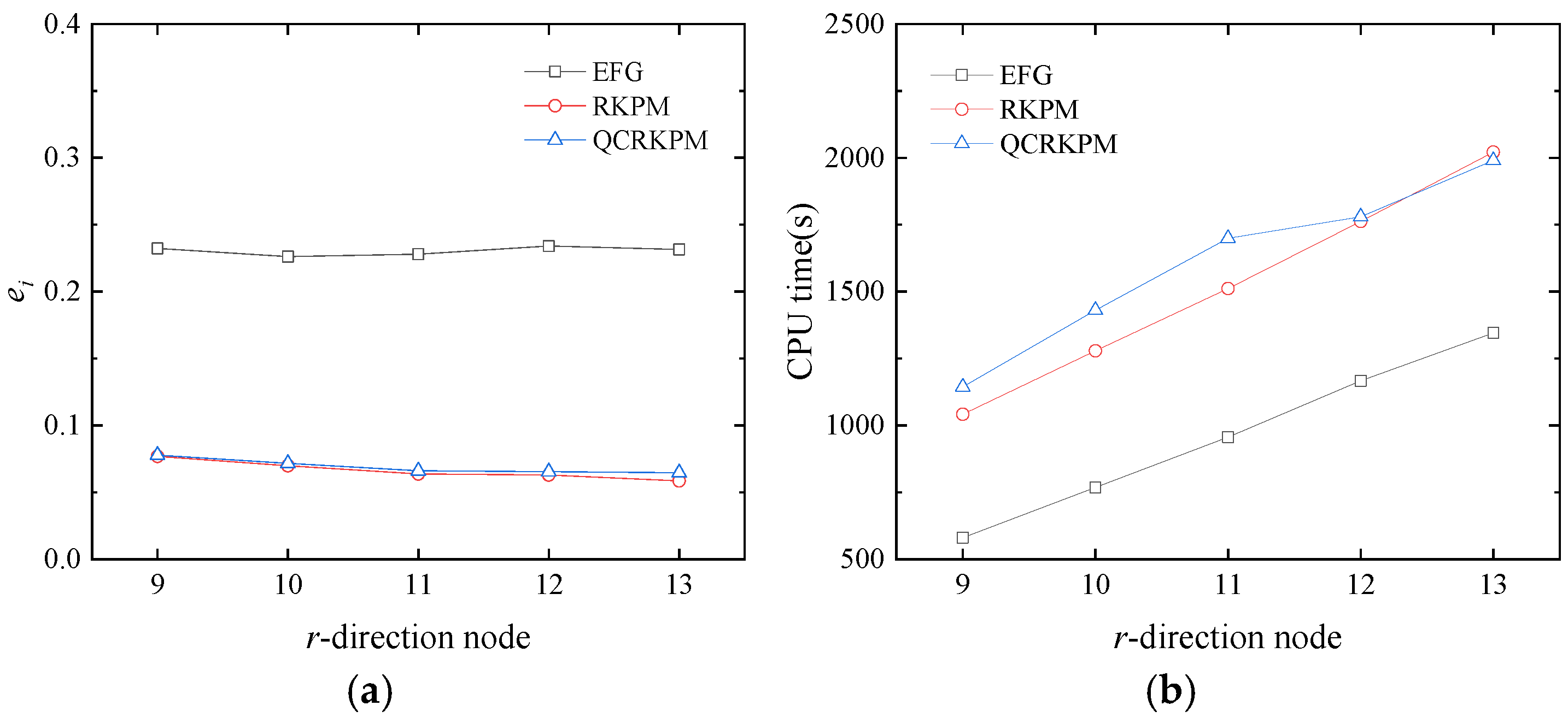
5.1.2. Convergence Study of the Calculation Parameters and Node Distribution of 1/4 Central Hollow Sphere

The effects of the penalty factor α, scaling parameter dmax, and density of node distribution on the computational accuracy and efficiency are investigated in detail. In all cases, the integral background cells are kept still as 8 × 8 × 10. As the QCRKPM employs the penalty method to enforce boundary conditions, the influence of penalty factor α on the numerical accuracy and efficiency is considered first. In this case, 8 × 6 × 11 nodes are used, the scaling parameter dmax, determining the size of the support domain, is 5.5, and the penalty factors α are taken as 2 × 10³, 2 × 10⁴, 2 × 10⁵, 2 × 10⁶, 2 × 10⁷, 2 × 10⁸, 2 × 10⁹, 2 × 10¹⁰, and 2 × 10¹¹, respectively. Figure 6a shows the comparison of the three methods in the overall integral errors with the increase in α. We can see that the QCRKPM has a better accuracy and convergence than the EFG method and a similar performance in terms of accuracy and convergence with the RKPM. From Figure 6b, it can be observed that the value of α does not affect the computational efficiency. Compared with the RKPM, the QCRKPM has a slight efficiency improvement in a certain range of values of α from 2 × 10⁸ to 2 × 10¹¹.
The accuracy and efficiency of the numerical results are also affected by the value of the scaling parameter dmax. In this case, 8 × 6 × 11 nodes are used, and the penalty factor α = 2 × 10⁹ is employed. The scaling parameters dmax are taken as 2.5, 3.0, 3.5, 4.0, 4.5, 5.0, 5.5, 6.0, 6.5, and 7.0, respectively. Figure 7a shows the comparison of the three methods in the overall integral errors with the increase in the dmax. The results show that the QCRKPM has a better accuracy and convergence than the EFG method and a similar performance in terms of accuracy and convergence with the RKPM. The overall integral errors of the RKPM and the QCRKPM are the smallest at dmax = 5.5, which indicates that the accuracy is the highest. The computational time with different scaling parameters dmax is shown in Figure 7b: as the value of dmax increases, the computational time increases gradually. We can see that, compared with the RKPM, the QCRKPM has an obvious computational efficiency advantage.
In addition, to evaluate the influence of the node density on the numerical accuracy and efficiency, the number of nodes in three directions is considered. In this case, the penalty factor α = 2 × 10⁹ and the scaling parameter dmax = 5.5 are employed, the number of nodes in the θ-direction is 6, the number of nodes in the r-direction is 11, and the number of nodes in the φ-direction are 6, 7, 8, 9, and 10, respectively. Figure 8a shows the comparison of the three methods in the overall integral errors with the increase in the number of nodes in the φ-direction. We can see that the QCRKPM has a better accuracy and convergence than the EFG method and the RKPM. It can be seen from Figure 8b that the computational times of the three methods increase with the increase in the number of nodes in the φ-direction, indicating that the computational efficiency decreases gradually, and the result shows that the efficiency of the QCRKPM is comparable with the RKPM’s.
Then, we consider the influence of the number of nodes in the θ-direction on the computational accuracy and efficiency. The number of nodes in the φ-direction is 8, the number of nodes in the r-direction is 11, and the numbers of nodes in the θ-direction are 4, 5, 6, 7, and 8, respectively. Figure 9a compares the three methods’ overall integral errors with the increase in the number of nodes in the θ-direction. We can see that the QCRKPM has a better accuracy and convergence than the EFG method. The results obtained by the QCRKPM are more accurate than those using the RKPM when the number of nodes in the θ-direction does not exceed 6. From Figure 9b, the computational time of the three methods increases with the increase in the number of nodes in the θ-direction, indicating that the computational efficiency decreases gradually, and the result shows the efficiency of the QCRKPM is comparable with the RKPM’s.
Finally, the influence of the number of nodes in the r-direction on the computational accuracy and efficiency is considered. The numbers of nodes are 6 and 8 in the θ-direction and the φ-direction, respectively, and the numbers of nodes in the r-direction are 9, 10, 11, 12, and 13, respectively. The overall integral errors and computational time of the three methods are shown in Figure 10a,b. Figure 10a shows the comparison of the three methods’ overall integral errors with the increase in the number of nodes in the r-direction. The results of the three methods remain unchanged with the increase in the number of nodes in the r-direction, indicating that the change in the number of nodes in the r-direction has little effect on the computational accuracy. From Figure 10a, the computational time of the three methods increases with the increase in the number of nodes in the r-direction, indicating that the computational efficiency decreases gradually.
For this case, we can obtain a preliminary conclusion. The penalty factors α have little effect on the computational precision and efficiency when α exceed 2 × 10⁵. As dmax increases, the overall integral errors decrease and tend to converge. With the increase in the number of nodes in each direction, the computational time is gradually increased. The changes in the number of nodes in the θ-direction and the φ-direction affect the overall integral errors, but the number of nodes in the r-direction has little effect. When the background integral cells are 8 × 8 × 10, the node distribution in the domain of the problem is 8 × 6 × 11, the scaling parameter dmax = 5.5, and the penalty factor α = 2 × 10⁹; satisfactory results can be obtained in terms of the computational accuracy and efficiency.

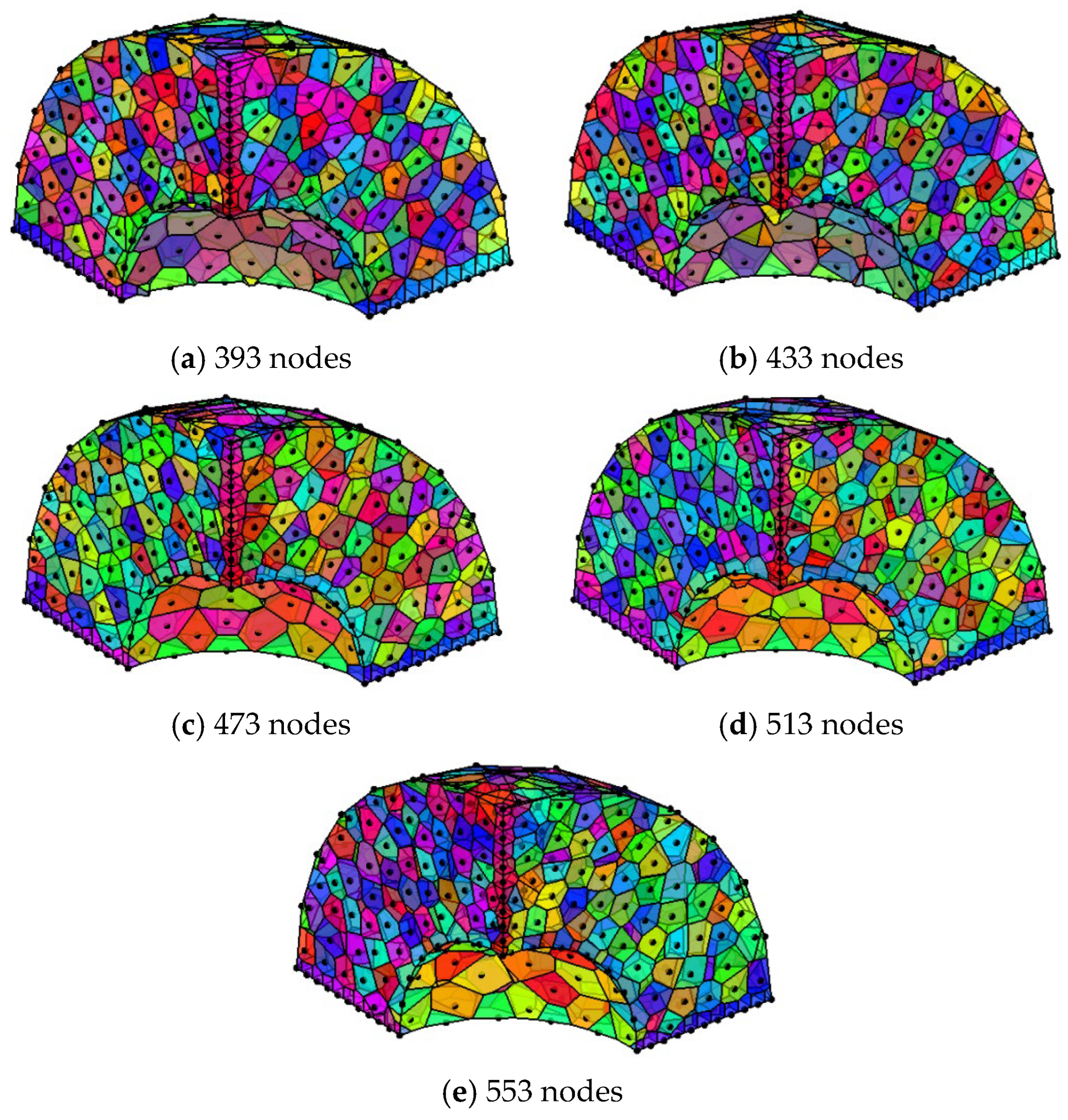
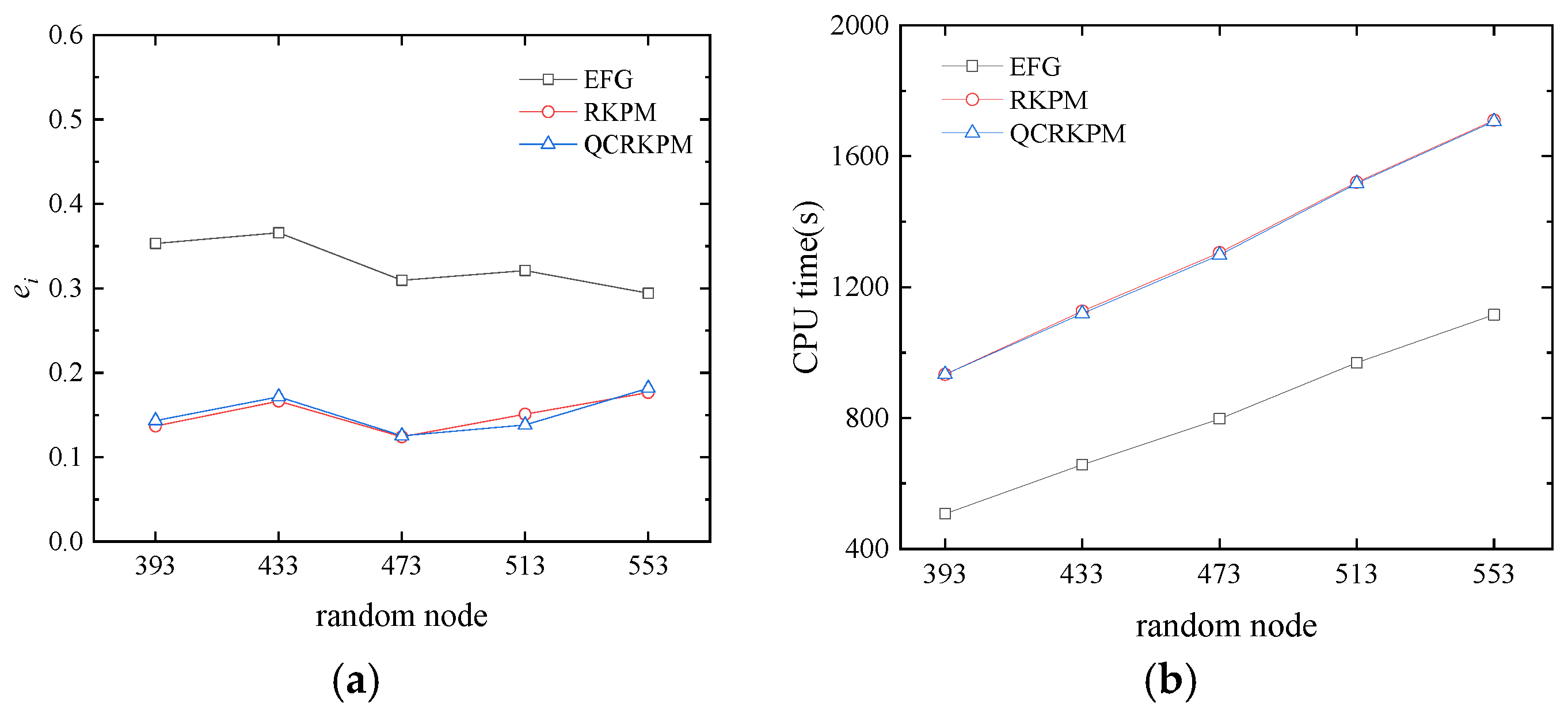
5.1.3. Effects of Random Node Distribution of 1/4 Central Hollow Sphere

As shown in Figure 11, the analysis employs 8 × 8 × 10 background integral cells and five random node modes, which have 393, 433, 473, 513, and 553 nodes, respectively. Computing is performed with the scaling parameters dmax = 5.5 and the penalty factor α = 2 × 10⁹. The relationship between the overall integral errors and number of random nodes is as shown in Figure 12. Numerical results obtained by the QCRKPM are similar to those using the RKPM and are more accurate than the EFG method. When the number of random nodes is 473, the overall integral errors of the three methods reach the minimum, indicating the accuracy is the highest. From Figure 12b, the computational time of the three methods gradually increases with the increase in the number of random nodes, indicating that the computational efficiency gradually decreases. Figure 13 plots the temperature contours obtained by using the analytical solutions and the QCRKPM under the five random placement modes. The results obtained by the present method have an excellent agreement with the analytical solutions.

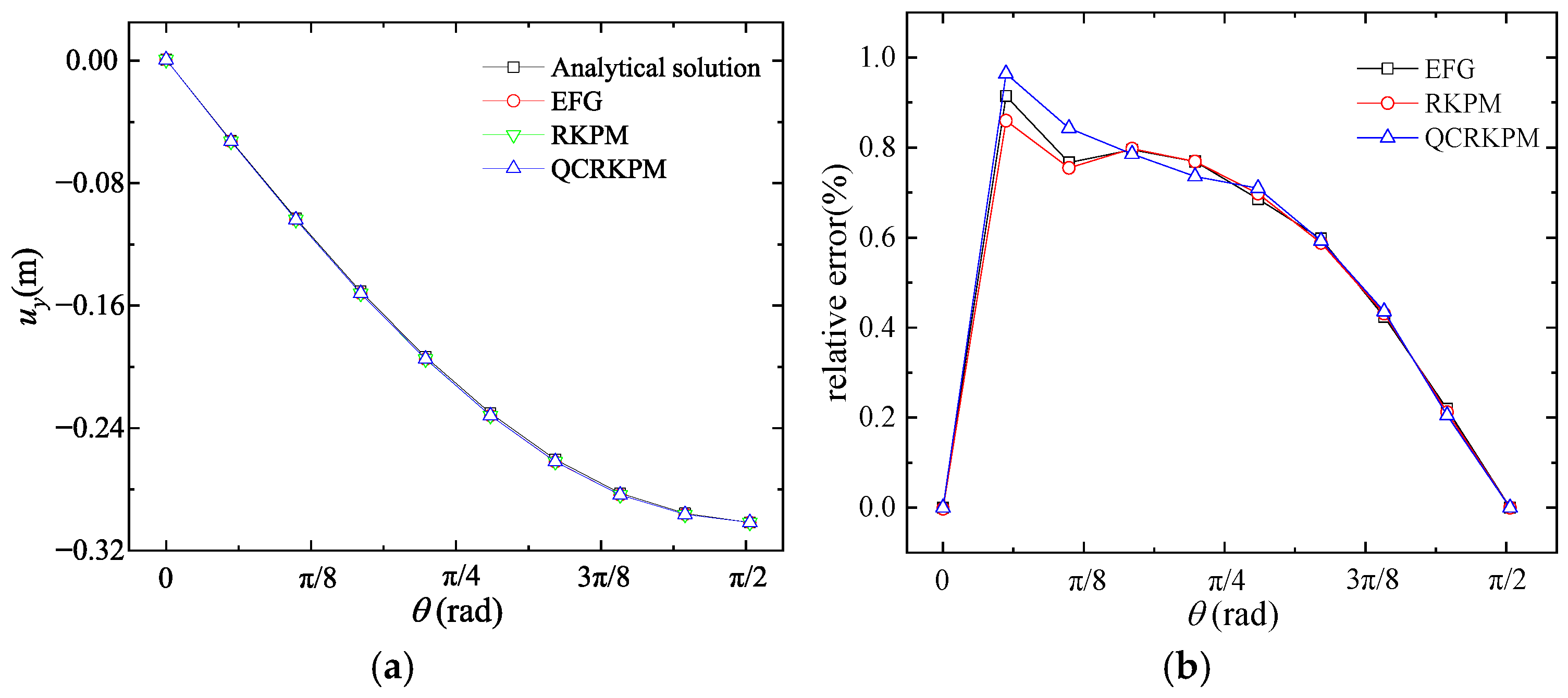
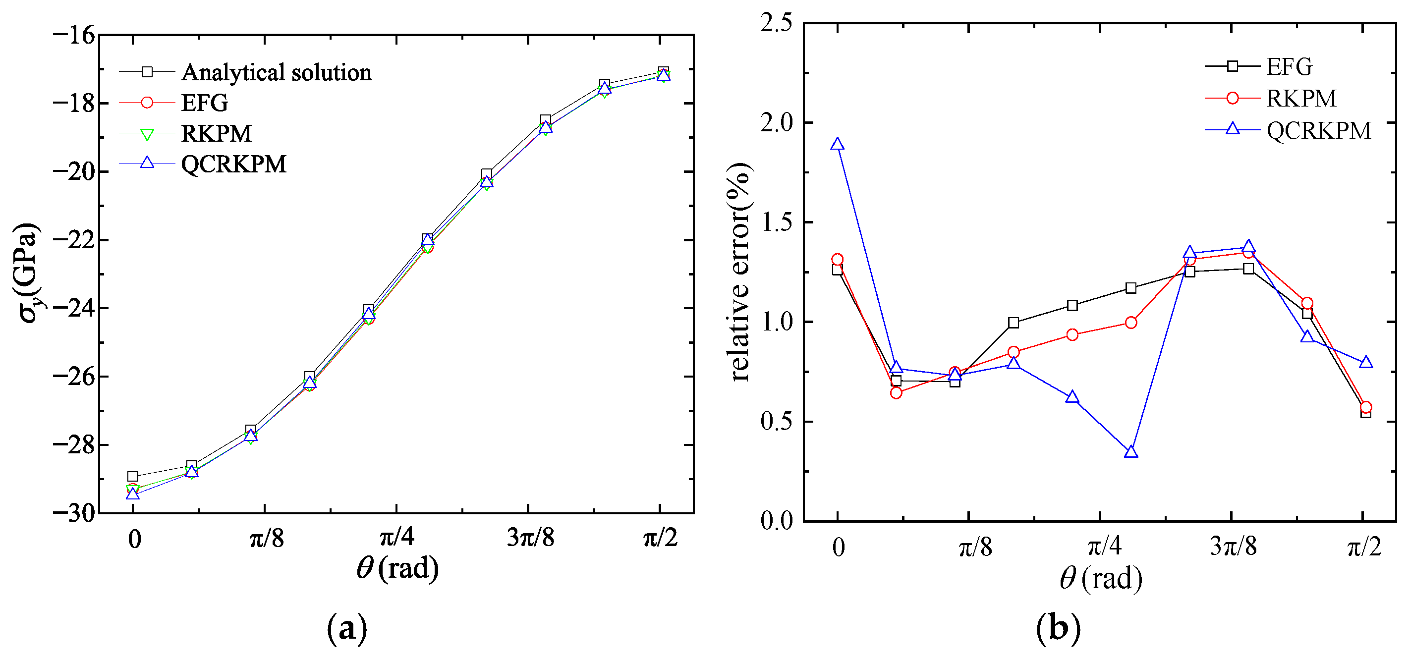
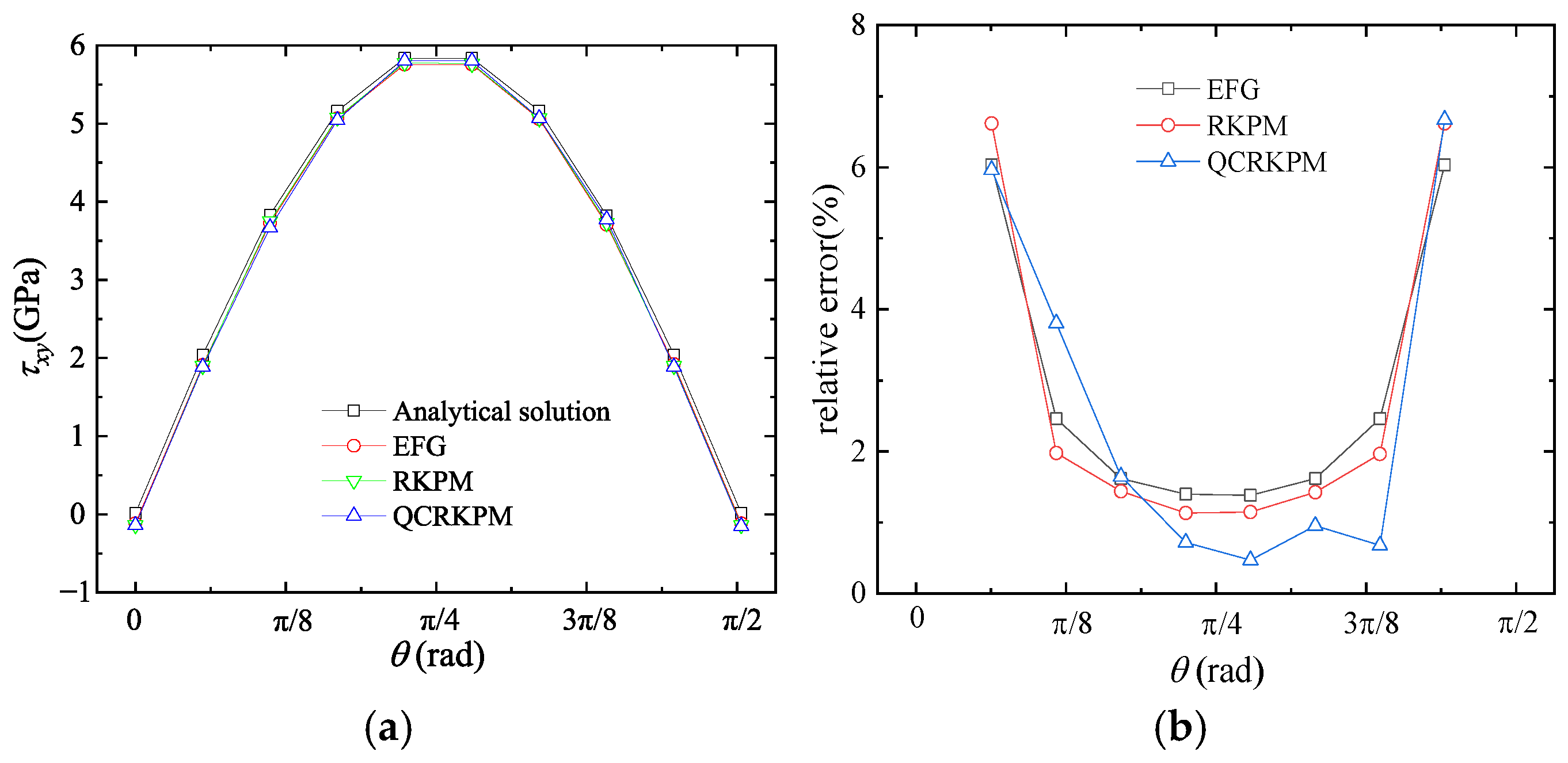
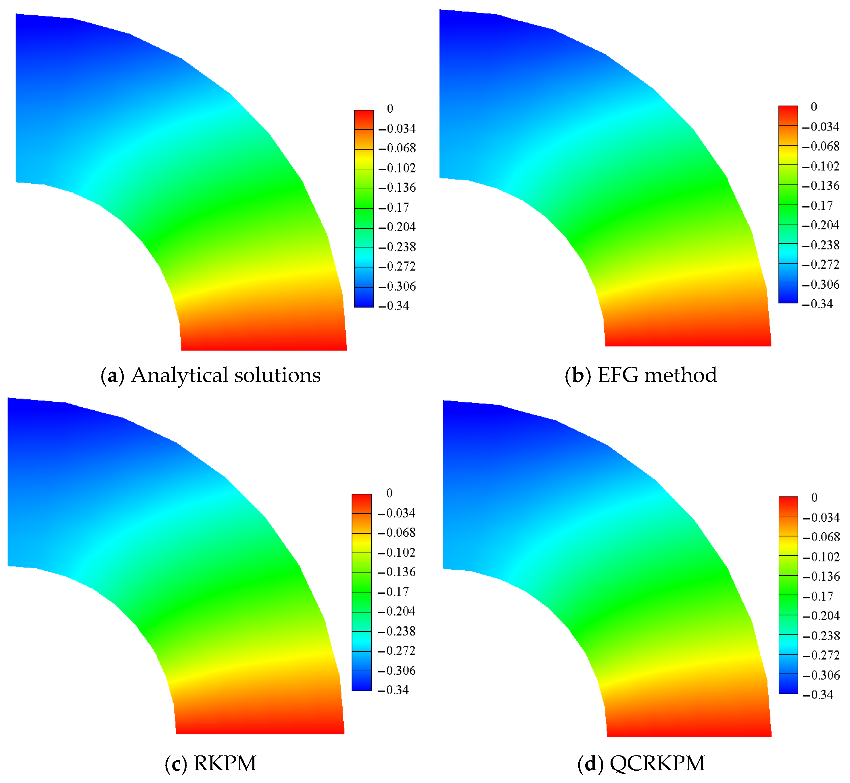
5.2. Steady-State Thermomechanical Coupling Problems on Circular Ring Under Distributed Loads from Inside and Outside

The example considered in this section is a circular ring under distributed loads from inside and outside, and a quarter of the model needs to be considered in the analysis, as shown in Figure 14. The inner and outer diameters are a = 1 m and b = 2 m, and the distributed loads from inside and outside are p a  = 1.0 × 10¹⁰ N/m2 and p b  = 2.0 × 10¹⁰ N/m2, without considering gravity. The problem is considered as in the plane stress state. Poisson’s ratio ν ¯ = ν / ( 1 + v ) , G = 4.80 × 10¹⁰ N/m2, Young’s modulus E = 2 ( 1 + ν ¯ ) G , thermal conductivity coefficient κ = 4.01 Wm−1 K−1, thermal expansion coefficient α ¯ T = α T / ( 1 + ν ¯ ) with Poisson’s ratio v = 0.34 and thermal expansion coefficient α T = 16.5 × 10⁻⁶ K−1 in the plane strain state are used in our analysis. The temperature at the boundaries of the inner and outer circles are T1 = 274.15 K, T2 = 275.15 K. The penalty factors for the heat conduction equation and the thermal stress equation are α, β = α × E, respectively. There is no heat source density inside the circular ring, and the essential boundary conditions are applied by the penalty method.
The analytical solutions [68] for the temperature, displacement, and stress are as follows:
The analytical solutions of the temperature, radial displacement, and circumferential displacement are
T ( x ) = T 2 ln ( x / a ) ln ( b / a ) + T 1 ln ( b / x ) ln ( b / a ) , x Ω
u r ( x ) = γ ¯ 2 1 2 v ¯ 1 v ¯ T 2 T 1 ln ( b / a ) ln x + V 1 v ¯ 1 + v ¯ W 1 x 2 x G , x Ω
u θ = 0
The analytical solutions of stress are
σ x = x 2 + v ¯ y 2 1 v ¯ γ ¯ 2 1 2 v ¯ 1 v ¯ T 2 T 1 ln ( b / a ) 1 x 2 + y 2 + W 1 x 2 + y 2 2 + 2 1 v ¯ γ ¯ 2 1 2 v ¯ 1 v ¯ T 2 T 1 ln ( b / a ) ln x 2 + y 2 + V 1 v ¯ 1 + v ¯ W 1 x 2 + y 2 1 + v ¯ α ¯ T T
σ y = y 2 + v ¯ x 2 1 v ¯ γ ¯ 2 1 2 v ¯ 1 v ¯ T 2 T 1 ln ( b / a ) 1 x 2 + y 2 + W 1 x 2 + y 2 2 + 2 1 v ¯ γ ¯ 2 1 2 v ¯ 1 v ¯ T 2 T 1 ln ( b / a ) ln x 2 + y 2 + V 1 v ¯ 1 + v ¯ W 1 x 2 + y 2 1 + v ¯ α ¯ T T
τ x y = γ ¯ 2 1 2 v ¯ 1 v ¯ T 2 T 1 ln ( b / a ) x y x 2 + y 2 + W 2 x y x 2 + y 2 2
where
γ ¯ = 2 G α ¯ T 1 + v ¯ / 1 2 v ¯
V = p 2 b 2 p 1 a 2 b 2 a 2 , W = p 2 p 1 b 2 a 2 b 2 a 2
p 1 = p a γ ¯ T 1 + γ ¯ 2 T 2 T 1 ln ( b / a ) 1 1 v ¯ ln a + 1
p 2 = p b γ ¯ T 2 + γ ¯ 2 T 2 T 1 ln ( b / a ) 1 1 v ¯ ln b + 1
The temperature boundary conditions are
T x = T 1 , x = a
T x = T 2 , x = b
The heat flux density is
q x = κ T T ln ( b / a ) x n x x 2 , x Ω
The force boundary conditions are
σ x = p a n x , x x Ω | x = a p b n x , x x Ω | x = b
The transformation relationship of the nodal displacement in the polar coordinate system and the Cartesian coordinate system is
u x = u r cos θ u θ sin θ u y = u r sin θ + u θ cos θ

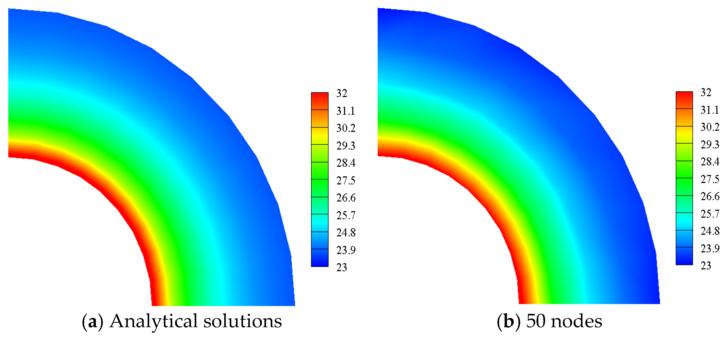
5.2.1. Results of Uniform Node Distribution of 1/4 Circular Ring

As shown in Figure 15, 10 × 8 uniform nodes and 12 × 8 background integral cells are used to discretize the problem domain. The scaling parameter of the influence domain is dmax = 4.0, the penalty factors are α = 104, and β = E × 104 are employed. The numerical results of the radial node temperature at θ = π/4, transverse and vertical displacements at line r = 1.5 m, transverse normal stress, vertical normal stress, and shear stress at line r = 1.5 m, are calculated by using the QCRKPM, the RKPM, and the EFG method, respectively, which are shown in Figure 15, Figure 16, Figure 17, Figure 18, Figure 19 and Figure 20.
The temperature distributions along the radial node at θ = π/4 obtained by analytical solutions and the three meshless methods are illustrated in Figure 16a. Figure 16b shows the relative errors of the three methods on the radial node at θ = π/4. From the comparison results in Figure 16, it is seen that the QCRKPM results are consistent with analytical solutions, and the max relative error of the QCRKPM is less than 0.001%.
In Figure 17 and Figure 18, the transverse and vertical displacements and their relative errors of 10 circumferential nodes at the line r = 1.5 are calculated, respectively. The transverse and vertical displacement obtained by the three methods on the circumferential node at line r = 1.5 m converge to the analytical solutions, and the max relative errors are all less than 1.0%.
As can be seen from Figure 19, Figure 20 and Figure 21, the stress obtained by the three methods on the circumferential node at line r = 1.5 m converge to the analytical solutions. Figure 19 shows that from the third node to the ninth node, the QCRKPM has a higher accuracy in transverse normal stresses σx. In Figure 20 and Figure 21, we can see that on the nodes at the middle part, the QCRKPM has higher accuracy.
Figure 22, Figure 23, Figure 24 and Figure 25 plot the temperature contours, transverse displacement contours, vertical displacement contours, and Von Mises equivalent stress contours, respectively. The results obtained by the QCRKPM have an excellent agreement with the analytical solutions.

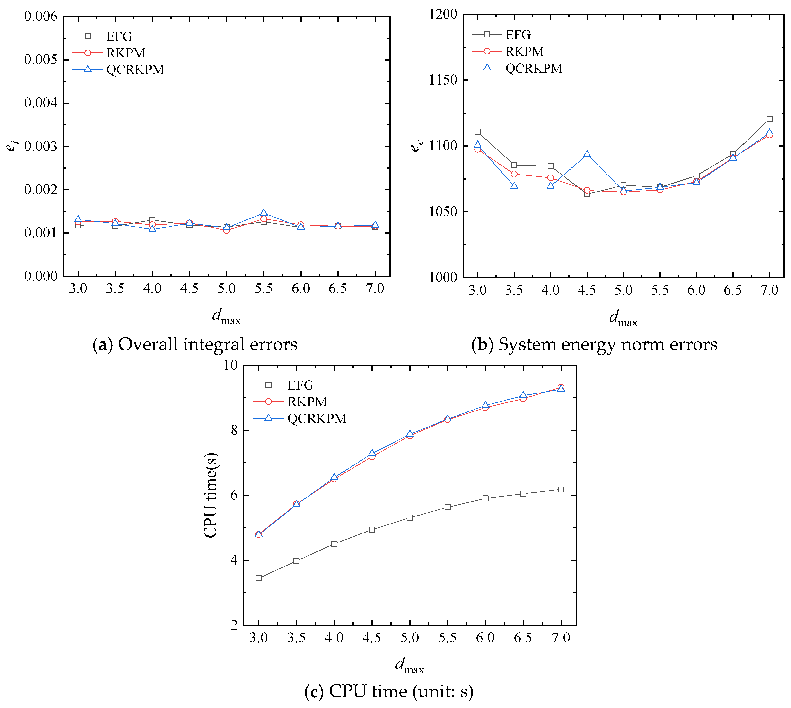
5.2.2. Convergence Study of the Calculation Parameters and Node Distribution in 1/4 Circular Ring

Firstly, to investigate the influence of penalty factor α for the heat conduction equation on the numerical accuracy and efficiency, the values range α = 10, 102, 103, 104, 105, and 106 are employed. The penalty factors for the thermal stress equation are β = α × E; 10 × 8 nodes and 12 × 8 background integral cells are used. The numerical results are for the scaling parameter dmax = 4.0. Figure 26a,b show the comparison of the three methods’ overall integral errors and the system energy norm errors with the increase in α. In Figure 26a, as the value of α increases, the overall integral errors decrease sharply and then converge to zero. In Figure 26b, the system energy norm errors of the three methods also decrease sharply with the increase in α and tend to be stable. In Figure 26c, the computational time of the three methods does not change with the increase in the α, and the computational efficiency of the QCRKPM is close to the RKPM’s.
Secondly, different scaling parameters dmax = 3.0, 3.5, 4.0, 4.5, 5.0, 5.5, 6.0, 6.5, and 7.0 are used to evaluate the influence of dmax on the accuracy and efficiency of numerical results. The background integral cells and the node distribution used are 12 × 8 and 10 × 8, respectively. The penalty factor α = 104 (β = E × α) is employed. The overall integral errors and the system energy norm errors are presented in Figure 27a,b. It can be found that the overall integral errors and the system energy norm errors of the three methods fluctuate slightly with the increase in the dmax. From Figure 27c, the computational time of the three methods increases with the increase in the dmax, which demonstrates the computational efficiency decreases gradually.
Then, we consider the influence of node density on numerical accuracy and efficiency. The penalty factor α (β = E × α) is set as 104, and the scaling parameter dmax is set as 4.0 in a parameter study considering the influence of the number of circumferential node and radial node. The number of radial nodes is 8, the numbers of circumferential nodes are 8, 9, 10, 11, and 12, respectively. With these nodes, 10 × 8 background integral cells are used. The comparison of the three methods in the overall integral errors and the system energy norm errors with the increase in the number of circumferential nodes is shown in Figure 28a,b. It can be found that the overall integral errors and the system energy norm errors of the three methods fluctuate, and the overall integral errors converge to zero with the increase in circumferential node. From Figure 28c, the computational time of the three meshless methods slowly increases with the increase in the circumferential node, indicating that the computational efficiency gradually decreases.
The influence of the number of radial nodes is considered at last. The number of circumferential nodes is 10, and the number of radial nodes are 5, 6, 7, 8, and 9, respectively; 10 × 8 background integral cells are employed. Figure 29a,b show the comparison of the three meshless methods’ overall integral errors and the system energy norm errors with the increase in the number of radial nodes. In Figure 29a, the overall integral errors of the three methods fluctuate and tend to zero with the increase in the number of radial nodes, and when the number of radial nodes is 8, the overall integral errors of the three methods are smaller, indicating that the computational precision is higher. In Figure 29b, the system energy norm errors of the three methods decrease sharply and then increase slowly with the increase in the number of radial nodes. When the number of radial nodes is 7, the system energy norm errors of the RKPM and the QCRKPM is the smallest, which indicates the highest computational accuracy. In Figure 29c, the computational time of the three methods increases with the number of radial nodes, indicating that the computational efficiency gradually decreases.
For this case, we can also obtain a preliminary conclusion. The penalty factors α have little effect on the computational accuracy and efficiency when α exceed 102. As the dmax changes, the overall integral errors and system energy norm errors fluctuate slightly and tend to converge. The value of α and the number of circumferential nodes have little effect on the computational efficiency, while the value of dmax and the number of circumferential nodes have a great influence. When the node distribution is 10 × 8, the background integral mesh is 12 × 8, the scaling parameter dmax = 4.0, and the penalty factors α = 104 and β = E × 104; satisfactory results can be obtained in terms of the computational accuracy and efficiency.

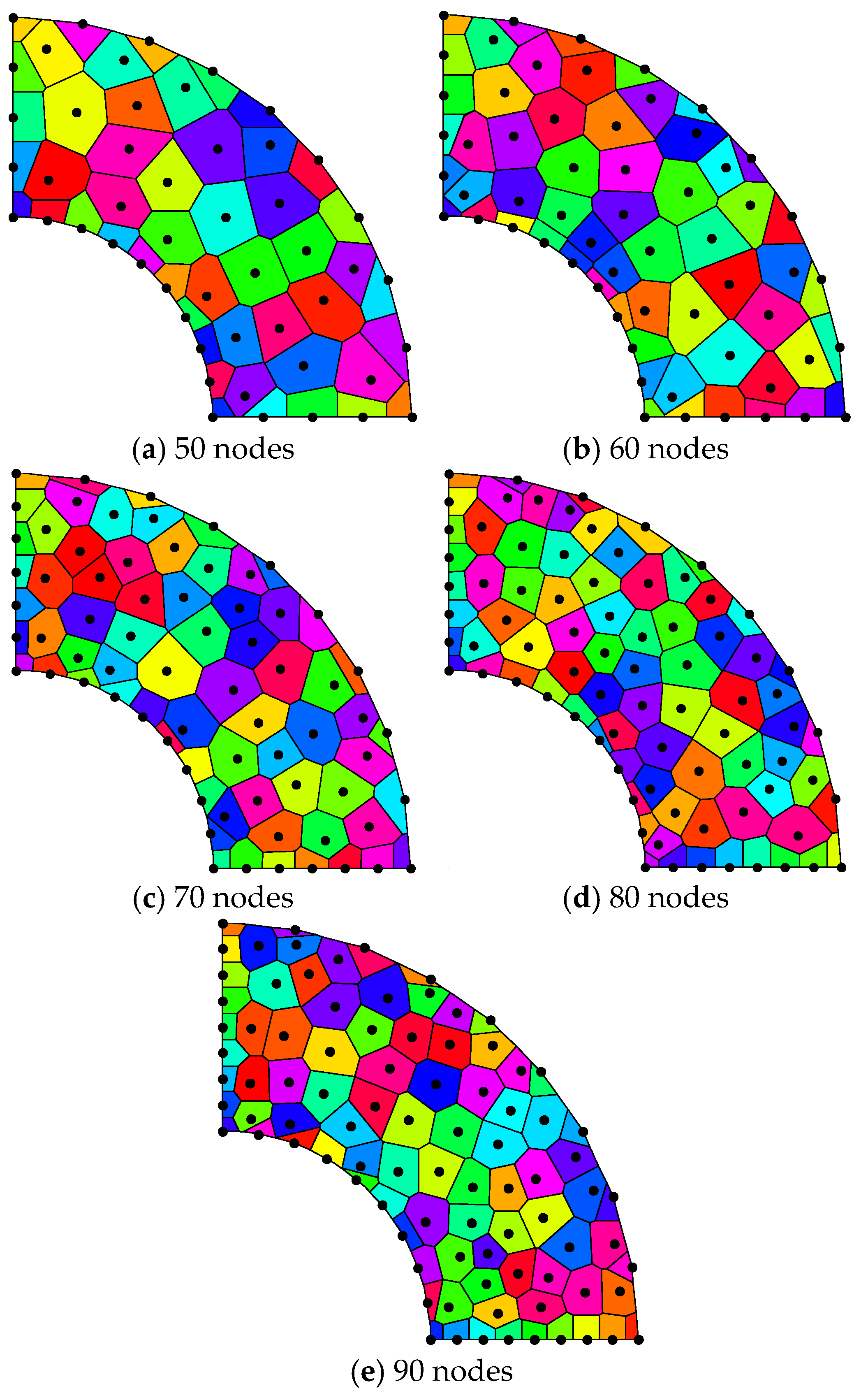
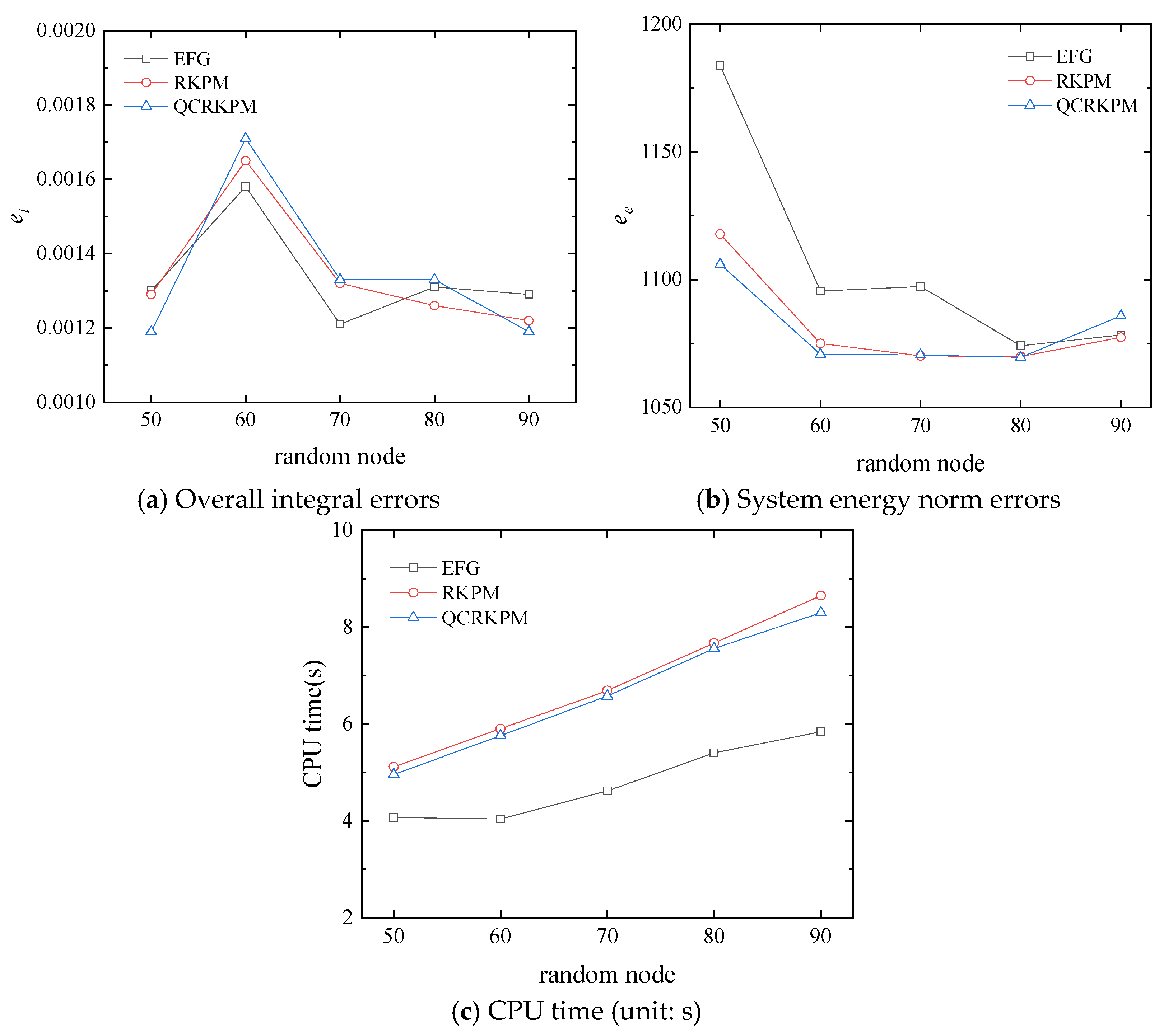
5.2.3. Effects of Random Node Distribution of 1/4 Circular Ring

The random node distribution in the problem domain is carried out in five modes, which have 50, 60, 70, 80, and 90 nodes, respectively, as shown in Figure 30. The analysis employs 12 × 8 background integral cells. The numerical results are for the scaling parameter dmax = 4.0, the penalty factor α = 104 and β = E × 104, and the number of random nodes is taken as the above five modes, respectively. The overall integral errors, system energy norm errors, and computational time under the different modes are shown in Figure 31.
In Figure 31a, the overall integral errors of the RKPM and the QCRKPM increase with the number of nodes and then decrease before stabilizing, while the overall integral errors of the EFG method fluctuate with the number of random nodes. When the number of random nodes is 70, the overall integral errors of the three methods are smaller, indicating a higher accuracy. In Figure 31b, the system energy norm errors for the RKPM and the QCRKPM decrease and then increase slowly as the number of random nodes increases, while the system energy norm errors for the EFG method fluctuate as the number of random nodes increases. When the number of nodes is 80, the overall integral errors for the three methods are small, indicating high precision. In Figure 31c, the computational time of the three methods gradually increases with the number of random nodes, indicating that the computational efficiency gradually decreases. We can also see that the computational efficiency of the QCRKPM is slightly improved compared to RKPM. The temperature contours and Von Mises equivalent stress contours obtained by using analytical solutions and the QCRKPM under the five random node modes are plotted in Figure 32 and Figure 33. The numerical results obtained by using the QCRKPM agree well with the analytical solutions.

6. Conclusions

In this paper, a numerical strategy for steady-state thermomechanical coupling problems using the quasi-convex reproducing kernel particle method is developed. The Galerkin weak form is employed to derive the equations system, and the penalty method is used to apply the essential boundary conditions. The discrete equations of the QCRKPM for the thermomechanical coupling problems are derived. The nearly convex shape functions of the QCRK approximation help improve the positivity of some thermal matrixes in the final discreated equations. The computational accuracy and efficiency are investigated for the different computing parameters, namely the scaling parameter of the influence domain, the penalty factor, and the node distribution density, in both uniform and random ways. The results indicate that the QCRKPM demonstrates stability and satisfactory accuracy for the temperature, stress, and displacement solutions under the tested computing parameters, including the influence domain scaling factor, the penalty factor, and the node distribution. Compared with the EFG method and the RKPM, the QCRKPM for thermomechanical coupling problems could slightly improve the computational accuracy without reducing the computational efficiency of the shape function and its first-order partial derivative. Our findings help lay the foundation for further development of transient thermomechanical coupling in complex conditions.

Author Contributions

Conceptualization, D.M.L.; Methodology, D.M.L.; Investigation, L.Z. and L.-R.T.; Writing—original draft, L.Z., D.M.L., C.-Y.L. and L.-R.T.; Writing—review & editing, D.M.L. All authors have read and agreed to the published version of the manuscript.

Funding

The supports of the Natural Science Foundation of Hubei Province (2018CFB129) and the Fundamental Research Funds for the Central Universities of China (WUT: 2016IVA022 and WUT: 2021IVB013) are acknowledged.

Data Availability Statement

The original contributions presented in this study are included in the article. Further inquiries can be directed to the corresponding author.

Conflicts of Interest

The authors declare no conflict of interest.

References

  1. Deng, Y.B.; Wu, Y.W.; Zhang, D.L.; Lu, Q.; Tian, W.X.; Qiu, S.; Su, G.H. Thermal-mechanical coupling behavior analysis on metal-matrix dispersed plate-type fuel. Prog. Nucl. Energy 2017, 95, 8–22. [Google Scholar] [CrossRef]
  2. Zhang, L.; Liu, J.H.; Wu, X.Q.; Zhuang, C. Digital twin-based dynamic prediction of thermomechanical coupling for skiving process. Int. J. Adv. Manuf. Technol. 2012, 131, 5471–5488. [Google Scholar] [CrossRef]
  3. Li, Y.; Cui, X.F.; Tan, N.; Li, Q. Evolution of microstructure and performance of plasma cladding coating and interface with thermomechanical coupling effects. Surf. Eng. 2010, 36, 695–705. [Google Scholar] [CrossRef]
  4. Ghasemi, M.A.; Falahatgar, S.R.; Mostof, T.M. Mechanical and thermomechanical mesoscale analysis of multiple surface cracks in ceramic coatings based on the DEM-FEM coupling method. Int. J. Solids Struct. 2012, 236, 111336. [Google Scholar] [CrossRef]
  5. Joulin, C.; Xiang, J.S.; Latham, J.P. A novel thermo-mechanical coupling approach for thermal fracturing of rocks in the three-dimensional FDEM. Comput. Part. Mech. 2010, 7, 935–946. [Google Scholar] [CrossRef]
  6. Zhao, S.W.; Zhao, J.D.; Lai, Y.M. Multiscale modeling of thermo-mechanical responses of granular materials: A hierarchical continuum–discrete coupling approach. Comput. Methods Appl. Mech. Eng. 2010, 367, 113100. [Google Scholar] [CrossRef]
  7. Belytschko, T.; Kronggauz, Y.; Organ, D.; Fleming, M. Meshless methods: An overview and recent developments. Comput. Methods Appl. Mech. Eng. 1996, 139, 3–47. [Google Scholar] [CrossRef]
  8. Liu, G.R. Mesh Free Methods: Moving Beyond the Finite Element Method, 2nd ed.; CRC Press: Boca Raton, FL, USA, 2019. [Google Scholar]
  9. Monaghan, J.J. Smoothed particle hydrodynamics. Annu. Rev. Astron. Astrophys. 1992, 30, 543–574. [Google Scholar] [CrossRef]
  10. Nayroles, B.; Touzot, G.; Villon, P. Generalizing the finite element method: Diffuse approximation and diffuse elements. Comput. Mech. 1992, 10, 307–318. [Google Scholar] [CrossRef]
  11. Belytschko, T.; Lu, Y.Y.; Gu, L. Element-free Galerkin methods. Int. J. Numer. Methods Eng. 1994, 37, 229–256. [Google Scholar] [CrossRef]
  12. Liu, W.K.; Jun, S.; Zhang, Y.F. Reproducing kernel particle methods. Int. J. Numer. Methods Fluids 1995, 20, 1081–1106. [Google Scholar] [CrossRef]
  13. Atluri, S.N.; Zhu, T. A new meshless local Petrov-Galerkin (MLPG) approach in computational mechanics. Comput. Mech. 1998, 22, 117–127. [Google Scholar] [CrossRef]
  14. Wang, J.G.; Liu, G.R. A point interpolation meshless method based on radial basis functions. Int. J. Numer. Methods Eng. 2012, 54, 1623–1648. [Google Scholar] [CrossRef]
  15. Gu, L. Moving kriging interpolation and element-free Galerkin method. Int. J. Numer. Methods Eng. 2013, 56, 1–11. [Google Scholar] [CrossRef]
  16. Chen, J.S.; Hu, W.; Hu, H.Y. Reproducing kernel enhanced local radial basis collocation method. Int. J. Numer. Methods Eng. 2018, 75, 600–627. [Google Scholar] [CrossRef]
  17. Sukumar, N. Construction of polygonal interpolants: A maximum entropy approach. Int. J. Numer. Methods Eng. 2014, 61, 2159–2181. [Google Scholar] [CrossRef]
  18. Li, D.; Bai, F.N.; Cheng, Y.M.; Liew, K.M. A novel complex variable element-free Galerkin method for two-dimensional large deformation problems. Comput. Methods Appl. Mech. Eng. 2012, 233–236, 1–10. [Google Scholar] [CrossRef]
  19. Wang, D.D.; Chen, P.J. Quasi-convex reproducing kernel meshfree method. Comput. Mech. 2014, 54, 689–709. [Google Scholar] [CrossRef]
  20. Li, D.M.; Zhang, L.W.; Liew, K.M. A three-dimensional element-free framework for coupled mechanical-diffusion induced nonlinear deformation of polymeric gels using the IMLS-Ritz method. Comput. Methods Appl. Mech. Eng. 2015, 296, 232–247. [Google Scholar] [CrossRef]
  21. Chen, J.S.; Pan, C.; Wu, C.T.; Liu, W.K. Reproducing Kernel Particle Methods for large deformation analysis of non-linear structures. Comput. Methods Appl. Mech. Eng. 1996, 139, 195–227. [Google Scholar] [CrossRef]
  22. Li, S.; Hao, W.; Liu, W.K. Mesh-free simulations of shear banding in large deformation. Int. J. Solids Struct. 2010, 37, 7185–7206. [Google Scholar] [CrossRef]
  23. Liew, K.M.; Ng, T.Y.; Wu, Y.C. Meshfree method for large deformation analysis–A reproducing kernel particle approach. Eng. Struct. 2012, 24, 543–551. [Google Scholar] [CrossRef]
  24. Li, D.M.; Zhang, Z.; Liew, K.M. A numerical framework for two-dimensional large deformation of inhomogeneous swelling of gels using the improved complex variable element-free Galerkin method. Comput. Methods Appl. Mech. Eng. 2014, 274, 84–102. [Google Scholar] [CrossRef]
  25. Li, D.M.; Liew, K.M.; Cheng, Y.M. An improved complex variable element-free Galerkin method for two-dimensional large deformation elastoplasticity problems. Comput. Methods Appl. Mech. Eng. 2014, 269, 72–86. [Google Scholar] [CrossRef]
  26. Li, D.M.; Kong, L.H.; Liu, J.H. A generalized decoupling numerical framework for polymeric gels and its element-free implementation. Int. J. Numer. Methods Eng. 2010, 121, 2701–2726. [Google Scholar] [CrossRef]
  27. Li, D.M.; Featherston, C.A.; Wu, Z. An element-free study of variable stiffness composite plates with cutouts for enhanced buckling and post-buckling performance. Comput. Methods Appl. Mech. Eng. 2010, 371, 113314. [Google Scholar] [CrossRef]
  28. Fleming, M.; Chu, Y.A.; Moran, B.; Belytschko, T. Enriched element-free Galerkin methods for crack tip fields. Int. J. Numer. Methods Eng. 1997, 40, 1483–1504. [Google Scholar] [CrossRef]
  29. Rao, B.N.; Rahman, S. An efficient meshless method for fracture analysis of cracks. Comput. Mech. 2010, 26, 398–408. [Google Scholar] [CrossRef]
  30. Rabczuk, T.; Belytschko, T. Cracking particles: A simplified meshfree method for arbitrary evolving cracks. Int. J. Numer. Methods Eng. 2014, 61, 2316–2343. [Google Scholar] [CrossRef]
  31. Sun, Y.; Hu, Y.G.; Liew, K.M. A mesh-free simulation of cracking and failure using the cohesive segments method. Int. J. Eng. Sci. 2017, 45, 541–553. [Google Scholar] [CrossRef]
  32. Peng, Y.X.; Zhang, A.M.; Ming, F.R. A 3D meshfree crack propagation algorithm for the dynamic fracture in arbitrary curved shell. Comput. Methods Appl. Mech. Eng. 2010, 367, 113139. [Google Scholar] [CrossRef]
  33. Li, D.M.; Liu, J.H.; Nie, F.H.; Featherston, C.A.; Wu, Z. On tracking arbitrary crack path with complex variable meshless methods. Comput. Methods Appl. Mech. Eng. 2012, 399, 115402. [Google Scholar] [CrossRef]
  34. Pan, J.H.; Li, D.M.; Luo, X.B.; Zhu, W. An enriched improved complex variable element-free Galerkin method for efficient fracture analysis of orthotropic materials. Theor. Appl. Fract. Mech. 2012, 121, 103488. [Google Scholar] [CrossRef]
  35. Pan, J.H.; Li, D.M.; Cai, S.; Luo, X.B. A pure complex variable enrichment method for modeling progressive fracture of orthotropic functionally gradient materials. Eng. Fract. Mech. 2013, 277, 108984. [Google Scholar] [CrossRef]
  36. Zhang, G.M.; Batra, R.C. Modified smoothed particle hydrodynamics method and its application to transient problems. Comput. Mech. 2014, 34, 137–146. [Google Scholar] [CrossRef]
  37. Liu, Y.; Zhang, X.; Lu, M.W. A meshless method based on least-squares approach for steady- and unsteady-state heat conduction problems. Numer. Heat Transf. Part B Fundam. 2015, 47, 257–275. [Google Scholar] [CrossRef]
  38. Qian, L.; Batra, R. Three-Dimensional transient heat conduction in a functionally graded thick plate with a higher-order plate theory and a meshless local Petrov-Galerkin method. Comput. Mech. 2015, 35, 214–226. [Google Scholar] [CrossRef]
  39. Singh, A.; Singh, I.V.; Prakash, R. Meshless element free Galerkin method for unsteady nonlinear heat transfer problems. Int. J. Heat Mass Transf. 2017, 50, 1212–1219. [Google Scholar] [CrossRef]
  40. Nakonieczny, K.; Sadowski, T. Modelling of thermal shocks in composite materials using a meshfree FEM. Comput. Mater. Sci. 2019, 44, 1307–1311. [Google Scholar] [CrossRef]
  41. Cheng, R.; Liew, K.M. The reproducing kernel particle method for two-dimensional unsteady heat conduction problems. Comput. Mech. 2019, 45, 1–10. [Google Scholar] [CrossRef]
  42. Cao, L.; Qin, Q.H.; Zhao, N. An RBF-MFS model for analysing thermal behavior of skin tissues. Int. J. Heat Mass Transf. 2010, 53, 1298–1307. [Google Scholar] [CrossRef]
  43. Tang, J.D.; He, Z.H.; Liu, H.; Dong, S.K.; Tan, H.P. Reproducing kernel particle method for coupled conduction-radiation phase-change heat transfer. Int. J. Heat Mass Transf. 2018, 120, 387–398. [Google Scholar] [CrossRef]
  44. Li, J.; Wang, G.; Zhan, J.; Liu, S.; Guan, Y.; Naceur, H.; Coutellier, D.; Lin, J. Meshless SPH analysis for transient heat conduction in the functionally graded structures. Compos. Commun. 2011, 24, 100664. [Google Scholar] [CrossRef]
  45. Guan, Y.; Atluri, S.N. Meshless fragile points methods based on Petrov-Galerkin weak-forms for transient heat conduction problems in complex anisotropic nonhomogeneous media. Int. J. Numer. Methods Eng. 2011, 122, 4055–4092. [Google Scholar] [CrossRef]
  46. Sládek, J.; Sládek, V.; Atluri, S.N. A pure contour formulation for the meshless local boundary integral equation method in thermoelasticity. Cmes-Comput. Model. Eng. Sci. 2011, 2, 423–434. [Google Scholar]
  47. Bobaru, F.; Mukherjee, S. Meshless approach to shape optimization of linear thermoelastic solids. Int. J. Numer. Methods Eng. 2012, 53, 765–796. [Google Scholar] [CrossRef]
  48. Qian, L.F.; Batra, R.C.; Chen, L.M. Analysis of cylindrical bending thermoelastic deformations of functionally graded plates by a meshless local Petrov-Galerkin method. Comput. Mech. 2014, 33, 263–273. [Google Scholar] [CrossRef]
  49. Qian, L.F.; Batra, R.C. Transient thermoelastic deformations of a thick functionally graded plate. J. Therm. Stress. 2014, 27, 705–740. [Google Scholar] [CrossRef]
  50. Chen, J. Determination of thermal stress intensity factors for an interface crack in a graded orthotropic coating- substrate structure. Int. J. Fract. 2015, 133, 303–328. [Google Scholar] [CrossRef]
  51. Ching, H.K.; Yen, S.C. Meshless local Petrov-Galerkin analysis for 2D functionally graded elastic solids under mechanical and thermal loads. Compos. Part B Eng. 2015, 36, 223–240. [Google Scholar] [CrossRef]
  52. Ching, H.K.; Yen, S.C. Transient thermoelastic deformations of 2-D functionally graded beams under nonuniformly convective heat supply. Compos. Struct. 2016, 73, 381–393. [Google Scholar] [CrossRef]
  53. Wang, H.; Qin, Q.H. Meshless approach for thermo-mechanical analysis of functionally graded materials. Eng. Anal. Bound. Elem. 2018, 32, 704–712. [Google Scholar] [CrossRef]
  54. Zheng, B.J.; Gao, X.W.; Yang, K.; Zhang, C.Z. A novel meshless local Petrov-Galerkin method for dynamic coupled thermoelasticity analysis under thermal and mechanical shock loading. Eng. Anal. Bound. Elem. 2015, 60, 154–161. [Google Scholar] [CrossRef]
  55. Vaghefi, R.; Hematiyan, M.R.; Nayebi, A. Three-dimensional thermo-elastoplastic analysis of thick functionally graded plates using the meshless local Petrov-Galerkin method. Eng. Anal. Bound. Elem. 2016, 71, 34–49. [Google Scholar] [CrossRef]
  56. Memari, A.; Azar, M.R.K. Thermo-mechanical shock fracture analysis by meshless method. Theor. Appl. Fract. Mech. 2019, 102, 171–192. [Google Scholar] [CrossRef]
  57. Khosravifard, A.; Hematiyan, M.R.; Ghiasi, N. A meshfree method with dynamic node reconfiguration for analysis of thermo-elastic problems with moving concentrated heat sources. Appl. Math. Model. 2010, 79, 624–638. [Google Scholar] [CrossRef]
  58. Hillman, M.; Lin, K.C. Nodally integrated thermomechanical RKPM: Part I—Thermoelasticity. Comput. Mech. 2011, 68, 795–820. [Google Scholar] [CrossRef]
  59. Hillman, M.; Lin, K.C. Nodally integrated thermomechanical RKPM: Part II—Generalized thermoelasticity and hyperbolic finite-strain thermoplasticity. Comput. Mech. 2011, 68, 821–844. [Google Scholar] [CrossRef]
  60. Reséndiz-Flores, E.O.; Saucedo-Zendejo, F.R.; Jiménez-Villalpando, A.V. Fully coupled meshfree numerical approach based on the finite pointset method for static linear thermoelasticity problems. Comput. Part. Mech. 2012, 9, 237–250. [Google Scholar] [CrossRef]
  61. Saucedo-Zendejo, F.R.; Reséndiz-Flores, E.O. Meshfree numerical approach based on the finite pointset method for two-way coupled transient linear thermoelasticity. Comput. Part. Mech. 2013, 10, 289–302. [Google Scholar] [CrossRef]
  62. Shukla, V.; Singh, J. Thermo-mechanical stability analysis of angle-ply plates using meshless method. Appl. Math. Comput. 2012, 413, 126644. [Google Scholar] [CrossRef]
  63. Wu, C.T.; Park, C.K.; Chen, J.S. A generalized approximation for the meshfree analysis of solids. Int. J. Numer. Methods Eng. 2011, 85, 693–722. [Google Scholar] [CrossRef]
  64. Arroyo, M.; Ortiz, M. Local maximum-entropy approximation schemes: A seamless bridge between finite elements and meshfree methods. Int. J. Numer. Methods Eng. 2016, 65, 2167–2202. [Google Scholar] [CrossRef]
  65. Zhang, H.J.; Wang, D.D. An isogeometric enriched quasi-convex meshfree formulation with application to material interface modeling. Eng. Anal. Bound. Elem. 2015, 60, 37–50. [Google Scholar] [CrossRef]
  66. Zhang, H.J.; Wu, J.Z.; Wang, D.D. Free vibration analysis of cracked thin plates by quasi-convex coupled isogeometric-meshfree method. Front. Struct. Civ. Eng. 2015, 9, 405–419. [Google Scholar] [CrossRef]
  67. Wang, F.J.; Chen, W.; Qu, W.Z.; Gu, Y. A BEM formulation in conjunction with parametric equation approach for three-dimensional Cauchy problems of steady heat conduction. Eng. Anal. Bound. Elem. 2016, 63, 1–14. [Google Scholar] [CrossRef]
  68. Marin, L.; Karageorghis, A. The MFS-MPS for two-dimensional steady-state thermoelasticity problems. Eng. Anal. Bound. Elem. 2013, 37, 1004–1020. [Google Scholar] [CrossRef]
Figure 1. The flowchart of QCRKPM.
Mathematics 13 02259 g001
Figure 2. The central hollow sphere.
Mathematics 13 02259 g002
Figure 3. Node distribution of 1/4 central hollow sphere.
Mathematics 13 02259 g003
Figure 4. (a) Temperature (unit: K) and (b) corresponding relative errors of nodes at θ = π/4 and φ = π/4.
Mathematics 13 02259 g004
Figure 5. Temperature contours of 1/4 central hollow sphere (unit: K).
Mathematics 13 02259 g005
Figure 6. (a) Overall integral errors and (b) CPU time (unit: s) with different penalty factors α.
Mathematics 13 02259 g006
Figure 7. (a) Overall integral errors and (b) CPU time (unit: s) with different scaling parameters dmax.
Mathematics 13 02259 g007
Figure 8. (a) Overall integral errors and (b) CPU time (unit: s) versus φ-direction node.
Mathematics 13 02259 g008
Figure 9. (a) Overall integral errors and (b) CPU time (unit: s) versus θ-direction node.
Mathematics 13 02259 g009
Figure 10. (a) Overall integral errors and (b) CPU time (unit: s) versus r-direction node.
Mathematics 13 02259 g010
Figure 11. Random nodes of 1/4 central hollow sphere.
Mathematics 13 02259 g011
Figure 12. (a) Overall integral errors and (b) CPU time (unit: s) with random nodes.
Mathematics 13 02259 g012
Figure 13. Temperature contours of the central hollow sphere with random nodes (unit: K).
Mathematics 13 02259 g013
Figure 14. 1/4 thermoelastic circular ring under distributed loads from inside and outside.
Mathematics 13 02259 g014
Figure 15. Node distribution of 1/4 circular ring.
Mathematics 13 02259 g015
Figure 16. (a) Temperature (unit: K) and (b) corresponding relative errors for nodes at θ = π/4.
Mathematics 13 02259 g016
Figure 17. (a) ux (unit: m) and (b) corresponding relative errors for nodes at r = 1.5 m.
Mathematics 13 02259 g017
Figure 18. (a) uy (unit: m) and (b) corresponding relative errors for nodes at r = 1.5 m.
Mathematics 13 02259 g018
Figure 19. (a) σx (unit: GPa) and (b) corresponding relative errors for nodes at r = 1.5 m.
Mathematics 13 02259 g019
Figure 20. (a) σy (unit: GPa) and (b) corresponding relative errors for nodes at r = 1.5 m.
Mathematics 13 02259 g020
Figure 21. (a) τxy (unit: GPa) and (b) corresponding relative errors for nodes at r = 1.5 m.
Mathematics 13 02259 g021
Figure 22. Temperature contours with uniform nodes (unit: K).
Mathematics 13 02259 g022
Figure 23. Transverse displacement contours (unit: m).
Mathematics 13 02259 g023
Figure 24. Vertical displacement contours (unit: m).
Mathematics 13 02259 g024
Figure 25. Von Mises equivalent stress contours with uniform nodes (unit: GPa).
Mathematics 13 02259 g025
Figure 26. Results with different penalty factors α.
Mathematics 13 02259 g026
Figure 27. Results with different scaling parameters dmax.
Mathematics 13 02259 g027
Figure 28. Results with different number of circumferential nodes.
Mathematics 13 02259 g028
Figure 29. Results with different numbers of radial nodes.
Mathematics 13 02259 g029
Figure 30. Random nodes of 1/4 circular ring.
Mathematics 13 02259 g030
Figure 31. Results with different random nodes.
Mathematics 13 02259 g031
Figure 32. Temperature contours with random nodes (unit: K).
Mathematics 13 02259 g032
Figure 33. Von Mises equivalent stress contours with random nodes (unit: GPa).
Mathematics 13 02259 g033aMathematics 13 02259 g033b
Disclaimer/Publisher’s Note: The statements, opinions and data contained in all publications are solely those of the individual author(s) and contributor(s) and not of MDPI and/or the editor(s). MDPI and/or the editor(s) disclaim responsibility for any injury to people or property resulting from any ideas, methods, instructions or products referred to in the content.

