
Survey on Replay-Based Continual Learning and Empirical Validation on Feasibility in Diverse Edge Devices Using a Representative Method

 , , , , ,
  and
and 
Abstract
1. Introduction
- We survey replay-based CL methods, focusing on memory usage, computational efficiency, and classification performance in on-device environments.
- We propose an NCM with replay-based sparse weight updates as the representative method for validating the feasibility of on-device CL in edge devices.
- We conduct experiments in real-time on-device environments, demonstrating the advantages of the proposed method in terms of accuracy and efficiency under resource constraints.
- We analyze the performance of the NCM classifier with replay-based sparse weight updates, highlighting key trade-offs between training time, inference time, and learning accuracy in limited-resource scenarios.
2. Related Works
3. Proposed Representative Method
| Algorithm 1 Overall continual learning procedure |
| Require: Incoming data stream , replay buffer , model parameters , current weights w, learning rate , threshold s, scaling factors , , regularization coefficient for each task t do for input x, label y in do end for for each class c in do end for end for |
3.1. Motivation for Proposed Method
3.2. NCM Classifier with Class Mean Vectors
3.3. Efficient Adaptation via Sparse Weight Update
4. Experimental Results
4.1. Experimental Settings
4.2. Comparison Results
5. Discussion
6. Conclusions
Author Contributions
Funding
Data Availability Statement
Acknowledgments
Conflicts of Interest
Appendix A. Detailed Experimental Results
- Optimizer: Stochastic Gradient Descent (SGD) with momentum 0.9 and weight decay .
- Initial learning rate: 0.1, with cosine-annealing scheduler down to over the total number of epochs.
- Batch size: 128 samples.
- Number of epochs: 200 for CIFAR-10/100 and TinyImageNet, 100 for smaller datasets.
- Learning-rate warmup: Linear warmup over the first 10 epochs.
- Buffer sizes: Fixed at 100, 200, 300, 400, or 500 samples.
- Sparse update ratios: 0%, 25%, 50%, 75%, 90%.
- Continual Weight Importance (CWI):
- −
- Computed for each weight w as follows:
- −
- : task-specific loss with logits masked for current task only.
- −
- : loss computed over the rehearsal buffer M.
- −
- Hyperparameters: , .
- Data split & CL setup:
- −
- Class-incremental protocol with 10 sequential tasks.
- −
- Within each task, data are split 80% for training and 20% for validation.
- −
- Replay sampling is performed by uniform random sampling from the buffer.
- Reproducibility:
- −
- Experiments on all devices (PC, Jetson Nano, and Raspberry Pi) use identical seeds, data splits, and sampling protocols.
- −
- Checkpoints and buffer states are saved every 10 epochs.
- −
- Final evaluation is based on the best validation accuracy observed.

| Dataset | Total Classes | #Tasks | Classes per Task | Samples per Class | Train/Val |
|---|---|---|---|---|---|
| CIFAR-10 | 10 | 10 | 1 | 5000 | 80%/20% |
| CIFAR-100 | 100 | 10 | 10 | 500 | 80%/20% |
| TinyImageNet | 200 | 10 | 20 | 500 | 80%/20% |
- CIFAR-10: Ten tasks, each introducing one novel class sequentially (e.g., Task 1: {airplane}, Task 2: {automobile}, …).
- CIFAR-100: Ten tasks, each containing 10 fine-grained classes (labels grouped in order).
- TinyImageNet: Ten tasks, each with 20 classes randomly shuffled once at the start (seed = 42).
| Model | Sparse (%) | Accuracy (Buffer Size) | Training Time (s) | Inference Time (ms) | ||||||||||||
|---|---|---|---|---|---|---|---|---|---|---|---|---|---|---|---|---|
| 100 | 200 | 300 | 400 | 500 | 100 | 200 | 300 | 400 | 500 | 100 | 200 | 300 | 400 | 500 | ||
| ER | 0 | 33.42 | 33.87 | 34.16 | 34.72 | 35.01 | 133.12 | 139.24 | 143.60 | 145.89 | 156.34 | 5.12 | 5.94 | 6.25 | 6.78 | 6.95 |
| 25 | 33.10 | 33.80 | 33.93 | 34.29 | 35.28 | 80.53 | 86.47 | 94.59 | 106.12 | 110.02 | 2.85 | 3.77 | 4.26 | 4.96 | 5.21 | |
| 50 | 32.98 | 33.21 | 34.15 | 35.28 | 35.43 | 70.24 | 81.95 | 84.83 | 92.04 | 102.67 | 2.79 | 2.94 | 3.73 | 5.21 | 5.58 | |
| 75 | 34.56 | 34.12 | 35.06 | 35.37 | 35.82 | 62.54 | 73.84 | 75.03 | 80.18 | 83.55 | 1.55 | 2.13 | 3.29 | 3.87 | 5.01 | |
| 90 | 33.04 | 34.47 | 34.36 | 35.53 | 35.54 | 50.84 | 57.12 | 63.02 | 63.15 | 73.05 | 1.02 | 1.26 | 2.74 | 3.58 | 4.62 | |
| DER | 0 | 24.89 | 25.39 | 26.19 | 26.79 | 27.34 | 251.88 | 259.88 | 266.88 | 274.88 | 283.88 | 5.09 | 5.79 | 6.59 | 7.49 | 8.19 |
| 25 | 24.08 | 24.78 | 25.48 | 26.03 | 26.73 | 166.26 | 174.56 | 183.76 | 191.06 | 201.96 | 3.24 | 3.74 | 4.44 | 5.29 | 6.19 | |
| 50 | 25.34 | 26.04 | 26.54 | 27.24 | 27.74 | 146.47 | 153.67 | 161.27 | 168.07 | 176.57 | 2.58 | 3.28 | 3.88 | 4.63 | 5.43 | |
| 75 | 25.08 | 25.78 | 26.18 | 26.98 | 27.48 | 127.47 | 134.47 | 140.97 | 147.07 | 155.77 | 1.99 | 2.69 | 3.39 | 4.09 | 4.84 | |
| 90 | 27.05 | 27.55 | 28.40 | 29.05 | 29.50 | 108.40 | 115.60 | 124.40 | 133.40 | 142.40 | 1.08 | 1.78 | 2.68 | 3.63 | 4.28 | |
| Co2L | 0 | 25.29 | 25.79 | 26.59 | 27.19 | 27.74 | 254.88 | 262.88 | 269.88 | 277.88 | 286.88 | 8.09 | 8.79 | 9.59 | 10.49 | 11.19 |
| 25 | 24.48 | 25.18 | 25.88 | 26.43 | 27.13 | 169.26 | 177.56 | 186.76 | 194.06 | 204.96 | 6.24 | 6.74 | 7.44 | 8.29 | 9.19 | |
| 50 | 27.60 | 28.30 | 28.80 | 29.50 | 30.00 | 112.60 | 119.80 | 127.40 | 134.20 | 142.70 | 5.58 | 6.28 | 6.88 | 7.63 | 8.43 | |
| 75 | 25.48 | 26.18 | 26.58 | 27.38 | 27.88 | 130.47 | 137.47 | 143.97 | 150.07 | 158.77 | 4.99 | 5.69 | 6.39 | 7.09 | 7.84 | |
| 90 | 25.59 | 26.09 | 26.94 | 27.59 | 28.04 | 148.27 | 155.47 | 164.27 | 173.27 | 182.27 | 4.08 | 4.78 | 5.68 | 6.63 | 7.28 | |
| CBA | 0 | 25.49 | 25.99 | 26.79 | 27.39 | 27.94 | 256.88 | 264.88 | 271.88 | 279.88 | 288.88 | 10.09 | 10.79 | 11.59 | 12.49 | 13.19 |
| 25 | 24.68 | 25.38 | 26.08 | 26.63 | 27.33 | 171.26 | 179.56 | 188.76 | 196.06 | 206.96 | 8.24 | 8.74 | 9.44 | 10.29 | 11.19 | |
| 50 | 25.94 | 26.64 | 27.14 | 27.84 | 28.34 | 151.47 | 158.67 | 166.27 | 173.07 | 181.57 | 7.58 | 8.28 | 8.88 | 9.63 | 10.43 | |
| 75 | 27.90 | 28.60 | 29.00 | 29.80 | 30.30 | 113.90 | 120.90 | 127.40 | 133.50 | 142.20 | 6.99 | 7.69 | 8.39 | 9.09 | 9.84 | |
| 90 | 25.43 | 25.93 | 26.78 | 27.43 | 27.88 | 113.40 | 120.60 | 129.40 | 138.40 | 147.40 | 6.08 | 6.78 | 7.68 | 8.63 | 9.28 | |
| SIESTA | 0 | 25.19 | 25.69 | 26.49 | 27.09 | 27.64 | 241.88 | 249.88 | 256.88 | 264.88 | 273.88 | 1.91 | 2.61 | 3.41 | 4.31 | 5.01 |
| 25 | 24.38 | 25.08 | 25.78 | 26.33 | 27.03 | 156.26 | 164.56 | 173.76 | 181.06 | 191.96 | 4.36 | 4.86 | 5.56 | 6.41 | 7.31 | |
| 50 | 27.50 | 28.20 | 28.70 | 29.40 | 29.90 | 99.60 | 106.80 | 114.40 | 121.20 | 129.70 | 4.82 | 5.52 | 6.12 | 6.87 | 7.67 | |
| 75 | 25.38 | 26.08 | 26.48 | 27.28 | 27.78 | 117.47 | 124.47 | 130.97 | 137.07 | 145.77 | 5.21 | 5.91 | 6.61 | 7.31 | 8.06 | |
| 90 | 25.49 | 25.99 | 26.84 | 27.49 | 27.94 | 135.27 | 142.47 | 151.27 | 160.27 | 169.27 | 5.72 | 6.42 | 7.32 | 8.27 | 8.92 | |
| Model | Sparse | Accuracy (Buffer Size) | Training Time (Seconds) | Inference Time (ms) | ||||||||||||
|---|---|---|---|---|---|---|---|---|---|---|---|---|---|---|---|---|
| 100 | 200 | 300 | 400 | 500 | 100 | 200 | 300 | 400 | 500 | 100 | 200 | 300 | 400 | 500 | ||
| ER | 0 | 33.00 | 33.90 | 34.07 | 34.50 | 35.20 | 205.56 | 212.00 | 220.56 | 230.00 | 239.00 | 7.20 | 7.70 | 8.20 | 8.80 | 9.60 |
| 25 | 33.00 | 33.50 | 33.92 | 34.50 | 35.20 | 130.76 | 135.76 | 140.76 | 150.00 | 160.00 | 4.50 | 5.00 | 5.52 | 6.00 | 6.50 | |
| 50 | 32.90 | 33.60 | 34.27 | 35.00 | 35.50 | 110.32 | 120.32 | 128.32 | 140.00 | 150.00 | 3.80 | 4.30 | 4.80 | 5.50 | 6.00 | |
| 75 | 33.96 | 34.46 | 34.96 | 35.46 | 36.20 | 95.29 | 102.29 | 110.29 | 120.00 | 130.00 | 3.30 | 3.80 | 4.30 | 5.00 | 5.50 | |
| 90 | 33.00 | 33.80 | 34.32 | 34.80 | 35.80 | 80.14 | 88.14 | 96.14 | 110.00 | 120.00 | 2.68 | 3.18 | 3.68 | 4.68 | 5.68 | |
| DER | 0 | 25.00 | 25.90 | 26.29 | 27.80 | 28.50 | 300.37 | 312.37 | 323.37 | 350.00 | 370.00 | 7.00 | 7.80 | 8.66 | 9.50 | 10.50 |
| 25 | 23.60 | 24.50 | 25.11 | 26.50 | 27.00 | 200.43 | 210.43 | 217.43 | 230.00 | 240.00 | 4.00 | 4.90 | 5.79 | 6.50 | 7.00 | |
| 50 | 25.50 | 26.20 | 26.88 | 28.30 | 29.20 | 175.83 | 185.83 | 192.83 | 215.00 | 225.00 | 4.00 | 4.60 | 5.25 | 6.00 | 6.80 | |
| 75 | 24.50 | 25.40 | 25.99 | 27.50 | 28.20 | 150.29 | 157.29 | 167.29 | 180.00 | 190.00 | 3.00 | 3.80 | 4.40 | 5.00 | 5.80 | |
| 90 | 26.50 | 27.50 | 27.98 | 28.90 | 29.50 | 125.80 | 135.80 | 145.80 | 160.00 | 170.00 | 2.00 | 3.00 | 3.56 | 4.50 | 5.00 | |
| Co2L | 0 | 25.00 | 26.00 | 26.69 | 28.00 | 29.00 | 305.37 | 315.37 | 326.37 | 345.00 | 365.00 | 10.00 | 11.00 | 11.66 | 13.00 | 14.00 |
| 25 | 24.00 | 25.00 | 25.51 | 26.50 | 27.50 | 200.43 | 210.43 | 220.43 | 240.00 | 260.00 | 7.50 | 8.20 | 8.79 | 9.50 | 10.00 | |
| 50 | 27.00 | 28.00 | 28.38 | 29.80 | 30.50 | 180.83 | 190.83 | 195.83 | 210.00 | 220.00 | 7.00 | 8.00 | 8.25 | 9.00 | 10.00 | |
| 75 | 25.00 | 26.00 | 26.39 | 27.50 | 28.00 | 155.29 | 165.29 | 170.29 | 185.00 | 195.00 | 6.00 | 7.00 | 7.40 | 8.00 | 9.00 | |
| 90 | 25.80 | 26.80 | 27.28 | 28.80 | 29.70 | 130.80 | 140.80 | 148.80 | 160.00 | 175.00 | 5.00 | 6.00 | 6.56 | 8.00 | 9.00 | |
| CBA | 0 | 25.50 | 26.50 | 26.89 | 28.00 | 29.00 | 310.37 | 320.37 | 328.37 | 350.00 | 370.00 | 12.00 | 13.00 | 13.66 | 15.00 | 16.00 |
| 25 | 24.00 | 25.00 | 25.71 | 26.50 | 27.50 | 200.43 | 210.43 | 222.43 | 240.00 | 260.00 | 9.00 | 10.00 | 10.79 | 12.00 | 13.00 | |
| 50 | 26.00 | 27.00 | 27.48 | 28.50 | 29.50 | 180.83 | 190.83 | 197.83 | 210.00 | 230.00 | 9.00 | 10.00 | 10.25 | 12.00 | 13.00 | |
| 75 | 27.00 | 28.00 | 28.58 | 29.50 | 30.50 | 155.29 | 165.29 | 172.29 | 185.00 | 205.00 | 8.00 | 9.00 | 9.40 | 11.00 | 12.00 | |
| 90 | 25.00 | 26.00 | 26.59 | 27.50 | 28.00 | 130.80 | 140.80 | 150.80 | 170.00 | 190.00 | 7.00 | 8.00 | 8.56 | 10.00 | 11.00 | |
| SIESTA | 0 | 25.00 | 26.00 | 26.59 | 27.50 | 28.00 | 293.37 | 303.37 | 313.37 | 343.00 | 363.00 | 0.00 | 0.80 | 1.34 | 2.60 | 3.40 |
| 25 | 23.90 | 24.90 | 25.41 | 26.90 | 27.50 | 187.43 | 197.43 | 207.43 | 237.00 | 257.00 | 3.00 | 3.70 | 4.21 | 5.50 | 6.00 | |
| 50 | 26.80 | 27.50 | 28.28 | 29.50 | 30.00 | 162.83 | 172.83 | 182.83 | 212.00 | 232.00 | 3.00 | 4.00 | 4.75 | 6.00 | 6.50 | |
| 75 | 25.00 | 25.50 | 26.29 | 27.00 | 27.50 | 137.29 | 147.29 | 157.29 | 187.00 | 207.00 | 4.00 | 5.00 | 5.60 | 7.00 | 7.50 | |
| 90 | 25.80 | 26.60 | 27.18 | 28.80 | 29.40 | 115.80 | 125.80 | 135.80 | 155.00 | 175.00 | 5.00 | 6.00 | 6.44 | 8.00 | 8.50 | |
| Model | Sparse (%) | Accuracy (%) | Training Time (s) | Inference Time (ms) | ||||||||||||
|---|---|---|---|---|---|---|---|---|---|---|---|---|---|---|---|---|
| 100 | 200 | 300 | 400 | 500 | 100 | 200 | 300 | 400 | 500 | 100 | 200 | 300 | 400 | 500 | ||
| ER | 0 | 32.80 | 33.20 | 33.90 | 34.20 | 34.50 | 290.00 | 285.00 | 277.41 | 265.00 | 260.00 | 11.00 | 10.00 | 9.46 | 8.00 | 7.50 |
| 25 | 32.50 | 33.00 | 33.90 | 34.50 | 35.00 | 205.00 | 200.00 | 191.74 | 180.00 | 175.00 | 7.50 | 6.50 | 6.29 | 5.00 | 4.50 | |
| 50 | 33.50 | 34.00 | 34.62 | 35.00 | 35.20 | 170.00 | 168.00 | 164.69 | 155.00 | 150.00 | 7.00 | 6.00 | 5.62 | 4.00 | 3.80 | |
| 75 | 33.40 | 34.00 | 34.83 | 35.50 | 36.00 | 160.00 | 155.00 | 150.79 | 140.00 | 135.00 | 6.00 | 5.00 | 4.82 | 4.00 | 3.00 | |
| 90 | 33.00 | 33.50 | 34.44 | 35.00 | 35.50 | 140.00 | 135.00 | 129.04 | 120.00 | 115.00 | 6.00 | 5.00 | 4.29 | 4.00 | 3.00 | |
| DER | 0 | 25.00 | 25.50 | 26.50 | 27.50 | 28.00 | 410.00 | 405.00 | 266.88 | 385.00 | 380.00 | 12.00 | 11.00 | 10.52 | 9.00 | 8.60 |
| 25 | 24.00 | 24.50 | 25.45 | 26.00 | 26.50 | 285.00 | 280.00 | 183.76 | 260.00 | 255.00 | 8.00 | 7.00 | 6.50 | 5.00 | 4.50 | |
| 50 | 25.00 | 25.50 | 26.20 | 27.00 | 27.50 | 255.00 | 250.00 | 161.27 | 230.00 | 225.00 | 7.00 | 6.50 | 6.06 | 5.00 | 4.10 | |
| 75 | 25.50 | 26.00 | 26.68 | 27.00 | 27.50 | 225.00 | 220.00 | 140.97 | 200.00 | 195.00 | 6.00 | 5.50 | 5.22 | 4.50 | 4.00 | |
| 90 | 27.00 | 27.50 | 28.36 | 29.00 | 29.50 | 200.00 | 195.00 | 124.40 | 169.00 | 165.00 | 6.00 | 5.00 | 4.39 | 3.00 | 2.50 | |
| Co2L | 0 | 25.50 | 26.00 | 26.90 | 27.50 | 28.00 | 415.00 | 410.00 | 269.88 | 385.00 | 382.00 | 15.00 | 14.00 | 11.66 | 12.00 | 11.50 |
| 25 | 24.50 | 25.00 | 25.85 | 26.50 | 27.00 | 290.00 | 285.00 | 186.76 | 260.00 | 258.00 | 11.00 | 10.00 | 8.79 | 8.00 | 7.50 | |
| 50 | 27.50 | 28.00 | 28.76 | 29.00 | 29.50 | 260.00 | 255.00 | 127.40 | 230.00 | 227.00 | 11.00 | 10.00 | 9.06 | 8.00 | 7.50 | |
| 75 | 25.70 | 26.50 | 27.08 | 27.50 | 28.00 | 230.00 | 225.00 | 143.97 | 200.00 | 195.00 | 9.50 | 8.50 | 7.40 | 7.00 | 6.50 | |
| 90 | 25.20 | 25.80 | 26.60 | 27.00 | 27.20 | 205.00 | 200.00 | 148.80 | 180.00 | 175.00 | 9.00 | 8.00 | 6.56 | 6.00 | 5.50 | |
| CBA | 0 | 25.60 | 26.00 | 27.10 | 28.00 | 28.50 | 418.00 | 410.00 | 271.88 | 385.00 | 386.00 | 17.00 | 16.00 | 13.66 | 14.00 | 13.50 |
| 25 | 24.70 | 25.20 | 26.05 | 26.80 | 27.00 | 290.00 | 285.00 | 188.76 | 260.00 | 265.00 | 13.00 | 12.00 | 10.79 | 10.00 | 9.50 | |
| 50 | 25.50 | 26.00 | 26.80 | 27.00 | 27.50 | 260.00 | 255.00 | 166.27 | 230.00 | 235.00 | 12.50 | 11.50 | 10.25 | 9.50 | 9.10 | |
| 75 | 27.50 | 28.00 | 28.96 | 29.50 | 30.00 | 230.00 | 225.00 | 127.40 | 200.00 | 198.00 | 12.00 | 11.00 | 10.22 | 9.00 | 8.50 | |
| 90 | 25.80 | 26.00 | 27.28 | 28.00 | 28.50 | 205.00 | 200.00 | 150.80 | 175.00 | 178.00 | 11.00 | 10.00 | 9.39 | 8.00 | 7.50 | |
| SIESTA | 0 | 25.50 | 26.00 | 26.80 | 27.20 | 27.50 | 400.00 | 395.00 | 313.37 | 370.00 | 375.00 | 2.00 | 1.00 | 1.34 | 0.10 | 0.00 |
| 25 | 24.50 | 25.00 | 25.75 | 26.00 | 26.50 | 275.00 | 270.00 | 207.43 | 250.00 | 245.00 | 5.00 | 4.00 | 4.21 | 2.00 | 1.50 | |
| 50 | 27.50 | 28.00 | 28.66 | 29.00 | 29.50 | 245.00 | 240.00 | 182.83 | 225.00 | 220.00 | 5.00 | 4.50 | 4.75 | 3.00 | 2.00 | |
| 75 | 25.50 | 26.50 | 26.98 | 27.50 | 28.00 | 215.00 | 210.00 | 157.29 | 190.00 | 185.00 | 6.00 | 5.00 | 5.60 | 3.00 | 2.78 | |
| 90 | 25.20 | 25.80 | 26.50 | 27.00 | 27.50 | 190.00 | 185.00 | 135.80 | 160.00 | 162.00 | 7.00 | 6.00 | 6.44 | 4.00 | 3.61 | |
| Model | Sparse (%) | Accuracy (%) | Training Time (s) | Inference Time (ms) | ||||||||||||
|---|---|---|---|---|---|---|---|---|---|---|---|---|---|---|---|---|
| 100 | 200 | 300 | 400 | 500 | 100 | 200 | 300 | 400 | 500 | 100 | 200 | 300 | 400 | 500 | ||
| ER | 0 | 32.39 | 32.79 | 33.59 | 34.49 | 34.99 | 327.14 | 335.14 | 345.14 | 357.14 | 363.14 | 9.83 | 10.33 | 11.33 | 12.53 | 13.13 |
| 25 | 33.15 | 33.65 | 34.15 | 34.85 | 35.45 | 226.44 | 233.44 | 241.44 | 251.44 | 259.44 | 6.28 | 6.88 | 7.58 | 8.48 | 9.28 | |
| 50 | 33.22 | 33.72 | 34.62 | 35.62 | 36.02 | 188.37 | 196.37 | 206.37 | 218.37 | 224.37 | 5.17 | 5.77 | 6.57 | 7.57 | 8.37 | |
| 75 | 33.46 | 33.96 | 34.66 | 35.76 | 36.16 | 165.72 | 173.72 | 182.72 | 193.72 | 200.72 | 3.87 | 4.57 | 5.37 | 6.57 | 7.17 | |
| 90 | 33.40 | 33.80 | 34.40 | 35.70 | 35.90 | 142.24 | 150.24 | 160.24 | 170.24 | 178.24 | 3.05 | 3.65 | 4.35 | 5.35 | 6.15 | |
| DER | 0 | 25.10 | 25.60 | 26.30 | 27.20 | 27.70 | 389.72 | 397.72 | 407.72 | 419.72 | 425.72 | 11.00 | 11.70 | 12.50 | 13.50 | 14.30 |
| 25 | 24.29 | 24.79 | 25.69 | 26.89 | 27.19 | 251.91 | 259.91 | 269.91 | 281.91 | 287.91 | 6.77 | 7.47 | 8.27 | 9.27 | 10.07 | |
| 50 | 25.40 | 25.90 | 26.50 | 27.50 | 27.90 | 218.41 | 226.41 | 236.41 | 248.41 | 254.41 | 5.63 | 6.13 | 6.93 | 7.93 | 8.73 | |
| 75 | 25.46 | 26.16 | 26.86 | 27.86 | 28.26 | 193.02 | 201.02 | 211.02 | 223.02 | 229.02 | 4.45 | 5.05 | 5.85 | 6.85 | 7.65 | |
| 90 | 27.03 | 27.73 | 28.53 | 29.73 | 30.03 | 163.15 | 171.15 | 181.15 | 193.15 | 199.15 | 3.38 | 3.88 | 4.68 | 5.68 | 6.48 | |
| Co2L | 0 | 25.40 | 25.90 | 26.70 | 27.70 | 28.20 | 392.72 | 400.72 | 410.72 | 422.72 | 428.72 | 14.00 | 14.70 | 15.50 | 16.50 | 17.30 |
| 25 | 24.69 | 25.39 | 26.09 | 27.19 | 27.59 | 254.91 | 262.91 | 272.91 | 284.91 | 290.91 | 9.77 | 10.47 | 11.27 | 12.27 | 13.07 | |
| 50 | 27.73 | 28.33 | 28.93 | 30.03 | 30.43 | 221.41 | 229.41 | 239.41 | 251.41 | 257.41 | 8.63 | 9.13 | 9.93 | 10.93 | 11.73 | |
| 75 | 25.86 | 26.56 | 27.26 | 28.26 | 28.76 | 196.02 | 204.02 | 214.02 | 226.02 | 232.02 | 7.35 | 8.05 | 8.85 | 9.85 | 10.65 | |
| 90 | 25.60 | 26.10 | 26.90 | 28.00 | 28.40 | 166.15 | 174.15 | 184.15 | 196.15 | 202.15 | 6.38 | 6.88 | 7.68 | 8.68 | 9.48 | |
| CBA | 0 | 25.70 | 26.30 | 26.90 | 28.10 | 28.30 | 394.72 | 402.72 | 412.72 | 424.72 | 430.72 | 16.00 | 16.70 | 17.50 | 18.50 | 19.30 |
| 25 | 24.89 | 25.59 | 26.29 | 27.29 | 27.79 | 256.91 | 264.91 | 274.91 | 286.91 | 292.91 | 11.97 | 12.47 | 13.27 | 14.27 | 15.07 | |
| 50 | 25.90 | 26.50 | 27.10 | 28.30 | 28.50 | 223.41 | 231.41 | 241.41 | 253.41 | 259.41 | 10.63 | 11.13 | 11.93 | 12.93 | 13.73 | |
| 75 | 27.73 | 28.43 | 29.13 | 30.13 | 30.63 | 198.02 | 206.02 | 216.02 | 228.02 | 234.02 | 9.55 | 10.05 | 10.85 | 11.85 | 12.65 | |
| 90 | 26.26 | 26.86 | 27.46 | 28.66 | 28.86 | 168.15 | 176.15 | 186.15 | 198.15 | 204.15 | 8.38 | 8.88 | 9.68 | 10.68 | 11.48 | |
| SIESTA | 0 | 25.20 | 25.90 | 26.60 | 27.60 | 28.10 | 379.72 | 387.72 | 397.72 | 409.72 | 415.72 | 1.20 | 1.70 | 2.50 | 3.50 | 4.30 |
| 25 | 24.59 | 25.29 | 25.99 | 26.99 | 27.49 | 241.91 | 249.91 | 259.91 | 271.91 | 277.91 | 0.43 | 1.03 | 1.73 | 2.73 | 3.53 | |
| 50 | 27.63 | 28.23 | 28.83 | 30.03 | 30.33 | 208.41 | 216.41 | 226.41 | 238.41 | 244.41 | 1.77 | 2.27 | 3.07 | 4.07 | 4.87 | |
| 75 | 25.76 | 26.46 | 27.16 | 28.16 | 28.66 | 183.02 | 191.02 | 201.02 | 213.02 | 219.02 | 2.85 | 3.35 | 4.15 | 5.15 | 5.95 | |
| 90 | 25.60 | 26.20 | 26.80 | 28.00 | 28.30 | 153.15 | 161.15 | 171.15 | 183.15 | 189.15 | 4.02 | 4.52 | 5.32 | 6.32 | 7.12 | |
| Model | Sparse | Accuracy (Buffer Size) | Training Time (Seconds) | Inference Time (ms) | ||||||||||||
|---|---|---|---|---|---|---|---|---|---|---|---|---|---|---|---|---|
| 100 | 200 | 300 | 400 | 500 | 100 | 200 | 300 | 400 | 500 | 100 | 200 | 300 | 400 | 500 | ||
| ER | 0 | 9.75 | 10.81 | 11.11 | 10.42 | 11.54 | 206.77 | 206.18 | 212.18 | 226.28 | 210.86 | 8.65 | 8.01 | 8.77 | 7.76 | 10.35 |
| 25 | 10.24 | 10.22 | 10.91 | 10.08 | 12.06 | 149.83 | 121.22 | 136.59 | 126.29 | 138.28 | 7.99 | 6.87 | 6.07 | 4.55 | 6.66 | |
| 50 | 12.36 | 10.71 | 11.39 | 10.71 | 11.90 | 138.95 | 140.27 | 126.14 | 138.57 | 125.67 | 6.05 | 4.87 | 5.20 | 6.70 | 4.61 | |
| 75 | 11.76 | 10.79 | 11.37 | 10.62 | 10.42 | 115.65 | 94.82 | 113.18 | 101.72 | 112.89 | 2.68 | 2.65 | 4.53 | 5.79 | 2.67 | |
| 90 | 10.92 | 11.62 | 11.15 | 10.85 | 11.51 | 100.95 | 104.13 | 98.26 | 95.99 | 81.98 | 2.27 | 1.90 | 3.60 | 3.53 | 3.66 | |
| DER | 0 | 10.44 | 11.81 | 11.44 | 10.47 | 10.61 | 281.24 | 295.24 | 281.76 | 278.42 | 282.97 | 9.40 | 8.11 | 8.99 | 9.64 | 9.37 |
| 25 | 11.54 | 9.96 | 11.29 | 10.75 | 10.46 | 197.77 | 194.15 | 187.61 | 168.97 | 192.75 | 4.39 | 4.07 | 6.01 | 5.79 | 7.55 | |
| 50 | 11.93 | 10.39 | 11.46 | 10.76 | 12.37 | 170.29 | 165.79 | 169.31 | 173.87 | 177.42 | 7.12 | 5.44 | 5.16 | 3.75 | 6.94 | |
| 75 | 12.61 | 12.03 | 11.39 | 11.18 | 11.81 | 138.28 | 165.32 | 150.87 | 148.83 | 143.41 | 6.26 | 4.58 | 4.35 | 3.83 | 4.45 | |
| 90 | 12.91 | 11.55 | 11.85 | 10.42 | 12.23 | 135.18 | 115.35 | 130.33 | 130.76 | 120.68 | 3.26 | 2.53 | 3.53 | 4.70 | 2.96 | |
| Co2L | 0 | 12.48 | 12.51 | 11.84 | 10.62 | 12.48 | 276.55 | 293.06 | 284.76 | 269.75 | 301.46 | 10.77 | 10.69 | 11.99 | 12.07 | 11.00 |
| 25 | 12.04 | 12.50 | 12.25 | 12.05 | 12.34 | 178.01 | 198.41 | 190.61 | 202.22 | 187.91 | 9.37 | 10.35 | 9.01 | 9.90 | 10.40 | |
| 50 | 10.56 | 10.36 | 11.86 | 10.68 | 10.40 | 189.79 | 183.60 | 172.31 | 176.52 | 156.84 | 8.89 | 6.88 | 8.16 | 7.22 | 7.29 | |
| 75 | 11.82 | 10.47 | 11.79 | 12.06 | 12.10 | 166.82 | 162.00 | 153.87 | 154.02 | 143.11 | 8.71 | 5.71 | 7.35 | 6.58 | 6.25 | |
| 90 | 12.05 | 12.08 | 11.69 | 12.95 | 12.94 | 136.80 | 141.26 | 133.33 | 130.27 | 127.99 | 6.03 | 5.11 | 6.53 | 7.21 | 6.67 | |
| CBA | 0 | 13.30 | 11.40 | 12.04 | 12.13 | 13.31 | 267.30 | 292.66 | 286.76 | 269.74 | 298.96 | 12.26 | 14.75 | 13.99 | 15.01 | 13.36 |
| 25 | 13.79 | 12.97 | 12.45 | 11.02 | 11.21 | 202.54 | 202.32 | 192.61 | 176.49 | 196.17 | 11.34 | 9.14 | 11.01 | 11.26 | 12.46 | |
| 50 | 11.37 | 11.65 | 12.06 | 12.13 | 12.15 | 182.28 | 175.01 | 174.31 | 185.37 | 171.06 | 11.33 | 11.10 | 10.16 | 9.17 | 8.42 | |
| 75 | 10.65 | 11.57 | 11.99 | 12.49 | 12.01 | 175.27 | 161.36 | 155.87 | 138.28 | 145.68 | 8.28 | 8.84 | 9.35 | 8.59 | 9.43 | |
| 90 | 13.11 | 11.72 | 11.89 | 11.88 | 12.46 | 142.89 | 149.09 | 135.33 | 117.02 | 148.37 | 7.17 | 10.36 | 8.53 | 7.93 | 9.55 | |
| SIESTA | 0 | 12.67 | 10.64 | 11.74 | 10.67 | 12.90 | 291.68 | 281.42 | 271.76 | 282.53 | 274.67 | 2.75 | 2.45 | 1.01 | 1.56 | 1.25 |
| 25 | 11.70 | 12.43 | 12.15 | 11.08 | 13.02 | 189.42 | 180.55 | 177.61 | 168.46 | 190.70 | 3.44 | 3.75 | 3.99 | 2.23 | 2.63 | |
| 50 | 10.85 | 12.09 | 11.76 | 12.68 | 11.74 | 140.49 | 151.65 | 159.31 | 143.90 | 150.77 | 4.36 | 5.69 | 4.84 | 4.46 | 4.23 | |
| 75 | 12.09 | 11.84 | 11.69 | 10.52 | 10.61 | 127.60 | 140.93 | 140.87 | 156.74 | 146.30 | 6.08 | 6.63 | 5.65 | 6.71 | 5.35 | |
| 90 | 10.32 | 12.14 | 11.59 | 11.77 | 12.37 | 121.06 | 140.13 | 120.33 | 125.84 | 117.40 | 8.41 | 8.02 | 6.47 | 5.27 | 7.48 | |
| Model | Sparse | Accuracy (Buffer Size) | Training Time (Seconds) | Inference Time (ms) | ||||||||||||
|---|---|---|---|---|---|---|---|---|---|---|---|---|---|---|---|---|
| 100 | 200 | 300 | 400 | 500 | 100 | 200 | 300 | 400 | 500 | 100 | 200 | 300 | 400 | 500 | ||
| ER | 0 | 9.73 | 10.21 | 11.05 | 12.02 | 12.58 | 292.14 | 302.83 | 310.04 | 322.17 | 329.65 | 10.38 | 11.04 | 11.40 | 12.18 | 13.12 |
| 25 | 9.61 | 10.18 | 11.06 | 12.08 | 12.51 | 188.47 | 198.12 | 204.44 | 223.57 | 221.89 | 6.52 | 6.98 | 7.85 | 8.47 | 9.48 | |
| 50 | 9.58 | 10.29 | 11.10 | 12.00 | 12.56 | 172.79 | 179.56 | 188.36 | 199.31 | 204.88 | 5.44 | 5.99 | 6.84 | 7.53 | 8.49 | |
| 75 | 10.02 | 10.42 | 11.09 | 12.01 | 12.57 | 154.82 | 159.14 | 167.47 | 179.88 | 184.77 | 4.27 | 4.98 | 5.76 | 6.51 | 7.52 | |
| 90 | 10.03 | 10.89 | 11.29 | 12.00 | 12.63 | 133.24 | 139.18 | 146.09 | 154.34 | 164.11 | 3.15 | 3.97 | 4.80 | 5.82 | 6.68 | |
| DER | 0 | 10.02 | 10.49 | 11.31 | 12.07 | 12.82 | 394.76 | 404.19 | 413.43 | 428.30 | 431.57 | 10.12 | 10.62 | 11.48 | 12.09 | 12.78 |
| 25 | 10.05 | 10.38 | 11.13 | 11.93 | 12.41 | 263.19 | 269.85 | 281.38 | 297.48 | 294.82 | 6.14 | 7.11 | 8.07 | 8.49 | 8.99 | |
| 50 | 10.08 | 10.60 | 11.50 | 12.21 | 12.89 | 239.30 | 247.45 | 256.67 | 268.12 | 274.51 | 5.02 | 5.60 | 6.61 | 7.25 | 7.88 | |
| 75 | 10.01 | 10.80 | 11.68 | 12.19 | 12.83 | 212.95 | 224.11 | 231.50 | 243.17 | 249.24 | 4.12 | 4.55 | 5.56 | 6.02 | 7.02 | |
| 90 | 10.23 | 10.78 | 11.73 | 12.21 | 12.92 | 179.48 | 189.47 | 198.37 | 209.88 | 217.14 | 2.37 | 3.38 | 4.36 | 5.03 | 6.18 | |
| Co2L | 0 | 10.30 | 10.91 | 11.79 | 12.48 | 13.21 | 398.52 | 409.13 | 416.43 | 427.69 | 434.81 | 12.33 | 13.57 | 14.48 | 14.99 | 16.29 |
| 25 | 10.61 | 11.29 | 12.13 | 12.81 | 13.39 | 268.44 | 274.52 | 284.38 | 298.77 | 302.66 | 9.14 | 10.12 | 11.07 | 11.94 | 12.73 | |
| 50 | 10.37 | 11.04 | 11.86 | 12.43 | 13.37 | 318.65 | 329.88 | 335.40 | 347.21 | 353.92 | 8.44 | 9.70 | 10.67 | 11.32 | 11.99 | |
| 75 | 10.58 | 11.28 | 12.08 | 12.53 | 13.33 | 288.18 | 294.36 | 304.56 | 318.49 | 323.28 | 6.47 | 7.54 | 8.56 | 8.97 | 9.38 | |
| 90 | 10.04 | 10.58 | 11.53 | 12.04 | 12.78 | 252.47 | 259.68 | 268.34 | 280.12 | 285.17 | 5.26 | 6.24 | 7.36 | 7.89 | 8.81 | |
| CBA | 0 | 10.48 | 10.92 | 11.99 | 12.68 | 13.39 | 547.19 | 554.38 | 565.42 | 578.03 | 584.25 | 16.18 | 17.32 | 18.30 | 18.95 | 19.53 |
| 25 | 10.62 | 11.18 | 12.12 | 12.87 | 13.57 | 358.72 | 364.81 | 373.16 | 384.47 | 389.63 | 11.26 | 12.37 | 13.07 | 13.91 | 14.95 | |
| 50 | 10.56 | 10.89 | 12.06 | 12.74 | 13.37 | 318.05 | 329.23 | 337.40 | 351.14 | 354.05 | 10.48 | 11.53 | 12.67 | 12.98 | 14.02 | |
| 75 | 10.77 | 11.22 | 12.28 | 12.53 | 13.78 | 288.86 | 294.47 | 306.56 | 318.23 | 323.35 | 9.13 | 10.33 | 10.56 | 11.18 | 12.19 | |
| 90 | 10.42 | 10.59 | 11.73 | 12.68 | 13.41 | 254.37 | 259.81 | 270.34 | 283.28 | 289.67 | 8.11 | 9.24 | 9.36 | 10.04 | 11.07 | |
| SIESTA | 0 | 10.19 | 10.91 | 11.69 | 12.51 | 13.15 | 531.24 | 540.15 | 550.42 | 564.71 | 567.88 | 1.42 | 2.31 | 3.30 | 4.20 | 5.22 |
| 25 | 10.29 | 11.02 | 11.82 | 12.37 | 13.32 | 343.19 | 349.83 | 358.16 | 370.48 | 374.91 | 0.28 | 0.56 | 1.17 | 1.98 | 3.02 | |
| 50 | 10.24 | 10.88 | 11.76 | 12.25 | 12.89 | 309.68 | 314.52 | 322.40 | 339.12 | 341.37 | 0.33 | 1.31 | 2.33 | 3.02 | 4.05 | |
| 75 | 10.49 | 10.82 | 11.98 | 12.47 | 13.47 | 273.45 | 279.32 | 291.56 | 304.87 | 309.22 | 1.58 | 2.63 | 3.66 | 4.62 | 5.56 | |
| 90 | 10.21 | 10.84 | 11.64 | 12.20 | 13.10 | 243.59 | 249.16 | 255.34 | 264.88 | 274.02 | 2.79 | 3.77 | 4.77 | 5.38 | 6.69 | |
| Model | Sparse | Accuracy (Buffer Size) | Training Time (Seconds) | Inference Time (ms) | ||||||||||||
|---|---|---|---|---|---|---|---|---|---|---|---|---|---|---|---|---|
| 100 | 200 | 300 | 400 | 500 | 100 | 200 | 300 | 400 | 500 | 100 | 200 | 300 | 400 | 500 | ||
| ER | 0 | 9.34 | 9.94 | 10.99 | 11.79 | 12.39 | 400.07 | 405.41 | 415.86 | 424.09 | 433.31 | 11.83 | 12.07 | 13.30 | 14.42 | 15.12 |
| 25 | 8.69 | 9.49 | 10.74 | 11.98 | 12.75 | 252.96 | 258.83 | 271.30 | 280.41 | 285.88 | 6.97 | 7.82 | 8.97 | 10.53 | 9.79 | |
| 50 | 9.70 | 10.35 | 11.18 | 11.85 | 12.40 | 233.31 | 243.74 | 252.08 | 263.65 | 267.77 | 6.07 | 6.70 | 7.75 | 8.84 | 8.33 | |
| 75 | 9.60 | 10.13 | 11.08 | 12.28 | 13.00 | 202.38 | 208.91 | 219.73 | 235.02 | 239.03 | 5.36 | 5.61 | 6.76 | 7.88 | 8.43 | |
| 90 | 9.28 | 9.89 | 10.73 | 11.51 | 12.66 | 180.32 | 186.26 | 198.31 | 205.11 | 215.55 | 3.35 | 4.15 | 5.30 | 6.18 | 7.03 | |
| DER | 0 | 10.16 | 10.74 | 11.39 | 12.61 | 12.23 | 540.56 | 545.90 | 560.42 | 574.09 | 578.54 | 11.33 | 11.58 | 13.30 | 14.81 | 13.97 |
| 25 | 9.54 | 10.37 | 11.34 | 12.73 | 12.26 | 353.15 | 357.82 | 368.16 | 387.05 | 373.18 | 6.97 | 7.64 | 8.83 | 9.78 | 10.44 | |
| 50 | 10.11 | 10.98 | 11.46 | 12.44 | 12.83 | 314.51 | 326.55 | 332.40 | 351.90 | 342.65 | 5.74 | 6.60 | 7.67 | 9.32 | 8.95 | |
| 75 | 9.54 | 10.83 | 11.57 | 13.05 | 12.59 | 282.94 | 294.14 | 301.56 | 317.76 | 307.54 | 4.61 | 5.05 | 6.34 | 7.86 | 7.07 | |
| 90 | 10.07 | 10.56 | 11.52 | 12.39 | 12.88 | 245.71 | 250.15 | 265.34 | 278.37 | 274.44 | 3.41 | 4.11 | 5.23 | 6.57 | 6.12 | |
| Co2L | 0 | 10.41 | 11.23 | 11.79 | 13.12 | 14.14 | 545.60 | 554.15 | 563.42 | 582.02 | 569.65 | 14.65 | 15.06 | 16.30 | 17.48 | 16.94 |
| 25 | 10.12 | 11.19 | 11.92 | 13.33 | 12.65 | 354.93 | 359.81 | 371.16 | 388.79 | 373.55 | 10.46 | 10.78 | 11.83 | 13.66 | 12.35 | |
| 50 | 10.74 | 11.19 | 11.86 | 13.14 | 12.71 | 317.39 | 325.16 | 335.40 | 351.63 | 340.22 | 8.68 | 9.32 | 10.67 | 11.91 | 11.32 | |
| 75 | 10.69 | 11.41 | 11.97 | 13.04 | 12.98 | 288.14 | 295.93 | 304.56 | 321.92 | 309.60 | 7.61 | 8.25 | 9.34 | 10.46 | 10.15 | |
| 90 | 9.27 | 10.51 | 11.74 | 13.02 | 12.68 | 248.61 | 249.74 | 268.34 | 284.84 | 272.32 | 6.33 | 7.06 | 8.23 | 9.35 | 8.89 | |
| CBA | 0 | 10.75 | 11.07 | 11.99 | 13.39 | 12.25 | 545.52 | 547.62 | 565.42 | 582.20 | 570.08 | 16.82 | 17.02 | 18.30 | 19.85 | 19.06 |
| 25 | 10.78 | 11.08 | 12.12 | 13.40 | 13.33 | 354.08 | 360.53 | 373.16 | 385.84 | 381.26 | 12.04 | 12.74 | 13.83 | 15.28 | 14.50 | |
| 50 | 10.64 | 10.84 | 12.06 | 12.96 | 14.27 | 320.12 | 327.19 | 337.40 | 350.07 | 345.51 | 11.36 | 11.41 | 12.67 | 13.92 | 13.64 | |
| 75 | 10.71 | 11.38 | 12.17 | 13.62 | 13.46 | 289.21 | 295.61 | 306.56 | 320.66 | 309.62 | 9.45 | 10.31 | 11.34 | 12.56 | 12.21 | |
| 90 | 10.51 | 10.65 | 11.94 | 13.23 | 12.88 | 251.17 | 257.59 | 270.34 | 286.86 | 273.30 | 8.31 | 8.44 | 10.23 | 11.41 | 10.85 | |
| SIESTA | 0 | 8.49 | 9.79 | 11.69 | 13.13 | 14.19 | 532.26 | 533.40 | 550.42 | 568.76 | 556.44 | 1.18 | 1.88 | 3.30 | 4.89 | 5.04 |
| 25 | 10.54 | 11.11 | 11.82 | 12.81 | 12.24 | 338.49 | 342.69 | 358.16 | 369.43 | 375.28 | 0.60 | 0.80 | 1.17 | 2.23 | 2.71 | |
| 50 | 10.30 | 10.55 | 11.76 | 12.94 | 12.64 | 304.13 | 313.58 | 322.40 | 342.24 | 329.61 | 0.59 | 1.03 | 2.33 | 3.22 | 3.68 | |
| 75 | 10.45 | 11.09 | 11.87 | 13.04 | 12.62 | 271.95 | 281.02 | 291.56 | 304.03 | 297.40 | 1.99 | 2.61 | 3.66 | 4.63 | 5.04 | |
| 90 | 10.28 | 10.52 | 11.64 | 12.89 | 12.59 | 237.15 | 239.68 | 255.34 | 267.83 | 263.99 | 3.07 | 3.32 | 4.77 | 5.79 | 5.71 | |
| Model | Sparse | Accuracy (Buffer Size) | Training Time (Seconds) | Inference Time (ms) | ||||||||||||
|---|---|---|---|---|---|---|---|---|---|---|---|---|---|---|---|---|
| 100 | 200 | 300 | 400 | 500 | 100 | 200 | 300 | 400 | 500 | 100 | 200 | 300 | 400 | 500 | ||
| ER | 0 | 9.92 | 10.48 | 11.05 | 11.75 | 12.40 | 504.50 | 512.30 | 522.48 | 537.12 | 540.23 | 14.50 | 15.21 | 16.01 | 17.00 | 17.90 |
| 25 | 9.76 | 10.41 | 11.06 | 12.16 | 12.51 | 330.11 | 337.11 | 345.11 | 357.11 | 363.11 | 9.53 | 10.23 | 11.03 | 12.53 | 12.93 | |
| 50 | 9.90 | 10.40 | 11.10 | 12.30 | 12.55 | 294.42 | 300.42 | 306.42 | 316.42 | 323.42 | 8.09 | 8.59 | 9.49 | 10.49 | 11.29 | |
| 75 | 9.99 | 10.59 | 11.09 | 11.99 | 12.39 | 270.12 | 275.12 | 280.12 | 288.12 | 295.12 | 6.52 | 6.92 | 7.72 | 9.22 | 9.62 | |
| 90 | 9.99 | 10.69 | 11.29 | 12.39 | 12.79 | 229.00 | 237.00 | 244.00 | 254.00 | 262.00 | 5.14 | 5.84 | 6.64 | 8.14 | 8.54 | |
| DER | 0 | 10.11 | 10.71 | 11.31 | 12.31 | 12.71 | 674.27 | 683.27 | 692.27 | 704.27 | 711.27 | 14.63 | 15.33 | 16.13 | 17.33 | 18.03 |
| 25 | 10.03 | 10.63 | 11.13 | 12.23 | 12.58 | 447.32 | 458.32 | 465.32 | 477.32 | 484.32 | 9.37 | 9.87 | 10.77 | 12.07 | 12.57 | |
| 50 | 10.30 | 10.80 | 11.50 | 12.70 | 12.95 | 396.51 | 405.51 | 414.51 | 426.51 | 433.51 | 8.14 | 8.64 | 9.14 | 10.14 | 11.04 | |
| 75 | 10.58 | 11.18 | 11.68 | 12.48 | 13.08 | 359.12 | 368.12 | 377.12 | 397.12 | 407.12 | 6.10 | 7.10 | 7.60 | 8.60 | 9.40 | |
| 90 | 10.43 | 11.13 | 11.73 | 13.13 | 13.23 | 316.42 | 324.42 | 334.42 | 346.42 | 352.42 | 4.99 | 5.69 | 6.29 | 7.49 | 8.09 | |
| Co2L | 0 | 10.51 | 11.01 | 11.71 | 12.81 | 13.16 | 398.43 | 407.43 | 416.43 | 428.43 | 435.43 | 17.63 | 18.33 | 19.13 | 20.13 | 21.03 |
| 25 | 10.93 | 11.63 | 12.23 | 13.43 | 13.68 | 450.32 | 459.32 | 468.32 | 488.32 | 495.32 | 12.27 | 13.07 | 13.77 | 14.77 | 15.57 | |
| 50 | 10.50 | 11.20 | 11.90 | 12.70 | 13.40 | 397.51 | 407.51 | 417.51 | 429.51 | 435.51 | 10.64 | 11.44 | 12.14 | 13.14 | 14.14 | |
| 75 | 10.58 | 11.38 | 12.08 | 13.08 | 13.58 | 362.12 | 372.12 | 380.12 | 392.12 | 398.12 | 9.10 | 10.10 | 10.60 | 12.10 | 12.60 | |
| 90 | 10.03 | 10.83 | 11.53 | 12.73 | 13.03 | 319.42 | 327.42 | 337.42 | 349.42 | 354.42 | 7.79 | 8.79 | 9.29 | 11.49 | 11.79 | |
| CBA | 0 | 10.41 | 11.21 | 11.91 | 12.71 | 13.41 | 677.27 | 687.27 | 697.27 | 709.27 | 715.27 | 19.63 | 20.53 | 21.13 | 22.13 | 23.03 |
| 25 | 10.93 | 11.73 | 12.33 | 13.53 | 13.88 | 450.32 | 460.32 | 470.32 | 482.32 | 488.32 | 14.27 | 15.07 | 15.77 | 17.27 | 17.57 | |
| 50 | 10.60 | 11.40 | 12.10 | 13.30 | 13.60 | 399.51 | 409.51 | 419.51 | 431.51 | 437.51 | 12.64 | 13.64 | 14.14 | 15.64 | 16.14 | |
| 75 | 10.78 | 11.78 | 12.28 | 13.48 | 13.78 | 364.12 | 374.12 | 382.12 | 394.12 | 400.12 | 11.10 | 12.10 | 12.60 | 14.10 | 14.60 | |
| 90 | 10.23 | 11.03 | 11.73 | 13.03 | 13.23 | 319.42 | 329.42 | 339.42 | 351.42 | 357.42 | 9.79 | 10.49 | 11.29 | 12.69 | 13.09 | |
| SIESTA | 0 | 10.21 | 11.21 | 11.71 | 12.51 | 13.01 | 662.27 | 672.27 | 682.27 | 694.27 | 700.27 | 4.63 | 5.63 | 6.13 | 7.53 | 7.93 |
| 25 | 10.53 | 11.53 | 12.03 | 13.03 | 13.53 | 435.32 | 445.32 | 455.32 | 467.32 | 473.32 | 0.27 | 0.57 | 0.77 | 1.77 | 2.57 | |
| 50 | 10.30 | 11.00 | 11.80 | 12.30 | 12.95 | 384.51 | 394.51 | 404.51 | 416.51 | 422.51 | 0.10 | 0.40 | 0.86 | 1.86 | 2.56 | |
| 75 | 10.48 | 11.18 | 11.98 | 13.18 | 13.48 | 347.12 | 357.12 | 367.12 | 379.12 | 385.12 | 0.90 | 1.90 | 2.40 | 3.40 | 4.40 | |
| 90 | 10.43 | 11.03 | 11.43 | 12.93 | 13.23 | 304.42 | 314.42 | 324.42 | 336.42 | 342.42 | 2.21 | 2.71 | 3.71 | 4.71 | 5.71 | |
| Model | Sparse | Accuracy (Buffer Size) | Training Time (Seconds) | Inference Time (ms) | ||||||||||||
|---|---|---|---|---|---|---|---|---|---|---|---|---|---|---|---|---|
| 100 | 200 | 300 | 400 | 500 | 100 | 200 | 300 | 400 | 500 | 100 | 200 | 300 | 400 | 500 | ||
| ER | 0 | 5.75 | 6.10 | 6.92 | 7.72 | 8.40 | 356.80 | 366.50 | 368.58 | 378.10 | 386.20 | 11.20 | 12.00 | 12.63 | 13.44 | 14.30 |
| 25 | 5.10 | 5.80 | 6.49 | 7.30 | 7.95 | 230.50 | 242.10 | 247.77 | 256.50 | 262.10 | 6.65 | 7.65 | 8.31 | 9.07 | 9.86 | |
| 50 | 5.70 | 6.05 | 6.93 | 7.60 | 8.03 | 198.40 | 205.60 | 212.01 | 219.80 | 223.40 | 5.92 | 6.02 | 6.93 | 7.78 | 8.66 | |
| 75 | 5.50 | 6.05 | 6.79 | 7.25 | 7.95 | 174.00 | 176.90 | 185.48 | 194.30 | 201.00 | 4.83 | 5.42 | 5.94 | 6.76 | 7.25 | |
| 90 | 5.60 | 6.10 | 6.75 | 7.39 | 7.83 | 142.00 | 144.40 | 153.87 | 161.60 | 171.90 | 2.90 | 3.80 | 4.74 | 5.24 | 6.25 | |
| DER | 0 | 5.90 | 6.30 | 7.13 | 7.98 | 8.30 | 465.00 | 475.00 | 490.20 | 498.20 | 505.20 | 12.50 | 13.00 | 14.00 | 14.60 | 15.60 |
| 25 | 5.20 | 5.70 | 6.48 | 7.30 | 7.90 | 319.40 | 322.00 | 329.63 | 335.80 | 346.00 | 7.80 | 8.60 | 9.10 | 10.10 | 11.00 | |
| 50 | 6.00 | 6.50 | 7.14 | 8.00 | 8.60 | 266.00 | 276.00 | 284.90 | 293.10 | 295.70 | 5.90 | 7.00 | 7.50 | 8.10 | 9.10 | |
| 75 | 5.90 | 6.20 | 7.07 | 7.89 | 8.50 | 235.40 | 238.00 | 247.87 | 254.80 | 266.80 | 5.10 | 5.50 | 6.36 | 7.00 | 7.40 | |
| 90 | 5.80 | 6.50 | 7.02 | 7.98 | 8.20 | 197.80 | 209.70 | 216.29 | 222.20 | 231.90 | 3.20 | 4.60 | 5.20 | 6.00 | 7.10 | |
| Co2L | 0 | 6.10 | 6.50 | 7.53 | 8.46 | 9.00 | 475.00 | 484.00 | 493.20 | 499.80 | 507.00 | 15.70 | 16.20 | 17.00 | 17.50 | 18.20 |
| 25 | 5.80 | 6.20 | 6.88 | 7.50 | 7.90 | 317.50 | 326.00 | 332.60 | 341.60 | 345.30 | 10.40 | 11.40 | 12.10 | 12.70 | 13.30 | |
| 50 | 6.00 | 6.40 | 7.54 | 8.32 | 8.85 | 276.00 | 283.00 | 287.90 | 293.10 | 306.50 | 9.30 | 9.80 | 10.50 | 11.20 | 12.10 | |
| 75 | 6.05 | 6.65 | 7.47 | 8.20 | 8.50 | 237.00 | 243.00 | 250.90 | 258.20 | 266.30 | 8.30 | 8.80 | 9.30 | 9.90 | 10.45 | |
| 90 | 6.00 | 6.50 | 7.42 | 7.98 | 8.80 | 207.50 | 212.50 | 219.30 | 228.30 | 239.20 | 6.40 | 7.50 | 8.20 | 9.10 | 9.90 | |
| CBA | 0 | 6.30 | 7.00 | 7.73 | 8.20 | 9.10 | 479.00 | 488.00 | 495.20 | 501.70 | 508.50 | 17.50 | 18.50 | 19.00 | 19.80 | 20.40 |
| 25 | 5.80 | 6.50 | 7.08 | 7.60 | 8.40 | 315.00 | 327.80 | 334.60 | 341.50 | 352.80 | 12.30 | 13.30 | 14.10 | 14.80 | 16.00 | |
| 50 | 6.70 | 7.10 | 7.74 | 8.50 | 9.10 | 277.00 | 280.00 | 289.90 | 295.00 | 309.60 | 10.90 | 11.60 | 12.50 | 13.30 | 14.20 | |
| 75 | 6.70 | 7.00 | 7.67 | 8.60 | 9.10 | 239.30 | 245.00 | 252.90 | 258.30 | 272.60 | 9.70 | 10.80 | 11.40 | 12.30 | 13.20 | |
| 90 | 6.10 | 7.10 | 7.62 | 8.10 | 8.80 | 201.60 | 212.00 | 221.30 | 230.50 | 235.90 | 8.20 | 9.20 | 10.20 | 11.00 | 12.00 | |
| SIESTA | 0 | 5.95 | 6.60 | 7.43 | 8.04 | 8.80 | 462.50 | 472.50 | 480.20 | 489.40 | 495.70 | 2.20 | 3.20 | 4.00 | 4.80 | 5.20 |
| 25 | 5.60 | 5.90 | 6.78 | 7.45 | 8.00 | 308.20 | 310.00 | 319.60 | 327.10 | 332.20 | 0.20 | 0.50 | 1.20 | 1.90 | 3.00 | |
| 50 | 6.00 | 6.60 | 7.44 | 8.27 | 8.50 | 264.00 | 269.00 | 274.90 | 282.20 | 286.90 | 0.80 | 1.90 | 2.40 | 3.00 | 4.00 | |
| 75 | 6.25 | 6.70 | 7.37 | 8.11 | 8.70 | 220.70 | 228.40 | 237.90 | 245.40 | 253.20 | 2.30 | 3.10 | 3.60 | 4.30 | 4.85 | |
| 90 | 5.90 | 6.50 | 7.32 | 7.86 | 8.60 | 192.60 | 198.10 | 206.30 | 214.10 | 219.80 | 3.50 | 4.20 | 4.80 | 5.40 | 6.00 | |
| Model | Sparse | Accuracy (Buffer Size) | Training Time (Seconds) | Inference Time (ms) | ||||||||||||
|---|---|---|---|---|---|---|---|---|---|---|---|---|---|---|---|---|
| 100 | 200 | 300 | 400 | 500 | 100 | 200 | 300 | 400 | 500 | 100 | 200 | 300 | 400 | 500 | ||
| ER | 0 | 5.49 | 6.14 | 6.89 | 7.74 | 8.19 | 542.65 | 548.55 | 560.85 | 572.35 | 578.85 | 14.26 | 14.91 | 16.01 | 16.96 | 17.61 |
| 25 | 5.31 | 5.91 | 6.41 | 7.06 | 7.71 | 345.49 | 352.19 | 360.69 | 372.69 | 378.69 | 8.66 | 9.46 | 10.46 | 11.26 | 12.06 | |
| 50 | 5.44 | 6.04 | 6.89 | 7.84 | 8.14 | 300.41 | 312.81 | 318.21 | 325.01 | 332.51 | 7.52 | 8.22 | 9.12 | 9.92 | 11.02 | |
| 75 | 5.61 | 6.21 | 6.81 | 7.56 | 8.26 | 260.35 | 268.35 | 278.35 | 293.35 | 298.35 | 5.99 | 6.89 | 7.89 | 8.59 | 9.19 | |
| 90 | 5.36 | 6.20 | 6.66 | 7.41 | 7.81 | 214.23 | 224.73 | 229.73 | 239.73 | 247.73 | 4.22 | 5.12 | 6.12 | 6.72 | 7.62 | |
| DER | 0 | 5.76 | 6.26 | 7.16 | 7.96 | 8.61 | 714.73 | 719.73 | 734.73 | 744.73 | 754.73 | 16.06 | 16.76 | 17.96 | 18.76 | 19.56 |
| 25 | 5.09 | 5.79 | 6.39 | 7.09 | 7.79 | 457.95 | 465.95 | 475.95 | 487.95 | 493.95 | 10.18 | 10.98 | 12.08 | 12.88 | 13.48 | |
| 50 | 5.73 | 6.13 | 7.03 | 7.63 | 8.48 | 405.41 | 418.41 | 423.41 | 435.41 | 441.41 | 7.67 | 8.57 | 9.57 | 10.27 | 11.17 | |
| 75 | 5.72 | 6.32 | 7.02 | 7.62 | 8.32 | 350.59 | 360.59 | 370.59 | 380.59 | 388.59 | 6.31 | 7.21 | 8.21 | 8.91 | 9.81 | |
| 90 | 5.73 | 6.33 | 7.13 | 7.83 | 8.53 | 302.42 | 312.42 | 322.42 | 332.42 | 340.42 | 5.09 | 5.89 | 6.89 | 7.59 | 8.19 | |
| Co2L | 0 | 6.16 | 6.76 | 7.56 | 8.26 | 8.91 | 717.73 | 722.73 | 737.73 | 747.73 | 757.73 | 19.06 | 19.76 | 20.96 | 21.76 | 22.56 |
| 25 | 5.49 | 6.19 | 6.79 | 7.49 | 8.19 | 458.95 | 466.95 | 478.95 | 490.95 | 496.95 | 13.18 | 13.98 | 15.08 | 15.88 | 16.68 | |
| 50 | 6.03 | 6.63 | 7.43 | 8.13 | 8.78 | 406.41 | 416.41 | 426.41 | 436.41 | 444.41 | 10.77 | 11.57 | 12.57 | 13.37 | 13.97 | |
| 75 | 6.02 | 6.62 | 7.42 | 8.17 | 8.72 | 353.59 | 363.59 | 373.59 | 383.59 | 391.59 | 9.31 | 10.21 | 11.21 | 12.01 | 12.61 | |
| 90 | 6.23 | 6.73 | 7.53 | 8.28 | 8.93 | 305.42 | 315.42 | 325.42 | 335.42 | 343.42 | 8.09 | 8.89 | 9.89 | 10.69 | 11.49 | |
| CBA | 0 | 6.36 | 6.96 | 7.76 | 8.46 | 9.21 | 719.73 | 724.73 | 739.73 | 749.73 | 759.73 | 21.06 | 21.76 | 22.96 | 23.76 | 24.56 |
| 25 | 5.69 | 6.29 | 6.99 | 7.69 | 8.39 | 460.95 | 468.95 | 480.95 | 492.95 | 498.95 | 15.18 | 16.08 | 17.08 | 17.88 | 18.68 | |
| 50 | 6.23 | 6.83 | 7.63 | 8.33 | 9.08 | 408.41 | 418.41 | 428.41 | 438.41 | 446.41 | 12.67 | 13.57 | 14.57 | 15.37 | 16.17 | |
| 75 | 6.32 | 6.82 | 7.62 | 8.32 | 9.07 | 355.59 | 365.59 | 375.59 | 385.59 | 393.59 | 11.41 | 12.21 | 13.21 | 14.01 | 14.81 | |
| 90 | 6.43 | 6.93 | 7.73 | 8.43 | 9.18 | 307.42 | 317.42 | 327.42 | 337.42 | 345.42 | 9.99 | 10.89 | 11.89 | 12.69 | 13.49 | |
| SIESTA | 0 | 6.16 | 6.66 | 7.46 | 8.16 | 8.91 | 704.73 | 709.73 | 724.73 | 734.73 | 744.73 | 6.16 | 6.96 | 7.96 | 8.76 | 9.46 |
| 25 | 5.39 | 6.09 | 6.69 | 7.39 | 8.09 | 445.95 | 453.95 | 465.95 | 477.95 | 483.95 | 0.28 | 1.18 | 2.08 | 2.88 | 3.58 | |
| 50 | 6.03 | 6.43 | 7.33 | 8.03 | 8.73 | 393.41 | 403.41 | 413.41 | 423.41 | 431.41 | 0.03 | 0.23 | 0.43 | 1.13 | 1.93 | |
| 75 | 6.02 | 6.52 | 7.32 | 8.02 | 8.72 | 340.59 | 345.59 | 360.59 | 370.59 | 378.59 | 0.09 | 1.09 | 1.79 | 2.49 | 3.29 | |
| 90 | 6.13 | 6.63 | 7.43 | 8.13 | 8.83 | 292.42 | 302.42 | 312.42 | 322.42 | 330.42 | 1.21 | 2.21 | 3.11 | 3.91 | 4.61 | |
| Model | Sparse (%) | Accuracy (Buffer Size) | Training Time (s) | Inference Time (ms) | ||||||||||||
|---|---|---|---|---|---|---|---|---|---|---|---|---|---|---|---|---|
| 100 | 200 | 300 | 400 | 500 | 100 | 200 | 300 | 400 | 500 | 100 | 200 | 300 | 400 | 500 | ||
| ER | 0 | 5.21 | 5.68 | 6.91 | 8.01 | 8.76 | 722.21 | 729.09 | 734.58 | 752.11 | 730.74 | 19.47 | 17.65 | 18.43 | 20.32 | 16.98 |
| 25 | 4.69 | 5.34 | 6.44 | 7.42 | 8.64 | 482.48 | 505.53 | 490.32 | 480.20 | 495.42 | 11.18 | 14.38 | 12.40 | 10.84 | 13.35 | |
| 50 | 5.42 | 6.59 | 6.93 | 7.75 | 9.15 | 439.83 | 423.81 | 427.68 | 447.67 | 412.46 | 11.89 | 9.95 | 10.56 | 11.43 | 9.81 | |
| 75 | 5.18 | 6.44 | 6.89 | 7.18 | 8.30 | 345.11 | 369.38 | 364.66 | 353.59 | 378.54 | 7.75 | 9.85 | 8.87 | 8.42 | 10.61 | |
| 90 | 4.58 | 5.30 | 6.73 | 7.74 | 8.29 | 314.83 | 290.69 | 308.68 | 311.03 | 301.22 | 6.15 | 8.97 | 7.10 | 5.87 | 8.61 | |
| DER | 0 | 5.49 | 6.77 | 7.30 | 8.27 | 9.63 | 951.07 | 958.75 | 956.09 | 940.21 | 973.19 | 21.79 | 19.42 | 21.14 | 22.23 | 20.17 |
| 25 | 4.72 | 6.17 | 6.44 | 7.73 | 8.35 | 648.14 | 612.23 | 628.77 | 635.83 | 616.68 | 14.37 | 16.40 | 15.19 | 13.65 | 16.18 | |
| 50 | 5.14 | 6.24 | 6.99 | 7.52 | 8.66 | 574.90 | 597.60 | 578.76 | 566.04 | 588.93 | 12.70 | 11.37 | 12.41 | 13.03 | 11.39 | |
| 75 | 5.55 | 6.66 | 6.97 | 7.86 | 9.09 | 503.44 | 482.67 | 489.26 | 502.15 | 470.15 | 11.14 | 8.77 | 10.43 | 11.99 | 9.59 | |
| 90 | 5.53 | 6.47 | 7.12 | 8.19 | 9.59 | 412.81 | 448.91 | 428.91 | 447.24 | 419.33 | 9.88 | 6.87 | 8.64 | 9.19 | 7.25 | |
| Co2L | 0 | 5.27 | 6.72 | 7.70 | 8.94 | 9.82 | 946.45 | 962.21 | 959.09 | 954.20 | 978.65 | 25.91 | 23.30 | 24.14 | 25.07 | 23.00 |
| 25 | 4.42 | 5.56 | 6.84 | 7.31 | 8.65 | 640.94 | 612.66 | 631.77 | 649.79 | 618.13 | 19.22 | 17.00 | 18.19 | 19.08 | 16.74 | |
| 50 | 5.36 | 6.34 | 7.39 | 8.88 | 9.60 | 580.26 | 599.21 | 581.76 | 573.40 | 592.98 | 14.69 | 16.90 | 15.41 | 14.88 | 17.16 | |
| 75 | 5.23 | 6.57 | 7.37 | 8.49 | 9.82 | 509.61 | 488.85 | 492.26 | 498.18 | 475.68 | 14.62 | 12.88 | 13.43 | 15.24 | 12.05 | |
| 90 | 5.30 | 6.32 | 7.52 | 8.56 | 9.59 | 412.27 | 443.70 | 431.91 | 430.48 | 442.46 | 11.02 | 12.58 | 11.64 | 9.84 | 12.82 | |
| CBA | 0 | 5.22 | 6.42 | 7.90 | 8.95 | 9.94 | 975.46 | 953.80 | 961.09 | 944.54 | 969.82 | 27.97 | 25.12 | 26.14 | 26.61 | 24.96 |
| 25 | 4.99 | 6.39 | 7.04 | 8.32 | 8.89 | 615.67 | 647.66 | 633.77 | 624.25 | 638.91 | 18.63 | 20.90 | 20.19 | 19.74 | 21.85 | |
| 50 | 5.34 | 6.67 | 7.59 | 9.04 | 10.15 | 590.91 | 567.04 | 583.76 | 588.64 | 572.68 | 17.57 | 15.96 | 17.41 | 18.60 | 16.59 | |
| 75 | 5.24 | 6.45 | 7.57 | 9.05 | 9.94 | 513.37 | 485.57 | 494.26 | 506.49 | 475.78 | 14.49 | 17.11 | 15.43 | 14.32 | 16.94 | |
| 90 | 5.73 | 7.16 | 7.72 | 9.08 | 10.20 | 414.32 | 436.77 | 433.91 | 420.79 | 445.36 | 15.08 | 12.43 | 13.64 | 14.46 | 11.74 | |
| SIESTA | 0 | 5.79 | 6.81 | 7.60 | 8.11 | 9.37 | 959.33 | 928.59 | 946.09 | 951.22 | 927.08 | 12.07 | 9.68 | 11.14 | 12.68 | 10.25 |
| 25 | 4.57 | 5.90 | 6.74 | 8.16 | 8.70 | 608.45 | 624.96 | 618.77 | 605.89 | 634.98 | 6.64 | 3.87 | 5.19 | 6.27 | 4.23 | |
| 50 | 5.07 | 6.06 | 7.29 | 8.42 | 9.17 | 554.54 | 570.90 | 568.76 | 563.68 | 577.57 | 2.93 | 1.40 | 2.41 | 3.59 | 0.66 | |
| 75 | 4.65 | 5.80 | 7.27 | 8.55 | 9.22 | 466.10 | 497.09 | 479.26 | 472.77 | 489.84 | 1.41 | 1.61 | 0.43 | 2.15 | 1.77 | |
| 90 | 5.70 | 6.81 | 7.42 | 8.88 | 9.90 | 405.92 | 424.65 | 418.91 | 414.66 | 436.73 | 2.81 | 0.49 | 1.36 | 2.48 | 0.72 | |
| Model | Sparse | Accuracy (Buffer Size) | Training Time (Seconds) | Inference Time (ms) | ||||||||||||
|---|---|---|---|---|---|---|---|---|---|---|---|---|---|---|---|---|
| 100 | 200 | 300 | 400 | 500 | 100 | 200 | 300 | 400 | 500 | 100 | 200 | 300 | 400 | 500 | ||
| ER | 0 | 5.77 | 6.32 | 6.94 | 7.51 | 8.28 | 905.23 | 915.67 | 920.00 | 935.12 | 944.38 | 11.50 | 12.78 | 13.79 | 15.00 | 16.12 |
| 25 | 5.40 | 5.92 | 6.44 | 7.00 | 7.76 | 580.10 | 590.45 | 603.97 | 620.30 | 625.11 | 9.11 | 10.23 | 10.56 | 11.80 | 12.79 | |
| 50 | 5.90 | 6.50 | 6.93 | 7.45 | 8.26 | 520.12 | 528.37 | 539.62 | 555.21 | 560.34 | 8.60 | 9.35 | 10.56 | 12.00 | 12.76 | |
| 75 | 5.80 | 6.40 | 6.89 | 7.56 | 8.28 | 460.35 | 470.88 | 480.35 | 495.35 | 504.12 | 7.12 | 8.01 | 8.87 | 10.05 | 10.82 | |
| 90 | 5.74 | 6.13 | 6.73 | 7.64 | 8.15 | 422.23 | 432.45 | 442.73 | 458.23 | 467.81 | 5.22 | 6.12 | 6.64 | 7.80 | 8.60 | |
| DER | 0 | 6.00 | 6.85 | 7.30 | 8.20 | 8.75 | 940.23 | 950.00 | 956.09 | 975.10 | 980.45 | 18.50 | 19.75 | 21.14 | 22.50 | 23.25 |
| 25 | 5.50 | 6.25 | 6.44 | 7.20 | 7.95 | 460.47 | 475.00 | 475.95 | 495.25 | 500.13 | 13.10 | 14.05 | 15.19 | 16.08 | 16.90 | |
| 50 | 5.75 | 6.10 | 6.99 | 7.76 | 8.49 | 695.32 | 708.41 | 714.64 | 732.10 | 738.55 | 11.50 | 12.28 | 14.94 | 15.90 | 16.72 | |
| 75 | 5.62 | 6.32 | 7.02 | 7.78 | 8.52 | 590.21 | 605.32 | 620.21 | 635.21 | 640.99 | 9.29 | 10.11 | 12.79 | 13.58 | 14.40 | |
| 90 | 5.83 | 6.69 | 7.31 | 8.06 | 8.80 | 510.12 | 525.23 | 535.12 | 552.23 | 558.34 | 7.15 | 7.90 | 10.15 | 10.95 | 11.76 | |
| Co2L | 0 | 6.16 | 6.76 | 7.56 | 8.26 | 8.91 | 717.73 | 722.73 | 737.73 | 747.73 | 757.73 | 19.06 | 19.76 | 20.96 | 21.76 | 22.56 |
| 25 | 5.49 | 6.19 | 6.84 | 7.49 | 8.19 | 458.95 | 466.95 | 478.95 | 490.95 | 496.95 | 13.18 | 13.98 | 15.08 | 15.88 | 16.68 | |
| 50 | 6.03 | 6.63 | 7.43 | 8.13 | 8.78 | 406.41 | 416.41 | 426.41 | 436.41 | 444.41 | 10.77 | 11.57 | 12.57 | 13.37 | 13.97 | |
| 75 | 6.02 | 6.62 | 7.42 | 8.17 | 8.72 | 353.59 | 363.59 | 373.59 | 383.59 | 391.59 | 9.31 | 10.21 | 11.21 | 12.01 | 12.61 | |
| 90 | 6.23 | 6.73 | 7.53 | 8.28 | 8.93 | 305.42 | 315.42 | 325.42 | 335.42 | 343.42 | 8.09 | 8.89 | 9.89 | 10.69 | 11.49 | |
| CBA | 0 | 6.36 | 6.96 | 7.76 | 8.46 | 9.21 | 719.73 | 724.73 | 739.73 | 749.73 | 759.73 | 21.06 | 21.76 | 22.96 | 23.76 | 24.56 |
| 25 | 5.69 | 6.29 | 6.94 | 7.69 | 8.39 | 460.95 | 468.95 | 480.95 | 492.95 | 498.95 | 15.18 | 16.08 | 17.08 | 17.88 | 18.68 | |
| 50 | 6.23 | 6.83 | 7.63 | 8.33 | 9.08 | 408.41 | 418.41 | 428.41 | 438.41 | 446.41 | 12.67 | 13.57 | 14.57 | 15.37 | 16.17 | |
| 75 | 6.32 | 6.82 | 7.62 | 8.32 | 9.07 | 355.59 | 365.59 | 375.59 | 385.59 | 393.59 | 11.41 | 12.21 | 13.21 | 14.01 | 14.81 | |
| 90 | 6.43 | 6.93 | 7.73 | 8.43 | 9.18 | 307.42 | 317.42 | 327.42 | 337.42 | 345.42 | 9.99 | 10.89 | 11.89 | 12.69 | 13.49 | |
| SIESTA | 0 | 6.16 | 6.66 | 7.46 | 8.16 | 8.91 | 704.73 | 709.73 | 724.73 | 734.73 | 744.73 | 6.16 | 6.96 | 7.96 | 8.76 | 9.46 |
| 25 | 5.39 | 6.09 | 6.69 | 7.39 | 8.09 | 445.95 | 453.95 | 465.95 | 477.95 | 483.95 | 0.28 | 1.18 | 2.08 | 2.88 | 3.58 | |
| 50 | 6.03 | 6.43 | 7.33 | 8.03 | 8.73 | 393.41 | 403.41 | 413.41 | 423.41 | 431.41 | 0.03 | 0.23 | 0.43 | 1.13 | 1.93 | |
| 75 | 6.02 | 6.52 | 7.32 | 8.02 | 8.72 | 340.59 | 345.59 | 360.59 | 370.59 | 378.59 | 0.09 | 1.09 | 1.79 | 2.49 | 3.29 | |
| 90 | 6.13 | 6.63 | 7.43 | 8.13 | 8.83 | 292.42 | 302.42 | 312.42 | 322.42 | 330.42 | 1.21 | 2.21 | 3.11 | 3.91 | 4.61 | |


References
- Hayes, T.L.; Cahill, N.D.; Kanan, C. Memory efficient experience replay for streaming learning. In Proceedings of the 2019 International Conference on Robotics and Automation (ICRA), Montreal, QC, Canada, 20–24 May 2019; pp. 9769–9776. [Google Scholar]
- Chen, Z.; Liu, B. Continual learning and catastrophic forgetting. In Proceedings of the Lifelong Machine Learning, Seattle, WA, USA, 10–13 December 2018; pp. 55–75. [Google Scholar]
- Cha, H.; Lee, J.; Shin, J. Co2L: Contrastive Continual Learning. In Proceedings of the 2021 IEEE/CVF International Conference on Computer Vision (ICCV), Paris, France, 2–6 October 2021; pp. 9496–9505. [Google Scholar]
- Mai, Z.; Li, R.; Kim, H.; Sanner, S. Supervised Contrastive Replay: Revisiting the Nearest Class Mean Classifier in Online Class-Incremental Continual Learning. In Proceedings of the 2021 IEEE/CVF Conference on Computer Vision and Pattern Recognition Workshops (CVPRW), Virtual Conference, 19–25 June 2021; pp. 3584–3594. [Google Scholar]
- Chaudhry, A.; Rohrbach, M.; Elhoseiny, M.; Ajanthan, T.; Dokania, P.; Torr, P.; Ranzato, M. Continual Learning With Tiny Episodic Memories. In Proceedings of the Workshop on Multi-Task and Lifelong Reinforcement Learning (MTLRL), Long Beach, CA, USA, 15 June 2019. [Google Scholar]
- Buzzega, P.; Boschini, M.; Porrello, A.; Abati, D.; Calderara, S. Dark experience for general continual learning: A strong, simple baseline. Adv. Neural Inf. Process. Syst. 2020, 33, 15920–15930. [Google Scholar]
- Rebuffi, S.A.; Kolesnikov, A.; Sperl, G.; Lampert, C.H. iCaRL: Incremental Classifier and Representation Learning. In Proceedings of the 2017 IEEE Conference on Computer Vision and Pattern Recognition (CVPR), Honolulu, HI, USA, 21–26 July 2017; pp. 5533–5542. [Google Scholar]
- Pellegrini, L.; Graffieti, G.; Lomonaco, V.; Maltoni, D. Latent replay for real-time continual learning. In Proceedings of the 2020 IEEE/RSJ International Conference on Intelligent Robots and Systems (IROS), Las Vegas, NV, USA, 25–29 October 2020; pp. 10203–10209. [Google Scholar]
- Caccia, L.; Aljundi, R.; Asadi, N.; Tuytelaars, T.; Pineau, J.; Belilovsky, E. New insights on reducing abrupt representation change in online continual learning. arXiv 2021, arXiv:2104.05025. [Google Scholar]
- Pellegrini, L.; Lomonaco, V.; Graffieti, G.; Maltoni, D. Continual learning at the edge: Real-time training on smartphone devices. arXiv 2021, arXiv:2105.13127. [Google Scholar]
- Zhuang, F.; Qi, Z.; Duan, K.; Xi, D.; Zhu, Y.; Zhu, H.; Xiong, H.; He, Q. A comprehensive survey on transfer learning. Proc. IEEE 2021, 109, 43–76. [Google Scholar] [CrossRef]
- Finn, C.; Abbeel, P.; Levine, S. Model-Agnostic Meta-Learning for Fast Adaptation of Deep Networks. In Proceedings of the 34th International Conference on Machine Learning (ICML), Sydney, Australia, 6–11 August 2017; Volume 70, pp. 1126–1135. [Google Scholar]
- Yin, S.Y.; Huang, Y.; Chang, T.Y.; Chang, S.F.; Tseng, V.S. Continual learning with attentive recurrent neural networks for temporal data classification. Neural Netw. 2023, 158, 171–187. [Google Scholar] [CrossRef]
- Yang, H.; Liu, Z.; Ma, N.; Wang, X.; Liu, W.; Wang, H.; Zhan, D.; Hu, Z. CSRM-MIM: A self-supervised pre-training method for detecting catenary support components in electrified railways. IEEE Trans. Transp. Electrif. 2025. [Google Scholar] [CrossRef]
- Yan, J.; Cheng, Y.; Zhang, F.; Zhou, N.; Wang, H.; Jin, B.; Wang, M.; Zhang, W. Multimodal imitation learning for arc detection in complex railway environments. IEEE Trans. Instrum. Meas. 2025, 74, 1–13. [Google Scholar] [CrossRef]
- Cheng, Y.; Yan, J.; Zhang, F.; Li, M.; Zhou, N.; Shi, C.; Jin, B.; Zhang, W. Surrogate modeling of pantograph–catenary system interactions. Mech. Syst. Signal Process. 2025, 224, 112134. [Google Scholar] [CrossRef]
- Kirkpatrick, J.; Pascanu, R.; Rabinowitz, N.; Veness, J.; Desjardins, G.; Rusu, A.A.; Milan, K.; Quan, J.; Ramalho, T.; Grabska-Barwinska, A.; et al. Overcoming catastrophic forgetting in neural networks. Proc. Natl. Acad. Sci. USA 2017, 114, 3521–3526. [Google Scholar] [CrossRef]
- Wang, Z.; Zhan, Z.; Gong, Y.; Yuan, G.; Niu, W.; Jian, T.; Ren, B.; Ioannidis, S.; Wang, Y.; Dy, J. SparCL: Sparse continual learning on the edge. Adv. Neural Inf. Process. Syst. 2022, 35, 20366–20380. [Google Scholar]
- Ruilin, T.; Yuhang, L.; Shi, J.Q.; Gong, D. Coreset selection via reducible loss in continual learning. In Proceedings of the International Conference on Learning Representations (ICLR), Singapore, 24–28 April 2025. [Google Scholar]
- Kozal, J.; Wasilewski, J.; Krawczyk, B.; Woźniak, M. Continual learning with weight interpolation. In Proceedings of the IEEE Conference on Computer Vision and Pattern Recognition Workshops (CVPRW), Seattle, WA, USA, 17–21 June 2024; pp. 4187–4195. [Google Scholar]
- Julian, J.; Koh, Y.S.; Bifet, A. Sketch-Based Replay Projection for Continual Learning. In Proceedings of the 30th ACM SIGKDD Conference on Knowledge Discovery and Data Mining, Barcelona, Spain, 25–29 August 2024; pp. 1325–1335. [Google Scholar]
- Harun, M.Y.; Gallardo, J.; Hayes, T.; Kemker, R.; Kanan, C. SIESTA: Efficient Online Continual Learning with Sleep. arXiv 2023, arXiv:2303.10725. [Google Scholar]
- Wang, Q.; Wang, R.; Wu, Y.; Jia, X.; Meng, D. CBA: Improving Online Continual Learning via Continual Bias Adaptor. In Proceedings of the 2023 IEEE/CVF International Conference on Computer Vision (ICCV), Paris, France, 2–6 October 2023; pp. 19036–19046. [Google Scholar]
- Kim, G.; Xiao, C.; Konishi, T.; Liu, B. Learnability and Algorithm for Continual Learning. In Proceedings of the International Conference on Machine Learning, Honolulu, HI, USA, 23–29 July 2023; pp. 16877–16896. [Google Scholar]
- Sarfraz, F.; Arani, E.; Zonooz, B. Sparse Coding in a Dual Memory System for Lifelong Learning. In Proceedings of the Thirty-Seventh AAAI Conference on Artificial Intelligence, Washington, DC, USA, 7–14 February 2023; pp. 1–8. [Google Scholar]
- Saha, G.; Roy, K. Saliency Guided Experience Packing for Replay in Continual Learning. In Proceedings of the 2023 IEEE/CVF Winter Conference on Applications of Computer Vision (WACV), Waikoloa, HI, USA, 3–7 January 2023; pp. 5262–5272. [Google Scholar]
- Aggarwal, S.; Binici, K.; Mitra, T. Chameleon: Dual Memory Replay for Online Continual Learning on Edge Devices. IEEE Trans. Comput. Aided Des. Integr. Circuits Syst. 2023, 43, 1663–1676. [Google Scholar] [CrossRef]
- Tiwari, R.; Killamsetty, K.; Iyer, R.; Shenoy, P. GCR: Gradient Coreset based Replay Buffer Selection for Continual Learning. In Proceedings of the 2022 IEEE/CVF Conference on Computer Vision and Pattern Recognition (CVPR), New Orleans, LA, USA, 19–24 June 2022; pp. 99–108. [Google Scholar]
- Ravaglia, L.; Rusci, M.; Nadalini, D.; Capotondi, A.; Conti, F.; Benini, L. A TinyML Platform for On-Device Continual Learning With Quantized Latent Replays. IEEE J. Emerg. Sel. Top. Circuits Syst. 2021, 11, 789–802. [Google Scholar] [CrossRef]
- Aljundi, R.; Lin, M.; Goujaud, B.; Bengio, Y. Gradient Based Sample Selection for Online Continual Learning. In Advances in Neural Information Processing Systems; Wallach, H., Larochelle, H., Beygelzimer, A., d’Alché-Buc, F., Fox, E., Garnett, R., Eds.; Curran Associates, Inc.: New Orleans, LA, USA, 2019; Volume 32, Available online: https://proceedings.neurips.cc/paper_files/paper/2019/file/e562cd9c0768d5464b64cf61da7fc6bb-Paper.pdf (accessed on 4 June 2025).
- Aljundi, R.; Belilovsky, E.; Tuytelaars, T.; Charlin, L.; Caccia, M.; Lin, M.; Page-Caccia, L. Online Continual Learning with Maximal Interfered Retrieval. In Advances in Neural Information Processing Systems; Wallach, H., Larochelle, H., Beygelzimer, A., d’Alché-Buc, F., Fox, E., Garnett, R., Eds.; Curran Associates, Inc.: Vancouver, BC, Canada, 2019; Volume 32, Available online: https://proceedings.neurips.cc/paper_files/paper/2019/file/15825aee15eb335cc13f9b559f166ee8-Paper.pdf (accessed on 4 June 2025).
- Maracani, A.; Michieli, U.; Toldo, M.; Zanuttigh, P. RECALL: Replay-Based Continual Learning in Semantic Segmentation. In Proceedings of the IEEE/CVF International Conference on Computer Vision (ICCV), Virtual, 11–17 October 2021; pp. 7026–7035. [Google Scholar]
- Merlin, G.; Lomonaco, V.; Cossu, A.; Carta, A.; Bacciu, D. Practical Recommendations for Replay-Based Continual Learning Methods. In Proceedings of the International Conference on Image Analysis and Processing (ICIAP), Lecce, Italy, 19–23 September 2022; pp. 548–559. [Google Scholar]
- Amalapuram, S.K.; Channappayya, S.S.; Tamma, B.R. Augmented Memory Replay-Based Continual Learning Approaches for Network Intrusion Detection. In Proceedings of the Advances in Neural Information Processing Systems (NeurIPS), Vancouver, BC, Canada, 10–16 December 2023; pp. 17156–17169. [Google Scholar]
- Kumari, L.; Wang, S.; Zhou, T.; Bilmes, J.A. Retrospective Adversarial Replay for Continual Learning. In Proceedings of the Advances in Neural Information Processing Systems (NeurIPS), New Orleans, LA, USA, 28 November–9 December 2022; Volume 35, pp. 28530–28544. [Google Scholar]
- Wei, Y.; Ye, J.; Huang, Z.; Zhang, J.; Shan, H. Online Prototype Learning for Online Continual Learning. In Proceedings of the IEEE/CVF International Conference on Computer Vision (ICCV), Paris, France, 2–6 October 2023; pp. 18764–18774. [Google Scholar]
- Rolnick, D.; Ahuja, A.; Schwarz, J.; Lillicrap, T.; Wayne, G. Experience Replay for Continual Learning. In Advances in Neural Information Processing Systems; Wallach, H., Larochelle, H., Beygelzimer, A., d’Alché-Buc, F., Fox, E., Garnett, R., Eds.; Curran Associates, Inc.: Vancouver, BC, Canada, 2019; Volume 32, Available online: https://proceedings.neurips.cc/paper_files/paper/2019/file/fa7cdfad1a5aaf8370ebeda47a1ff1c3-Paper.pdf (accessed on 4 June 2025).
- Lopez-Paz, D.; Ranzato, M. Gradient Episodic Memory for Continual Learning. In Advances in Neural Information Processing Systems; Guyon, I., von Luxburg, U., Bengio, S., Wallach, H., Fergus, R., Vishwanathan, S., Garnett, R., Eds.; Curran Associates, Inc.: Long Beach, CA, USA, 2017; Volume 30, Available online: https://proceedings.neurips.cc/paper_files/paper/2017/file/f87522788a2be2d171666752f97ddebb-Paper.pdf (accessed on 4 June 2025).
- Lee, S.; Weerakoon, M.; Choi, J.; Zhang, M.; Wang, D.; Jeon, M. Carousel Memory: Rethinking the Design of Episodic Memory for Continual Learning. arXiv 2021, arXiv:2110.07276. [Google Scholar]
- Zhuang, C.; Huang, S.; Cheng, G.; Ning, J. Multi-criteria Selection of Rehearsal Samples for Continual Learning. Pattern Recognit. 2022, 132, 108907. [Google Scholar] [CrossRef]
- Vitter, J.S. Random Sampling with a Reservoir. ACM Trans. Math. Softw. 1985, 11, 37–57. [Google Scholar] [CrossRef]
- Sun, S.; Calandriello, D.; Hu, H.; Li, A.; Titsias, M. Information-Theoretic Online Memory Selection for Continual Learning. arXiv 2022, arXiv:2204.04763. [Google Scholar]
- Prabhu, A.; Torr, P.H.S.; Dokania, P.K. GDumb: A Simple Approach that Questions Our Progress in Continual Learning. In Proceedings of the European Conference on Computer Vision(ECCV), Glasgow, UK, 23–28 August 2020; pp. 524–540. [Google Scholar]
- Hou, S.; Pan, X.; Loy, C.C.; Wang, Z.; Lin, D. Learning a Unified Classifier Incrementally via Rebalancing. In Proceedings of the 2019 IEEE/CVF Conference on Computer Vision and Pattern Recognition (CVPR), Long Beach, CA, USA, 16–20 June 2019; pp. 831–839. [Google Scholar]
- Belouadah, E.; Popescu, A. IL2M: Class Incremental Learning With Dual Memory. In Proceedings of the 2019 IEEE/CVF International Conference on Computer Vision (ICCV), Seoul, Republic of Korea, 27 October–2 November 2019; pp. 583–592. [Google Scholar]
- Kim, C.D.; Jeong, J.; Kim, G. Imbalanced Continual Learning with Partitioning Reservoir Sampling. In Proceedings of the European Conference on Computer Vision (ECCV), Glasgow, UK, 23–28 August 2020; pp. 411–428. [Google Scholar]
- Riemer, M.; Cases, I.; Ajemian, R.; Liu, M.; Rish, I.; Tu, Y.; Tesauro, G. Learning to Learn without Forgetting by Maximizing Transfer and Minimizing Interference. arXiv 2018, arXiv:1810.11910. [Google Scholar]
- KJ, J.; N Balasubramanian, V. Meta-consolidation for Continual Learning. In Proceedings of the Advances in Neural Information Processing Systems (NeurIPS), Virtual, 6–12 December 2020; Volume 33, pp. 14374–14386. Available online: https://proceedings.neurips.cc/paper_files/paper/2020/file/a5585a4d4b12277fee5cad0880611bc6-Paper.pdf (accessed on 4 June 2025).
- McClelland, J.L.; McNaughton, B.L.; O’Reilly, R.C. Why There Are Complementary Learning Systems in the Hippocampus and Neocortex: Insights from the Successes and Failures of Connectionist Models of Learning and Memory. Psychol. Rev. 1995, 102, 419. [Google Scholar] [CrossRef]
- Pham, Q.; Liu, C.; Hoi, S. Dualnet: Continual Learning, Fast and Slow. In Proceedings of the Advances in Neural Information Processing Systems (NeurIPS), Virtual, 6–14 December 2021; Volume 34, pp. 16131–16144. Available online: https://proceedings.neurips.cc/paper_files/paper/2021/file/86a1fa88adb5c33bd7a68ac2f9f3f96b-Paper.pdf (accessed on 4 June 2025).
- Wu, Y.; Chen, Y.; Wang, L.; Ye, Y.; Liu, Z.; Guo, Y.; Fu, Y. Large Scale Incremental Learning. In Proceedings of the 2019 IEEE/CVF Conference on Computer Vision and Pattern Recognition (CVPR), Long Beach, CA, USA, 16–20 June 2019; pp. 374–382. [Google Scholar]
- Ahn, H.; Cha, S.; Lee, D.; Moon, T. Uncertainty-Based Continual Learning with Adaptive Regularization. In Advances in Neural Information Processing Systems; Wallach, H., Larochelle, H., Beygelzimer, A., d’Alché-Buc, F., Fox, E., Garnett, R., Eds.; Curran Associates, Inc.: Vancouver, BC, Canada, 2019; Volume 32, Available online: https://proceedings.neurips.cc/paper_files/paper/2019/file/2c3ddf4bf13852db711dd1901fb517fa-Paper.pdf (accessed on 4 June 2025).
- Von Oswald, J.; Henning, C.; Grewe, B.F.; Sacramento, J. Continual Learning with Hypernetworks. arXiv 2019, arXiv:1906.00695. [Google Scholar]
- McCloskey, M.; Cohen, N.J. Catastrophic Interference in Connectionist Networks: The Sequential Learning Problem. In Psychology of Learning and Motivation; Elsevier: San Diego, CA, USA, 1989; Volume 24, pp. 109–165. [Google Scholar]
- Chaudhry, A.; Gordo, A.; Dokania, P.; Torr, P.; Lopez-Paz, D. Using Hindsight to Anchor Past Knowledge in Continual Learning. In Proceedings of the AAAI Conference on Artificial Intelligence, Virtual, 2–9 February 2021; pp. 6993–7001. [Google Scholar]
- Saha, G.; Garg, I.; Roy, K. Gradient Projection Memory for Continual Learning. In Proceedings of the International Conference on Learning Representations (ICLR), Virtual, 3–7 May 2021. [Google Scholar]
- Pomponi, J.; Scardapane, S.; Lomonaco, V.; Uncini, A. Efficient Continual Learning in Neural Networks with Embedding Regularization. Neurocomputing 2020, 397, 139–148. [Google Scholar] [CrossRef]
- Cermelli, F.; Mancini, M.; Bulò, S.R.; Ricci, E.; Caputo, B. Modeling the Background for Incremental Learning in Semantic Segmentation. In Proceedings of the 2020 IEEE/CVF Conference on Computer Vision and Pattern Recognition (CVPR), Seattle, WA, USA, 13–19 June 2020; pp. 9230–9239. [Google Scholar]
- Douillard, A.; Chen, Y.; Dapogny, A.; Cord, M. PLOP: Learning without Forgetting for Continual Semantic Segmentation. In Proceedings of the 2021 IEEE/CVF Conference on Computer Vision and Pattern Recognition (CVPR), Virtual, 19–25 June 2021; pp. 4039–4049. [Google Scholar]
- Ma, X.; Jeong, S.; Zhang, M.; Wang, D.; Choi, J.; Jeon, M. Cost-effective On-device Continual Learning over Memory Hierarchy with Miro. In Proceedings of the 29th Annual International Conference on Mobile Computing and Networking, Madrid, Spain, 2–6 October 2023. [Google Scholar]
- Kwon, Y.D.; Chauhan, J.; Jia, H.; Venieris, S.I.; Mascolo, C. LifeLearner: Hardware-Aware Meta Continual Learning System for Embedded Computing Platforms. In Proceedings of the 21st ACM Conference on Embedded Networked Sensor Systems. Association for Computing Machinery, Istanbul, Turkiye, 12–17 November 2024; pp. 138–151. [Google Scholar]
- Sun, G.; Cholakkal, H.; Khan, S.; Khan, F.; Shao, L. Fine-Grained Recognition: Accounting for Subtle Differences between Similar Classes. In Proceedings of the AAAI Conference on Artificial Intelligence, New York, NY, USA, 7–12 February 2020; Volume 34, pp. 12047–12054. [Google Scholar]
- Schwarz, J.; Czarnecki, W.; Luketina, J.; Grabska-Barwinska, A.; Teh, Y.W.; Pascanu, R.; Hadsell, R. Progress & Compress: A Scalable Framework for Continual Learning. In Proceedings of the 35th International Conference on Machine Learning, Stockholm, Sweden, 10–15 July 2018; 2018; Volume 80, pp. 4528–4537. [Google Scholar]
- Razdaibiedina, A.; Mao, Y.; Hou, R.; Khabsa, M.; Lewis, M.; Almahairi, A. Progressive Prompts: Continual Learning for Language Models. In Proceedings of the International Conference on Learning Representations (ICLR), Virtual, 1–5 May 2023. [Google Scholar]
- Zhang, J.; Chen, C.; Zhuang, W.; Lyu, L. TARGET: Federated Class-Continual Learning via Exemplar-Free Distillation. In Proceedings of the IEEE/CVF International Conference on Computer Vision (ICCV), Paris, France, 2–6 October 2023; pp. 4782–4793. [Google Scholar]


| Method | Year | Remarks | Buffer Management | Feature Update | Refs. |
|---|---|---|---|---|---|
| CSReL | 2025 | Uses Reducible Loss (ReL) to select coreset samples by measuring performance gain via loss difference between holdout and current models. | Greedy | Not fixed | [19] |
| CLeWI | 2024 | Applies weight interpolation after training on new tasks by performing weight permutation to align activations and uses linear interpolation to combine current and previous weights | Random | Not fixed | [20] |
| SRP | 2024 | Uses a class-feature sketching to approximate feature distributions applying replay buffer projection to project examples into lower-dimensional space | Greedy | Not Fixed | [21] |
| SIESTA | 2023 | Implements a wake/sleep framework in online CL during the wake phase without replay or backpropagation updates, and offline memory consolidation occurs during the sleep phase leveraging quantized latent replay for memory efficiency | Greedy | Fixed | [22] |
| CBA | 2023 | Employs a bias adaptor that dynamically adapts the classifier during training by applying a nonlinear transformation to capture distribution changes in the posterior probability, using a lightweight MLP to fit posterior shifts across tasks, while removing the CBA during inference | Greedy | Not fixed | [23] |
| ROW | 2023 | Separates model for each task, using an OOD Head for task identification and a WP Head for classification to perform task detection and classification simultaneously | Random | Not fixed | [24] |
| SCoMMER | 2023 | Implements sparse coding with activation and semantic dropout to reduce task interference and maintain distinct activations, while using a dual memory system with working memory | Greedy | Not fixed | [25] |
| EPR | 2023 | Utilizes saliency maps to identify key input patches during replay, applying zero-padding to align these patches with their original dimensions, enhancing memory efficiency | Greedy | Not fixed | [26] |
| Chameleon | 2023 | Dual memory is configured to optimize short-term and long-term storage while incorporating user preferences through affinity and uncertainty sampling, combining knowledge distillation with contrastive learning | Greedy | Fixed | [27] |
| GCR | 2022 | Coreset selection with criteria based on the current data of a candidate pool using a gradient approximation objective, combined with DER and supervised contrastive learning | Greedy | Contrastive Learning | [28] |
| Co2L | 2021 | Combines asymmetric supervised
contrastive learning with instance-wise relation transfer for learning representations, while calculating instance-wise relation drift | Random | Contrastive Learning | [3] |
| ER-ACE | 2021 | Avoids drastic representation changes by treating incoming and replay data asymmetrically learning with isolated exemplars | Random | Backpropagation | [9] |
| SCR | 2021 | Enhances NCM classifiers with contrastive learning using a memory buffer to replay past and current examples for training | Prioritized | Contrastive Learning | [4] |
| QLR | 2021 | Replay quantized activations of intermediate layers by compressing latent replay vectors down to 8 or 7 bits | Random | Fixed | [29] |
| DER/ DER++ | 2020 | Combines knowledge distillation by distilling knowledge from the logits while also utilizing ground truth labels | Random | Knowledge Distillation | [6] |
| Latent Replay | 2020 | By storing activations of the intermediate layer, memory usage is reduced, leading to compact representations, while backpropagation starting from intermediate layers speeds up learning | Random | Backpropagation | [8] |
| ER | 2019 | Using tiny episodic memories, managing the buffer using reservoir sampling performs joint training with both buffer and current data | Random | Backpropagation | [5] |
| Exstream | 2019 | Uses memory-efficient buffers for streaming clustering, which clusters incoming data points, stores representative examples, and dynamically updates memory with minimal storage | Partitioning based | Not fixed | [1] |
| GSS | 2019 | Coreset selection based on calculated gradients to ensure representation of diverse past samples | Greedy | Backpropagation | [30] |
| MIR | 2019 | Coreset selection for forming a buffer of exemplars likely to experience maximal interference, based on virtual model update prediction | Greedy | Backpropagation | [31] |
| iCaRL | 2017 | Integrates the NCM classifier, a replay buffer that preserves raw data to retain past knowledge, and knowledge distillation for effective representation learning | Prioritized | Representation Learning | [7] |
| Dataset | Image Size | # Classes | # Dataset | # Train | # Test | # Task | # Classes per Task |
|---|---|---|---|---|---|---|---|
| CIFAR-10 | 10 | 60,000 | 50,000 | 10,000 | 5 | 2 | |
| CIFAR-100 | 100 | 60,000 | 50,000 | 10,000 | 10 | 10 | |
| TinyImageNet | 200 | 110,000 | 100,000 | 10,000 | 10 | 20 |
| Device | CPU | GPU | Memory |
|---|---|---|---|
| Odroid | Rockchip RK3568B2 Quad-core Cortex-A55 @ 2.0 GHz | Mali-G52 MP2 @ 650 MHz | 8 GB LPDDR4 |
| Jetson Nano | Quad-core ARM Cortex-A57 @ 1.43 GHz | 128-core NVIDIA Maxwell | 4 GB LPDDR4 |
| Raspberry Pi | Broadcom BCM2712 Quad-core Cortex-A76 @ 2.4 GHz | VideoCore VII @ 800 MHz | 4 GB LPDDR4X |
| Desktop | Intel Core i9-10900X CPU @ 3.70 GHz | NVIDIA GeForce RTX 3090 Ti | 32 GB DDR4 |
| Dataset | Model | Sparse Ratio (%) | Average Accuracy (%) | Training Time (Seconds) | Inference Time (Milliseconds) | |||||||||
|---|---|---|---|---|---|---|---|---|---|---|---|---|---|---|
| Desktop | Odroid | Jetson | RaspPi | Desktop | Odroid | Jetson | RaspPi | Desktop | Odroid | Jetson | RaspPi | |||
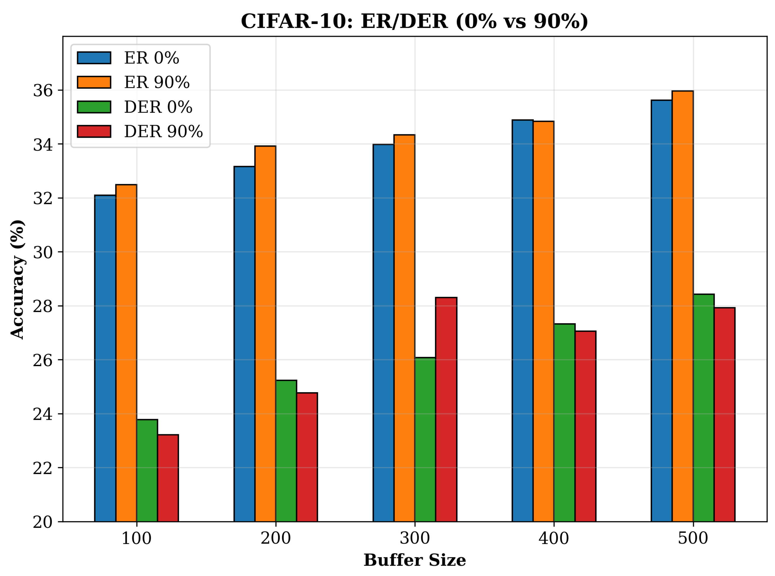
| CIFAR-10 | ER | 0 | 34.16 ± 0.89 | 34.07 ± 0.53 | 33.90 ± 0.62 | 33.59 ± 0.79 | 143.60 ± 2.35 | 220.56 ± 5.42 | 277.41 ± 4.56 | 345.14 ± 9.45 | 6.25 ± 0.09 | 8.20 ± 0.32 | 9.46 ± 0.11 | 11.33 ± 0.04 |
| 25 | 33.93 ± 0.59 | 33.92 ± 0.71 | 33.90 ± 1.06 | 34.15 ± 0.45 | 94.59 ± 0.60 | 140.76 ± 3.76 | 191.74 ± 3.86 | 241.44 ± 2.11 | 4.26 ± 0.06 | 5.52 ± 0.05 | 6.29 ± 0.19 | 7.58 ± 0.07 | ||
| 50 | 34.15 ± 0.77 | 34.27 ± 0.94 | 34.62 ± 0.25 | 34.62 ± 0.49 | 84.83 ± 0.67 | 128.32 ± 1.49 | 164.69 ± 0.71 | 206.37 ± 5.85 | 3.73 ± 0.08 | 4.80 ± 0.12 | 5.62 ± 0.05 | 6.57 ± 0.18 | ||
| 75 | 35.06 ± 0.22 | 34.96 ± 0.74 | 34.83 ± 0.27 | 34.66 ± 0.72 | 75.03 ± 0.90 | 110.29 ± 1.67 | 150.79 ± 4.04 | 182.72 ± 4.75 | 3.29 ± 0.04 | 4.30 ± 0.08 | 4.82 ± 0.07 | 5.37 ± 0.14 | ||
| 90 | 34.36 ± 0.81 | 34.32 ± 0.63 | 34.44 ± 0.68 | 34.40 ± 0.59 | 63.02 ± 0.94 | 96.14 ± 1.15 | 129.04 ± 2.47 | 160.24 ± 1.83 | 2.74 ± 0.00 | 3.68 ± 0.07 | 4.29 ± 0.11 | 4.35 ± 0.07 | ||
| DER | 0 | 26.19 ± 0.02 | 26.29 ± 0.72 | 26.50 ± 1.06 | 26.30 ± 1.15 | 266.88 ± 3.16 | 323.37 ± 5.74 | 399.86 ± 9.45 | 407.72 ± 13.66 | 6.59 ± 0.23 | 8.66 ± 0.08 | 10.52 ± 0.09 | 12.50 ± 0.32 | |
| 25 | 25.48 ± 0.26 | 25.11 ± 0.99 | 25.45 ± 0.66 | 25.69 ± 0.66 | 183.76 ± 1.32 | 217.43 ± 3.68 | 274.12 ± 3.64 | 269.91 ± 4.94 | 4.44 ± 0.07 | 5.79 ± 0.11 | 6.50 ± 0.15 | 8.27 ± 0.23 | ||
| 50 | 26.54 ± 0.27 | 26.88 ± 0.54 | 26.20 ± 0.12 | 26.50 ± 0.40 | 161.27 ± 2.39 | 192.83 ± 1.94 | 243.95 ± 0.94 | 236.41 ± 4.42 | 3.88 ± 0.09 | 5.25 ± 0.05 | 6.06 ± 0.15 | 6.93 ± 0.11 | ||
| 75 | 26.18 ± 0.44 | 25.99 ± 0.22 | 26.68 ± 0.15 | 26.86 ± 0.24 | 140.97 ± 2.22 | 167.29 ± 2.74 | 212.40 ± 3.89 | 211.02 ± 0.48 | 3.39 ± 0.11 | 4.40 ± 0.11 | 5.22 ± 0.07 | 5.85 ± 0.08 | ||
| 90 | 28.40 ± 0.66 | 27.98 ± 0.35 | 28.36 ± 0.13 | 28.53 ± 0.28 | 124.40 ± 1.16 | 145.80 ± 4.29 | 187.15 ± 6.23 | 181.15 ± 6.08 | 2.68 ± 0.06 | 3.56 ± 0.12 | 4.39 ± 0.07 | 4.68 ± 0.05 | ||
| Co2L | 0 | 26.59 ± 0.02 | 26.69 ± 0.75 | 26.90 ± 1.03 | 26.70 ± 1.06 | 269.88 ± 3.21 | 326.37 ± 5.46 | 402.86 ± 9.90 | 410.72 ± 13.42 | 9.59 ± 0.23 | 11.66 ± 0.08 | 13.52 ± 0.09 | 15.50 ± 0.35 | |
| 25 | 25.88 ± 0.24 | 25.51 ± 1.06 | 25.85 ± 0.62 | 26.09 ± 0.60 | 186.76 ± 1.32 | 220.43 ± 3.53 | 277.12 ± 4.00 | 272.91 ± 5.37 | 7.44 ± 0.07 | 8.79 ± 0.10 | 9.50 ± 0.14 | 11.27 ± 0.22 | ||
| 50 | 28.80 ± 0.65 | 28.38 ± 0.34 | 28.76 ± 0.13 | 28.93 ± 0.30 | 164.27 ± 2.23 | 195.83 ± 1.75 | 246.95 ± 0.99 | 239.41 ± 4.23 | 6.88 ± 0.09 | 8.25 ± 0.05 | 9.06 ± 0.16 | 9.93 ± 0.12 | ||
| 75 | 26.58 ± 0.45 | 26.39 ± 0.21 | 27.08 ± 0.16 | 27.26 ± 0.25 | 143.97 ± 2.09 | 170.29 ± 2.63 | 215.40 ± 3.74 | 214.02 ± 0.49 | 6.39 ± 0.10 | 7.40 ± 0.11 | 8.22 ± 0.07 | 8.85 ± 0.09 | ||
| 90 | 26.94 ± 0.29 | 27.28 ± 0.53 | 26.60 ± 0.12 | 26.90 ± 0.38 | 127.40 ± 1.26 | 148.80 ± 3.90 | 190.15 ± 6.16 | 184.15 ± 5.74 | 5.68 ± 0.06 | 6.56 ± 0.11 | 7.39 ± 0.06 | 7.68 ± 0.05 | ||
| CBA | 0 | 26.79 ± 0.02 | 26.89 ± 0.74 | 27.10 ± 0.96 | 26.90 ± 1.04 | 271.88 ± 3.40 | 328.37 ± 5.60 | 404.86 ± 8.68 | 412.72 ± 13.98 | 11.59 ± 0.21 | 13.66 ± 0.07 | 15.52 ± 0.09 | 17.50 ± 0.34 | |
| 25 | 26.08 ± 0.25 | 25.71 ± 1.08 | 26.05 ± 0.61 | 26.29 ± 0.62 | 188.76 ± 1.19 | 222.43 ± 3.92 | 279.12 ± 3.71 | 274.91 ± 5.12 | 9.44 ± 0.07 | 10.79 ± 0.10 | 11.50 ± 0.14 | 13.27 ± 0.21 | ||
| 50 | 27.14 ± 0.29 | 27.48 ± 0.57 | 26.80 ± 0.12 | 27.10 ± 0.44 | 166.27 ± 2.20 | 197.83 ± 1.93 | 248.95 ± 1.02 | 241.41 ± 4.58 | 8.88 ± 0.09 | 10.25 ± 0.05 | 11.06 ± 0.14 | 11.93 ± 0.12 | ||
| 75 | 29.00 ± 0.62 | 28.58 ± 0.38 | 28.96 ± 0.13 | 29.13 ± 0.29 | 145.97 ± 2.17 | 172.29 ± 2.74 | 217.40 ± 3.67 | 216.02 ± 0.46 | 8.39 ± 0.10 | 9.40 ± 0.10 | 10.22 ± 0.07 | 10.85 ± 0.08 | ||
| 90 | 26.78 ± 0.43 | 26.59 ± 0.23 | 27.28 ± 0.15 | 27.46 ± 0.24 | 129.40 ± 1.13 | 150.80 ± 3.95 | 192.15 ± 6.29 | 186.15 ± 5.91 | 7.68 ± 0.06 | 8.56 ± 0.12 | 9.39 ± 0.08 | 9.68 ± 0.05 | ||
| SIESTA | 0 | 26.49 ± 0.02 | 26.59 ± 0.69 | 26.80 ± 1.11 | 26.60 ± 1.10 | 256.88 ± 3.27 | 313.37 ± 6.13 | 389.86 ± 8.51 | 397.72 ± 14.53 | 3.41 ± 0.24 | 1.34 ± 0.09 | 0.52 ± 0.10 | 2.50 ± 0.33 | |
| 25 | 25.78 ± 0.24 | 25.41 ± 0.91 | 25.75 ± 0.68 | 25.99 ± 0.71 | 173.76 ± 1.26 | 207.43 ± 3.83 | 264.12 ± 3.88 | 259.91 ± 4.51 | 5.56 ± 0.07 | 4.21 ± 0.10 | 3.50 ± 0.14 | 1.73 ± 0.24 | ||
| 50 | 28.70 ± 0.61 | 28.28 ± 0.34 | 28.66 ± 0.14 | 28.83 ± 0.27 | 151.27 ± 2.30 | 182.83 ± 2.07 | 233.95 ± 1.00 | 226.41 ± 4.58 | 6.12 ± 0.09 | 4.75 ± 0.05 | 3.94 ± 0.14 | 3.07 ± 0.11 | ||
| 75 | 26.48 ± 0.40 | 26.29 ± 0.20 | 26.98 ± 0.16 | 27.16 ± 0.24 | 130.97 ± 2.13 | 157.29 ± 2.85 | 202.40 ± 3.55 | 201.02 ± 0.48 | 6.61 ± 0.10 | 5.60 ± 0.11 | 4.78 ± 0.07 | 4.15 ± 0.08 | ||
| 90 | 26.84 ± 0.25 | 27.18 ± 0.57 | 26.50 ± 0.11 | 26.80 ± 0.41 | 114.40 ± 1.27 | 135.80 ± 4.39 | 177.15 ± 6.56 | 171.15 ± 6.62 | 7.32 ± 0.06 | 6.44 ± 0.12 | 5.61 ± 0.07 | 5.32 ± 0.05 | ||
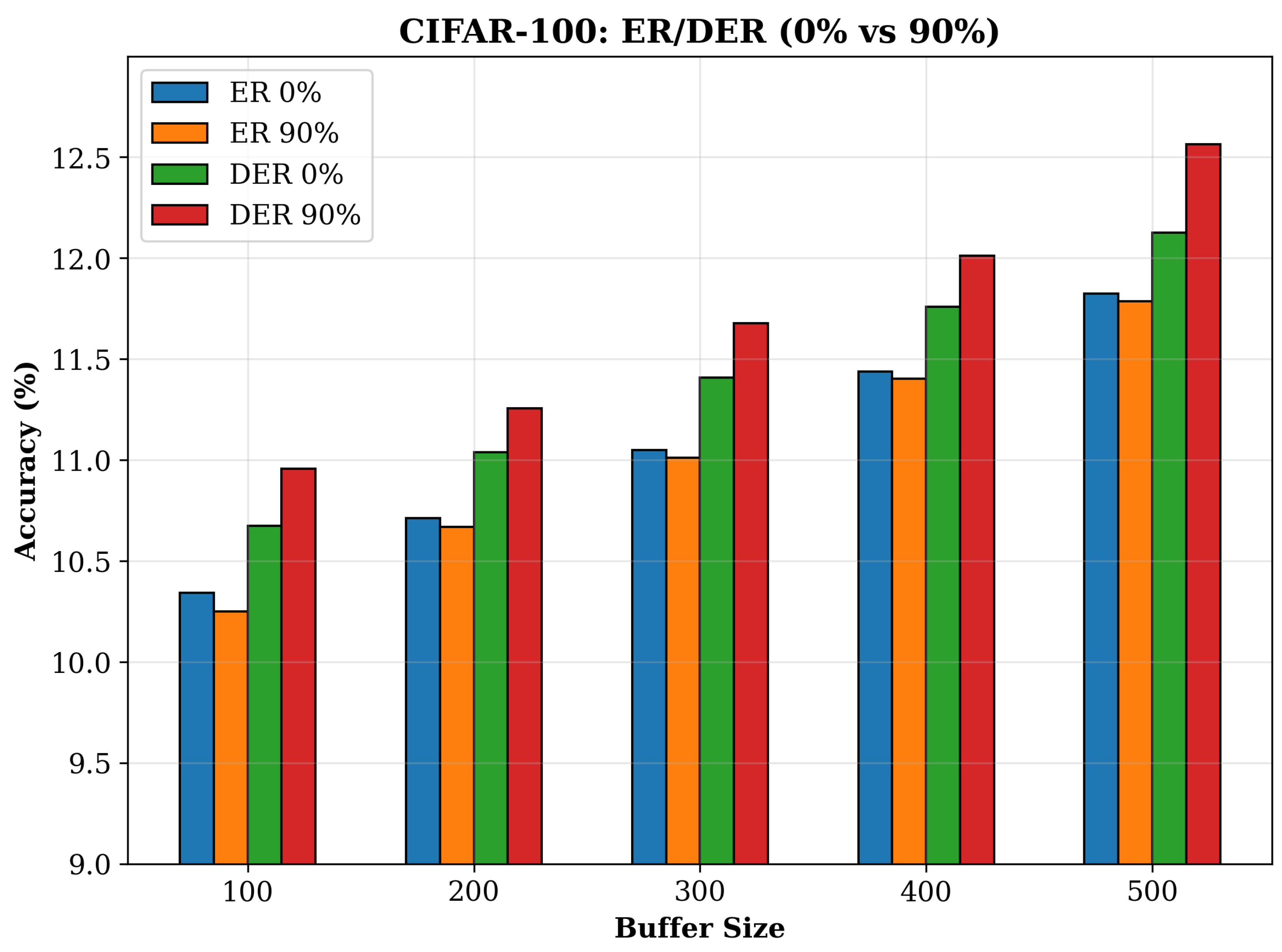
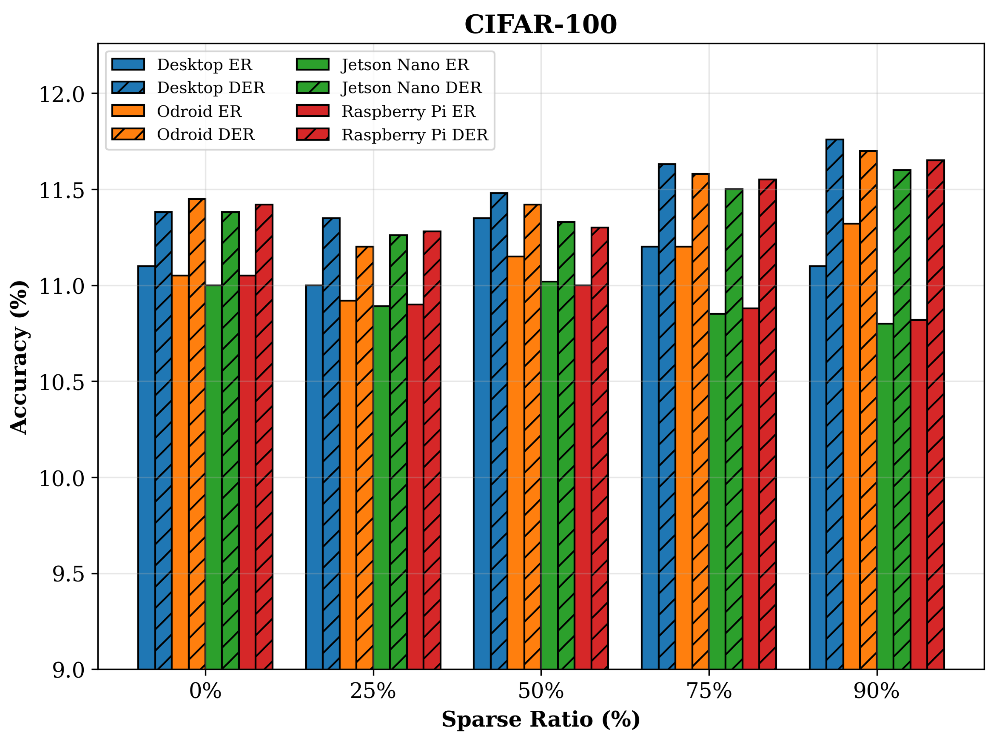
| CIFAR-100 | ER | 0 | 11.11 ± 0.11 | 11.05 ± 0.05 | 10.99 ± 0.25 | 11.29 ± 0.49 | 212.18 ± 3.27 | 310.04 ± 7.39 | 415.86 ± 5.43 | 522.48 ± 8.12 | 8.77 ± 0.08 | 11.40 ± 0.05 | 13.30 ± 0.38 | 16.01 ± 0.20 |
| 25 | 10.91 ± 0.28 | 11.06 ± 0.17 | 10.74 ± 0.20 | 10.95 ± 0.28 | 136.59 ± 5.56 | 204.44 ± 5.56 | 271.30 ± 6.21 | 345.11 ± 6.02 | 6.07 ± 0.08 | 7.85 ± 0.01 | 8.97 ± 0.13 | 11.03 ± 0.24 | ||
| 50 | 11.39 ± 0.09 | 11.10 ± 0.19 | 11.18 ± 0.26 | 10.96 ± 0.10 | 126.14 ± 2.17 | 188.36 ± 2.64 | 252.08 ± 5.49 | 306.42 ± 6.70 | 5.20 ± 0.10 | 6.84 ± 0.02 | 7.75 ± 0.18 | 9.49 ± 0.16 | ||
| 75 | 11.37 ± 0.12 | 11.09 ± 0.05 | 11.08 ± 0.17 | 11.12 ± 0.07 | 113.18 ± 1.80 | 167.47 ± 2.28 | 219.73 ± 3.96 | 280.12 ± 5.94 | 4.53 ± 0.08 | 5.76 ± 0.06 | 6.76 ± 0.16 | 7.72 ± 0.14 | ||
| 90 | 11.15 ± 0.22 | 11.29 ± 0.25 | 10.73 ± 0.39 | 11.03 ± 0.12 | 98.26 ± 1.32 | 146.09 ± 0.90 | 198.31 ± 3.04 | 244.00 ± 0.99 | 3.60 ± 0.08 | 4.80 ± 0.18 | 5.30 ± 0.10 | 6.64 ± 0.21 | ||
| DER | 0 | 11.44 ± 0.11 | 11.31 ± 0.03 | 11.39 ± 0.14 | 11.41 ± 0.17 | 281.76 ± 7.80 | 413.43 ± 10.62 | 560.42 ± 7.66 | 692.27 ± 6.08 | 8.99 ± 0.11 | 11.48 ± 0.24 | 13.30 ± 0.10 | 16.13 ± 0.25 | |
| 25 | 11.29 ± 0.27 | 11.13 ± 0.17 | 11.34 ± 0.04 | 11.31 ± 0.21 | 187.61 ± 5.56 | 281.38 ± 10.59 | 368.16 ± 4.76 | 465.32 ± 15.01 | 6.01 ± 0.16 | 8.07 ± 0.26 | 8.83 ± 0.25 | 10.77 ± 0.17 | ||
| 50 | 11.46 ± 0.21 | 11.50 ± 0.20 | 11.46 ± 0.17 | 11.24 ± 0.30 | 169.31 ± 2.12 | 256.67 ± 10.88 | 332.40 ± 7.17 | 414.51 ± 13.94 | 5.16 ± 0.06 | 6.61 ± 0.09 | 7.67 ± 0.09 | 9.14 ± 0.08 | ||
| 75 | 11.39 ± 0.01 | 11.68 ± 0.29 | 11.57 ± 0.25 | 11.59 ± 0.24 | 150.87 ± 2.81 | 231.50 ± 0.41 | 301.56 ± 6.27 | 377.12 ± 4.36 | 4.35 ± 0.14 | 5.56 ± 0.03 | 6.34 ± 0.07 | 7.60 ± 0.09 | ||
| 90 | 11.85 ± 0.28 | 11.73 ± 0.39 | 11.52 ± 0.14 | 11.83 ± 0.20 | 130.33 ± 1.59 | 198.37 ± 2.87 | 265.34 ± 4.25 | 334.42 ± 6.34 | 3.53 ± 0.02 | 4.36 ± 0.10 | 5.23 ± 0.07 | 6.29 ± 0.11 | ||
| Co2L | 0 | 11.84 ± 0.11 | 11.71 ± 0.03 | 11.79 ± 0.13 | 11.81 ± 0.19 | 284.76 ± 7.67 | 416.43 ± 11.55 | 563.42 ± 7.11 | 695.27 ± 6.39 | 11.99 ± 0.11 | 14.48 ± 0.22 | 16.30 ± 0.10 | 19.13 ± 0.26 | |
| 25 | 12.25 ± 0.29 | 12.13 ± 0.42 | 11.92 ± 0.13 | 12.23 ± 0.22 | 190.61 ± 5.16 | 284.38 ± 11.27 | 371.16 ± 4.77 | 468.32 ± 16.07 | 9.01 ± 0.17 | 11.07 ± 0.26 | 11.83 ± 0.25 | 13.77 ± 0.17 | ||
| 50 | 11.86 ± 0.20 | 11.90 ± 0.20 | 11.86 ± 0.17 | 11.64 ± 0.29 | 172.31 ± 2.03 | 259.67 ± 9.85 | 335.40 ± 7.52 | 417.51 ± 13.93 | 8.16 ± 0.06 | 9.61 ± 0.10 | 10.67 ± 0.10 | 12.14 ± 0.09 | ||
| 75 | 11.79 ± 0.01 | 12.08 ± 0.29 | 11.97 ± 0.25 | 11.99 ± 0.24 | 153.87 ± 3.00 | 234.50 ± 0.37 | 304.56 ± 6.04 | 380.12 ± 4.10 | 7.35 ± 0.13 | 8.56 ± 0.03 | 9.34 ± 0.08 | 10.60 ± 0.09 | ||
| 90 | 11.69 ± 0.28 | 11.53 ± 0.18 | 11.74 ± 0.04 | 11.71 ± 0.19 | 133.33 ± 1.59 | 201.37 ± 2.64 | 268.34 ± 4.57 | 337.42 ± 6.07 | 6.53 ± 0.02 | 7.36 ± 0.11 | 8.23 ± 0.08 | 9.29 ± 0.11 | ||
| CBA | 0 | 12.04 ± 0.10 | 11.91 ± 0.03 | 11.99 ± 0.13 | 12.01 ± 0.16 | 286.76 ± 8.10 | 418.43 ± 11.59 | 565.42 ± 7.78 | 697.27 ± 6.37 | 13.99 ± 0.12 | 16.48 ± 0.25 | 18.30 ± 0.10 | 21.13 ± 0.24 | |
| 25 | 12.45 ± 0.27 | 12.33 ± 0.38 | 12.12 ± 0.13 | 12.43 ± 0.20 | 192.61 ± 5.57 | 286.38 ± 10.48 | 373.16 ± 5.10 | 470.32 ± 14.54 | 11.01 ± 0.16 | 13.07 ± 0.27 | 13.83 ± 0.26 | 15.77 ± 0.16 | ||
| 50 | 12.06 ± 0.21 | 12.10 ± 0.19 | 12.06 ± 0.18 | 11.84 ± 0.31 | 174.31 ± 1.96 | 261.67 ± 11.85 | 337.40 ± 6.67 | 419.51 ± 14.23 | 10.16 ± 0.06 | 11.61 ± 0.08 | 12.67 ± 0.09 | 14.14 ± 0.08 | ||
| 75 | 11.99 ± 0.01 | 12.28 ± 0.29 | 12.17 ± 0.25 | 12.19 ± 0.23 | 155.87 ± 2.72 | 236.50 ± 0.39 | 306.56 ± 6.08 | 382.12 ± 4.74 | 9.35 ± 0.15 | 10.56 ± 0.03 | 11.34 ± 0.08 | 12.60 ± 0.09 | ||
| 90 | 11.89 ± 0.26 | 11.73 ± 0.15 | 11.94 ± 0.04 | 11.91 ± 0.19 | 135.33 ± 1.63 | 203.37 ± 2.63 | 270.34 ± 4.38 | 339.42 ± 6.42 | 8.53 ± 0.02 | 9.36 ± 0.10 | 10.23 ± 0.06 | 11.29 ± 0.10 | ||
| SIESTA | 0 | 11.74 ± 0.11 | 11.61 ± 0.03 | 11.69 ± 0.13 | 11.71 ± 0.16 | 271.76 ± 8.57 | 403.43 ± 9.63 | 550.42 ± 8.11 | 682.27 ± 6.05 | 1.01 ± 0.12 | 1.48 ± 0.23 | 3.30 ± 0.10 | 6.13 ± 0.24 | |
| 25 | 12.15 ± 0.26 | 12.03 ± 0.40 | 11.82 ± 0.13 | 12.13 ± 0.19 | 177.61 ± 5.32 | 271.38 ± 9.93 | 358.16 ± 4.37 | 455.32 ± 15.89 | 3.99 ± 0.17 | 1.93 ± 0.26 | 1.17 ± 0.23 | 0.77 ± 0.17 | ||
| 50 | 11.76 ± 0.21 | 11.80 ± 0.20 | 11.76 ± 0.18 | 11.54 ± 0.27 | 159.31 ± 2.02 | 246.67 ± 11.47 | 322.40 ± 7.19 | 404.51 ± 14.56 | 4.84 ± 0.05 | 3.39 ± 0.09 | 2.33 ± 0.09 | 0.86 ± 0.08 | ||
| 75 | 11.69 ± 0.01 | 11.98 ± 0.27 | 11.87 ± 0.27 | 11.89 ± 0.26 | 140.87 ± 2.92 | 221.50 ± 0.42 | 291.56 ± 6.37 | 367.12 ± 4.53 | 5.65 ± 0.15 | 4.44 ± 0.03 | 3.66 ± 0.06 | 2.40 ± 0.09 | ||
| 90 | 11.59 ± 0.27 | 11.43 ± 0.18 | 11.64 ± 0.04 | 11.61 ± 0.20 | 120.33 ± 1.51 | 188.37 ± 2.79 | 255.34 ± 4.31 | 324.42 ± 6.78 | 6.47 ± 0.02 | 5.64 ± 0.10 | 4.77 ± 0.07 | 3.71 ± 0.11 | ||
| TinyImageNet | ER | 0 | 6.92 ± 0.08 | 6.89 ± 0.08 | 6.91 ± 0.12 | 6.94 ± 0.08 | 368.58 ± 1.92 | 560.85 ± 4.75 | 734.58 ± 8.68 | 920.00 ± 25.85 | 12.63 ± 0.16 | 16.01 ± 0.57 | 18.43 ± 0.49 | 23.45 ± 0.55 |
| 25 | 6.49 ± 0.12 | 6.41 ± 0.08 | 6.44 ± 0.09 | 6.44 ± 0.06 | 247.77 ± 6.69 | 360.69 ± 7.37 | 490.32 ± 9.67 | 603.97 ± 13.01 | 8.31 ± 0.17 | 10.46 ± 0.18 | 12.40 ± 0.29 | 16.09 ± 0.21 | ||
| 50 | 6.93 ± 0.12 | 6.89 ± 0.10 | 6.93 ± 0.05 | 6.93 ± 0.06 | 212.01 ± 1.89 | 318.21 ± 5.36 | 427.68 ± 15.29 | 539.62 ± 8.98 | 6.93 ± 0.20 | 9.12 ± 0.20 | 10.56 ± 0.25 | 13.79 ± 0.45 | ||
| 75 | 6.79 ± 0.03 | 6.81 ± 0.30 | 6.89 ± 0.06 | 6.82 ± 0.03 | 185.48 ± 5.41 | 278.35 ± 7.84 | 364.66 ± 2.60 | 451.95 ± 1.20 | 5.94 ± 0.06 | 7.89 ± 0.14 | 8.87 ± 0.01 | 11.32 ± 0.22 | ||
| 90 | 6.75 ± 0.08 | 6.66 ± 0.07 | 6.73 ± 0.08 | 6.67 ± 0.16 | 153.87 ± 2.00 | 229.73 ± 5.52 | 308.68 ± 6.37 | 383.67 ± 5.69 | 4.74 ± 0.04 | 6.12 ± 0.02 | 7.10 ± 0.17 | 9.08 ± 0.25 | ||
| DER | 0 | 7.13 ± 0.08 | 7.16 ± 0.16 | 7.30 ± 0.01 | 7.07 ± 0.12 | 490.20 ± 10.30 | 734.73 ± 22.86 | 956.09 ± 3.85 | 1256.71 ± 26.78 | 14.00 ± 0.17 | 17.96 ± 0.29 | 21.14 ± 0.57 | 25.25 ± 0.48 | |
| 25 | 6.48 ± 0.05 | 6.39 ± 0.12 | 6.44 ± 0.14 | 6.34 ± 0.03 | 329.63 ± 4.67 | 475.95 ± 7.02 | 628.77 ± 1.08 | 796.89 ± 13.51 | 9.13 ± 0.16 | 12.08 ± 0.36 | 15.19 ± 0.09 | 18.83 ± 0.30 | ||
| 50 | 7.14 ± 0.08 | 7.03 ± 0.05 | 6.99 ± 0.08 | 7.03 ± 0.06 | 284.90 ± 1.63 | 423.41 ± 17.97 | 578.76 ± 2.51 | 714.64 ± 19.62 | 7.54 ± 0.16 | 9.57 ± 0.17 | 12.41 ± 0.17 | 14.94 ± 0.39 | ||
| 75 | 7.07 ± 0.11 | 7.02 ± 0.27 | 6.97 ± 0.16 | 7.04 ± 0.12 | 247.87 ± 3.28 | 370.59 ± 6.77 | 489.26 ± 18.68 | 620.21 ± 12.10 | 6.36 ± 0.10 | 8.21 ± 0.30 | 10.43 ± 0.15 | 12.79 ± 0.20 | ||
| 90 | 7.02 ± 0.05 | 7.13 ± 0.11 | 7.12 ± 0.18 | 7.31 ± 0.07 | 216.29 ± 4.89 | 322.42 ± 5.57 | 428.91 ± 5.35 | 535.12 ± 5.66 | 5.23 ± 0.07 | 6.89 ± 0.04 | 8.64 ± 0.08 | 10.15 ± 0.07 | ||
| Co2L | 0 | 7.53 ± 0.08 | 7.56 ± 0.15 | 7.70 ± 0.01 | 7.47 ± 0.12 | 493.20 ± 10.16 | 737.73 ± 24.31 | 959.09 ± 3.95 | 1259.71 ± 24.79 | 17.00 ± 0.16 | 20.96 ± 0.27 | 24.14 ± 0.57 | 28.25 ± 0.51 | |
| 25 | 6.88 ± 0.05 | 6.79 ± 0.11 | 6.84 ± 0.13 | 6.74 ± 0.03 | 332.63 ± 4.75 | 478.95 ± 6.70 | 631.77 ± 1.09 | 799.89 ± 14.70 | 12.13 ± 0.17 | 15.08 ± 0.39 | 18.19 ± 0.09 | 21.83 ± 0.30 | ||
| 50 | 7.54 ± 0.08 | 7.43 ± 0.05 | 7.39 ± 0.07 | 7.43 ± 0.06 | 287.90 ± 1.75 | 426.41 ± 17.14 | 581.76 ± 2.36 | 717.64 ± 19.58 | 10.54 ± 0.17 | 12.57 ± 0.16 | 15.41 ± 0.16 | 17.94 ± 0.43 | ||
| 75 | 7.47 ± 0.11 | 7.42 ± 0.28 | 7.37 ± 0.17 | 7.44 ± 0.11 | 250.87 ± 3.51 | 373.59 ± 6.79 | 492.26 ± 20.54 | 623.21 ± 12.59 | 9.36 ± 0.09 | 11.21 ± 0.31 | 13.43 ± 0.16 | 15.79 ± 0.19 | ||
| 90 | 7.42 ± 0.05 | 7.53 ± 0.12 | 7.52 ± 0.17 | 7.71 ± 0.07 | 219.29 ± 5.17 | 325.42 ± 6.01 | 431.91 ± 5.88 | 538.12 ± 5.14 | 8.23 ± 0.08 | 9.89 ± 0.04 | 11.64 ± 0.08 | 13.15 ± 0.07 | ||
| CBA | 0 | 7.73 ± 0.07 | 7.76 ± 0.15 | 7.90 ± 0.01 | 7.67 ± 0.13 | 495.20 ± 9.36 | 739.73 ± 23.27 | 961.09 ± 4.04 | 1261.71 ± 26.85 | 19.00 ± 0.17 | 22.96 ± 0.29 | 26.14 ± 0.55 | 30.25 ± 0.50 | |
| 25 | 7.08 ± 0.05 | 6.99 ± 0.11 | 7.04 ± 0.13 | 6.94 ± 0.03 | 334.63 ± 4.25 | 480.95 ± 6.37 | 633.77 ± 1.18 | 801.89 ± 14.31 | 14.13 ± 0.18 | 17.08 ± 0.37 | 20.19 ± 0.09 | 23.83 ± 0.27 | ||
| 50 | 7.74 ± 0.08 | 7.63 ± 0.05 | 7.59 ± 0.07 | 7.63 ± 0.06 | 289.90 ± 1.47 | 428.41 ± 18.50 | 583.76 ± 2.32 | 719.64 ± 18.99 | 12.54 ± 0.17 | 14.57 ± 0.16 | 17.41 ± 0.18 | 19.94 ± 0.42 | ||
| 75 | 7.67 ± 0.11 | 7.62 ± 0.25 | 7.57 ± 0.16 | 7.64 ± 0.11 | 252.87 ± 3.01 | 375.59 ± 6.98 | 494.26 ± 18.30 | 625.21 ± 11.21 | 11.36 ± 0.09 | 13.21 ± 0.32 | 15.43 ± 0.14 | 17.79 ± 0.19 | ||
| 90 | 7.62 ± 0.05 | 7.73 ± 0.11 | 7.72 ± 0.18 | 7.91 ± 0.06 | 221.29 ± 4.41 | 327.42 ± 5.77 | 433.91 ± 5.69 | 540.12 ± 5.94 | 10.23 ± 0.07 | 11.89 ± 0.04 | 13.64 ± 0.08 | 15.15 ± 0.07 | ||
| SIESTA | 0 | 7.43 ± 0.08 | 7.46 ± 0.17 | 7.60 ± 0.01 | 7.37 ± 0.12 | 480.20 ± 11.08 | 724.73 ± 20.84 | 946.09 ± 3.74 | 1246.71 ± 24.97 | 4.00 ± 0.16 | 7.96 ± 0.27 | 11.14 ± 0.56 | 15.25 ± 0.49 | |
| 25 | 6.78 ± 0.05 | 6.69 ± 0.11 | 6.74 ± 0.15 | 6.64 ± 0.03 | 319.63 ± 4.91 | 465.95 ± 7.39 | 618.77 ± 1.17 | 786.89 ± 13.24 | 0.87 ± 0.15 | 2.08 ± 0.34 | 5.19 ± 0.09 | 8.83 ± 0.29 | ||
| 50 | 7.44 ± 0.08 | 7.33 ± 0.05 | 7.29 ± 0.08 | 7.33 ± 0.06 | 274.90 ± 1.63 | 413.41 ± 17.65 | 568.76 ± 2.38 | 704.64 ± 18.07 | 2.46 ± 0.17 | 0.43 ± 0.18 | 2.41 ± 0.17 | 4.94 ± 0.42 | ||
| 75 | 7.37 ± 0.10 | 7.32 ± 0.29 | 7.27 ± 0.15 | 7.34 ± 0.12 | 237.87 ± 3.06 | 360.59 ± 7.15 | 479.26 ± 17.29 | 610.21 ± 11.88 | 3.64 ± 0.10 | 1.79 ± 0.33 | 0.43 ± 0.16 | 2.79 ± 0.21 | ||
| 90 | 7.32 ± 0.05 | 7.43 ± 0.11 | 7.42 ± 0.20 | 7.61 ± 0.07 | 206.29 ± 5.17 | 312.42 ± 5.06 | 418.91 ± 5.51 | 525.12 ± 5.28 | 4.77 ± 0.07 | 3.11 ± 0.04 | 1.36 ± 0.07 | 0.15 ± 0.07 | ||
Disclaimer/Publisher’s Note: The statements, opinions and data contained in all publications are solely those of the individual author(s) and contributor(s) and not of MDPI and/or the editor(s). MDPI and/or the editor(s) disclaim responsibility for any injury to people or property resulting from any ideas, methods, instructions or products referred to in the content. |
© 2025 by the authors. Licensee MDPI, Basel, Switzerland. This article is an open access article distributed under the terms and conditions of the Creative Commons Attribution (CC BY) license (https://creativecommons.org/licenses/by/4.0/).
Share and Cite
Park, H.-S.; Chu, H.-C.; Sung, M.-K.; Kim, C.; Lee, J.; Kim, D.-W.; Lee, J. Survey on Replay-Based Continual Learning and Empirical Validation on Feasibility in Diverse Edge Devices Using a Representative Method. Mathematics 2025, 13, 2257. https://doi.org/10.3390/math13142257
Park H-S, Chu H-C, Sung M-K, Kim C, Lee J, Kim D-W, Lee J. Survey on Replay-Based Continual Learning and Empirical Validation on Feasibility in Diverse Edge Devices Using a Representative Method. Mathematics. 2025; 13(14):2257. https://doi.org/10.3390/math13142257
Chicago/Turabian StylePark, Heon-Sung, Hyeon-Chang Chu, Min-Kyung Sung, Chaewoon Kim, Jeongwon Lee, Dae-Won Kim, and Jaesung Lee. 2025. "Survey on Replay-Based Continual Learning and Empirical Validation on Feasibility in Diverse Edge Devices Using a Representative Method" Mathematics 13, no. 14: 2257. https://doi.org/10.3390/math13142257
APA StylePark, H.-S., Chu, H.-C., Sung, M.-K., Kim, C., Lee, J., Kim, D.-W., & Lee, J. (2025). Survey on Replay-Based Continual Learning and Empirical Validation on Feasibility in Diverse Edge Devices Using a Representative Method. Mathematics, 13(14), 2257. https://doi.org/10.3390/math13142257