Abstract
Unknown time-varying parameters, along with mismatched and matched disturbances, exist in hydraulic systems, worsening position tracking performance and even destabilizing systems. To address this issue, this article proposes an adaptive full-state prescribed performance position tracking control for hydraulic systems subject both to unknown time-varying parameters and to mismatched and matched disturbances. First, a smooth nonlinear term is skillfully introduced into the controller design so that it can simultaneously cope with both unknown time-varying parameters and disturbances. Next, by integrating the adaptive technique and the prescribed performance function, an adaptive full-state prescribed performance position tracking controller is developed for hydraulic systems in which both the transient and steady performance of all the control errors can be prescribed. A stability analysis then confirms both the prescribed transient performance and the asymptotic steady performance of all the control errors. Finally, the superiority of the proposed controller is also validated by comparison with simulation results.
Keywords:
hydraulic system; position tracking; time-varying parameters and disturbances; prescribed performance; adaptive technique MSC:
76A02; 93C10; 93C40; 93D21
1. Introduction
Hydraulic systems have long played a role in industrial applications due to their large force/torque output capabilities and small size-to-power ratios [1,2,3,4,5,6,7,8,9,10]. However, the achievement of high-precision tracking control for hydraulic systems is hard because of the existence of both high nonlinearities and large uncertainties. To surmount this problem, many controls have been developed for hydraulic systems during recent years. An output-feedback nonlinear robust control was proposed for hydraulic systems in [11], in which an extended state observer (ESO) was adopted to estimate unknown system states and compensate for unknown disturbances. Subsequently, in [12], Na et al. employed a finite-time sliding mode state observer and presented a novel unknown system dynamics estimator-based control method for hydraulic systems, confirming the validity of their approach through extensive experimental results. In [13], Ba et al. developed a sliding mode observer (SMO) that was designed to compensate for unknown dynamics in hydraulic systems. Excellent zero-error control performance was also found to hold theoretically in [13]. However, the assumption that the boundedness of the second-order derivatives of disturbances must be met might have limited the actual application of SMO in [13]. Remarkably, the designs of all the above controllers neglected to account for the large parametric uncertainties which result from component wear and temperature change in hydraulic systems, the existence of which can worsen control performance and even cause systems to be destabilized.
To improve robustness against both unknown disturbances and parametric uncertainties and, furthermore, to achieve expected control performance, a typical control framework named adaptive robust control was developed in [14] and subsequently successfully utilized in hydraulic systems [15,16,17,18,19]. In [20], Wang et al. exploited an ESO-based nonlinear adaptive control method for single-rod hydraulic systems, and obtained experimental results which confirmed the merits of the proposed approach. A two-ESO-based adaptive robust control method was exploited for hydraulic systems in [21], in which ESOs were utilized to estimate both the unmeasured velocity value and unknown disturbances. An output-feedback-based adaptive-gain super-twisting sliding mode control framework was exploited for hydraulic systems in [22], in which the ESO was utilized to estimate the unknown system states and disturbances. However, the adaptive controllers reported in [11,12,13,14,15,16,17,18,19,20,21,22] only obtained bounded-error tracking performance in theory. Moreover, these adaptive controllers always assumed that unknown parameters existing in hydraulic systems were constant. However, temperature change and component wear, both unknown time-varying parameters and disturbances, exist widely in hydraulic systems. The problem of how to cope with both unknown time-varying parameters and time-varying disturbances is still, then, a challenge for hydraulic systems.
The other motivation for this paper is that all the aforementioned controllers were designed to achieve enhancement of steady performance in hydraulic systems while ignoring transient performance. To meet the requirements of prescribed transient performance for hydraulic systems, Xu et al. combined ESO and a prescribed performance function (PPF) in [23,24,25], then overcame the problem of motion control for state-constrained hydraulic systems in [26], in which the constraints of all system states could not be violated and tracking performance could always be kept in a prescribed region using their proposed controller. The authors of [27] used the Barrier Lyapunov Function and the PPF to develop an output feedback-based adaptive prescribed performance controller for hydraulic systems, achieving the prescribed transient performance of the tracking error without the violation of full-state constraints. Guo et al. exploited an adaptive prescribed performance backstepping controller for hydraulic manipulators in [28], in which large coupled uncertainties were estimated and compensated for using a neural network. In contrast, in previous controllers [23,24,25,26,27,28], only the preset performance of the tracking error could be assured, while unknown parameters needed to be assumed to remain time-invariant. The question of how to design an adaptive prescribed performance control method for hydraulic systems with unknown time-varying parameters while obtaining the prescribed performance of all the control errors is therefore still an open one.
Motivated by the above facts, in this study we propose an adaptive full-state prescribed performance position tracking controller for hydraulic systems which delivers both the prescribed transient performance and the asymptotic steady performance of all the control errors. Compared to previous studies which sought to obtain control results for hydraulic systems, the contributions of this paper can be stated as follows:
- (1)
- An adaptive full-state prescribed performance position tracking controller is developed for hydraulic systems, in which both the boundedness of all the closed-loop signals and the asymptotic steady performance of the position tracking error can be ensured.
- (2)
- By skillfully introducing a smooth nonlinear function, unknown time-varying parameters and disturbances are both handled simultaneously, thereby relaxing the assumption that unknown parameters should be constant or their derivatives should be bounded, which underlies existing adaptive control results [11,12,13,14,15,16,17,18,19,20,21,22].
- (3)
- Unlike with existing controllers that can only ensure the prescribed performance of the output error in [23,24,25,26,27,28], both the prescribed transient performance and the steady performance of all the control errors for hydraulic systems are guaranteed.
2. System Modeling
The considered hydraulic system is illustrated in Figure 1, in which it can be seen that the valve-controlled hydraulic axis causes the load to move.
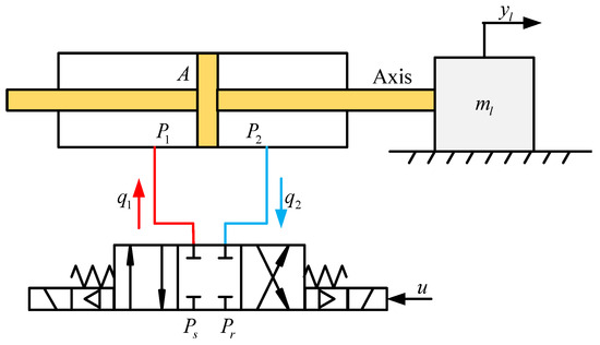
Figure 1.
Schematic diagram of the hydraulic system.
The dynamics of the load can be denoted as
where and denote the load mass and displacement; and denote the pressure values of the two chambers; denotes the effective piston area; () are time-varying parameters that denote the amplitudes of viscous friction, Coulomb friction, and the Stribeck effect, respectively; denotes shape coefficients that approximate Coulomb friction and the Stribeck effect; and denotes the unknown mismatched disturbance.
Following [29], the pressure dynamics of the hydraulic actuator can be denoted as
where and denote the respective volumes of the two chambers, with V01 and V02 standing for the initial respective volumes of the two chambers; is the effective oil bulk modulus; is the time-varying internal leakage coefficient; and denote, respectively, the supplied and return flow rate values; and and denote the unknown uncertainties.
Because a high-performance servo valve is utilized in the considered hydraulic system, the dynamics of the valve can be omitted. Therefore, and following [29], the flow rate values and can be obtained as follows:
where kq is the flow gain, and is
From (2), we get
The following can also be obtained:
where
Using (1) and (6), constructing the variables yields
in which
Uniting (9), and defining the unknown time-varying parameter set , we obtain
in which
Our objective is to design a control input to obtain both the prescribed transient performance and the asymptotic steady performance for hydraulic systems subject to both unknown time-varying parameters and disturbances under Assumption 1, as follows:
Assumption 1.
The reference command meets with . The unknown time-varying parameter set meets with .
3. Adaptive Prescribed Performance Controller Design
3.1. Error Variable Transformation and Prescribed Performance Function Transformation
First, we construct the following error variables:
where () denote the virtual controls; and denote filtered signals of .
To get the filtering signals , a set of nonlinear filters is presented as follows:
in which denote the filtering errors; ; meets , , with a constant ; and .
To achieve the full-state prescribed transient performance of all the control errors, the following performance indexes hold:
with the prescribed performance functions being designed as
where , , and c are positive constants; and .
To promote the subsequent controller design, we define the transformation variables as follows:
3.2. Controller Design
The specific prescribed performance controller design procedure is provided below.
Step 1: Differentiating in (16) yields
Choosing the Lyapunov Function yields
The virtual control is designed as follows:
where and .
Putting (19) into (18), we get
Step 2: Differentiating in (16) yields
Choosing the Lyapunov Function yields
The virtual control is designed as follows:
where and ; denotes the estimate of ; and the term is denoted as
where .
Putting (23) into (22), we get
Step 3: Differentiating in (16) yields
We choose the Lyapunov Function, as follows:
where is composed of the maximum value of each element in the set ; and denotes the adjustable positive parameter adaption matrix.
We therefore obtain the following:
The control input is designed as follows:
where and ; and the term is denoted as
where .
Putting (29) into (28), we get
Defining , accordingly, we get
We construct the following parameter updated law:
where .
The following is now obtained:
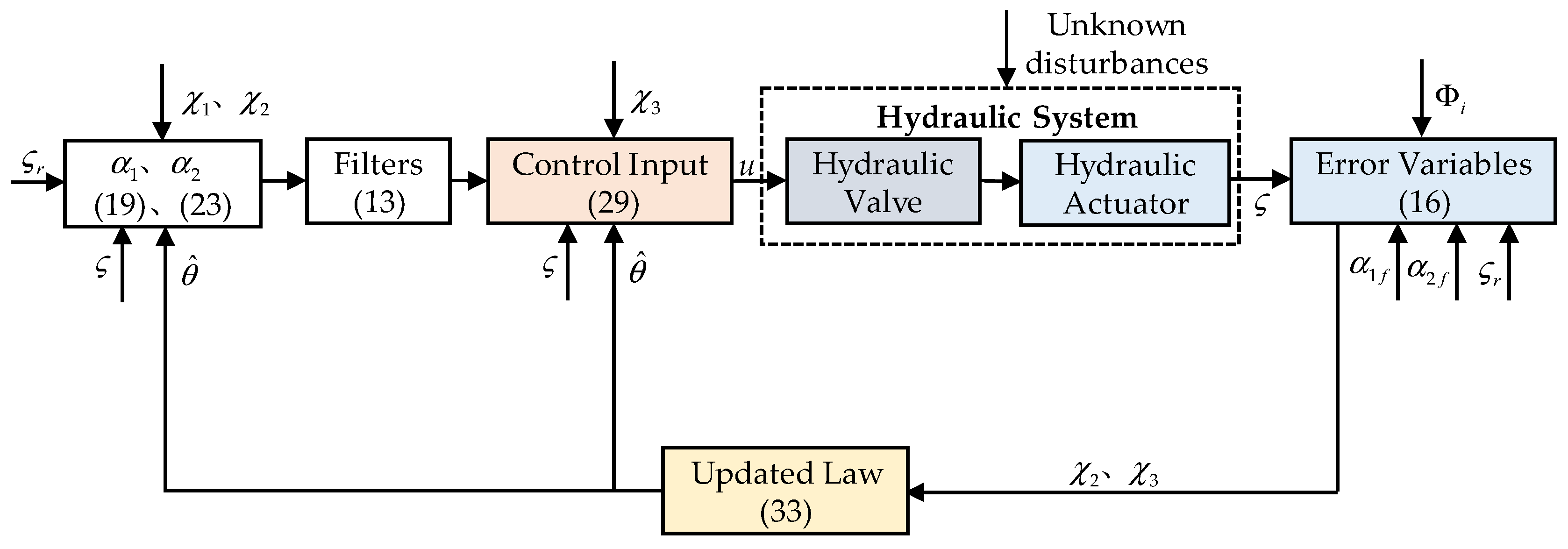
The developed controller diagram of the hydraulic system is presented below (Figure 2).
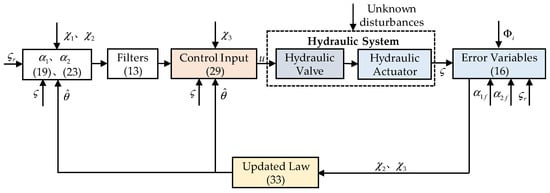
Figure 2.
Controller diagram of the hydraulic system.
3.3. Main Result and Stability Analysis
The main result of this paper is provided below.
Theorem 1.
Under Assumption 1, the control law (29) and the parameter updated law (33), by picking up the proper control parameters , , , , , , and c for and , we determine the following: (1) the boundedness of all the closed-loop signals holds; (2) both the prescribed transient performance and the asymptotic steady performance of all the control errors hold.
Proof of Theorem 1.
We construct a new Lyapunov Function, as follows:
According to (13), (34), and (35), we obtain
We note that
We now obtain
where .
From Assumption 1, the compact set holds. Also, the compact set holds with . Hence, the set is compact. Accordingly, there are positive constants and such that and on .
Hence, we get
The following inequalities hold:
We now obtain
where and .
Integrating the two sides of (41), we get
Hence, the boundedness of all the system signals holds, and is uniformly continuous. Using Barbalat’s lemma [30], as . Thus, all the control errors asymptotically can converge to zero. From (35), one obtains on for . Accordingly, one obtains .
Consequently, Theorem 1 holds. □
4. Simulation Results
In this section, the effectiveness of the designed controller is verified through simulation comparison using the software Matlab/Simulink 2016a. The time-varying parameters of the system are set as , , , and ; the disturbances are set as , , and . The other physical parameters of the hydraulic system are presented in Table 1. The sample time is set to 0.5 ms. The simulation time is set to 40 s.

Table 1.
Physical parameters of the hydraulic system.
Two controllers are compared to validate the effectiveness of the developed controller in the article.
(1) AAPPC: This is the controller proposed in this paper, whose controller parameters are as follows: , , , , , , , , , , , , , , , and . Also, the initial value of the unknown time-varying parameter set is set as .
(2) AAC: This controller is an adaptive controller without prescribed performance functions. The corresponding control parameters of AAC are the same as those of AAPPC. The goal of the comparison with AAC is to validate the effectiveness of full-state prescribed performance functions in AAPPC.
Two simulation cases were run to validate the effectiveness of the controller proposed in this paper.
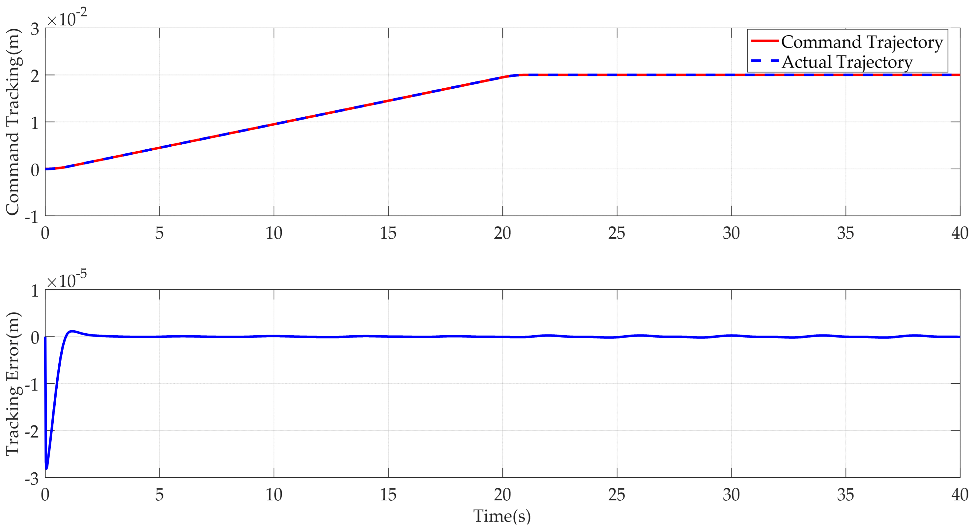
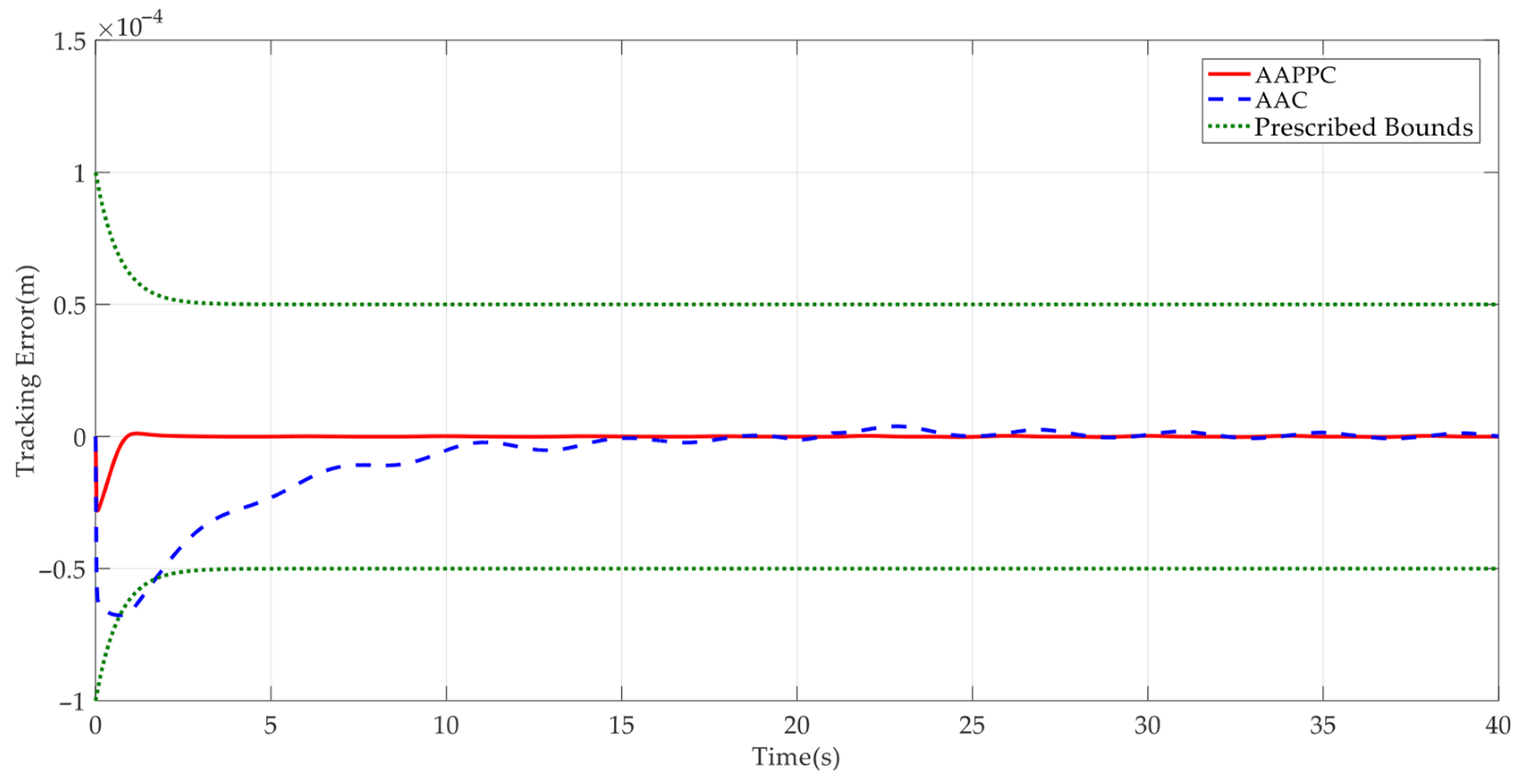
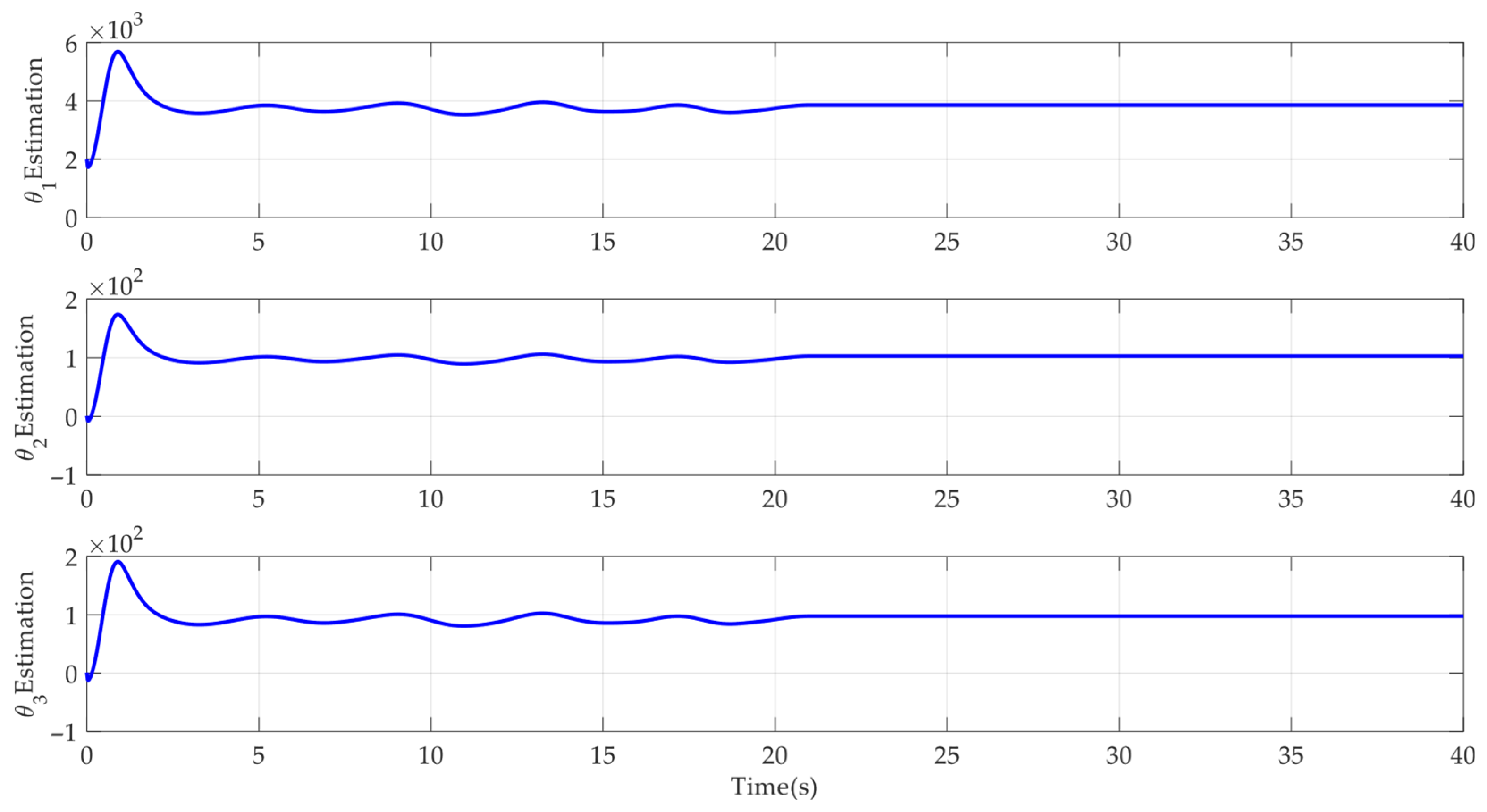
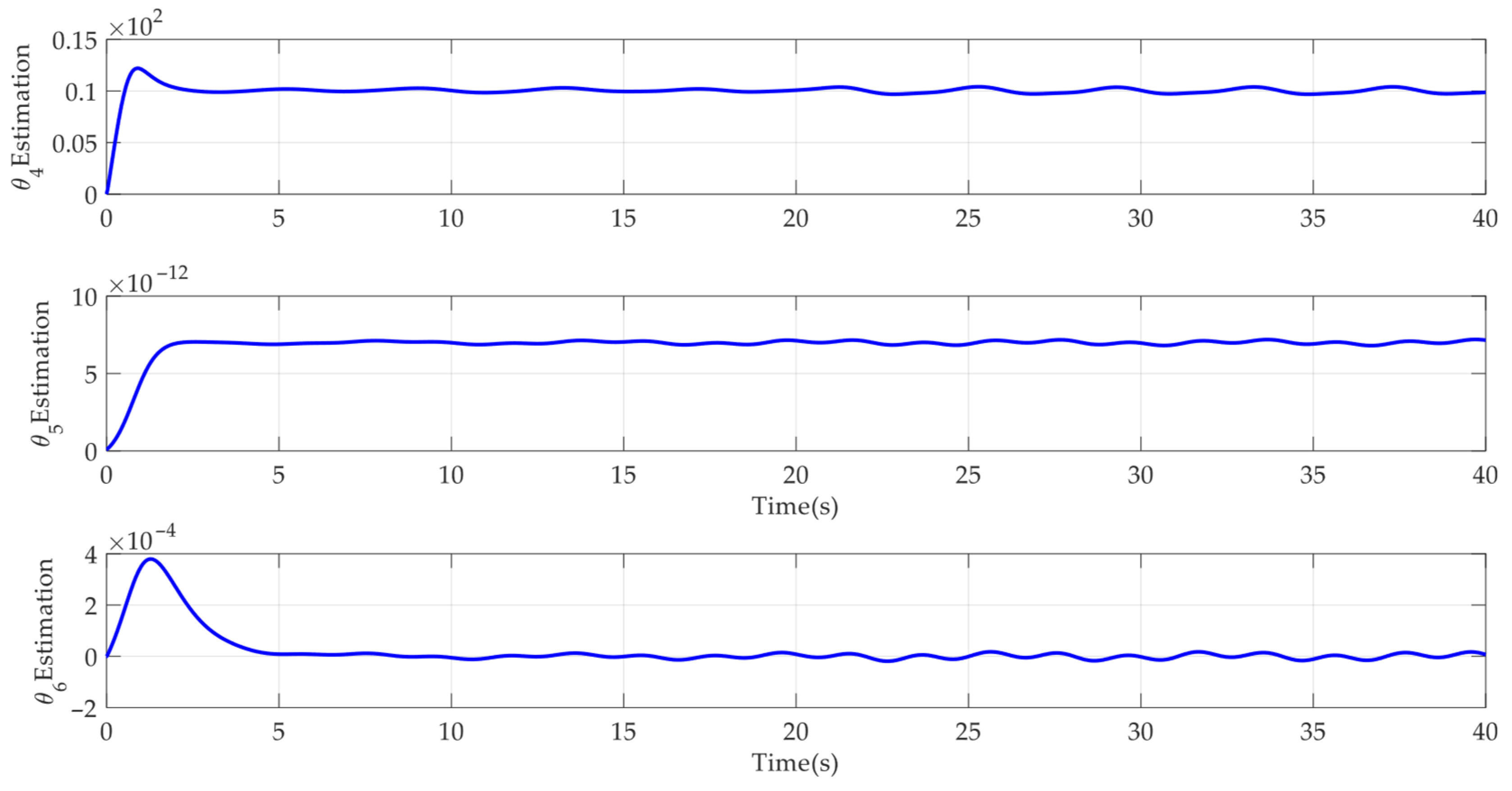
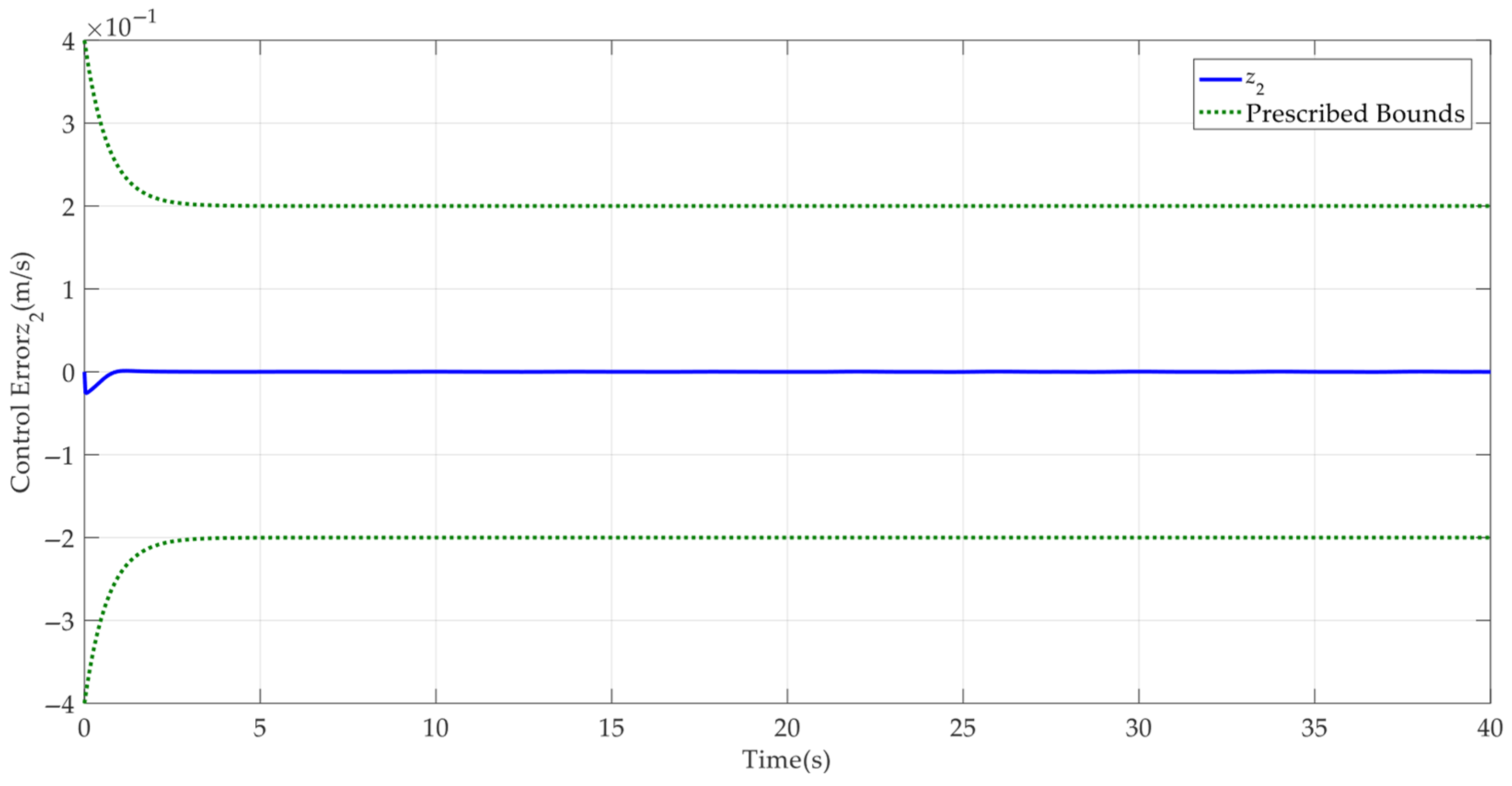
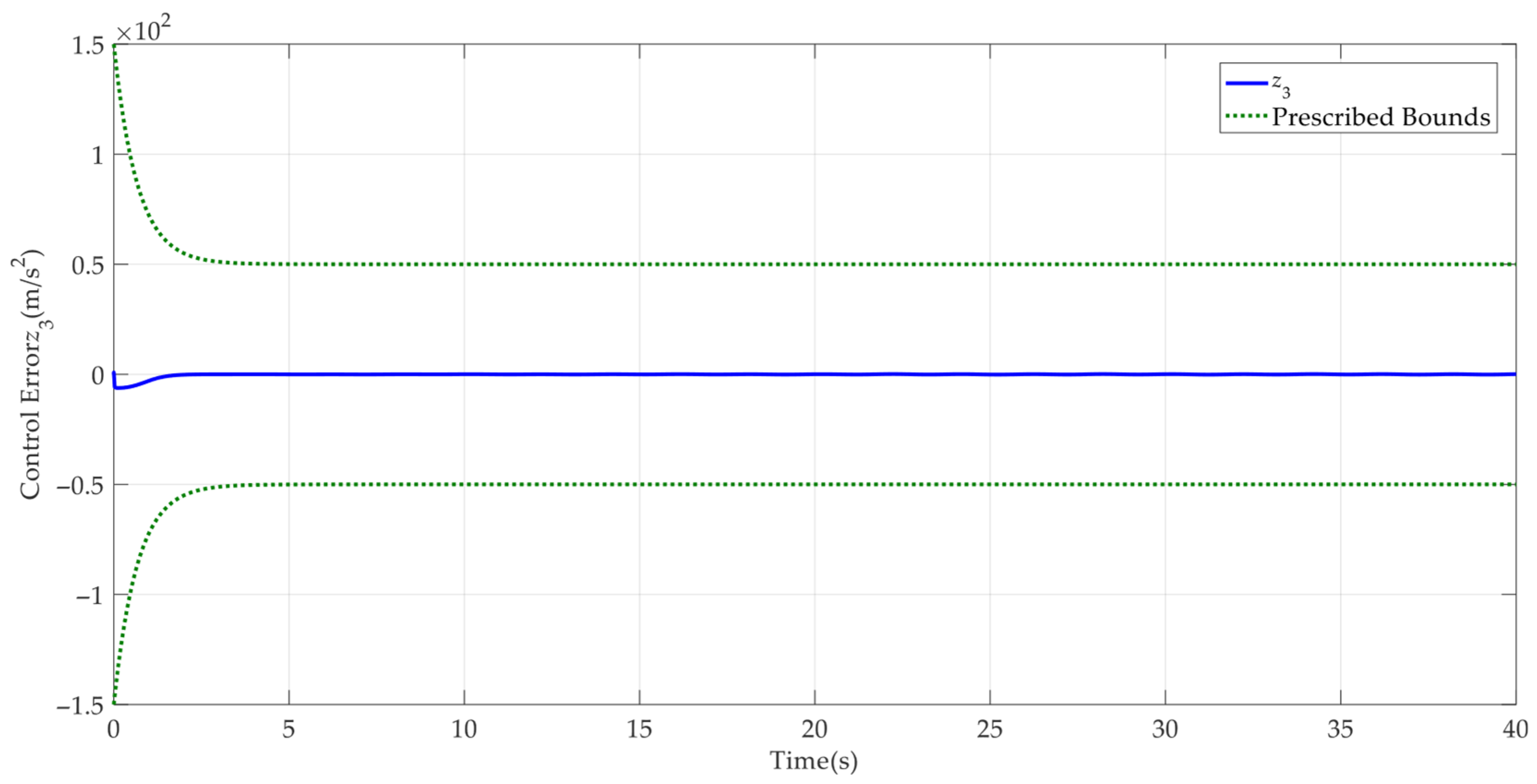
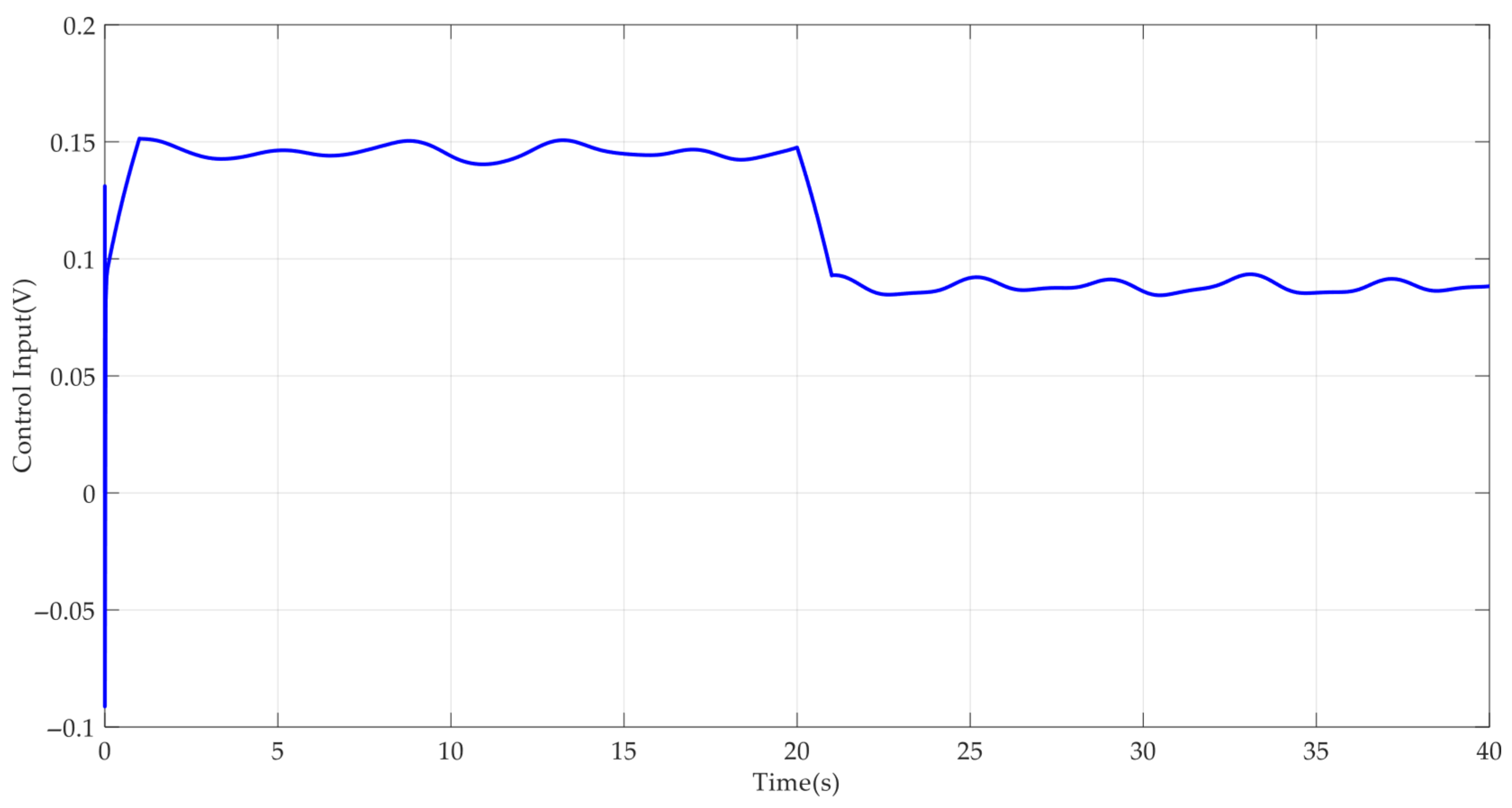
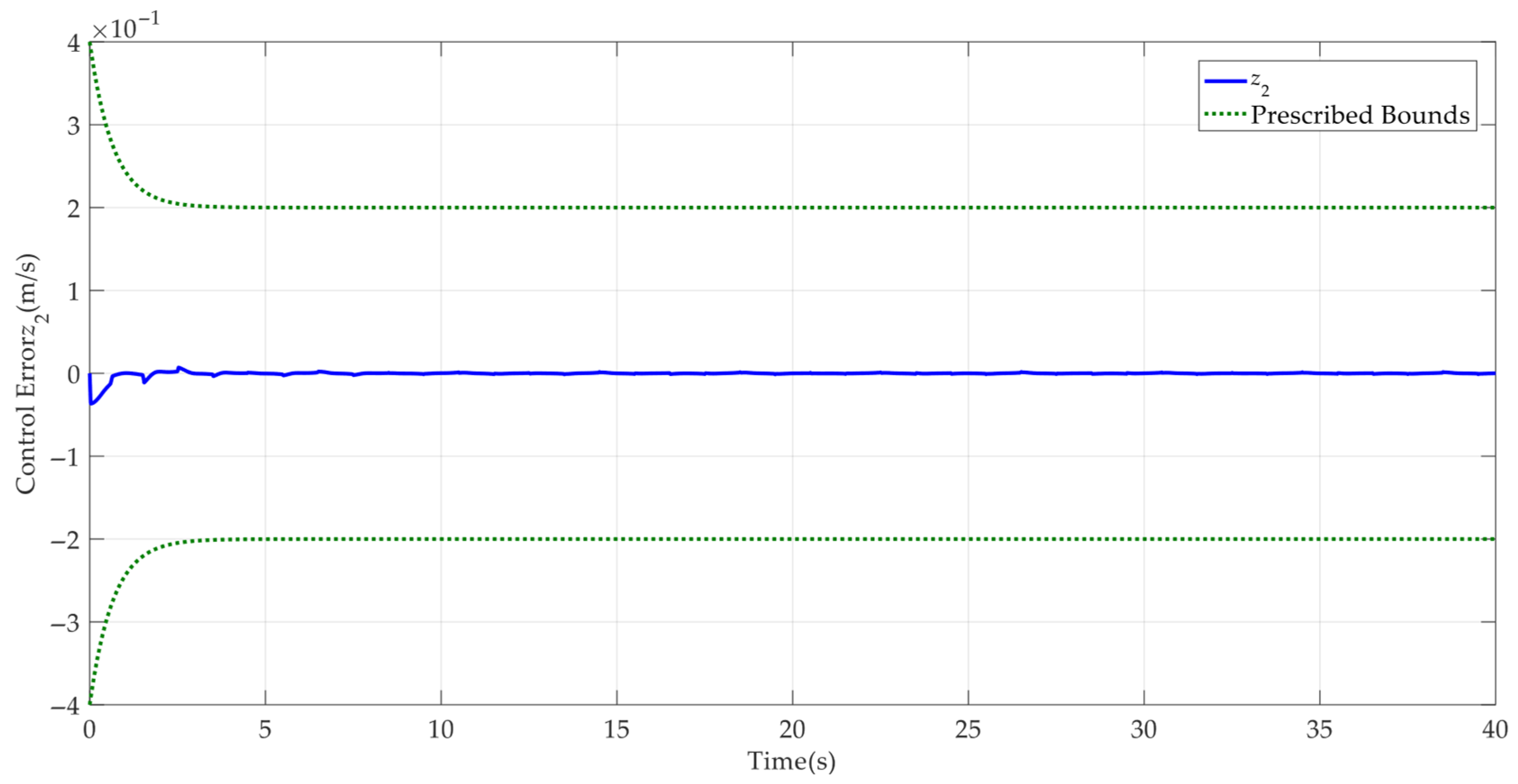
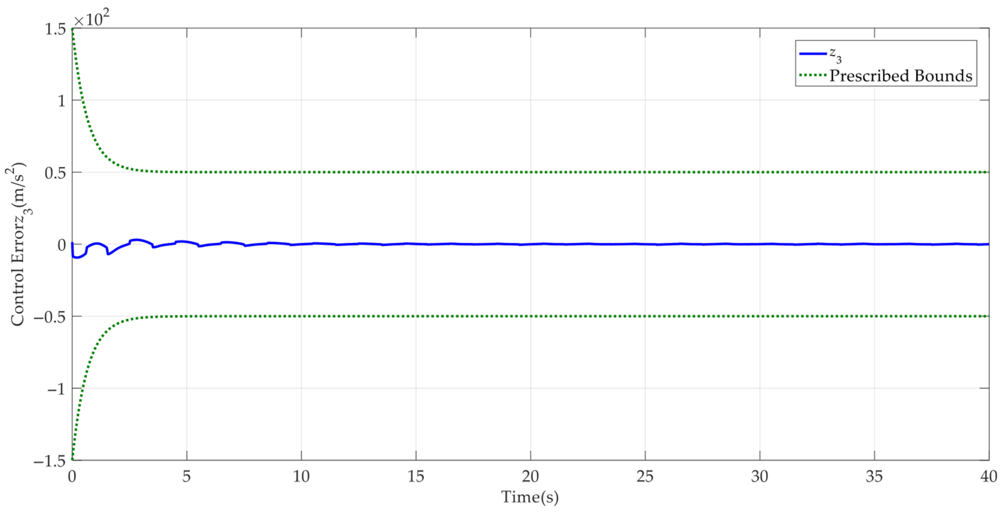
Case 1: First a step-like reference command was employed to test the control performance of the developed control method. The corresponding simulation results are shown in Figure 3, Figure 4, Figure 5, Figure 6, Figure 7, Figure 8 and Figure 9. It can be seen from Figure 3 that the developed AAPPC can achieve excellent asymptotic tracking performance. The curves of tracking errors between AAPPC and AAC are shown in Figure 4, in which it can be seen that the steady-state tracking error of AAPPC controller is approximately 1 × 10⁻³ mm while that of AAC is approximately 2 × 10⁻³ mm. It is also obvious that AAC has good asymptotic tracking performance and steady-state tracking accuracy, owing to the employment of the time-varying parameter adaptive technique in AAPPC. In contrast, when the prescribed performance function is not used to constrain the control errors, the initial transient of its tracking error z1 exceeds the set safety performance bounds in AAC. Furthermore, the tracking error z1 of AAPPC is always within the set safety performance boundary range, which verifies the effectiveness of the prescribed performance mechanism in AAPPC. In addition, it can be seen in Figure 5 and Figure 6 that the estimates of the unknown time-varying parameters and disturbances of the system both have good convergence performance, thereby verifying the effectiveness of the designed parameter adaptive law in AAPPC. The control errors z2 and z3 of AAPPC are shown in Figure 7 and Figure 8, respectively, in which it can be seen that z2 and z3 are always within the set safety performance boundary range. The control input curve in AAPPC is shown in Figure 9. Its amplitude is within ±0.2 V, and it is smooth and continuous, which is conducive to actual application of the controller.
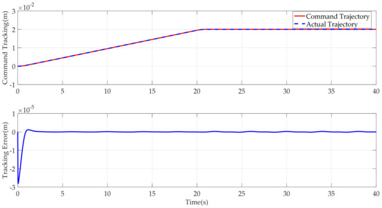
Figure 3.
Tracking performance of AAPPC.
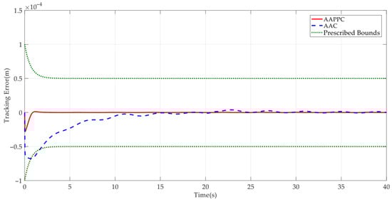
Figure 4.
Tracking errors of compared controllers.
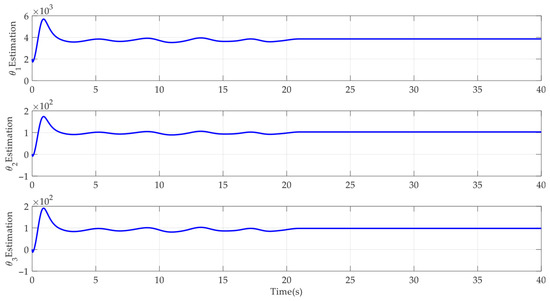
Figure 5.
Estimation of θ1~θ3 in AAPPC.
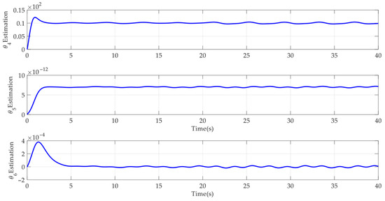
Figure 6.
Estimation of θ4~θ6 in AAPPC.
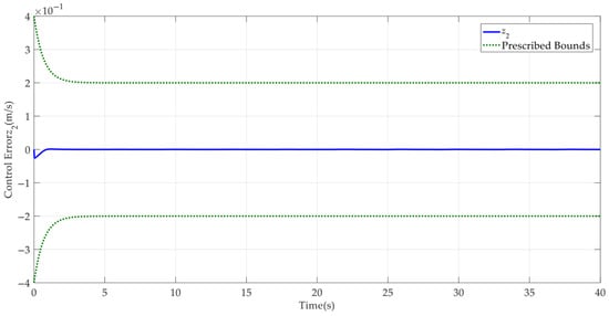
Figure 7.
Control error z2 in AAPPC.
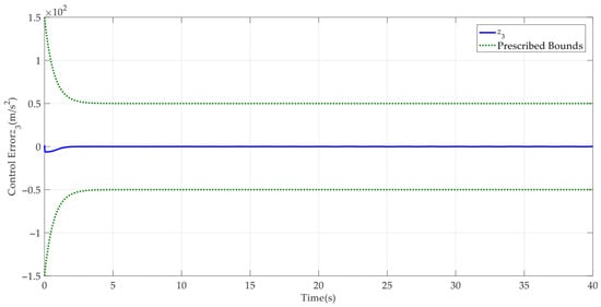
Figure 8.
Control error z3 in AAPPC.
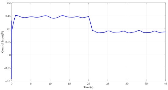
Figure 9.
Control input in AAPPC.
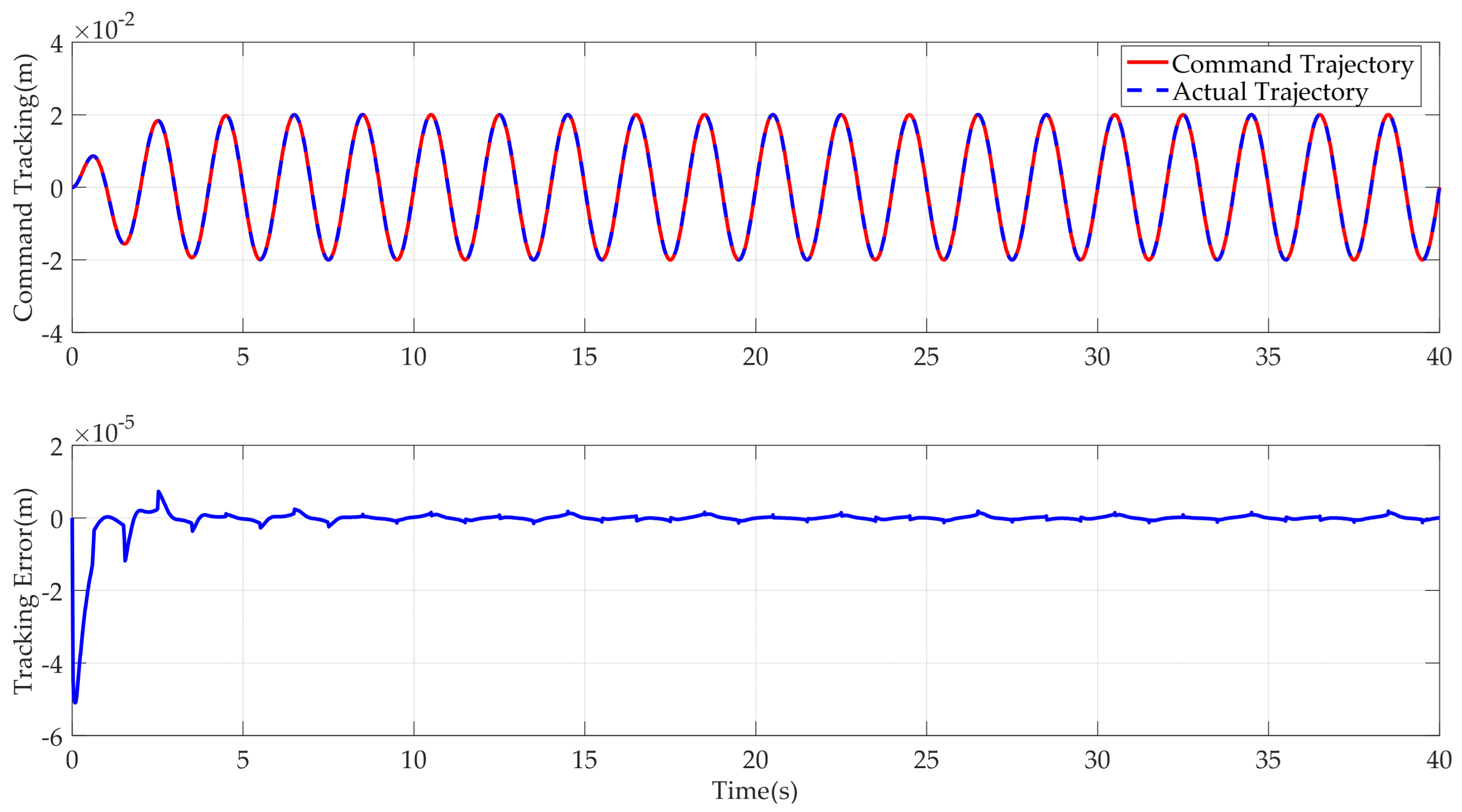
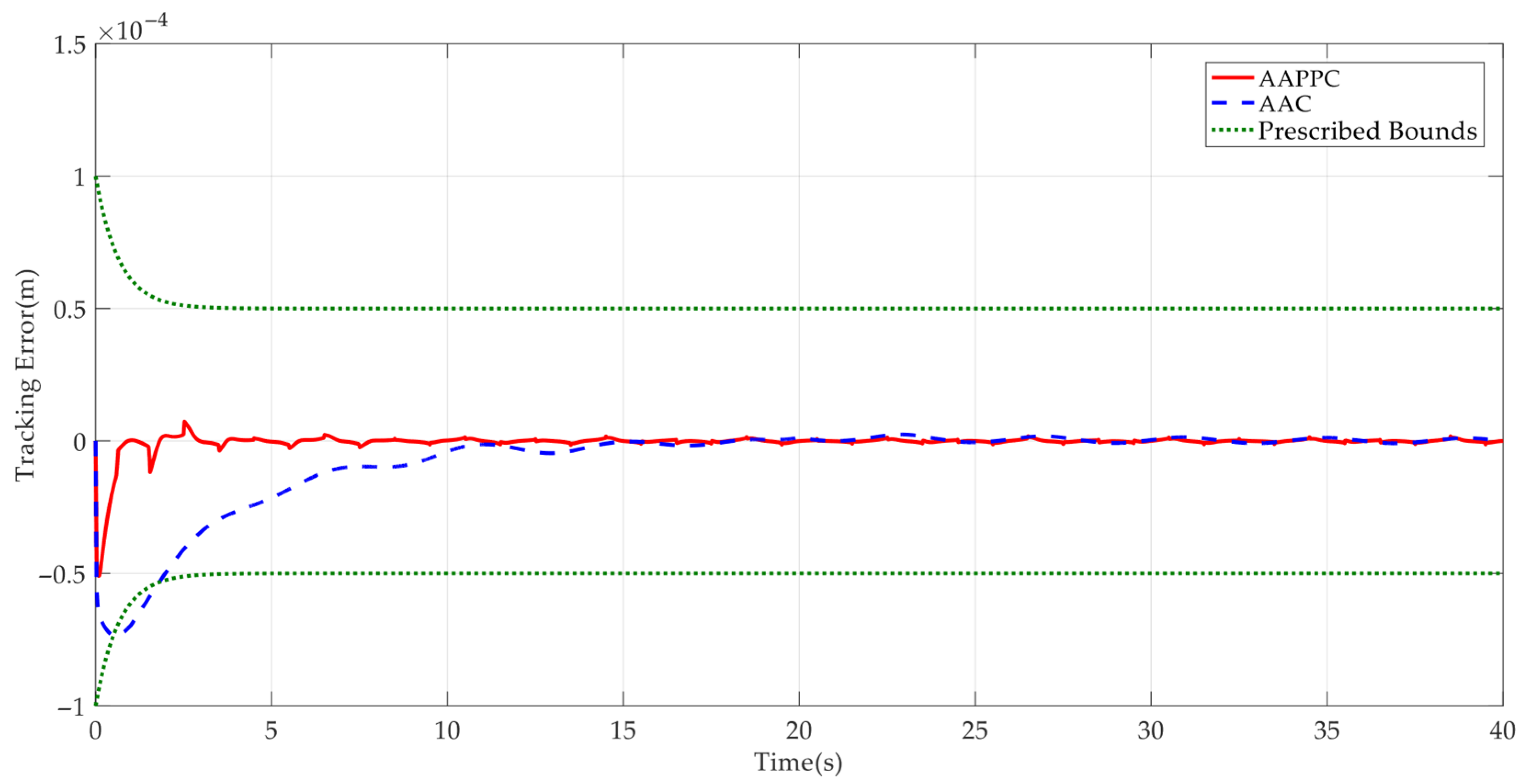
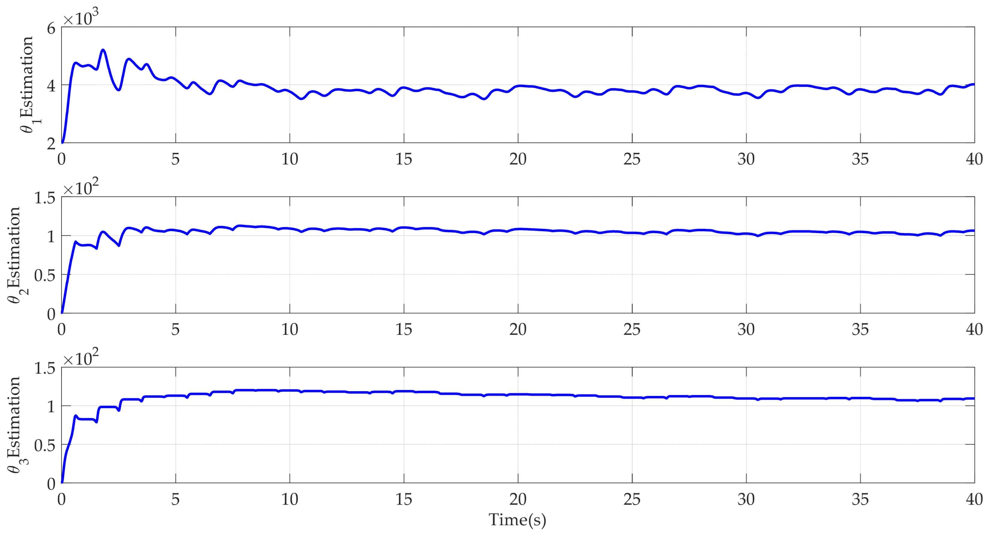
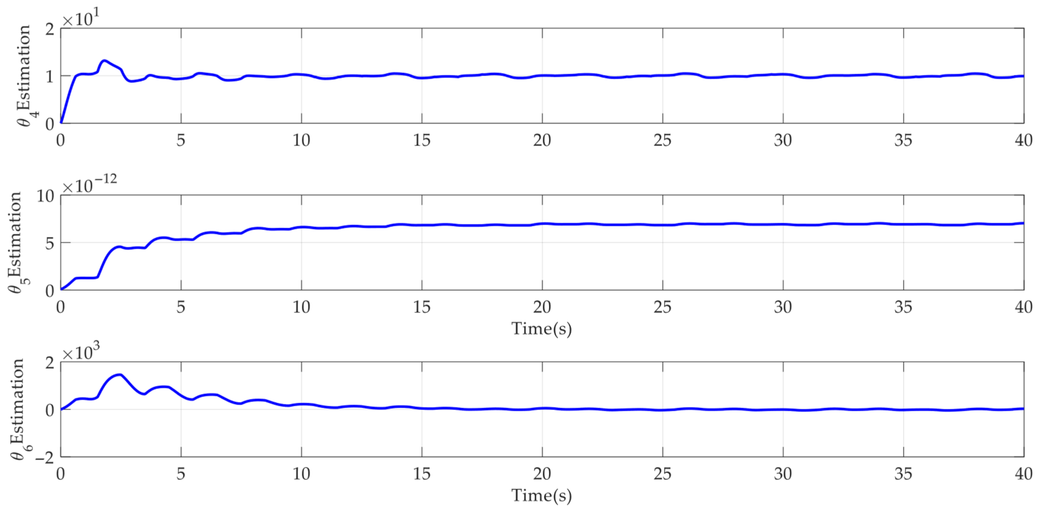
Case 2: To further verify the dynamic tracking performance of the designed AAPPC, a sine-like reference command was run. The corresponding simulation results are shown in Figure 10, Figure 11, Figure 12, Figure 13, Figure 14, Figure 15 and Figure 16. It can be seen from Figure 10 that AAPPC still delivers excellent asymptotic tracking performance, with a steady-state tracking error of approximately 2 × 10⁻³ mm. The tracking error curves of AAPPC and AAC are shown in Figure 11, in which it can be seen that the tracking error z1 of AAPPC is still always within the set safety performance boundary and surpasses that of AAC, verifying the performance consistency of the controller proposed in this paper. In addition, it can be seen in Figure 12 and Figure 13 that the estimates of the unknown time-varying parameters and disturbances of the system both still have good convergence performance, thereby verifying the effectiveness of the designed parameter adaptive law in AAPPC. The control errors z2 and z3 of AAPPC are shown in Figure 14 and Figure 15, respectively, in which z2 and z3 can be seen to be still within the set safety performance boundary range. In Figure 16, it can be seen that the control input curve in AAPPC is smooth and continuous. Consequently, Case 2 also verifies the merits of the presented control method.
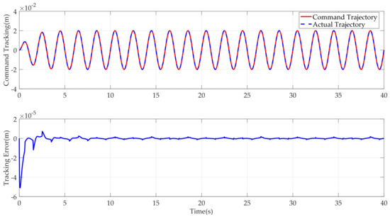
Figure 10.
Tracking performance of AAPPC.
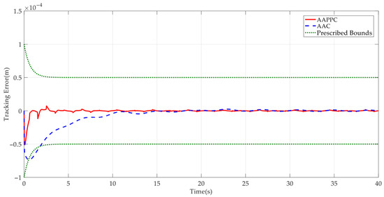
Figure 11.
Tracking errors of compared controllers.
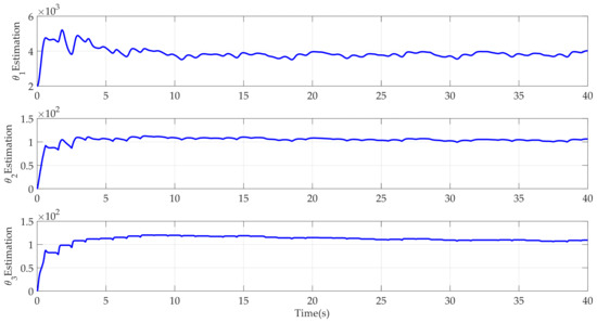
Figure 12.
Estimation of θ1~θ3 in AAPPC.
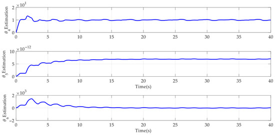
Figure 13.
Estimation of θ4~θ6 in AAPPC.
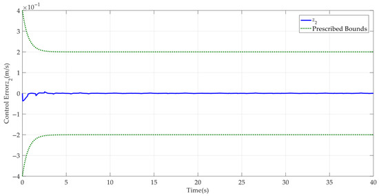
Figure 14.
Control error z2 in AAPPC.
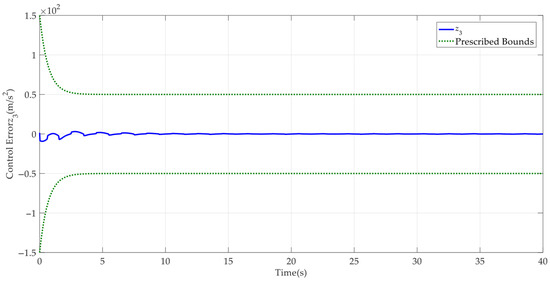
Figure 15.
Control error z3 in AAPPC.
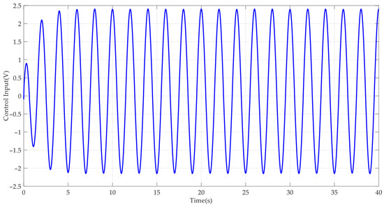
Figure 16.
Control input in AAPPC.
5. Conclusions
In this paper, we present an adaptive full-state prescribed performance position tracking controller for hydraulic systems, in which both the transient and steady performance of all the control errors can be prescribed. First, a smooth nonlinear term was skillfully introduced into the controller design so that it could simultaneously cope with both unknown time-varying parameters and disturbances. Next, by co-designing the Lyapunov Function, we enabled both the prescribed transient performance and the asymptotic steady performance of all the control errors to be achieved with the exploited controller. Finally, the merits of the proposed controller were also validated by comparative simulation results. Compared to an existing adaptive controller without full-state prescribed performance functions, the steady tracking accuracy of the hydraulic system was found to increase by 50%.
However, the adaptive full-state prescribed performance position tracking controller for hydraulic systems developed in the present study relies on the initial values of all the control errors. This may lead to restrictions in application owing to the unknown initial state values. In the future, the possibility of an initial-restriction-free full-state prescribed performance position tracking controller for hydraulic systems may be worth studying.
Author Contributions
Formal analysis, J.S. and X.Y.; investigation, J.S., J.W. and J.G.; methodology, J.S. and X.Y.; project administration, X.Y.; writing—original draft, J.S. and X.Y. All authors have read and agreed to the published version of the manuscript.
Funding
This research was not supported by any funding.
Data Availability Statement
No new data were created or analyzed in this study. Data sharing is not applicable to this article.
Conflicts of Interest
Authors Junqiang Shi and Jingcheng Gao were employed by the company Beijing Research Institute of Automation for Machinery Industry Co., Ltd. Author Jinjun Wu was employed by the company Machinery Technology Development Co., Ltd. The remaining authors declare that the research was conducted in the absence of any commercial or financial relationships that could be construed as a potential conflict of interest.
References
- Yao, J.; Jiao, Z.; Ma, D.; Yan, L. High-accuracy tracking control of hydraulic rotary actuators with modeling uncertainties. IEEE/ASME Trans. Mechatron. 2014, 19, 633–641. [Google Scholar] [CrossRef]
- Yao, J.; Deng, W. Active Disturbance Rejection Adaptive Control of Hydraulic Servo Systems. IEEE Trans. Ind. Electron. 2017, 64, 8023–8032. [Google Scholar] [CrossRef]
- Sun, W.; Pan, H.; Gao, H. Filter-Based Adaptive Vibration Control for Active Vehicle Suspensions with Electrohydraulic Actuators. IEEE Trans. Veh. Technol. 2016, 65, 4619–4626. [Google Scholar] [CrossRef]
- Won, D.; Kim, W.; Tomizuka, M. High-gain-observer-based integral sliding mode control for position tracking of electrohydraulic servo systems. IEEE/ASME Trans. Mechatron. 2017, 22, 2695–2704. [Google Scholar] [CrossRef]
- Pan, H.; Sun, W. Nonlinear Output Feedback Finite-Time Control for Vehicle Active Suspension Systems. IEEE Trans. Ind. Inform. 2019, 15, 2073–2082. [Google Scholar] [CrossRef]
- Huang, Y.; Pool, D.M.; Stroosma, O.; Chu, Q. Long-stroke hydraulic robot motion control with incremental nonlinear dynamic inversion. IEEE/ASME Trans. Mechatron. 2019, 24, 304–314. [Google Scholar] [CrossRef]
- Zhang, J.; Liu, S.; Huang, W.; Lyu, F.; Xu, H.; Yan, R.; Xu, B. A Cylinder Block Dynamic Characteristics-Based Data Augmentation Method for Wear State Identification under Data Imbalance Condition. Mech. Syst. Signal Process. 2024, 208, 111036. [Google Scholar] [CrossRef]
- Jiao, Z.; Chen, X.; Liu, X.; Li, X.; Qi, P.; Shang, Y.; Qiao, W. An Experimental Study on Outer Frame Position Control of Hydraulic Flight Motion Simulator With Model Compensation. IEEE/ASME Trans. Mechatron. 2022, 27, 3419–3428. [Google Scholar] [CrossRef]
- Chen, Z.; Zhou, S.; Shen, C.; Lyu, L.; Zhang, J.; Yao, B. Observer-Based Adaptive Robust Precision Motion Control of a Multi-Joint Hydraulic Manipulator. IEEE/CAA J. Autom. Sin. 2024, 11, 1213–1226. [Google Scholar] [CrossRef]
- Yang, X.; Ge, Y.; Deng, W.; Yao, J. Precision Motion Control for Electro-Hydraulic Axis Systems under Unknown Time-Variant Parameters and Disturbances. Chin. J. Aeronaut. 2024, 37, 463–471. [Google Scholar] [CrossRef]
- Guo, Q.; Zhang, Y.; Celler, B.G.; Su, S.W. Backstepping Control of Electro-Hydraulic System Based on Extended-State-Observer with Plant Dynamics Largely Unknown. IEEE Trans. Ind. Electron. 2016, 63, 6909–6920. [Google Scholar] [CrossRef]
- Na, J.; Li, Y.; Huang, Y.; Gao, G.; Chen, Q. Output Feedback Control of Uncertain Hydraulic Servo Systems. IEEE Trans. Ind. Electron. 2020, 67, 490–500. [Google Scholar] [CrossRef]
- Ba, D.X.; Dinh, T.Q.; Bae, J.; Ahn, K.K. An Effective Disturbance-Observer-Based Nonlinear Controller for a Pump-Controlled Hydraulic System. IEEE/ASME Trans. Mechatron. 2020, 25, 32–43. [Google Scholar] [CrossRef]
- Yao, B.; Al-Majed, M.; Tomizuka, M. High-Performance Robust Motion Control of Machine Tools: An Adaptive Robust Control Approach and Comparative Experiments. IEEE/ASME Trans. Mechatron. 1997, 2, 63–76. [Google Scholar]
- Mohanty, A.; Yao, B. Integrated Direct/Indirect Adaptive Robust Control of Hydraulic Manipulators with Valve Deadband. IEEE/ASME Trans. Mechatron. 2011, 16, 707–715. [Google Scholar] [CrossRef]
- Helian, B.; Chen, Z.; Yao, B.; Lyu, L.; Li, C. Accurate Motion Control of a Direct-Drive Hydraulic System with an Adaptive Nonlinear Pump Flow Compensation. IEEE/ASME Trans. Mechatron. 2021, 26, 2593–2603. [Google Scholar] [CrossRef]
- Helian, B.; Chen, Z.; Yao, B. Constrained Motion Control of an Electro- Hydraulic Actuator Under Multiple Time-Varying Constraints. IEEE Trans. Ind. Inform. 2023, 19, 11878–11888. [Google Scholar] [CrossRef]
- Lyu, L.; Chen, Z.; Yao, B. Advanced Valves and Pump Coordinated Hydraulic Control Design to Simultaneously Achieve High Accuracy and High Efficiency. IEEE Trans. Control Syst. Technol. 2021, 29, 236–248. [Google Scholar] [CrossRef]
- Yao, J.; Deng, W.; Sun, W. Precision Motion Control for Electro-Hydraulic Servo Systems with Noise Alleviation: A Desired Compensation Adaptive Approach. IEEE/ASME Trans. Mechatron. 2017, 22, 1859–1868. [Google Scholar] [CrossRef]
- Wang, C.; Quan, L.; Jiao, Z.; Zhang, S. Nonlinear Adaptive Control of Hydraulic System with Observing and Compensating Mismatching Uncertainties. IEEE Trans. Control Syst. Technol. 2018, 26, 927–938. [Google Scholar] [CrossRef]
- Deng, W.; Yao, J. Extended-State-Observer-Based Adaptive Control of Electrohydraulic Servomechanisms without Velocity Measurement. IEEE/ASME Trans. Mechatron. 2020, 25, 1151–1161. [Google Scholar] [CrossRef]
- Yang, X.; Yao, J.; Deng, W. Output feedback adaptive super-twisting sliding mode control of hydraulic systems with disturbance compensation. ISA Trans. 2021, 109, 175–185. [Google Scholar] [CrossRef] [PubMed]
- Ilchmann, A.; Ryan, E.P.; Townsend, P. Tracking Control with Prescribed Transient Behaviour for Systems of Known Relative Degree. Syst. Control Lett. 2006, 55, 396–406. [Google Scholar] [CrossRef]
- Yang, X.; Deng, W.; Yao, J. Neural Adaptive Dynamic Surface Asymptotic Tracking Control of Hydraulic Manipulators With Guaranteed Transient Performance. IEEE Trans. Neural Netw. Learn. Syst. 2023, 34, 7339–7349. [Google Scholar] [CrossRef]
- Yang, X.; Ge, Y.; Zhu, W.; Deng, W.; Zhao, X.; Yao, J. Adaptive Motion Control for Electro-Hydraulic Servo Systems With Appointed-Time Performance. IEEE/ASME Trans. Mechatron. 2025; early access. [Google Scholar] [CrossRef]
- Xu, Z.; Deng, W.; Shen, H.; Yao, J. Extended-State-Observer-Based Adaptive Prescribed Performance Control for Hydraulic Systems With Full-State Constraints. IEEE/ASME Trans. Mechatron. 2022, 27, 5615–5625. [Google Scholar] [CrossRef]
- Xu, Z.; Sun, C.; Hu, X.; Liu, Q.; Yao, J. Barrier Lyapunov Function-Based Adaptive Output Feedback Prescribed Performance Controller for Hydraulic Systems With Uncertainties Compensation. IEEE Trans. Ind. Electron. 2023, 70, 12500–12510. [Google Scholar] [CrossRef]
- Guo, Q.; Zhang, Y.; Celler, B.G.; Su, S.W. Neural Adaptive Backstepping Control of a Robotic Manipulator with Prescribed Performance Constraint. IEEE Trans. Neural Netw. Learn. Syst. 2019, 30, 3572–3583. [Google Scholar] [CrossRef]
- Merritt, H. Hydraulic Control Systems; John Wiley & Sons: Hoboken, NJ, USA, 1967. [Google Scholar]
- Krstic, M.; Kanellakopoulos, I.; Kokotovic, P. Nonlinear and Adaptive Control Design; Wiley: New York, NY, USA, 1995. [Google Scholar]


Disclaimer/Publisher’s Note: The statements, opinions and data contained in all publications are solely those of the individual author(s) and contributor(s) and not of MDPI and/or the editor(s). MDPI and/or the editor(s) disclaim responsibility for any injury to people or property resulting from any ideas, methods, instructions or products referred to in the content. |
© 2025 by the authors. Licensee MDPI, Basel, Switzerland. This article is an open access article distributed under the terms and conditions of the Creative Commons Attribution (CC BY) license (https://creativecommons.org/licenses/by/4.0/).