Abstract
In the realm of 3D curve reconstruction, Non-Uniform Rational B-Splines (NURBSs) offer a versatile mathematical tool due to their ability to precisely represent complex geometries. However, achieving high fitting accuracy in stereo-based applications remains challenging, primarily due to the nonlinear nature of weight optimization. This study introduces an enhanced iterative strategy that leverages the geometric significance of NURBS weights to incrementally refine curve fitting. By formulating an inverse optimization problem guided by model deformation principles, the proposed method progressively adjusts weights to minimize reprojection error. Experimental evaluations confirm the method’s convergence and demonstrate its superiority in fitting accuracy when compared to conventional optimization techniques.
Keywords:
two-view geometry; iterative optimization; curve fitting; geometric optimization; reprojection error minimization; NURBS MSC:
68T45
1. Introduction
Stereo reconstruction has gained significant importance across various practical domains due to its ability to enable automatic and real-time analysis. Fields such as autonomous navigation, augmented reality, surveillance, object tracking, and military applications rely heavily on robust reconstruction techniques due to their reliability, flexibility, and adaptability. Most existing approaches to 3D reconstruction adopt a model-driven framework, where the geometry of objects is approximated using basic primitives such as cubes, spheres, cylinders, and other parametric forms. Although these techniques are easy to use and simple, more basic shapes or scene decompositions are required when dealing with complicated or free-form structures. In numerous fields, non-uniform rational B-spline (NURBS) curves have been utilized extensively because of their exceptional mathematical characteristics and modeling versatility.
Enhancing the fitting accuracy in NURBS-based engineering applications remains a critical challenge. To address this, extensive research has been carried out on the optimization of control points, the refinement of knot vectors, the adjustment of datapoint parameters, and the modification of weights. Although least-squares fitting is commonly used to compute control points [1], it becomes inefficient for large datasets and lacks flexibility for local refinements due to its inability to use intermediate updates. To overcome these limitations, progressive iterative approximation algorithms and their advanced variants have been proposed [2,3], offering better local control and scalability, albeit with a trade-off in computational efficiency compared to direct least-squares fitting. Optimization of data parameters and weights has been relatively less explored. Ma introduced a projection technique for the base curve to refine the data parameters, although the underlying optimization strategy was not fully elaborated [4]. For weight adjustment, symmetric eigenvalue decomposition has been used to estimate weight values [5]; however, the lack of a clear geometric interpretation restricts its practical applicability. Furthermore, Zhang proposed using simulated annealing for weight optimization [6], a method that, while flexible, is highly dependent on expert-defined search boundaries and suffers from slow convergence. More recently, Meng suggested using the least-squares progressive iterative approximation (LSPIA) method for weight adjustment [7], although it still faces challenges in achieving high optimization efficiency.
The task of identifying the optimal number and distribution of knots for the approximation of the B-spline curve while adhering to a specified error threshold is known as knot optimization. This remains a complex challenge for two main reasons. First, the unknown quantity and locations of knots introduce substantial nonlinearity and computational difficulty into the problem. Second, it is inherently challenging to derive analytical expressions or general principles governing optimal knot placement, especially when dealing with arbitrary or noisy datasets. Early approaches aimed at addressing this problem focused on achieving a more uniform knot distribution in the parameter domain by averaging geometric features of the data points, thereby stabilizing the system of equations used for the fitting of the B-spline [1]. Subsequently, a binary search-based method was introduced to determine the maximum allowable span between knots while satisfying an approximation error constraint, significantly improving computational performance but occasionally resulting in discontinuities in the approximation [8]. Another significant development framed the knot placement task as a convex optimization problem, where both the number and location of knots are optimized simultaneously to minimize the overall approximation error. This strategy provides high accuracy but incurs a greater computational cost due to its iterative nature [9]. More recently, data-driven techniques such as machine learning have been utilized for this purpose. For example, Laube et al. [10] employed support vector machines to learn effective knot placement patterns from training data, offering an adaptive and automated solution to knot distribution. The applicability of their method to datasets other than the training dataset is limited by its heavy dependence on the training dataset. There is also a corpus of research on knot vector optimization that makes use of genetic algorithms [11,12]. Usually computationally costly, these approaches yield globally suboptimal results. A different corpus of research suggests heuristic techniques [13,14,15] that direct knot placement utilizing particular attributes of the incoming dataset. Specifically, curvature is a frequently employed criterion in heuristic approaches. These heuristic approaches also employ derivatives for knot placement. In conventional reconstruction methods, derivatives of input data are typically approximated by employing piecewise low-degree polynomial functions. Breakpoints—or joining points between adjacent polynomial segments—are then utilized as candidate knot locations to construct a more flexible and accurate representation of B-spline data [1]. While this approach facilitates a localized approximation and provides computational simplicity, it often struggles to ensure global smoothness and optimal distribution of knots, particularly for complex or noisy datasets. Hence, an effective strategy must balance computational efficiency with fitting precision.
We aimed to improve the reconstruction accuracy of space curves obtained from two views while also reducing reliance on manual correspondence across image planes. Our main contributions can be summarized as follows: (1) We use a novel iterative optimization strategy inspired by the principles of the active contour (snake) model specifically adapted for the reconstruction of 3D NURBS curves. The method dynamically adjusts control-point weights and refines datapoint parameterizations to improve curve accuracy. (2) Additionally, we adopt a systematic method for automatic insertion of knots and control points. Unlike traditional methods where knot locations are predefined or manually selected, this technique adaptively identifies regions requiring higher flexibility and dynamically introduces new knots and control points based on fitting error metrics. This automated mechanism allows the model to better capture intricate geometrical features of the underlying 3D structure without excessive human intervention.
Through these adaptations, the proposed framework ensures that the reconstructed curve adheres closely to the stereo projections while maintaining smoothness, flexibility, and robustness, even under imperfect data conditions. The remainder of this paper is organized as follows: Section 2 details the parameter and weight-based reconstruction methodology. Section 3 presents implementation steps and experimental results. Section 4 discusses statistical validation, and Section 5 concludes with a summary of key findings and future directions.
2. Parameter- and Weight-Based Reconstruction
This section describes our optimization-driven method for reconstructing space curves by systematically adjusting various parameters, including knot-vector insertion, parameter re-estimation, and weight-vector refinement. The focus is placed entirely on the reconstruction stage under the assumption that the 2D image data points and the projection matrices have already been extracted through existing techniques [16]. To reconstruct free-form 3D curves, the NURBS model is commonly employed due to its flexibility and precision in handling complex geometries. Employing NURBSs enables the transformation of the 3D reconstruction problem into the recovery of appropriate control points and associated weights, effectively modeling the curve’s geometric structure.
The NURBS framework provides a unified mathematical approach capable of accurately representing both fundamental algebraic shapes and highly flexible free-form curves. Due to its rational formulation, it offers precise control over curve behavior and excellent flexibility in handling complex geometries. Furthermore, the NURBS structure inherently guarantees smoothness and continuity across the curve, satisfying both geometric and parametric constraints without manual tuning. Another important property is that a NURBS curve maintains its essential characteristics under perspective, affine, and rigid body transformations, making it highly robust for real-world applications. These unique attributes underline the extensive adoption of NURBS within domains such as Computer-Aided Geometric Design (CAGD) and related fields [17].
A NURBS curve of order k in a 3D space is mathematically described by
In the above notation, represents the control point, and denotes the rational B-spline basis function, which is described as follows:
where denotes the weight associated with the control point (). represents the B-spline basis function of order k evaluated for the parameter, which is computed using the de Boor recursion formula:
where represents the individual knots that collectively form the knot vector (). Typically, the knot vector is normalized within the interval . A clamped knot vector is used, meaning that the first k and last k knots are repeated, ensuring that the curve precisely interpolates the first and last control points. The internal knots are determined using the normalized knot parameterization technique (NKPT) [18], and the entire knot vector must be in non-decreasing order, which provides a stable system for the computation of control points.
The construction of the knot vector closely follows the definition of datapoint parameters to avoid singularities in the resulting system of equations during the extraction of the control point. Parameter values are initially set within the range of , ensuring a uniform distribution across the domain. Additional parameter values are calculated based on the cumulative chord-length strategy, which distributes the parameters proportionally to the spatial distances between successive data points, such as
where is the parameter corresponding to the data point.
In this study, we explore the process of reconstructing 3D space curves from stereo images by leveraging the perspective-invariant properties of NURBS models. Assume that the set of j chaotic data points in the stereo image planes generated by the 2D reconstruction techniques is designated by . The 3D NURBS curve () must be created so that the collection of data points () can be accurately approximated by its projection () in the image planes. To solve this non-linear optimization problem, we adopt an energy minimization-based methodology as follows:
To begin, we introduce the energy function () that characterizes the objective of our optimization framework:
In this formulation, the internal energy component () regulates the smoothness of the curve. To estimate the differential characteristics of NURBS curves, associated derivatives are employed and can be expressed as follows:
where , , and are non-negative constants that must be predefined prior to initiating the optimization procedure [19].
To formulate the external energy (), a distance minimization strategy is applied to quantify the proximity of the evolving projected curve to the corresponding 2D data points (), expressed as
where represents the point on the projected NURBS curve corresponding to the parameter and denotes the coordinates of the planar data point in the image plane.
A nonlinear optimization strategy is applied to fit a NURBS curve to data obtained by projecting a free-form 3D curve onto two perspective image planes. This fitting technique, known as the NURBS snake-based method, seeks to minimize the cost function defined in Equation (6), as outlined by Saini et al. [20]. In this approach, both the positions of the control points and their associated weights are optimized simultaneously, treating them as variables within the solution space. To enhance convergence and maintain robustness during the optimization process, the Levenberg–Marquardt algorithm is employed, preceded by a two-phase initialization procedure designed to stabilize the iterative fitting process [16].
At the outset, although the optimization successfully reduces the error between the sample points and their corresponding projections on the NURBS curve, several parameters—such as the knot vector, parameter values assigned to the data points, and initial weight estimates—are kept constant. Therefore, it is necessary to extend the optimization to include these parameters. The following methodology adopts strategies to incorporate these elements into the optimization process.
- Parameter Optimization: Traditional parameterization techniques often lack sufficient precision, resulting in inaccurate estimation of the data point parameters on the final fitted curve. To enhance the fitting accuracy, it becomes essential to update the data point parameters. This requires identifying the nearest points on the NURBS curve [21], which serve to refine the parameter values and improve the curve fitting. The closest locations on the NURBS curve are determined using an iterative approach, as described below:where represents the nearest point on the fitting curve. In this process, the initial value for the iteration is chosen as the parameter obtained from the preceding two-step fitting procedure [20]. This approach ensures accurate determination of the nearest point while also enhancing computational efficiency.
- Weight Optimization: In a NURBS curve, the weights assigned to control points influence the curve’s shape in a geometrically intuitive way: increasing a weight draws the curve closer to that control point, while reducing the weight causes the curve to move away from it. By leveraging this geometric property, the fitting curve can be further refined to achieve higher accuracy. The objective function [21] used for optimizing the weights is defined as follows:where d represents the distance between the planar data point and the estimated point on the fitting NURBS curve, shows the change in weight, and shows the extent and direction of influence of weight given byThe set of equations can be organized into a matrix form as follows.Singular Value Decomposition (SVD) [21,22] provides the solution to the aforementioned system. The weight adjustments that reduce error comprise this group of solutions. Weight optimization is accomplished by introducing incremental changes to the existing curve’s weights. The fitting accuracy improves progressively through repeated updates to the weights, combined with parameter refinement in each iteration.
The procedure for fitting a NURBS curve through simultaneous optimization of parameters and weights is organized as follows:
- Step 1: Specify a suitable initial configuration for the 3D NURBS curve.
- Step 2: Project the 3D curve onto both image planes using the calibrated projection matrices.
- Step 3: Determine how many knots are needed and construct the knot vector based on a normalized parameterization approach [18].
- Step 4: Generate the initial NURBS approximation through the two-stage fitting protocol [20]. Compute the external energy (Equation (8)) across all planar data points, followed by joint optimization of data parameters and control-point weights.
- Step 5: Evaluate whether the current fitting error satisfies predefined thresholds. If acceptable, finalize the process. Otherwise, insert additional knots forparameters exhibiting maximum residual error and refine datapoint assignments via nearest-point iteration (Equation (9)).
- Step 6: Recompute control points using the updated knot sequence, optimized parameters, and adjusted weights as per the triangulation framework [20].
- Step 7: Reconstruct spatial control points and weights using multi-view geometric constraints [1]; then, regenerate the 3D curve. Calculate internal energy using Equation (7).
- Step 8: Optimize the 3D control points iteratively to minimize the combined energy functional (Equation (6)), ensuring tighter alignment of projections with 2D data.
- Step 9: Repeat Steps 2–8 until convergence to the target accuracy. The refined NURBS curve constitutes the final reconstruction.
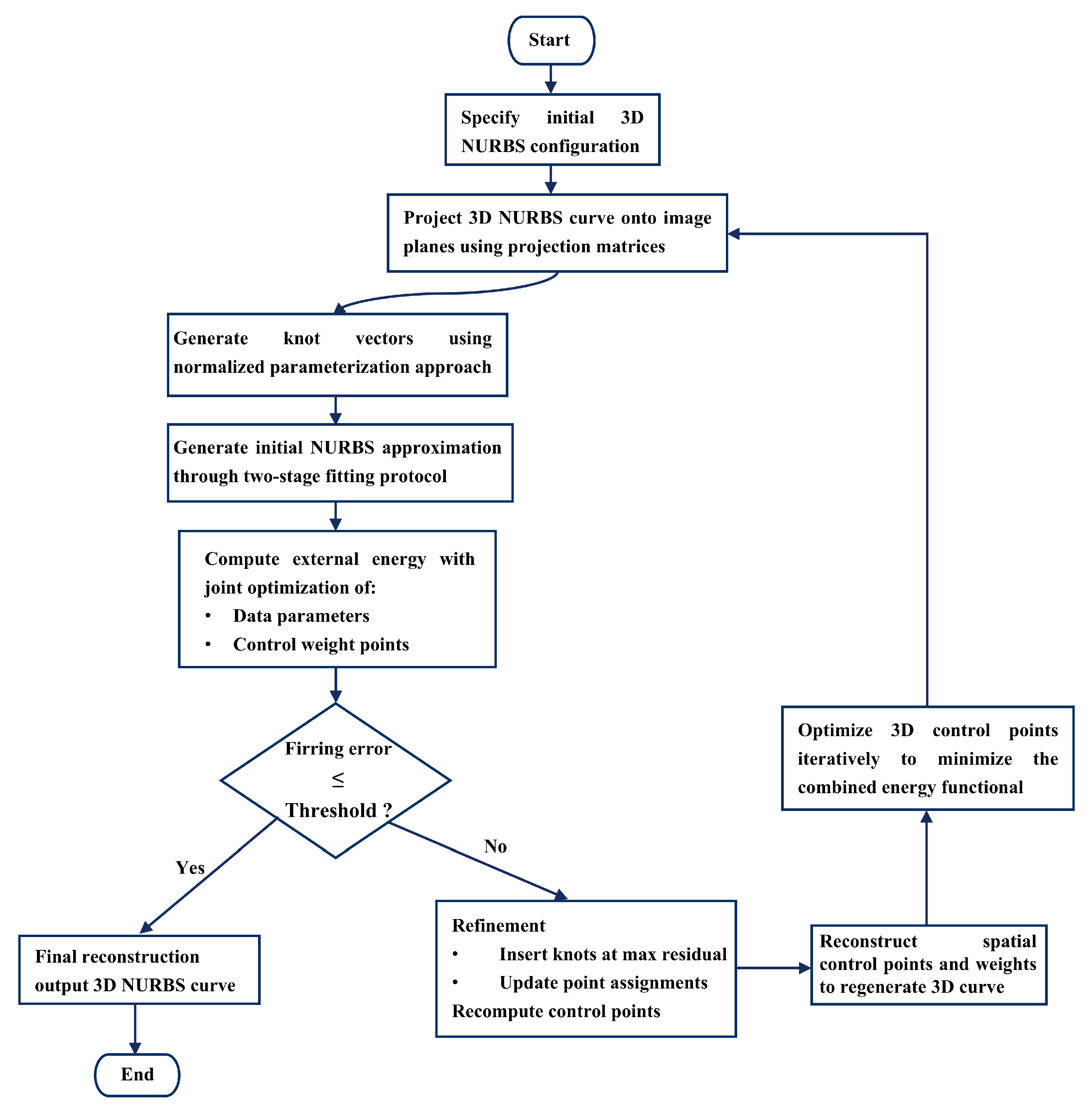
The proposed optimization-driven NURBS reconstruction method effectively addresses several practical challenges encountered in real-world stereo reconstruction scenarios. By jointly optimizing data parameters and control-point weights using external energy minimization (Figure 1), the method dynamically adapts to local geometrical characteristics, thereby improving resilience against noise and sampling irregularities. Furthermore, the use of iterative parameter refinement (Equation (9)) ensures accurate alignment, even under imperfect correspondences, while the adaptive knot insertion mechanism facilitates the reconstruction of intricate shapes without manual tuning. These capabilities, combined with global optimization based on the Levenberg-Marquardt algorithm, enable the framework to consistently achieve high accuracy and robustness in diverse application domains, such as reverse engineering, medical imaging, and robotic vision.
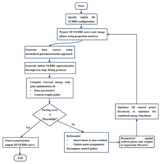
Figure 1.
Flowchart of the reconstruction process.
Figure 1 illustrates the overall workflow of the proposed optimization-driven 3D curve reconstruction framework. The process begins with initialization and projection, followed by iterative optimization of control-point weights and data parameters based on energy minimization. Adaptive knot insertion and refinement steps ensure convergence toward an accurate and smooth NURBS representation of the space curve. Algorithm 1 formalizes this iterative reconstruction workflow.
| Algorithm 1 Iterative NURBS Curve Reconstruction |
| Input: Stereo image plane data points |
| Parameterize data points on both image planes via base curve projection [16] |
| Initialize a 3D NURBS curve using a two-step fitting protocol [20]. |
| Configure knot vector U and B-spline basis order k using NKTP [1] |
| for each data point do |
| Compute external energy (Equation (8)) between projected curve and |
| end for |
| while do |
| Insert knot at (parameter with maximum ) |
| for each data point do |
| Update parameter via nearest-point iteration (Equation (9)) |
| end for |
| Optimize weights using SVD-based linear system (Equation (13)) |
| Rebuild the NURBS curve with updated , U, and [20] |
| Triangulate 3D control points from projections [16] |
| Calculate internal energy (Equation (7)) for smoothness |
| Minimize total energy (Equation (6)) via Levenberg-Marquardt |
| for each data point do |
| Re-evaluate for updated projections |
| end for |
| end while |
| Output: Refined 3D NURBS curve |
3. Implementation and Results
Let denote the projection of the NURBS curve () onto the image plane. To evaluate and compare the performance between the original and reconstructed curves, several error metrics were utilized, including the mean error (MeanErr), the maximum error (MaxErr), and the root mean square error (RmsErr), as summarized in Table 1.

Table 1.
Error metrics.
The quadratic NURBS curve must be utilized at the very least because of the first derivatives’ continuity requirement. Due to optimization of the data parameters, the second derivatives must also be continuous. At minimum, the NURBS curve must be cubic. As the order of the NURBS curve increases, the effect decreases. One of the key benefits of employing a NURBS representation lies in its ability to model complex curves accurately. This characteristic enhances the applicability of our algorithm compared to conventional curve reconstruction techniques. In challenging cases where optimizing the initial control points alone fails to capture the target data points accurately, this difficulty is addressed by automatically inserting additional control points based on adjustments to the weights and other associated parameters.
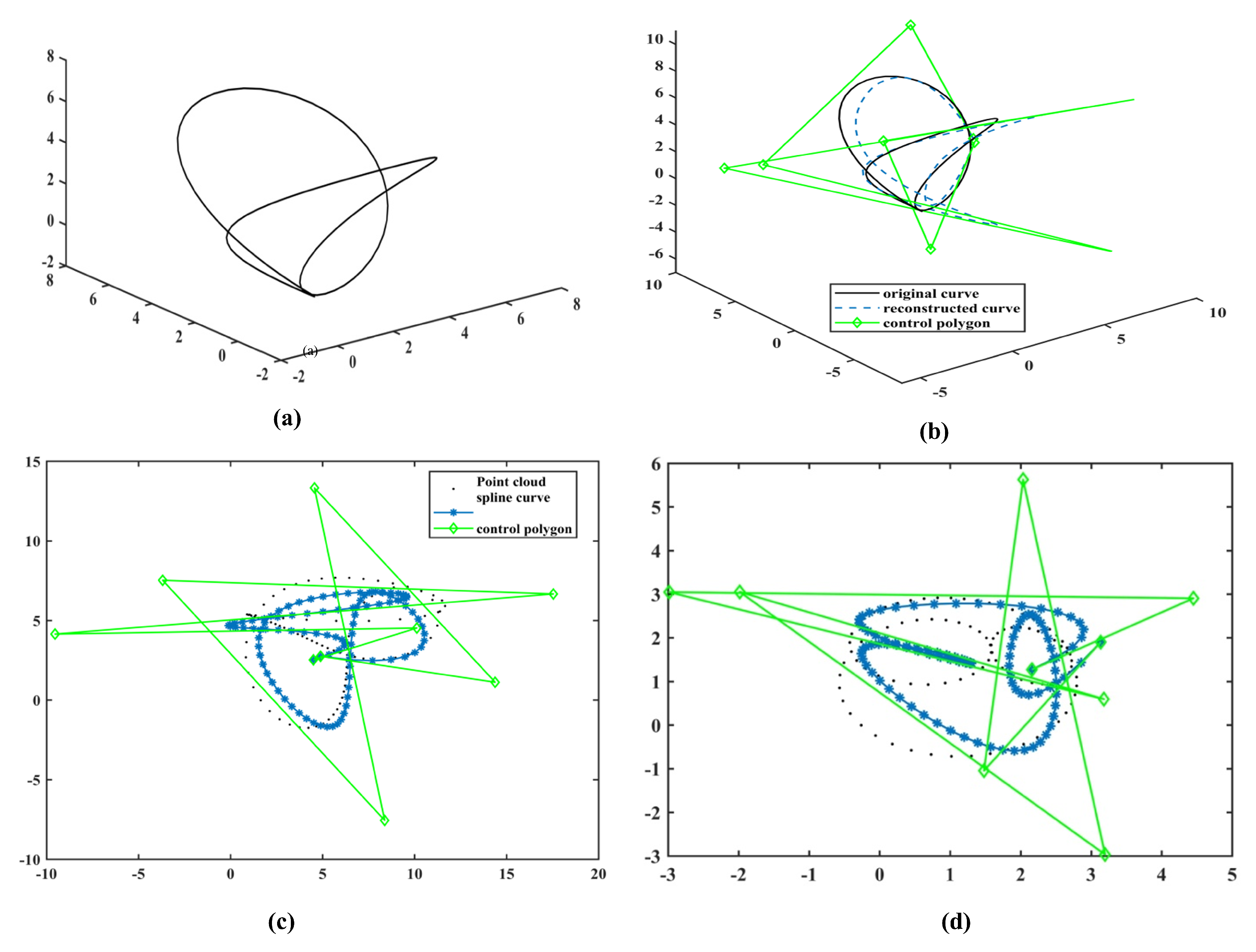
Figure 2, Figure 3 and Figure 4 illustrate the results obtained by reconstructing a closed-space curve using our proposed technique. The input for this process consists of discrete points derived from a noise-perturbed closed 3D curve, where the noise is Gaussian with zero mean and variable standard deviation (). Initially, the user manually identifies and pairs corresponding noisy point sets across the stereo image planes. These correspondences serve as the basis for initializing the NURBS control polygon using a dual-phase fitting strategy inspired by the methodology proposed in [16].
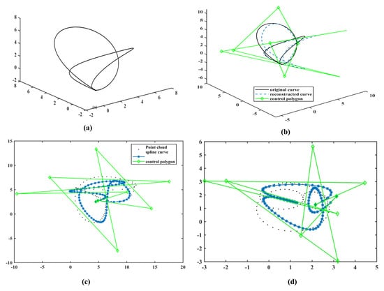
Figure 2.
Reconstruction outcomes for a closed curve are illustrated as follows: (a) the original 3D curve; (b) the reconstructed 3D curve obtained using nine evolved control points; (c,d) 2D projections of both the initial and reconstructed curves in the left and right image planes, respectively.
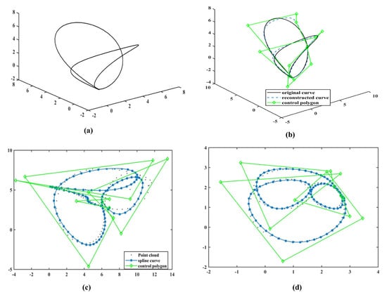
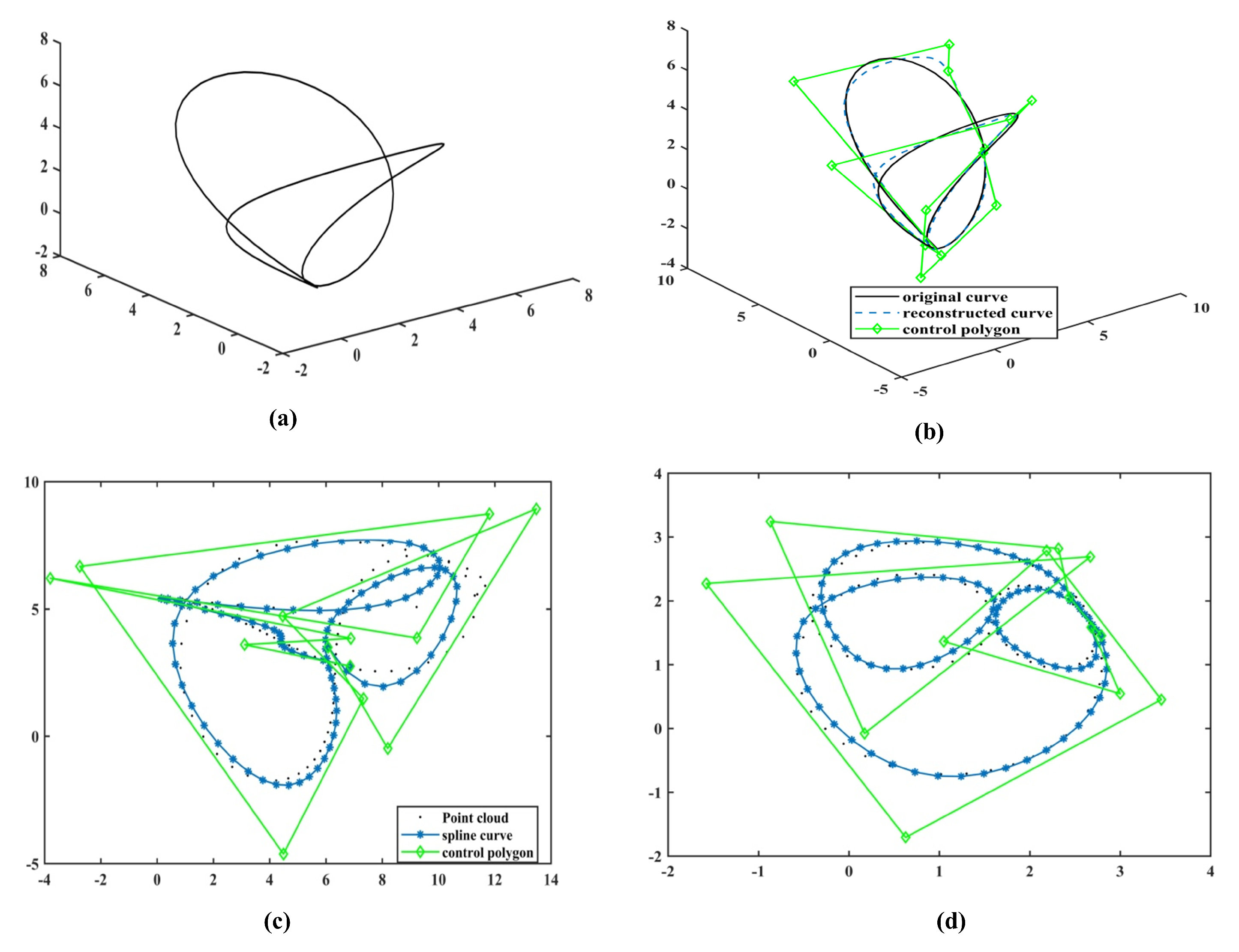
Figure 3.
The reconstruction results for a closed curve are depicted as follows: (a) the original 3D curve; (b) the reconstructed 3D curve using 13 refined control points; (c,d) the 2D projections of both the initial and reconstructed curves in the left and right image planes, respectively.
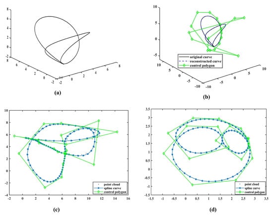
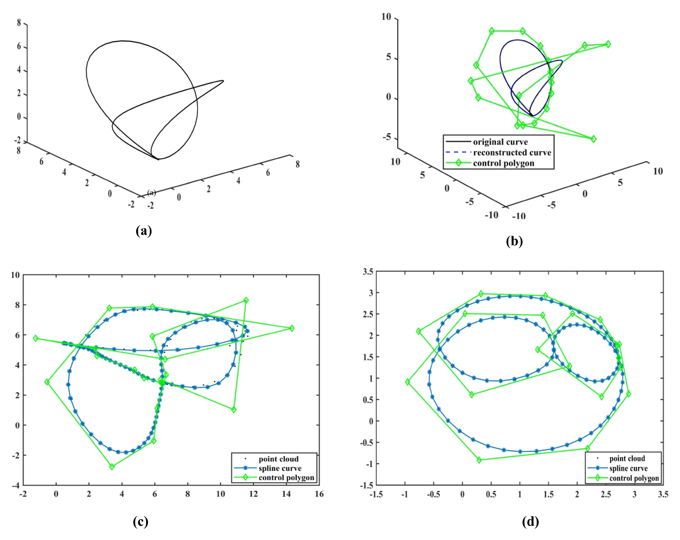
Figure 4.
The reconstruction outcomes for a closed curve are illustrated as follows: (a) the original 3D curve; (b) the reconstructed 3D curve obtained with 20 evolved control points; (c,d) the 2D projections of the initial and reconstructed curves in the left and right image planes, respectively.
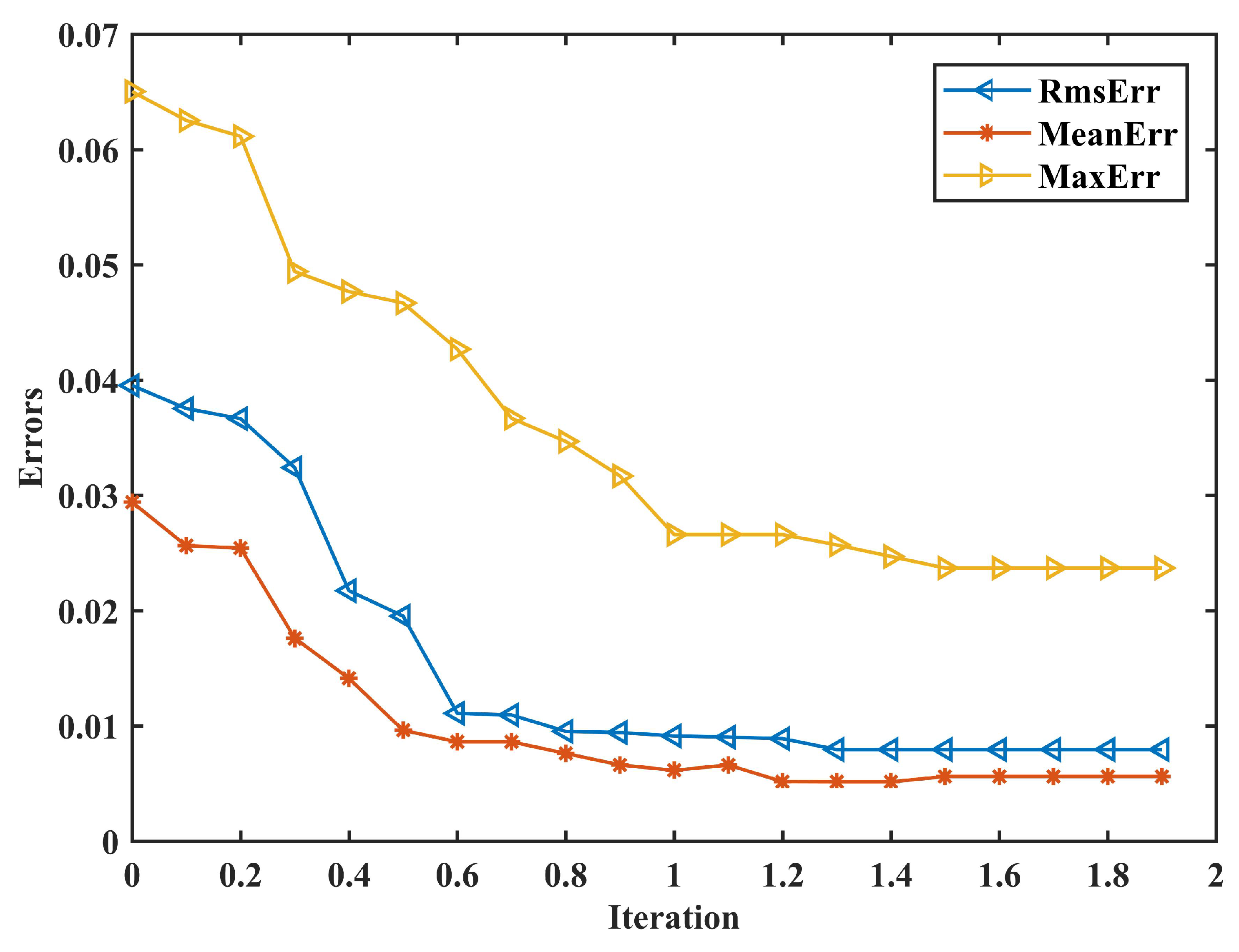
The fitting results in the two view planes are shown in Figure 2c,d. Although the locations of the control points in the reconstructed 3D result at this stage (Figure 2b) are not precise, we may observe a gradual decrease in approximation errors after further iterations, and the final result fits the data points quite accurately (Figure 4c,d). Figure 2b shows the reconstruction result with 9 control points, while Figure 3b shows the result with 13 control points. Figure 4b shows the final result with 20 control points that appear the same as the original curve. Figure 5 shows the reconstruction errors as a function of iterations.
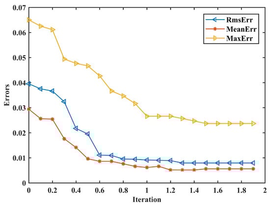
Figure 5.
Variation of reconstruction errors with respect to the number of iterations for a closed curve.
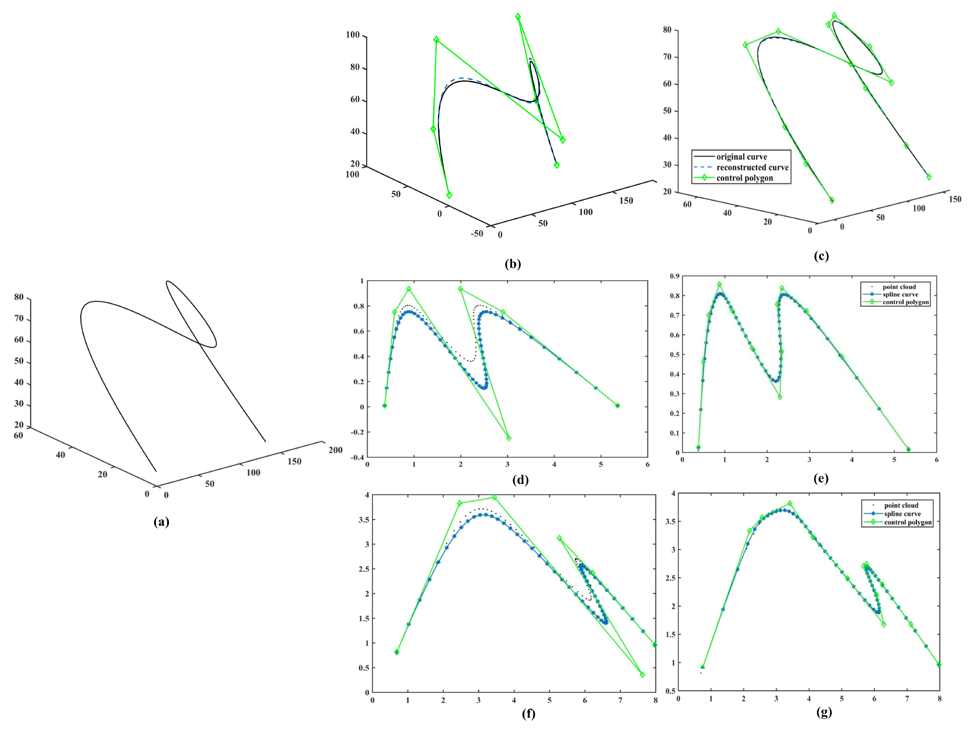
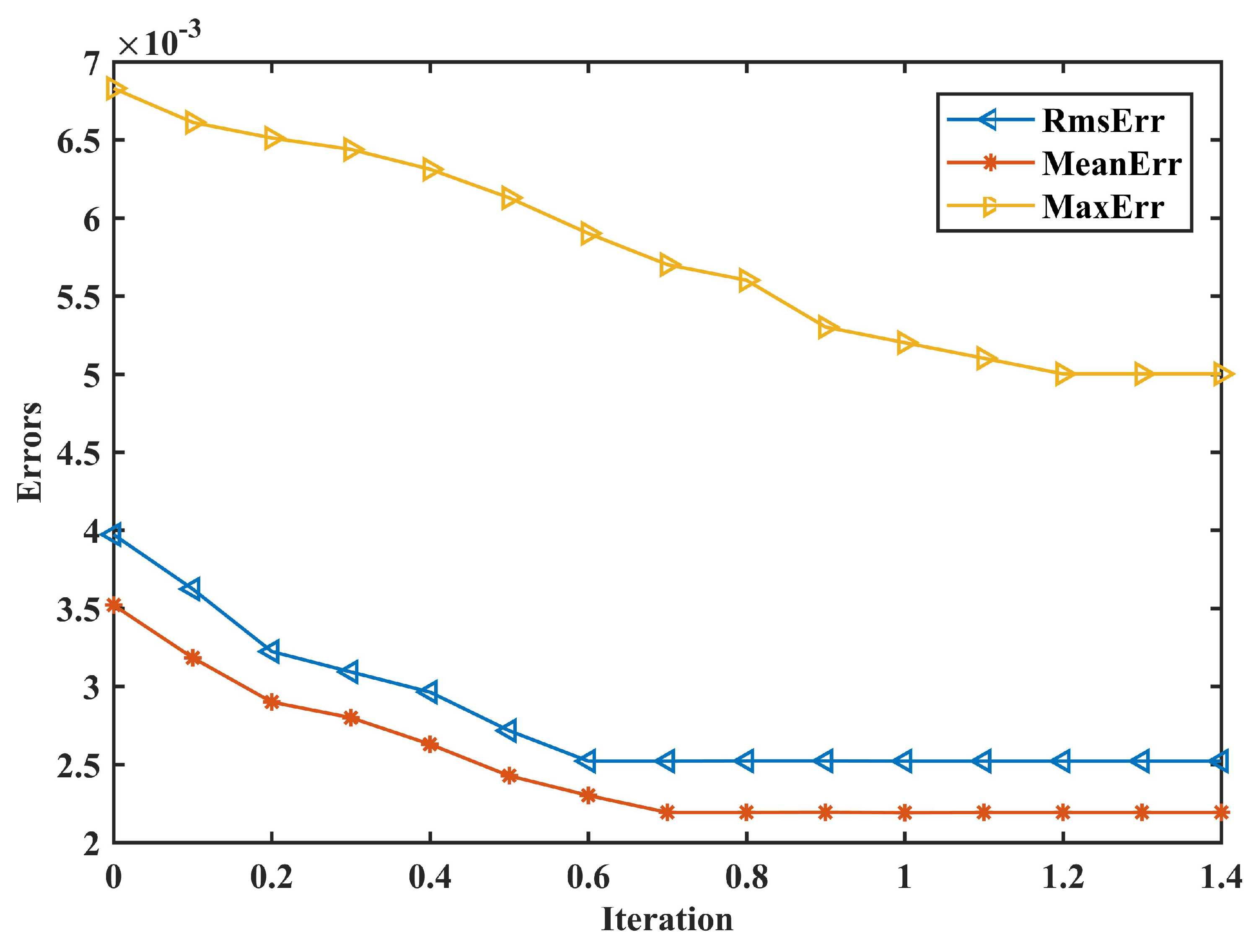
Data points obtained from an open space curve (Figure 6a) can be successfully reconstructed using our method. The same procedure is used for the reconstruction. The fitting results are shown in the left view (Figure 6d,e) and the right view (Figure 6f,g). Figure 6b,c show the reconstruction results that evolve with the 7 and 13 control points, respectively. Here, we can observe that the iteration procedure reconstructs the curve very well with 13 control points. Reconstruction errors, as a function of iterations in this case, are shown in Figure 7, which shows that the approximation errors are reduced and the curve becomes stable very quickly.
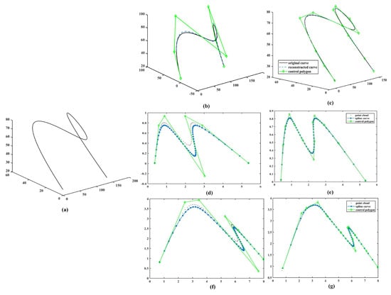
Figure 6.
Reconstruction results for an open curve are shown as follows: (a) the original 3D curve; (b,c) reconstructed 3D curves using 7 and 13 evolved control points, respectively; (d,f) 2D projections of the initial and reconstructed curves in the left and right views; (e,g) 2D projections of the initial and reconstructed curves in the left and right views, respectively.
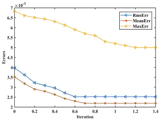
Figure 7.
Reconstruction errors versus number of iterations for an open curve.
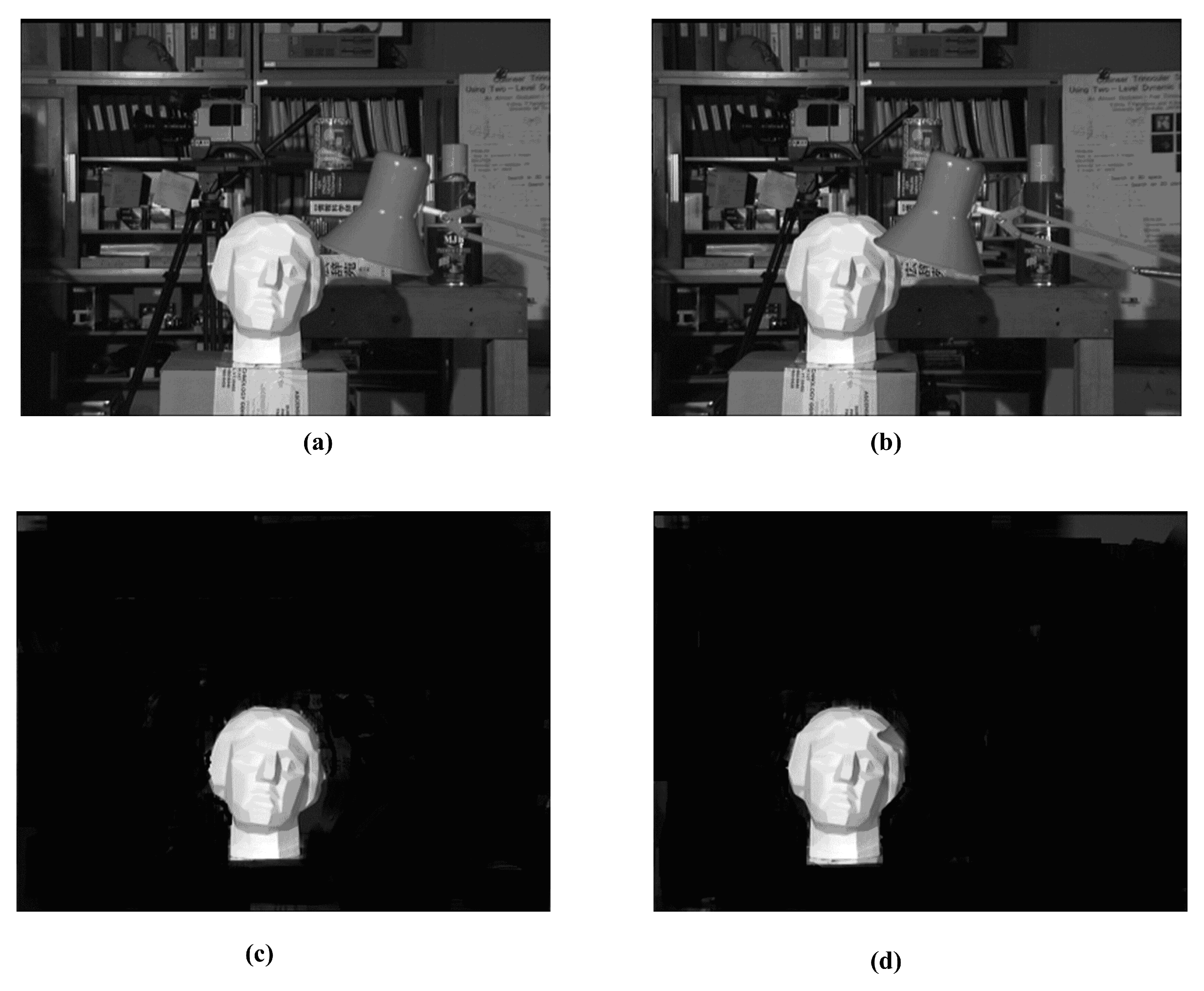
Finally, the reconstruction yields the real world of pictures. We used the Tsukuba pictures, which were made public several years ago, for this. Once more, we took the two following frames (Figure 8a,b) of the Tsukuba image taken from slightly different perspectives to perform the two-view reconstruction. Rebuilding the 3D curvature of the Tsukuba statue’s bounds (Figure 8c,d) is the primary goal here.
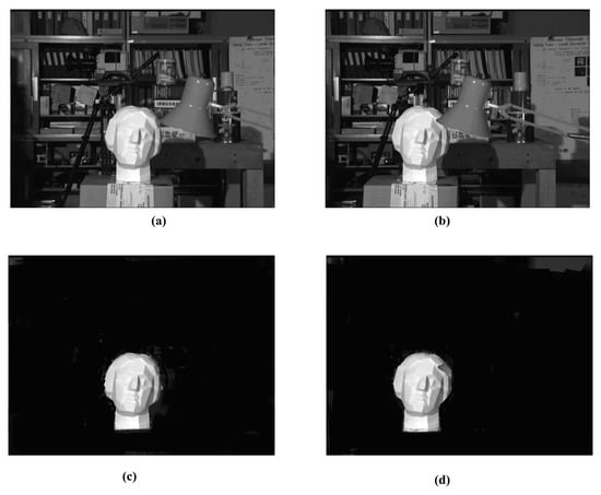
Figure 8.
The reconstruction outcomes for real-world stereo imagery are illustrated as follows: (a,b) the Tsukuba stereo image pair; (c,d) the segmented regions corresponding to the objects of interest.
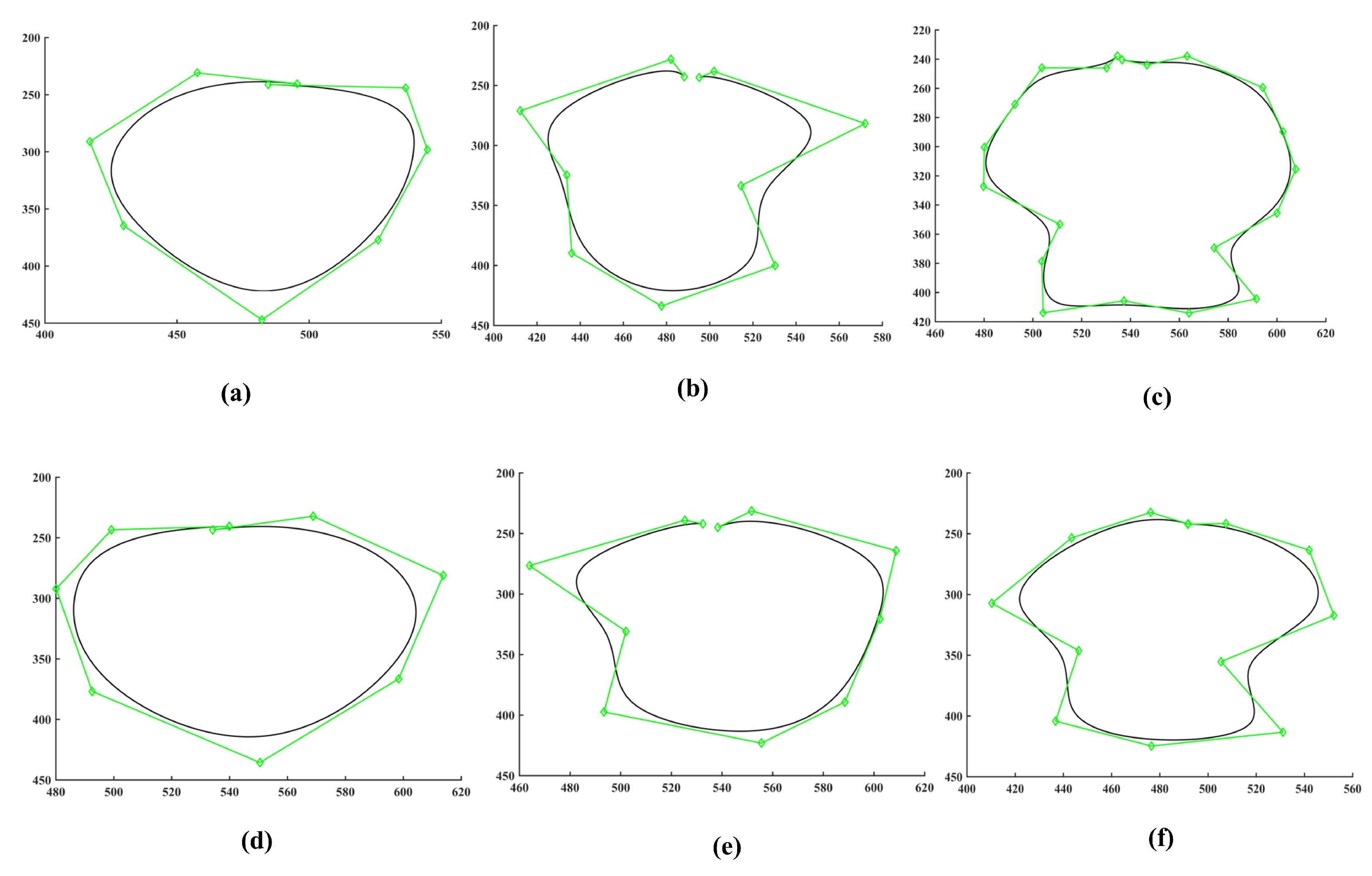
Figure 9a–c show the fitting results in one plane obtained using the described iterative fitting procedure, while Figure 9d–f show the fitting results in another plane. Figure 10a–c show the reconstruction results produced in each scenario, demonstrating how well the suggested technique performs on a real dataset. Figure 10a displays the result with nine evolved control points, which is neither accurate nor representative of the actual set of boundaries. Figure 10b, which shows the result with the 13 control points, resembles the actual frame, but it is not as accurate as the results presented previously in [16,19]. Continuing the iterative reconstruction process, the final result is presented in Figure 10b with 20 control points that outperform the previous methods.
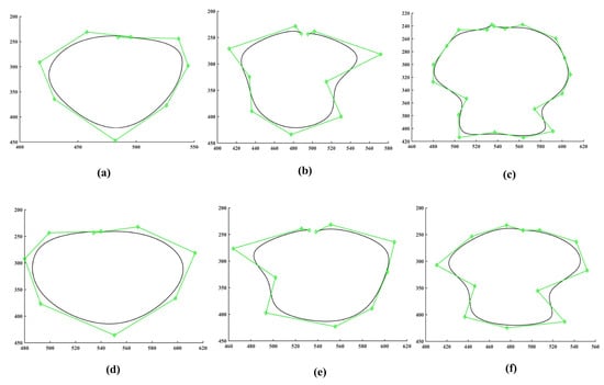
Figure 9.
Reconstruction outcomes for stereo image data are depicted as follows: (a,d) curve fitting in the left and right views using 9 control points; (b,e) corresponding fits with 13 control points; (c,f) results obtained using 20 control points in both views.
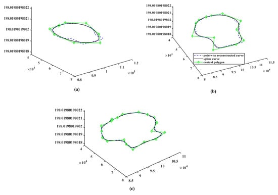
Figure 10.
Reconstruction performance on real stereo imagery is illustrated as follows: (a) result obtained using 9 control points; (b) reconstruction using 13 control points; (c) output with 20 control points.
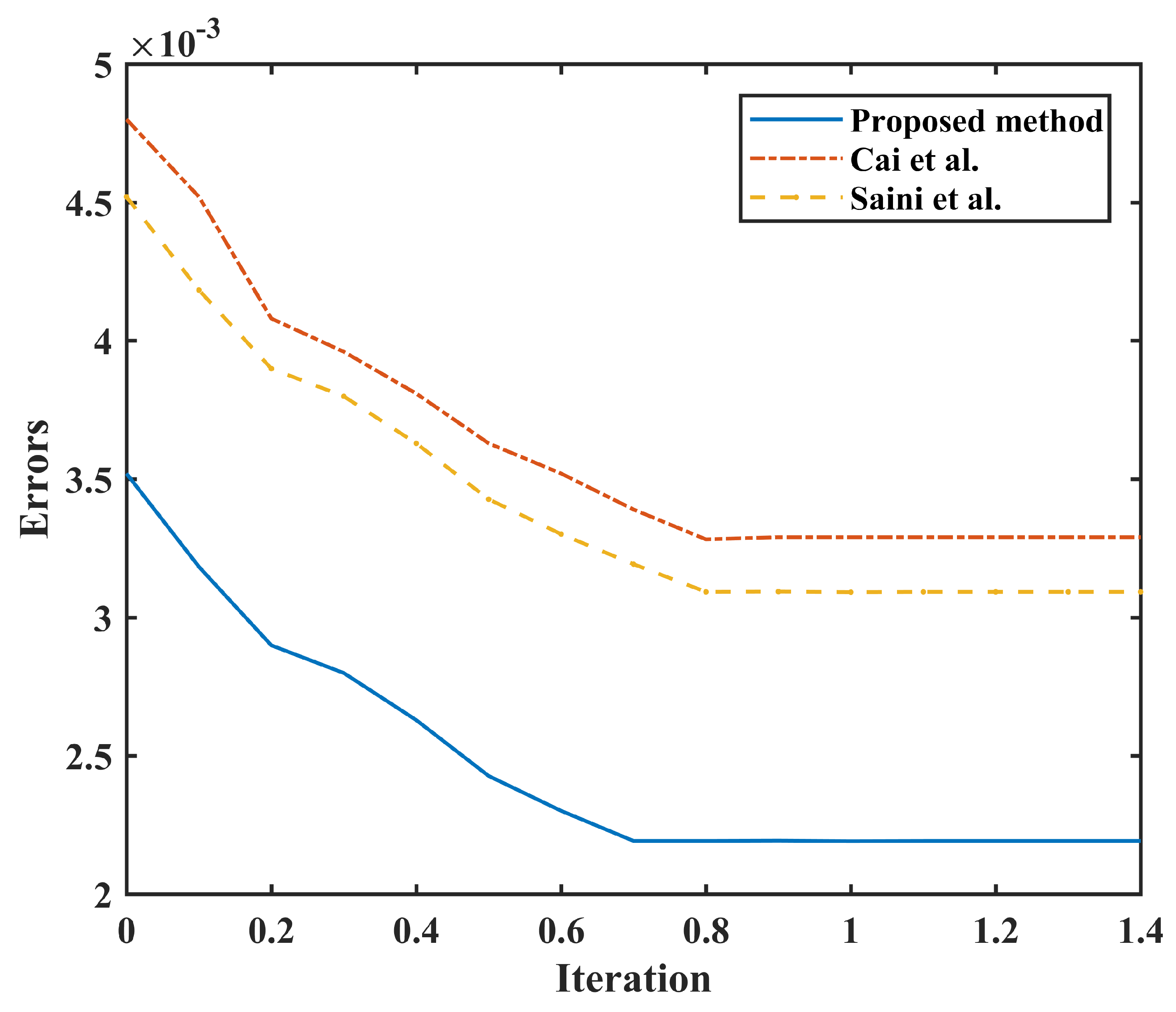
To assess the reliability of the proposed approach, its performance is evaluated against that of other existing iterative techniques, including those proposed in [19,20]. The convergence plot is plotted as a function of iteration vs. average errors and is shown in Figure 11. In this graph, it is observed that errors decrease faster compared to the other two methods [19,20].
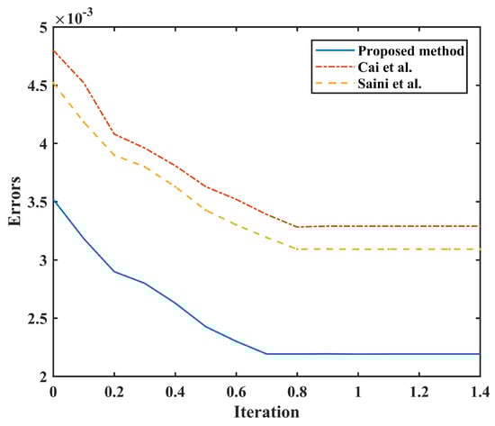
Figure 11.
Comparison result of the convergence plots of different approaches [19,20].
To further validate the proposed framework, we compare its reconstruction performance with several recent techniques beyond the traditional NURBS-Snake [20] and point-based [17] models. Specifically, we benchmark our approach against the least-squares progressive iterative approximation (LSPIA) method [7] and knot optimization using sparse representation [9]. These newer models offer improvements in local control or efficiency but struggle with noisy or complex datasets. In contrast, our method consistently exhibits faster convergence, greater shape fidelity, and lower sensitivity to initial configurations, as supported by error metrics (Table 1) and statistical tests (Table 2, Table 3, Table 4 and Table 5). The combined optimization of weights and parameters within a unified energy framework offers a significant advantage in practical deployments.
Table 2.
Mean errors under different noise levels.
Table 3.
Standard deviation of errors under the different noise levels.
Table 4.
F-test statistical analysis under noisy conditions.
Table 5.
t-test statistical analysis under noisy conditions.
The proposed iterative algorithm was implemented in MATLAB R2019 and tested on a machine with a 2.53 GHz Intel i3 processor and 3.0 GB RAM. Despite its iterative nature, the optimization converged in 10 to 25 iterations for most datasets, consuming approximately 12 to 18 s for moderately sized curves (up to 50 control points). The memory footprint remained under 150 MB, as the dominant operations involved matrix construction and singular value decomposition (SVD), which are efficiently handled in MATLAB. This lightweight computational profile highlights the suitability of the proposed method for real-time or embedded applications with limited resources. Empirically, the runtime grew linearly with the number of iterations and control points due to matrix assembly and SVD computation. The modular optimization structure ensures that the time complexity per iteration remains manageable (, where m is the number of control points and n is the number of data samples). The method remains computationally feasible for real-world datasets, demonstrating scalability and efficiency under moderate hardware settings.
4. Statistical Analysis
In this investigation, the accuracy of curve reconstruction was quantitatively evaluated using statistical descriptors—namely, the mean and standard deviation of error metrics—computed between the reconstructed and original curves. A benchmark parametric curve defined by was employed as the test function. The statistical outcomes for this dataset, including mean and standard deviation values, are summarized in Table 2 and Table 3. The proposed reconstruction framework was comparatively assessed against the stereo point-based method [17] and the NURBS-Snake method [20] under varying noise intensities. The results in both tables consistently indicate that our method yields lower reconstruction errors. To validate the statistical significance of these improvements, we conducted a comprehensive analysis using both F-tests and two-tailed t-tests.
4.1. F-Test
To determine whether the variability in reconstruction outcomes remained stable across different noise levels, a two-tailed F-test for equality of variances was conducted at the significance level (). The test compared the variance values derived from multiple datasets, each subjected to different noise intensities. The corresponding F-statistic values, summarized in Table 4, were found to be within the critical interval defined by the F-distribution bounds, i.e., at degrees of freedom.
As all the computed F-statistic values fell within this acceptance region, the null hypothesis that the population variances are equal could not be rejected for any of the datasets. This confirms that the variability in reconstruction accuracy introduced by noise did not differ significantly across methods, validating the assumption of homoscedasticity.
Accepting the equal-variance assumption is crucial for the reliability of subsequent t-tests comparing reconstruction accuracy, as it ensures that the statistical inferences are based on valid premises. Moreover, the consistency of variance across noise levels also reflects the robustness of the proposed method under perturbations, supporting its suitability for practical applications where noise is often unavoidable. This statistical stability complements the previously demonstrated accuracy benefits, reinforcing the overall effectiveness of the method.
4.2. t-Test
Subsequently, two-tailed t-tests (equal variances, ) compared the proposed method with the point-based reconstruction approach [17]. The t-statistic values (Table 5) exceeded the critical threshold (1.9799) for all noise levels, rejecting the null hypothesis. This statistically significant difference () demonstrates the superior precision of our method over the NURBS-Snake technique [20]. The results indicate that the proposed approach produces significantly better reconstruction accuracy, even at varying levels of random noise contamination. By integrating control-point optimization, weight adjustment, and iterative refinement through energy minimization, the method effectively addresses limitations observed in earlier techniques, such as the NURBS-Snake model. The consistent statistical advantage across multiple test scenarios highlights not only the robustness but also the adaptability of our framework to noisy real-world data.
These findings underscore the potential of the method for practical applications where high-fidelity curve reconstruction is required, particularly in environments where noise and sampling irregularities are common. The statistically validated performance improvement further supports the use of this approach as a reliable alternative to existing reconstruction methods.
5. Conclusions
This study introduces a method to accurately reconstruct space curves by optimizing certain data parameters using a mathematical model called Nonuniform Rational B-Splines (NURBSs). NURBSs are widely used in computer graphics and geometric modeling because they can represent complex shapes smoothly and precisely. The key idea in this method is to fine-tune the “weights” of the NURBSs, which play a big role in shaping the curve.
Instead of adjusting everything at once, the method makes gradual changes to these weights over several steps. This step-by-step process helps to better match the curve to the original data points, even when the data contain some noise or inaccuracies. To make these adjustments efficient and reliable, a simplified mathematical approach is used that involves linear approximation and nonlinear optimization. This makes it possible to find the best possible weight values without requiring overly complex calculations.
This paper also provides a clear explanation of the entire iterative and fitting reconstruction process. To test how well it works, we conducted a series of numerical experiments. These tests resulted in the finding that the proposed technique is not only more accurate in reconstructing curves but also more resistant to noisy or imperfect data compared to previous methods that use similar optimization strategies.
The proposed framework, built on the NURBS framework, already a core component in CAD environments, can be seamlessly integrated into commercial software such as AutoCAD, MicroStation, or Rhino. The optimized weight and parameter estimation algorithm can enhance curve refinement modules in such platforms, particularly for tasks involving reverse engineering or curve fitting from scanned or stereo-imaged data. Future work includes the development of plug-in modules that interface with CAD APIs to enable direct import of reconstructed 3D NURBS curves.
Author Contributions
Conceptualization, D.S. and S.K.; methodology, D.S. and S.K.; software, M.A., D.S. and S.K.; validation, M.A., D.S., S.K. and A.R.W.S.; formal analysis, M.A., S.K. and D.S.; investigation, M.A., D.S., S.K. and A.R.W.S.; resources, M.A., D.S. and S.K.; data curation, D.S. and S.K.; writing—original draft preparation, M.A., D.S. and S.K.; writing—review and editing, M.A., D.S., S.K. and A.R.W.S.; visualization, M.A., D.S., S.K. and A.R.W.S.; supervision, D.S. and S.K.; project administration, M.A.; funding acquisition, M.A. and A.R.W.S. All authors have read and agreed to the published version of the manuscript.
Funding
This work was supported by the Deanship of Scientific Research, Vice Presidency for Graduate Studies and Scientific Research, King Faisal University, Saudi Arabia [Grant No. KFU252542].
Data Availability Statement
The raw data supporting the conclusions of this article will be made available by the authors on request.
Conflicts of Interest
The authors assert that they have no conflicts of interest.
References
- Piegl, L.; Tiller, W. The NURBS Book; Springer Science & Business Media: Berlin/Heidelberg, Germany, 2012. [Google Scholar]
- Liu, C.; Liu, Z. Progressive iterative approximation with preconditioners. Mathematics 2020, 8, 1503. [Google Scholar] [CrossRef]
- Chang, Q.; Ma, W.; Deng, C. Constrained least square progressive and iterative approximation (CLSPIA) for B-spline curve and surface fitting. Vis. Comput. 2024, 40, 4427–4439. [Google Scholar] [CrossRef]
- Ma, W.; Kruth, J.P. Parameterization of randomly measured points for least squares fitting of B-spline curves and surfaces. Comput.-Aided Des. 1995, 27, 663–675. [Google Scholar] [CrossRef]
- Ma, W.; Kruth, J.P. NURBS curve and surface fitting for reverse engineering. Int. J. Adv. Manuf. Technol. 1998, 14, 918–927. [Google Scholar] [CrossRef]
- Jing, Z.; Shaowei, F.; Hanguo, C. Optimized NURBS curve and surface fitting using simulated annealing. In Proceedings of the 2009 Second International Symposium on Computational Intelligence and Design, Changsha, China, 12–14 December 2009; Volume 2, pp. 324–329. [Google Scholar]
- Zhang, M.; Li, Y.; Deng, C. Optimizing NURBS curves fitting by least squares progressive and iterative approximation. J.-Comput.-Aided Des. Comput. Graph. 2020, 32, 568–574. [Google Scholar]
- Dung, V.T.; Tjahjowidodo, T. A direct method to solve optimal knots of B-spline curves: An application for non-uniform B-spline curves fitting. PLoS ONE 2017, 12, e0173857. [Google Scholar] [CrossRef] [PubMed]
- Kang, H.; Chen, F.; Li, Y.; Deng, J.; Yang, Z. Knot calculation for spline fitting via sparse optimization. Comput.-Aided Des. 2015, 58, 179–188. [Google Scholar] [CrossRef]
- Laube, P.; Franz, M.O.; Umlauf, G. Learnt knot placement in B-spline curve approximation using support vector machines. Comput. Aided Geom. Des. 2018, 62, 104–116. [Google Scholar] [CrossRef]
- Ülker, E. B-Spline curve approximation using Pareto envelope-based selection algorithm-PESA. Int. J. Comput. Commun. Eng. 2013, 2, 60. [Google Scholar] [CrossRef]
- Tongur, V.; Ülker, E. B-spline curve knot estimation by using niched pareto genetic algorithm (npga). In Proceedings of the Intelligent and Evolutionary Systems: The 19th Asia Pacific Symposium, IES 2015, Bangkok, Thailand, 22–25 November 2015; pp. 305–316. [Google Scholar]
- Aguilar, E.; Elizalde, H.; Cárdenas, D.; Probst, O.; Marzocca, P.; Ramirez-Mendoza, R.A. An adaptive curvature-guided approach for the knot-placement problem in fitted splines. J. Comput. Inf. Sci. Eng. 2018, 18, 041013. [Google Scholar] [CrossRef]
- Conti, C.; Morandi, R.; Rabut, C.; Sestini, A. Cubic spline data reduction choosing the knots from a third derivative criterion. Numer. Algorithms 2001, 28, 45–61. [Google Scholar] [CrossRef]
- Tjahjowidodo, T.; Dung, V.; Han, M. A fast non-uniform knots placement method for B-spline fitting. In Proceedings of the 2015 IEEE International Conference on Advanced Intelligent Mechatronics (AIM), Busan, Republic of Korea, 7–11 July 2015; pp. 1490–1495. [Google Scholar]
- Deepika, S.; Sanjeev, K.; Gulati, T. NURBS-Based Geometric Inverse Reconstruction of Free-Form Shaped Objects. JKSU-Comput. Inf. Sci. 2014, 29, 116–133. [Google Scholar]
- Xiao, Y.J.; Li, Y. Optimized stereo reconstruction of free-form space curves based on a nonuniform rational B-spline model. J. Opt. Soc. Am. A 2005, 22, 1746–1762. [Google Scholar] [CrossRef] [PubMed]
- Piegl, L.A.; Tiller, W. Surface approximation to scanned data. Vis. Comput. 2000, 16, 386–395. [Google Scholar] [CrossRef]
- Cai, Y.; Su, Z.; Li, Z.; Sun, R.; Liu, X.; Zhao, Y. Two-view curve reconstruction based on the snake model. J. Comput. Appl. Math. 2011, 236, 631–639. [Google Scholar] [CrossRef]
- Saini, D.; Kumar, S.; Gulati, T.R. Reconstruction of free-form space curves using NURBS-snakes and a quadratic programming approach. Comput. Aided Geom. Des. 2015, 33, 30–45. [Google Scholar] [CrossRef]
- Wang, T.R.; Liu, N.; Yuan, L.; Wang, K.X.; Sheng, X.J. Iterative least square optimization for the weights of NURBS curve. Math. Probl. Eng. 2022, 2022, 5690564. [Google Scholar] [CrossRef]
- Hansen, P.C. The truncated SVD as a method for regularization. BIT Numer. Math. 1987, 27, 534–553. [Google Scholar] [CrossRef]

Disclaimer/Publisher’s Note: The statements, opinions and data contained in all publications are solely those of the individual author(s) and contributor(s) and not of MDPI and/or the editor(s). MDPI and/or the editor(s) disclaim responsibility for any injury to people or property resulting from any ideas, methods, instructions or products referred to in the content. |
© 2025 by the authors. Licensee MDPI, Basel, Switzerland. This article is an open access article distributed under the terms and conditions of the Creative Commons Attribution (CC BY) license (https://creativecommons.org/licenses/by/4.0/).