Abstract
The purpose of this paper is to present a novel optimization framework that enhances Wasserstein Distributionally Robust Optimization (WDRO) for chance-constrained facility location problems under demand uncertainty. Traditional methods often rely on predefined probability distributions, limiting their flexibility in adapting to real-world demand fluctuations. To overcome this limitation, the proposed approach integrates two methodologies, specifically a Genetic Algorithm to search for the optimal decision about facility opening, inventory, and allocation, and a constrained Jordan–Kinderlehrer–Otto (cJKO) scheme for dealing with robustness in the objective function and chance-constraint with respect to possible unknown fluctuations in demand. Precisely, cJKO is used to construct Wasserstein ambiguity sets around empirical demand distributions (historical data) to achieve robustness. As a result, computational experiments demonstrate that the proposed hybrid approach achieves over 90% demand satisfaction with limited violations of probabilistic constraints across various demand scenarios. The method effectively balances operational cost efficiency with robustness, showing superior performance in handling demand uncertainty compared to traditional approaches.
Keywords:
constrained JKO (cJKO); chance-constrained optimization; Wasserstein distance; facility location; Genetic Algorithm (GA) MSC:
90C17
1. Introduction
Supply chain management (SCM) is critical in modern logistics and resource allocation. With the rise of the sharing economy, supply chains are becoming more decentralized, flexible, and demand driven. In the era of global uncertainty and volatile markets, supply chain networks are increasingly exposed to risks stemming from unpredictable factors such as demand fluctuations, global disruptions (e.g., COVID-19), geopolitical risks, and operational variability [1]. If not properly addressed, these uncertainties lead to inventory imbalances, excess operational costs, and reduced service levels.
The location of a facility (FLP) is a classical subject area in combinatorial optimization with wide applications ranging from communication systems to supply chain planning, public services, and economic development. FLP occurs in various real applications like the location of logistical centers, industrial estates, gas filling stations, communication base stations, and other essential infrastructures such as hospitals, schools, supermarkets, and warehouses [2]. Despite its extensive use, classical FLP models usually assume deterministic conditions that do not reflect the intrinsic uncertainties characterizing real-world systems. Consequently, the obtained solutions are brittle and not optimal when subjected to real-time variations. To build robust and affordable supply chains, uncertainty must be integrated directly within both the framework of modeling and optimization. Among all the different kinds of uncertainty, demand uncertainty is especially significant since it has direct effects on capacity planning, inventory, and service fulfillments. Tackling this uncertainty has become a major challenge in the fields of operations research, decision science, and machine learning. Several methodological paradigms have emerged to address this issue, each grounded in different assumptions about the availability and structure of data—ranging from classical stochastic optimization to robust and distributionally robust approaches.
A standard approach to addressing uncertainty in optimization is Stochastic Optimization (SO), where decision-making is based on an assumed known probability distribution of demand. However, the true demand distribution is unknown, and only historical data (empirical distribution) are available. To model this uncertainty, distributionally robust optimization (DRO) has emerged as a powerful technique. Unlike traditional stochastic methods based on sample average approximation (SAA) optimization, DRO considers an ambiguity set of possible distributions instead of assuming a single known distribution. Table 1 presents three key optimization paradigms—SO, Worst-Case Robust Optimization (RO), and DRO—and their respective mathematical formulations.

Table 1.
Different optimization objectives considered in Bayesian optimization.
In this paper, the uncertain parameter is the customer’s demand, that is, a I-dimensional vector with I the number of customers. Thus, a scenario is represented by one demand vector and a set of scenarios—for instance, a historical dataset—can be viewed as a point clouds, namely, an empirical multivariate distribution capturing the inherent fluctuations in customer behavior due to external factors such as market trends and disruptions.
Given these fluctuations, it is crucial to develop robust facility location and allocation strategies that remain effective under a wide range of possible future demands. To this end, we address the distributionally robust facility location problem under demand uncertainty, where the true demand distribution is unknown and only sample-based approximations are available. Instead of relying on a single known distribution, we propose a Wasserstein Distributionally Robust Optimization (WDRO) framework, which defines an ambiguity set (aka Wasserstein ball) of plausible distributions around historical data.
The Wasserstein distance is rooted in optimal transport theory [3,4,5] and provides a mathematically rigorous and flexible measure of difference between distributions, making it particularly well-suited for constructing ambiguity sets in data-driven settings. Its usefulness has been recently reported, for instance, in the optimization of composite functions [6].
We formulate a joint optimization problem that determines
- (i)
- facility opening decisions,
- (ii)
- inventory levels, and
- (iii)
- customer allocations,
with the goal of minimizing the total supply chain cost, including fixed facility costs, inventory holding costs, transportation costs, and penalties for unmet demand, while satisfying demand with high probability.
To efficiently solve this complex and high-dimensional problem, we use a Genetic Algorithm (GA) to heuristically generate solutions for both discrete and continuous decision variables. Furthermore, we integrate a constrained Jordan–Kinderlehrer–Otto (cJKO) scheme, originally presented in [7]. Unlike standard JKO methods, cJKO provides a more effective and efficient mechanism for solving optimization problems over a space of probability distributions equipped with the Wasserstein distance.
The resulting hybrid metaheuristic-variational framework enables the effective exploration of the combinatorial decision space and robust handling of distributional uncertainty. By leveraging the Wasserstein distance, our model balances adaptability and robustness, avoiding overfitting to historical data while remaining responsive to dynamic demand shifts. Overall, this integrated approach ensures that facility placement and resource allocation remain cost-effective and resilient. The iterative cJKO updates allow for the dynamic refinement of uncertainty sets, improving the solution quality over time. Our method provides a scalable and theoretically grounded solution for optimizing supply chain operations under deep uncertainty.
The remainder of this paper is structured as follows: Section 2 reviews the relevant literature, highlighting the applications of stochastic optimization, robust optimization, and distributionally robust optimization in facility location problems. Section 3 presents the problem statement, formally defining the optimization problem. In Section 4, we introduce the approach of optimizing over probability distributions, discussing how uncertainty is incorporated into the decision-making process. Also, this section describes the metaheuristic-based approach used to efficiently solve the problem, highlighting its advantages. In Section 5, we provide computational results, demonstrating the performance of our proposed methodology through extensive numerical experiments. Finally, Section 6 concludes the paper by summarizing the key findings and outlining potential directions for future research.
2. Literature Review
Facility location problems under uncertainty have long been a central theme in operations research and supply chain design [8]. Classical approaches often rely on deterministic formulations, assuming perfect knowledge of input parameters such as demand and transportation costs [9]. However, real-world supply chains are increasingly impacted by volatile customer demand, supply disruptions, and economic shifts. To address these challenges, several optimization paradigms have been proposed, each with distinct assumptions and trade-offs. In this section, we review the literature surrounding these approaches and their application to facility location problems, with a focus on recent advances incorporating Wasserstein-based DRO models and metaheuristic strategies.
2.1. Stochastic Optimization in Facility Location
SO aims to maximize the expected performance of a decision x under a fixed probability distribution P of the uncertain parameter c (Formula (1)). This approach assumes that P is known in advance or can be estimated reliably from historical data.
SO has been extensively applied to facility location problems where demand or cost parameters are modelled as random variables with known probability distributions. Classical SO methods aim to minimize the expected cost by solving a two-stage or multi-stage model. In the first stage, strategic decisions such as facility openings are made, while in the second stage, recourse actions, including allocations or inventory replenishments, are optimized based on the realization of uncertainty. Works such as those by Snyder [10] and Laporte et al. [11] provide foundational methodologies for modeling uncertainty in facility location through scenario-based planning.
However, one major limitation of SO lies in its reliance on the accuracy of the assumed probability distribution, which is often derived from historical or simulated data. In real-world applications, these distributions may not accurately reflect future conditions due to dynamic market trends, policy changes, or unforeseen disruptions. As a result, solutions based on SO can become suboptimal or even infeasible when the actual demand distribution deviates from the expected one. This sensitivity to distributional misspecification can undermine the robustness of the decisions derived from SO models. Nevertheless, SO remains a widely used and valuable benchmark approach in the facility location literature and has been successfully applied to various settings, including capacitated facility location problems, multi-period planning, and emergency service deployment.
2.2. Robust Optimization in Facility Location
RO takes a conservative approach by optimizing for the worst possible realization of the uncertain parameter c within a predefined set Δ (Formula (2)). The goal is to ensure that the decision x performs well even under the most adverse conditions. This approach is particularly useful in safety-critical applications, such as finance and healthcare, where extreme scenarios must be accounted for.
RO offers an alternative approach by eschewing probabilistic information in favor of worst-case guarantees. The underlying philosophy of RO is to optimize decisions that perform acceptably under all realizations of uncertainty within a predefined uncertainty set. Kouvelis and Yu [12] were among the early pioneers in introducing RO into supply chain planning, and their work was followed by many others who sought to build resilient networks without requiring probabilistic information.
RO has been extensively applied in the facility location literature to ensure system performance under extreme or adversarial demand scenarios. For instance, Jabbarzadeh et al. [13] proposed a robust location allocation model for humanitarian supply chains that guarantees network resilience even under the most disruptive conditions. Despite its effectiveness in providing high levels of reliability, RO tends to be overly conservative. By focusing solely on worst-case scenarios, it often neglects probabilistic information about more likely demand realizations. This leads to overly cautious solutions that can result in excessive costs under normal operating conditions. Furthermore, RO does not fully exploit valuable insights derived from empirical data, potentially missing opportunities to achieve a more balanced trade-off between cost-efficiency and robustness.
2.3. DRO in Facility Location
DRO provides a middle ground between SO and RO by considering uncertainty in the probability distribution itself. Instead of assuming that the context c follows a fixed distribution P, DRO optimizes for the worst-case expectation over all distributions Q within an uncertainty set U [14] (Formula (3)). This makes DRO highly effective in environments where the true distribution is unknown or subject to shift. The uncertainty set U is often defined using divergence measures, such as the Wasserstein distance, φ-divergences, or Maximum Mean Discrepancy (MMD) [15]. DRO has gained significant attention due to its ability to account for distributional shifts while avoiding the extreme conservatism of RO [16]. It has applications in robust machine learning models, adversarial training, reinforcement learning, and optimization problems under uncertainty. In the context of Bayesian optimization, adopting a DRO-based approach can significantly improve model robustness [17], particularly in non-stationary environments where data distributions change over time [18]. By selecting the appropriate optimization paradigm based on the problem’s uncertainty characteristics, decision-makers can better balance performance and robustness in their optimization tasks.
Many studies have explored DRO in facility location, often using moment-based or φ-divergence-based ambiguity sets. For example, Liu et al. [19] formulated a DRO model for emergency medical service station location using joint chance constraints. Their model ensured service reliability by optimizing over all distributions sharing known first- and second-order moments. More flexible are Wasserstein-based ambiguity sets, which define the uncertainty set using optimal transport metrics. Ji and Lejeune [20] applied Wasserstein DRO to chance-constrained facility location, demonstrating superior robustness and computational tractability. These models can incorporate empirical distributions (i.e., point clouds) and adapt to various demand scenarios, making them particularly effective for supply chain applications.
Wasserstein-based DRO has gained prominence due to its intuitive geometric interpretation, tractable reformulations, and strong theoretical guarantees. It measures the cost of transporting probability mass between distributions, naturally aligning with the logistics and spatial nature of facility location problems. Wang et al. [21] applied Wasserstein DRO to disaster relief logistics, modeling joint chance constraints under data-driven uncertainty.
Their results showed improved service levels and robustness under distributional shifts. Recent developments in Wasserstein DRO have focused on computational efficiency and scalability challenges: Ref. [22] provided a comprehensive duality framework for Wasserstein DRO that offers more efficient reformulations, while advances in statistical distance-based DRO algorithms have addressed computational complexity in large-scale scenarios through decomposition and approximation techniques.
2.4. Types of Ambiguity Sets in DRO
Before constructing a DRO model, it is crucial to define how the uncertainty about the true distribution is represented. While SO assumes a known distribution and RO operates without any probabilistic assumptions, DRO acknowledges distributional uncertainty—the fact that the true probability distribution is only partially known. This uncertainty is formalized through an ambiguity set, a collection of distributions deemed plausible based on the available data, prior knowledge, or statistical properties. The DRO model then seeks to optimize performance under the worst-case distribution within this ambiguity set. As such, the construction of the ambiguity set plays a central role in balancing robustness and conservatism, influencing both the theoretical properties and empirical outcomes of the solution.
Ambiguity sets can be constructed based on different principles:
- Moment-based ambiguity sets—constraints on mean, variance, and higher moments [16];
- Discrepancy-based ambiguity sets—define a neighborhood of plausible distributions around a reference measure (e.g., Kullback–Leibler divergence and total variation distance) [23];
- Wasserstein-based ambiguity sets—a natural and flexible framework using the Wasserstein metric to measure the distance between distributions [24,25].
Among these, the Wasserstein-based ambiguity set has recently gained dominance due to its mathematical/statistical background. The Wasserstein distance measures the cost of transporting probability mass between distributions. This makes it highly suitable for supply chain applications, where demand fluctuations can be viewed as shifts of empirical distributions (i.e., set of historical demand data) within a neighborhood of a certain Wasserstein radius.
2.5. Computational Trade-Offs in Distributionally Robust Facility Location
The computational complexity of DRO-based facility location models presents significant challenges that must be carefully balanced against solution quality and robustness benefits. Unlike traditional stochastic optimization, which deals with a fixed probability distribution, DRO requires optimization over an entire ambiguity set, fundamentally increasing the problem’s computational burden. The primary computational challenges arise from the need to solve min-max optimization problems, where the inner maximization over the ambiguity set often leads to semi-definite programming reformulations or requires sophisticated duality theory [26]. In facility location contexts, this complexity is compounded by the discrete nature of location decisions and the continuous nature of allocation variables, creating mixed-integer optimization problems that are inherently difficult to solve. While Wasserstein-based ambiguity sets offer intuitive geometric interpretations and strong theoretical guarantees, they come with higher computational costs compared to moment-based or φ-divergence approaches. The state-of-the-art methods for Wasserstein DRO rely on global optimization techniques, which quickly become computationally prohibitive for large-scale problems [25]. However, recent algorithmic advances have improved tractability through efficient reformulations and decomposition strategies. Practitioners must balance between problem size, solution time, and robustness level. Larger ambiguity sets provide greater distributional robustness but exponentially increase the computational requirements. Effective scenario identification techniques can reduce this computational burden by focusing on scenarios that most significantly impact the optimal solution [26].
2.6. Metaheuristic Approaches and Genetic Algorithms in Facility Location
Given the combinatorial complexity of facility location problems, especially under uncertainty, exact algorithms often struggle to scale. Metaheuristic methods such as Genetic Algorithms (GAs), Simulated Annealing (SA), and Particle Swarm Optimization (PSO) have been widely adopted to overcome these limitations. GAs are particularly well-suited for mixed-integer optimization problems thanks to its ability to explore large and nonlinear search spaces efficiently [27].
In recent years, hybrid models combining GAs with SO or RO have emerged. Saeedi et al. [28] developed a two-stage stochastic programming model for a closed-loop Electric Vehicle (EV) battery supply chain under demand uncertainty. They used meta-heuristic algorithms to optimize facility location and inventory decisions, encoding key variables into chromosomes.
By integrating a GA with WDRO, this work combines the global search strengths of meta-heuristics with the rigor of modern DRO. The incorporation of the cJKO scheme enables the dynamic evolution of Wasserstein ambiguity sets alongside decision updates, resulting in adaptive and resilient solutions under demand uncertainty.
2.7. Optimization of Probability Distributions
The standard JKO scheme is a variational formulation originally developed to solve gradient flows in the space of probability measures [7]. Recent research has adapted this scheme to solve optimization problems over distributions, notably in Bayesian optimization and physics-informed learning [29]. The constrained JKO (cJKO) variant enforces an upper bound on the Wasserstein distance between iterations, offering a principled way to control distributional shifts and update empirical distributions while preserving proximity to the observed data [30]. Although applications of cJKO in supply chain optimization are nascent, its potential is significant. Our work is among the first to apply the cJKO scheme to distributionally robust facility location under chance constraints.
3. Problem Statement
In supply chain management, uncertainty plays a crucial role in decision-making. Classical deterministic models assume that the demand is perfectly known, but real-world scenarios involve an uncertain demand due to market fluctuations, economic factors, and unpredictable customer behavior. To tackle demand uncertainty, we adopt a WDRO framework, that is, DRO with a Wasserstein-based ambiguity set. The goal is to minimize supply chain costs while ensuring robust facility, storage, and allocation decisions. Table 2 presents the notations used throughout this paper, defining the indices, parameters, and decision variables essential for formulating the optimization model.
Table 2.
Notations.
Problem Formulation
In the supply chain optimization model, the primary decisions to be made include (1) facility location decisions, which determine whether facility j should be opened in period t, represented by the binary variable ; (2) inventory management decisions, where the inventory level at facility j in period t, denoted by , is optimized to adjust storage levels in response to fluctuating demand while minimizing holding costs; and (3) transportation and allocation decisions, where the quantity is transported from facility j to customer i in period t, aiming to minimize transportation costs while fulfilling customer demand . Without loss of generality, the demand of each customer is considered fixed over time (i.e., it does not depend on t).
Decisions must be taken under demand uncertainty and are designed to minimize total supply chain costs while maintaining operational efficiency. The objective function of the reference problem consists in minimizing the total cost associated with facility location and allocation under demand uncertainty. It consists of two terms:
- (i)
- Facility operation costs, represented by fixed opening costs and inventory holding costs , ensure that storage levels adjust optimally over time. This term is “deterministic” in the sense that its computation does not depend directly on the demand and its uncertainty.
- (ii)
- Transportation and allocation costs are captured through expected costs over the unknown probability distribution , including demand-dependent shipping costs and penalties related to supply shortages. This term depends directly on the demand and its uncertainty; indeed, it is a penalization with respect to unmatched demand due to fluctuations. Its computation requires finding the worst-demand possible P, meaning to solve an optimization problem over probability distributions, specifically a Wasserstein neighborhood of the historical data.
The optimization of the objective function (4) is subject to the following constraints:
Chance Constraint for Demand Satisfaction
Facility and Allocation Constraints
Allocation Constraint
Facility and Capacity Constraints
The chance constraint for demand satisfaction (5) guarantees that the probability of supply shortages remains below a predefined threshold , improving reliability. Analogously to the objective function, the computation of (5) requires solving an optimization problem over probability distributions, meaning that cJKO will be used to compute the left-hand side term of the inequality in (5).
Facility operation constraints (6) enforce binary decisions for facility openings and nonnegative allocations. The allocation constraint (7) ensures that each demand node receives an appropriate share of the supply without exceeding the available capacity. Finally, capacity constraints (8) limit inventory levels based on facility availability, ensuring that stored goods do not exceed practical limits. These constraints collectively shape an efficient, resilient, and mathematically rigorous facility location model that effectively manages uncertainty and distributional shifts in demand.
Another important constraint is related to cJKO itself, rather the supply chain problem. Specifically, we must set at each iteration of the cJKO algorithm, where is the probability distribution at step k, P is the decision variable (i.e., probability distribution), and is the radius—in Wasserstein terms—of the ambiguity set (aka Wasserstein ball) around the current candidate solution . All the details about cJKO and are detailed in the next section.
4. Solution Approach
4.1. Optimizing over Probability Distributions
The computation of the objective function (4) and the probabilistic constraint (5) requires solving two optimization problems over distributions separately, that is, searching for the worst demand distribution affecting the objective value and the worst demand distribution affecting the demand satisfaction constraint.
Without loss of generality, we can consider the reference problem
where refers to a generic functional to be minimized over the space of probability measures . Solving problem (9) means searching for a sequence of probability distributions starting from an initial random guess (typically a multivariate Gaussian) and converging to . A well-known example for problem (9) is given in [7], showing that solving the Fokker–Planck PDE is equivalent to minimize an entropy functional over the space of probability measures, equipped with the so-called Wasserstein distance.
The Wasserstein distance is defined as the minimum cost for transporting probability density mass from a source probability density to match a target probability density, and where the cost is computed in terms of a distance (also known as the ground metric) between points of the support. In this paper, we consider the case that the cost is the Euclidean distance, leading to the so-called 2-Wasserstein distance:
where means that applying to (i.e., our source distribution) will obtain (i.e., our target distribution) as result. denotes the so-called push-forward operator; while is interpreted as a function moving a single data point (i.e., a customers demand scenario, in our case) over the support , represents its extension to an entire probability measure.
The Brenier Theorem [3,4] guarantees that the problem (10) has a unique optimal solution , named the optimal transport map. Furthermore, the Brenier theorem also states that the optimal transport is equal to the gradient of a convex function , such that .
By introducing a coefficient , we can define a continuous-time representation of the optimal transport map , that is,
Easily, the following discrete-time representation can be derived:
with and where is a discretization of . As a result, the sequence solves (10), with as the solution of (10).
Since is not known a priori, cannot be directly computed. A widely adopted method to solve (10) is the JKO (Jordan–Kinderlehrer–Otto) scheme [7] that is a proximal point method with respect to the 2-Wasserstein distance or, from another point of view, a backward Euler discretization. At a generic iteration , JKO transports the current probability density, , into the next according to
with as the JKO’s step size.
Solving problem (14) translates into searching for the next probability density that minimizes the functional within a 2-Wasserstein neighbourhood of the current , that is, a Wasserstein ball (aka ambiguity set) around . Iteratively solving problem (13) leads to a sequence whose rate of convergence to depends on : with , the first term goes to zero, meaning that we are minimizing but at the expense of obtaining a transport far away from the optimal one. On the contrary, if , then the first term becomes more relevant so that the generated sequence will be close to but it will converge significantly slowly to .
Finally, problem (9) is formulated in terms of , that is, having probability densities as decision variables. State-of-the-art approaches recast problem (9) as an optimization problem in terms of a parametrized transport map from to . For instance, the convex function is usually approximated through an Input Convex Neural Network (ICNN) [31,32,33], a specific type of Deep Neural Network (DNN), and then is obtained by following the Brenier Theorem, namely, . DNNs are also used in [34,35] to approximate through a DNN, whose output is then used as an input—along with —of another DNN estimating . Contrary to the ICNN-based approaches, this method allows for skipping the computation of . More recently, [36] proposed to parametrize through a Residual Neural Network (ResNet) and a variational formulation of the functional formulated as maximization over a parametric class of functions. This allows for reducing the computational burden with respect to the previous methods using small data samples and scaling well with the dimensionality of the support . The small data regime setting has been also recently investigated in [37], who proposed to combine OT solvers and Gaussian process regression to efficiently learn the transportation map. The most relevant issue for all the neural approaches is that at least one neural network must be trained, leading to relevant computational costs at each JKO step. Since getting close to requires and consequently a number of iterations , this issue becomes even more critical. Moreover, there are not specific guidelines on how to choose the most suitable neural network to use. Moreover, [38] has recently reported that normalizing flow models based on neural networks can only generate planar flows, which are proven to be expressive only in the case of univariate probability densities (i.e., 1-dimensional support). Another relevant study on the convergence and the self-consistency of normalizing flows in the space of probability density equipped with the Wasserstein distance is given in [39].
The Constrained JKO Schema
The parametrization of the transport plan considered in this paper has been originally proposed in [30], and is defined as follows:
with , and is a rotation matrix consisting of a sequence of matrix multiplications, , where is defined as
where denotes the th component of the vector-valued function .
Finally, is a reference versor; for simplicity, we consider , where denotes the all-ones vector and, therefore, .
From the Brenier theorem, we know that , and so we are posing . The parameters to be learned in the proposed parametrization are the two functions and . Contrary to the ICNN-based parametrizations, but analogously to [34,35,36], the proposed parametrization does not require any assumptions on the two functions to be learned.
According to the proposed parametrization, the JKO schema can be recast into
with .
Like all the other approaches, we learn the functions underlying our parametrization by accessing to point clouds (i.e., empirical distributions) sampled from probability densities [30]. Analogously to other neural networks-based approaches, denote with the point cloud at iteration obtained as
with such that . According to our parametrized transport , every point of the current cloud is transported as follows:
with and representing shorthand for and .
Since we are working with point clouds, and according to our parametrization, we can rewrite the 2-Wasserstein distance as follows:
Since rotation does not modify the module of the rotated v, and according to our choice for v, we have . Finally, we can write
with .
This allows us to set a threshold ε on the term to explicitly quantify the Wasserstein ball around the current , instead of weighting with respect to through the value of in the standard JKO schema.
Finally, the constrained-JKO (cJKO) scheme can be formalized:
with as a small positive quantity, , , and .
In simpler terms, we are searching for , which minimizes within a 2-Wasserstein neighbourhood of .
Indeed, in cJKO operates analogously to in JKO, requiring a longer sequence to converge to , but providing a transport close to the optimal one. However, it is important to clarify that, from a quantitative perspective, they are completely different. Since is just a scalarization weight into a scalarized bi-objective problem, it is quite impossible to establish a suitable value without any prior knowledge about . Furthermore, using a constant value for , which is the common choice, leads to a significantly different relevance of the two objectives over the JKO iteration
The cJKO scheme overcomes these limitations thanks to : it is chosen in advance and kept fixed along the overall iterative optimization process, independently on the values of over the iterations. Figure 1 shows an example of the trajectories from to depending on three different values of . The three presented cases converge to the same value of (and same final point cloud) but within a different number of cJKO steps: the smaller the value of ε, the larger the number of iterations K, and the closer the final transport to the optimal one (i.e., trajectories are closer to the actual , because they are more straight and do not overlap).
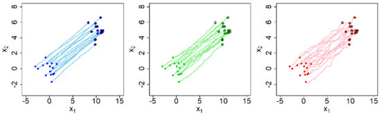
Figure 1.
Effects of on cJKO convergence and Wasserstein flow behavior [29].
As far as the application problem considered in this paper is concerned, cJKO is used to compute the second (stochastic) term of the objective function (4) and the chance constraint (5) separately, given a candidate solution for the facility location problem.
For completeness, we report the generic algorithm for the cJKO scheme, as follows. It is important to clarify that it is separately applied to identify the demand distributions—within an -radius Wasserstein ball of the historical demand data —providing (a) the maximum penalization in the objective function, that is, the second term in (4), and (b) the minimum probability in the chance constraint (5).
cJKO Algorithm for distributionally robust optimization
- Input:
- ○
- [X, S, Y] candidate solution (provided by the GA meta-heuristic);
- ○
- historical demand data;
- ○
- (i.e., cJKO’s parameter);
- ○
- (i.e., cJKO’s iterations);
- ○
- functional to be optimized (i.e., objective function’s term to be minimized in (4) and left-hand side term of the chance constraint to be maximized in (5), separately);
- Step 0: ;
- Step 1: solve the following problem;
- Step 2: ;
- Step 3: if , go to Step 1;
- Return .
Since the true probability distribution of the demand is unknown, as well as changes due to unpredictable events, it is difficult to define suitable values for and a priori. On the other way round, their values are easy to interpret: larger values increase robustness against events that could lead to demand values that are significantly different from the historical ones, but this means that the final decision might be too conservative. On the contrary, smallest values assume that the future demand should not change too much with respect to historical data, leading to less conservative decisions but difficulty in dealing with possible significant changes. The suggestion is to perform different runs with different values of and , with the aim to observe differences both in term of the final solution and generated demand distributions. Finally, the user can select the most suitable decisions (and scenario) for the specific goals of the target setting.
4.2. Metaheuristic-Based Approach
In this section, we introduce a metaheuristic optimization framework for distributionally robust supply chain design under demand uncertainty. Our approach integrates
- A Genetic Algorithm (GA) for the heuristic initialization of facility location, storage levels, and allocation decisions;
- The cJKO scheme to compute the stochastic term of the objective function (4) and the chance constraint (5) separately;
- A robust evaluation function that balances operational cost and risk-averse decision-making.
This hybrid method provides an efficient alternative to exact methods, particularly in high-dimensional settings, in which classical optimization techniques struggle with combinatorial complexity.
4.2.1. Genetic Algorithm for Heuristic Initialization
In step ①. to enhance the efficiency of the optimization process, we employ a GA for heuristic initialization. A GA is an evolutionary-based meta-heuristic that iteratively improves candidate solutions by mimicking natural selection principles, including selection, crossover, and mutation [40]. In our approach, the GA generates an initial population of facility location and allocation decisions, ensuring diversity in solutions while providing a high-quality starting point for subsequent optimization. By leveraging a GA, we improve the convergence speed and enhance the feasibility of the optimization model by reducing the likelihood of poor initializations. This approach is particularly beneficial for large-scale problems where a purely random initialization could lead to suboptimal or infeasible solutions.
Chromosome Representation
Every individual in the genetic population represents a possible supply chain configuration as a chromosome, encoding
- Facility location decisions ( binary matrix);
- Storage level decisions ( continuous matrix);
- Allocation decisions continuous matrix).
Formally, a chromosome is structured as chromosome = , where
- denotes whether facility j is open at time t;
- represents the storage level at facility j at time t;
- captures how much demand from the customer i is allocated from facility j at time t.
Fitness Function
The objective function in the genetic algorithm evaluates the total cost of a candidate supply chain configuration with Formula (4). It minimizes the sum of three key components: (i) fixed facility opening costs, (ii) inventory holding costs, and (iii) expected transportation costs and shortage penalties costs under stochastic demand while satisfying demand constraints.
Genetic Operators
The GA employs three main evolutionary operators:
- Selection (Tournament Selection);
- ○
- Randomly selects k-tournament competitors and chooses the best candidate.
- Crossover (Uniform Crossover);
- ○
- Swaps facility decisions and allocations between parent solutions to create diverse offspring. In this strategy, each gene (i.e., element of the chromosome representing facility decisions or allocations) is independently chosen from one of the two parent solutions with equal probability. This encourages greater diversity and exploration of the solution space by recombining building blocks from both parents.
- Mutation (Storage and Allocation Adjustment);
- ○
- Perturbs storage levels and allocations to introduce new feasible solutions. The swap mutation randomly selects two positions in the chromosome and exchanges their values. This perturbation helps the algorithm escape local optima by introducing structural variation into the solution while preserving feasibility.
- The GA runs for a predefined number of generations, yielding a near-optimal initial solution.
4.2.2. Wasserstein Distributionally Robustness via cJKO
Once an initial solution is generated in step ②, we use cJKO to compute the stochastic term of the objective function (4) and the chance constraint (5) separately.
Distributional Robustness via Wasserstein Distance. Starting from the point cloud associated with to historical demand, namely, , we iteratively search for to finally compute right term of the chance constraint (5).
cJKO Iterative Update Rule. At each iteration k, we solve the constrained Wasserstein optimization problem in Formulas (4) and (5). The process is repeated until a maximum number of iterations is reached. This ensures that our demand forecasts adapt dynamically based on historical and simulated uncertainty data.
4.2.3. Chance Constraint Verification ③
In supply chain and facility location problems, ensuring demand satisfaction under uncertainty is critical for maintaining service levels and system robustness. Traditional chance constraints provide a probabilistic guarantee that demand will be met with high probability, despite stochastic fluctuations. In our approach, the chance constraint is reformulated within the cJKO variational framework to account for distributional uncertainty. Specifically, we enforce the constraint (5). This formulation ensures that demand satisfaction holds with probability at least under the worst-case distribution within the Wasserstein uncertainty set. Using a cJKO-based gradient flow, we iteratively evolve the distribution to maximize constraint violation while remaining within . If the worst-case distribution still satisfies the demand constraint, robustness is achieved. This approach allows us to dynamically verify and enforce probabilistic demand satisfaction in a data-driven and distributionally robust manner.
4.2.4. Integrated Iterative Optimization Framework
The GA-initialized solution and cJKO-updated demand are combined in a metaheuristic-based iterative optimization loop.
Iterative Algorithm
- Step 1: Initialize supply chain decisions using GA.
- Step 2: Solve the cJKO Wasserstein update to refine demand scenarios.
- Step 3: Evaluate feasibility via chance constraints. Step ④.
- Step 4: Adjust storage and allocations based on updated demands.
- Step 5: Repeat until convergence or max iterations. Step ⑤.
- In this case, is the risk level (e.g., 95% confidence).
If the constraint is violated, we adjust the ambiguity radius and re-optimize. The optimization process follows the iterative procedure illustrated in Figure 2. This framework begins with the initialization of supply chain decisions using GA, followed by the cJKO Wasserstein update to refine the demand distributions. Chance constraint verification ensures robustness, and necessary adjustments to storage and allocations are made until convergence or the maximum iteration limit is reached.
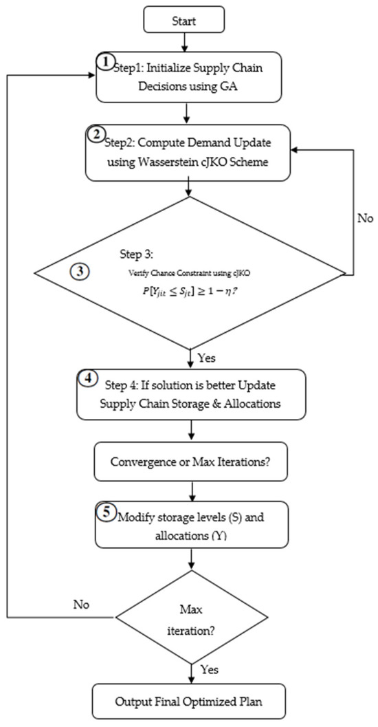
Figure 2.
Iterative metaheuristic optimization framework using cJKO for a distributionally robust supply chain design.
5. Computational Results
5.1. Experimental Setup
The optimization was performed on a machine with an Intel i7-9700 CPU and 16 GB of RAM using Python 3.12 (NumPy, SciPy, DEAP for genetic algorithms, and Matplotlib 3.10.0 for visualization) [41,42,43,44]. The inner optimization problem in the cJKO scheme was solved using COBYLA (Constrained Optimization BY Linear Approximation) from the SciPy library to efficiently handle the Wasserstein-constrained subproblem. The code has been developed in Python and is freely available at the following repository: https://github.com/iman-ie/FacilityLocation_cJKO.git (accessed on 1 May 2025).
To evaluate the performance of the proposed stochastic facility location model under Wasserstein ambiguity and chance constraints, we conduct a comprehensive series of computational experiments using synthetically generated data. The testbed consists of six problem instances with varying scales, including configurations of 15, 30, and 40 customers and candidate facilities, tested over planning horizons of both three and five time periods to assess scalability and temporal complexity handling. The parameter settings follow data generation strategies adapted from well-established studies in the literature on robust and stochastic logistics [19,45]. The synthetic data are generated to simulate a wide range of realistic operating environments with uncertainty in demand and cost. Parameter values are drawn from uniform distributions to ensure heterogeneity across instances. Furthermore, the model is tested under varying values of the Wasserstein radius , allowing a detailed sensitivity analysis on the trade-off between robustness and conservatism. The experimental parameters are detailed in Table 3.
Table 3.
Experimental setup parameters.
5.2. Parameter Setting
The effectiveness of metaheuristic algorithms is significantly impacted by their parameter settings. Consequently, this section focuses on optimizing the parameters of the GA to enhance the robustness of the solution strategy. While traditional studies have often used a full factorial design for parameter selection, this method becomes less practical as the number of parameters increases. To address this issue, the Taguchi method is adopted to streamline the experimental process by reducing the number of required tests and overall complexity [46]. Initially, the test problem is executed ten times. The outcomes of the objective functions are then converted into relative percentage deviation (RPD) values to standardize performance comparison. The average RPD is subsequently utilized to compute signal-to-noise (S/N) ratios, which help identify the most effective parameter levels. Table 4 outlines the selected parameters and their respective levels.
Table 4.
The parameters level of GA.
Based on the defined parameters and their corresponding levels, the L18 orthogonal array from the Taguchi method is applied to the GA. To assess the outcomes of each experimental run, the RPD is calculated using Equation (23):
In this context, denotes the lowest observed value of the cost function, while represents the solution produced by the algorithm [47,48]. Table 5 presents the L18 orthogonal array used in the experiments, along with the average RPD calculated over ten independent runs.
Table 5.
The orthogonal array L18 for the GA.
Taguchi’s method aims to enhance the influences of controllable factors while reducing the effects of noise variables. The ratio serves as a key metric to achieve both objectives. This approach is categorized into three types: “larger is better”, “smaller is better”, and “nominal is best”. In the current study, the RPD is employed as the response variable. Therefore, the “smaller is better” criterion is selected for parameter tuning, and Equation (23) is used to compute the corresponding ratio.
In this context, Y represents the response value for each test instance, and n denotes the total number of experiments based on the orthogonal array. The analysis of the response (RPD) was conducted using Minitab 21.1.0 software. Figure 3 illustrates the average ratios corresponding to each parameter level. Based on the results, the optimal levels for the GA parameters are identified as three, two, one, three, one, and two. Table 6 summarizes the best values for each parameter.
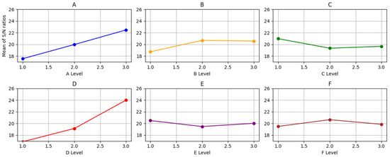
Figure 3.
The GA factors’ mean SN ratio plot: each chart refers to a specific parameter in Table 5.
Table 6.
Optimal GA parameter settings based on the Taguchi S/N ratio analysis.
5.3. Sensitivity Analysis of the Wasserstein Ambiguity Radius
To evaluate the sensitivity of the proposed distributionally robust facility location model with respect to the Wasserstein ambiguity radius , we solve the problem under a range of values. Specifically, we considered . Each instance is solved using the cJKO-based optimization framework, and the corresponding total expected cost (objective value) is computed by aggregating facility setup costs, inventory holding costs, and allocation-based penalties under the resulting worst-case demand distribution. The results relative to the smallest test case (i.e., I = 15, J = 15, and T = 3), which are summarized in Table 7 and illustrated in Figure 4, reveal a non-monotonic trend in the objective value as a function of . Initially, increasing the radius leads to a reduction in the objective, indicating improved robustness to distributional shifts without overcompensating in the decision variables. However, beyond a critical value of , the objective begins to increase, suggesting excessive conservatism as the ambiguity set becomes too large. Figure 5 compares the prescribed Wasserstein radius (ε) with the actual Wasserstein distance achieved after optimization. The observed near-monotonic trend highlights how increasing ε allows the model to explore a broader set of distributions, thereby enabling more robust—but potentially more conservative—solutions. This behavior confirms that the optimization process effectively leverages the flexibility provided by the ambiguity set while maintaining alignment with the WDRO framework.
Table 7.
Costs for different values of the cJKO parameter for the case I = 15, J = 15, and T = 3.
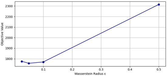
Figure 4.
Effect of the Wasserstein ambiguity radius on the objective value (for the case I = 15, J = 15, and T = 3).
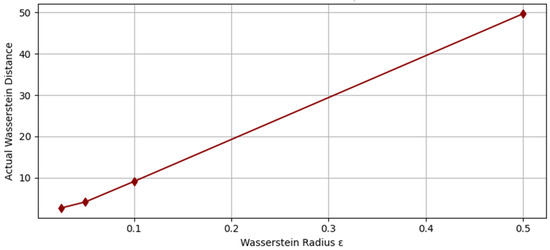
Figure 5.
Actual Wasserstein distance achieved vs. specified radius ε (for the case I = 15, J = 15, and T = 3).
Figure 6 further details the behaviors of both the first-stage cost (on the left) and the overall cost (on the right) with respect to the value of and for 10 independent runs. Obviously, most of the total cost is given by the second-stage cost rather than the first-stage cost. While the first-stage cost monotonically increases with , the overall cost increases non-monotonically. Finally, the variability of the total costs significantly increases with increasing from 0.1 to 0.5 due to the fact that the demand scenarios generated are significantly different from the historical data.
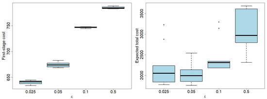
Figure 6.
Effects of the Wasserstein ambiguity radius on the first-stage cost (on the left) and the overall cost (on the right) for the smallest test case (i.e., I = 15, J = 15, and T = 3). Box plots were obtained over 10 independent runs.
The same behavior is also observed for the largest test case, that is, I = 40, J = 40, and T = 5, as reported in Table 8.
Table 8.
Costs for different values of the cJKO parameter for the case I = 40, J = 40, and T = 5.
The observed behavior can be attributed to the interplay between robustness and conservatism inherent in WDRO. For small values of , the model remains vulnerable to a misestimation of demand, while at large values of , the solution tends to over-allocate resources to hedge against highly pessimistic demand realizations. This trade-off directly affects both cost efficiency and feasibility under chance constraints, as a larger generally improves satisfaction probability at the expense of increased operational cost.
Figure 7 illustrates the interplay between the out-of-sample objective value and the empirical satisfaction probability as a function of the Wasserstein radius , which governs the size of the ambiguity set in the distributionally robust optimization model. As shown, the objective value (blue line, left axis) initially increases with , reflecting the model’s increasing conservatism in hedging against distributional shifts. Concurrently, the satisfaction probability (orange dashed line, right axis)—defined as the empirical frequency with which the chance constraints are met across test scenarios—monotonically increases with larger values, starting from 91%. This trend confirms the theoretical expectation that larger ambiguity sets provide more robust solutions by better encompassing the true demand distribution. However, the trade-off becomes evident as overly conservative solutions (large ) yield diminishing returns in feasibility gains while incurring significantly higher costs.
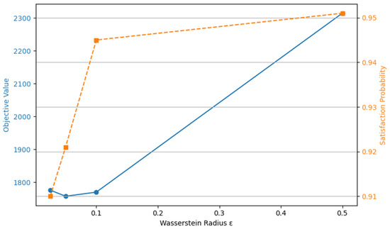
Figure 7.
Effects of on performance and feasibility (for the case I = 15, J = 15, and T = 3).
5.4. Performance Analysis of the Proposed Algorithm
Table 9 demonstrates the superior performance of the proposed cJKO method compared to the Outer Approximation (OA) algorithm from reference [21] and the Robust Optimization (RO) baseline across six problem instances ranging from 15 to 40 facilities and customers over three to five time periods. The cJKO method consistently achieves the lowest objective values across all configurations, outperforming OA by 0.4% to 0.95% and showing even more significant improvements over RO, particularly in instances with longer planning horizons where RO performs poorly (e.g., achieving 6948.55 vs. cJKO’s 5331.98 in the largest instance).
Table 9.
Performance comparison: RO, approach presented in [21] (e.g., OA), and cJKO.
The proposed cJKO approach leverages the Wasserstein distance and transport maps to balance robustness and solution quality more effectively than both benchmark methods, addressing the limitations of OA’s worst-case joint chance constraints and RO’s overly conservative uncertainty hedging. By modeling facility opening decisions as binary matrices over the planning horizon while dynamically managing storage levels under uncertain demand and capacity constraints, the cJKO method demonstrates superior handling of spatial-temporal complexity in facility location and inventory planning problems, maintaining its performance advantages as both the problem size and planning horizons increase.
5.5. Computational Time Analysis
The computational time comparison in Table 10 reveals distinct trade-offs between solution quality and computational efficiency across the three approaches. The RO baseline achieves the fastest execution times (0.46 to 36.87 s), while the OA algorithm exhibits moderate computational requirements (3.33 to 162.73 s). In contrast, the proposed cJKO method requires significantly higher computational resources, with execution times ranging from 224.42 s to 5346.68 s. This computational overhead stems from the iterative nature of the cJKO scheme, which requires solving multiple optimization subproblems at each iteration, computing Wasserstein distances between probability measures, and optimizing transport maps to characterize distributional ambiguity. With this approach, in order to obtain better solution quality through a more accurate uncertainty quantification, the method necessarily incurs substantial computational costs.
Table 10.
Computational time analysis.
The execution time scaling reveals that cJKO is particularly sensitive to increases in planning horizon length, with dramatic time increases when moving from three to five time periods (e.g., from 1561.33 to 5162.91 s for the 30 × 30 configuration). For practical applications, this computational profile makes the cJKO method most suitable for strategic planning scenarios where solution optimality is paramount, while simpler approaches like RO remain preferable for operational decisions requiring rapid response times.
Figure 8 presents the convergence behavior of the optimization algorithm, demonstrating the progressive improvement of the objective function. Initially, the solution explores a wider search space, leading to fluctuations due to the stochastic nature of the optimization process. As the iterations progress, the algorithm stabilizes around a near-optimal solution, reflecting the balance between exploration and exploitation. The sharp decrease in the objective value at a later stage suggests a structural shift in the solution space, possibly due to a critical update in decision variables or constraints. The final stabilization indicates convergence, confirming the algorithm’s ability to efficiently navigate the solution landscape and identify an optimal or near-optimal solution within a finite number of iterations.
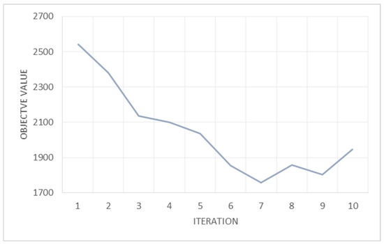
Figure 8.
The convergence behavior of the optimization algorithm.
6. Conclusions
This study introduces an improved chance-constrained optimization framework for facility location under demand uncertainty, integrating a Wasserstein-based distributional approach to enhance robustness. By addressing the inherent variability in demand, the model ensures that probabilistic constraints are satisfied while optimizing facility placement and capacity allocation. Computational experiments across multiple problem instances demonstrate that the proposed cJKO approach consistently outperforms established benchmarks, achieving objective values 0.4% to 0.95% better than the Outer Approximation method and significantly superior results compared to traditional Robust Optimization, particularly in scenarios with extended planning horizons. Furthermore, the incorporation of Wasserstein distance constraints improves robustness against distributional shifts, ensuring that the model remains valid under different demand realizations. This highlights the significance of distributionally robust optimization in facility location problems, enabling more resilient decision-making under uncertainty.
Despite these advantages, some limitations remain. The model assumes to have historical data of demand. Additionally, the computational burden increases substantially with the problem size and planning horizon length, with execution times ranging from minutes to hours for larger instances, necessitating a consideration of the trade-off between solution quality and computational efficiency. The cJKO method’s iterative nature and complex Wasserstein distance computations make it most suitable for strategic planning scenarios where solution optimality justifies the computational investment, while simpler approaches may be preferred for operational decisions requiring a rapid response. Future research could explore adaptive uncertainty sets to refine demand estimates dynamically or integrate real-time learning mechanisms to enhance responsiveness. Extending the framework to multi-stage decision processes or multi-echelon networks would further improve its applicability in complex supply chain systems.
Author Contributions
Conceptualization, F.A. and E.M.; methodology, A.C.; software, I.S.; validation, I.S. and A.C.; writing—original draft preparation, I.S. and F.A.; writing—review and editing, all.; visualization, I.S.; supervision, A.C.; funding acquisition, E.M. All authors have read and agreed to the published version of the manuscript.
Funding
This research was co-funded by the National Research project ULTRA OPTYMAL (Urban Logistics and Sustainable Transportation: Optimization Under Uncertainty and Machine Learning) under the PRIN 2020 program, Italian Ministry for University and Research.
Data Availability Statement
The entire code, including the data generation, is freely available at the following repository: https://github.com/iman-ie/FacilityLocation_cJKO.git (accessed on 1 May 2025).
Conflicts of Interest
The authors declare no conflicts of interest.
References
- Meira, S. Everything Platforms. SSRN. 2025. Available online: https://ssrn.com/abstract=5160171 (accessed on 1 May 2025).
- Xiao, H.; Zhang, J.; Zhang, Z.; Li, W. A Survey of Approximation Algorithms for the Universal Facility Location Problem. Mathematics 2025, 13, 1023. [Google Scholar] [CrossRef]
- Peyré, G.; Cuturi, M. Computational Optimal Transport; CREST Working Papers; CREST: Fort Worth, TX, USA, 2017; pp. 2017–2086. [Google Scholar]
- Peyré, G.; Cuturi, M. Computational optimal transport: With applications to data science. Found. Trends Mach. Learn. 2019, 11, 355–607. [Google Scholar] [CrossRef]
- Uscidda, T.; Cuturi, M. The Monge Gap: A Regularizer to Learn All Transport Maps. In Proceedings of the International Conference on Machine Learning, Hawaii, HI, USA, 23–29 July 2023; PMLR 202, pp. 34709–34733. [Google Scholar]
- Candelieri, A.; Ponti, A.; Archetti, F. Wasserstein enabled Bayesian optimization of composite functions. J. Ambient Intell. Humaniz. Comput. 2023, 14, 11263–11271. [Google Scholar] [CrossRef]
- Jordan, R.; Kinderlehrer, D.; Otto, F. The variational formulation of the Fokker-Planck equation. SIAM J. Math. Anal. 1998, 29, 1–17. [Google Scholar] [CrossRef]
- Xu, S.; Govindan, K.; Wang, W.; Yang, W. Supply chain management under cap-and-trade regulation: A literature review and research opportunities. Int. J. Prod. Econ. 2024, 271, 109199. [Google Scholar] [CrossRef]
- Peidro, D.; Martin, X.A.; Panadero, J.; Juan, A.A. Solving the uncapacitated facility location problem under uncertainty: A hybrid tabu search with path-relinking simheuristic approach. Appl. Intell. 2024, 54, 5617–5638. [Google Scholar] [CrossRef]
- Snyder, L.V. Facility location under uncertainty: A review. IIE Trans. 2006, 38, 547–564. [Google Scholar] [CrossRef]
- Laporte, G.; Nickel, S.; Saldanha-da-Gama, F. Introduction to Location Science; Springer International Publishing: Cham, Switzerland, 2019; pp. 1–21. [Google Scholar]
- Kouvelis, P.; Yu, G. Robust Discrete Optimization and Its Applications; Springer Science & Business Media: Boston, MA, USA, 1996; Volume 14. [Google Scholar]
- Jabbarzadeh, A.; Fahimnia, B.; Seuring, S. Dynamic supply chain network design for the supply of blood in disasters: A robust model with real world application. Transp. Res. Part E Logist. Transp. Rev. 2014, 70, 225–244. [Google Scholar] [CrossRef]
- Shapiro, A.; Dentcheva, D.; Ruszczynski, A. Lectures on Stochastic Programming: Modeling and Theory, 3rd ed.; Shapiro, A., Dentcheva, D., Ruszczynski, A., Eds.; SIAM Publications Library: Philadelphia, PA, USA, 2021. [Google Scholar]
- Ho, C.P.; Petrik, M.; Wiesemann, W. Robust ϕ-Divergence MDPs. Adv. Neural Inf. Process. Syst. 2022, 35, 32680–32693. [Google Scholar]
- Delage, E.; Ye, Y. Distributionally robust optimization under moment uncertainty with application to data-driven problems. Oper. Res. 2010, 58, 595–612. [Google Scholar] [CrossRef]
- Kirschner, J.; Bogunovic, I.; Jegelka, S.; Krause, A. Distributionally Robust Bayesian Optimization. In Proceedings of the International Conference on Artificial Intelligence and Statistics (AISTATS), Online, 26–28 June 2020; PMLR 108, pp. 2174–2184. [Google Scholar]
- Micheli, F.; Balta, E.C.; Tsiamis, A.; Lygeros, J. Wasserstein Distributionally Robust Bayesian Optimization with Continuous Context. arXiv 2025, arXiv:2503.20341. [Google Scholar]
- Liu, K.; Li, Q.; Zhang, Z.H. Distributionally robust optimization of an emergency medical service station location and sizing problem with joint chance constraints. Transp. Res. Part B Methodol. 2019, 119, 79–101. [Google Scholar] [CrossRef]
- Ji, R.; Lejeune, M.A. Data-driven distributionally robust chance-constrained optimization with Wasserstein metric. J. Glob. Optim. 2021, 79, 779–811. [Google Scholar] [CrossRef]
- Wang, Z.; Liu, K.; You, K.; Wang, Z. Wasserstein distributionally robust facility location and capacity planning for disaster relief. Expert Syst. Appl. 2025, 272, 126647. [Google Scholar] [CrossRef]
- Zhang, L.; Yang, J.; Gao, R. A short and general duality proof for Wasserstein distributionally robust optimization. Oper. Res. 2024. [Google Scholar] [CrossRef]
- Bayraksan, G.; Love, D.K. Data-driven stochastic programming using phi-divergences. Oper. Res. Revolut. 2015, 1–19. [Google Scholar] [CrossRef]
- Mohajerin Esfahani, P.; Kuhn, D. Data-driven distributionally robust optimization using the Wasserstein metric: Performance guarantees and tractable reformulations. Math. Program. 2018, 171, 115–166. [Google Scholar] [CrossRef]
- Wang, Z.; Jiang, S.; Lin, Y.; Tao, Y.; Chen, C. A review of algorithms for distributionally robust optimization using statistical distances. J. Ind. Manag. Optim. 2025, 21, 1749–1770. [Google Scholar] [CrossRef]
- Zhou, C.; Bayraksan, G. Effective Scenarios in Distributionally Robust Optimization with Wasserstein Distance. Optimization Online. Available online: https://optimization-online.org/wp-content/uploads/2024/12/Effective_Scen_s_in_DRO_W_paper.pdf (accessed on 20 June 2025).
- Gen, M.; Cheng, R. Genetic Algorithms and Engineering Optimization; John Wiley & Sons: Hoboken, NJ, USA, 1999. [Google Scholar]
- Saeedi, M.; Parhazeh, S.; Tavakkoli-Moghaddam, R.; Khalili-Fard, A. Designing a two-stage model for a sustainable closed-loop electric vehicle battery supply chain network: A scenario-based stochastic programming approach. Comput. Ind. Eng. 2024, 190, 110036. [Google Scholar] [CrossRef]
- Lee, W.; Wang, L.; Li, W. Deep JKO: Time-implicit particle methods for general nonlinear gradient flows. J. Comput. Phys. 2024, 514, 113187. [Google Scholar] [CrossRef]
- Candelieri, A.; Ponti, A.; Archetti, F. A Constrained-JKO Scheme for Effective and Efficient Wasserstein Gradient Flows. In Proceedings of the International Conference on Learning and Intelligent Optimization, Ischia Island, Italy, 9–13 June 2024; Springer Nature: Cham, Switzerland, 2024; pp. 66–80. [Google Scholar]
- Korotin, A.; Egiazarian, V.; Asadulaev, A.; Safin, A.; Burnaev, E. Wasserstein-2 generative networks. arXiv 2019, arXiv:1909.13082. [Google Scholar]
- Korotin, A.; Li, L.; Solomon, J.; Burnaev, E. Continuous Wasserstein-2 barycenter estimation without minimax optimization. In Proceedings of the International Conference on Learning Representations, Vienna, Austria, 4 May 2021. [Google Scholar]
- Mokrov, P.; Korotin, A.; Li, L.; Genevay, A.; Solomon, J.M.; Burnaev, E. Large-scale Wasserstein gradient flows. Adv. Neural Inf. Process. Syst. 2021, 34, 15243–15256. [Google Scholar]
- Korotin, A.; Selikhanovych, D.; Burnaev, E. Kernel neural optimal transport. arXiv 2022, arXiv:2205.15269. [Google Scholar]
- Korotin, A.; Selikhanovych, D.; Burnaev, E. Neural optimal transport. arXiv 2022, arXiv:2201.12220. [Google Scholar]
- Fan, J.; Zhang, Q.; Taghvaei, A.; Chen, Y. Variational Wasserstein gradient flow. Proc. Int. Conf. Mach. Learn. 2022, PMLR 162, 6185–6215. [Google Scholar]
- Candelieri, A.; Ponti, A.; Archetti, F. Generative models via optimal transport and Gaussian processes. In Learning and Intelligent Optimization; Sellmann, M., Tierney, K., Eds.; Springer: Berlin/Heidelberg, Germany, 2023; pp. 135–149. [Google Scholar]
- Kong, Z.; Chaudhuri, K. The expressive power of a class of normalizing flow models. Proc. Int. Conf. Artif. Intell. Stat. 2020, PMLR 108, 3599–3609. [Google Scholar]
- Li, L.; Hurault, S.; Solomon, J.M. Self-consistent velocity matching of probability flows. Adv. Neural Inf. Process. Syst. 2023, 36, 57038–57057. [Google Scholar]
- Holland, J.H. Genetic Algorithms. Sci. Am. 1992, 267, 66–73. [Google Scholar] [CrossRef]
- Harris, C.R.; Millman, K.J.; van der Walt, S.J.; Gommers, R.; Virtanen, P.; Counrnapeau, D.; Wieser, E.; Taylor, J.; Berg, S.; Smith, N.J.; et al. Array programming with NumPy. Nature 2020, 585, 357–362. [Google Scholar] [CrossRef]
- Virtanen, P.; Gommers, R.; Oliphant, T.E.; Haberland, M.; Reddy, T.; Cournapeau, D.; Burovski, E.; Peterson, P.; Weckesser, W.; Bright, J.; et al. SciPy 1.0: Fundamental Algorithms for Scientific Computing in Python. Nat. Methods 2020, 17, 261–272. [Google Scholar] [CrossRef]
- Fortin, F.-A.; Rainville, F.-M.; Gardner, M.-A.; Parizeau, M.; Gagné, C. DEAP: Evolutionary Algorithms Made Easy. J. Mach. Learn. Res. 2012, 13, 2171–2175. [Google Scholar]
- Hunter, J.D. Matplotlib: A 2D Graphics Environment. Comput. Sci. Eng. 2007, 9, 90–95. [Google Scholar] [CrossRef]
- Zhang, Z.H.; Li, K. A novel probabilistic formulation for locating and sizing emergency medical service stations. Ann. Oper. Res. 2015, 229, 813–835. [Google Scholar] [CrossRef]
- Taguchi, G. Introduction to Quality Engineering: Designing Quality into Products and Processes; Asian Productivity Organization: Tokyo, Japan, 1986. [Google Scholar]
- Hosseini Baboli, S.A.; Arabkoohsar, A.; Seyedi, I. Numerical modeling and optimization of pressure drop and heat transfer rate in a polymer fuel cell parallel cooling channel. J. Braz. Soc. Mech. Sci. Eng. 2023, 45, 201. [Google Scholar] [CrossRef]
- Rajabi-Kafshgar, A.; Seyedi, I.; Tirkolaee, E.B. Circular Closed-Loop Supply Chain Network Design Considering 3D Printing and PET Bottle Waste. Environ. Dev. Sustain. 2024, 1–37. [Google Scholar] [CrossRef]


Disclaimer/Publisher’s Note: The statements, opinions and data contained in all publications are solely those of the individual author(s) and contributor(s) and not of MDPI and/or the editor(s). MDPI and/or the editor(s) disclaim responsibility for any injury to people or property resulting from any ideas, methods, instructions or products referred to in the content. |
© 2025 by the authors. Licensee MDPI, Basel, Switzerland. This article is an open access article distributed under the terms and conditions of the Creative Commons Attribution (CC BY) license (https://creativecommons.org/licenses/by/4.0/).