Pseudo-Multiview Learning Using Subjective Logic for Enhanced Classification Accuracy

Abstract

Deep learning has significantly advanced image classification by leveraging hierarchical feature representations. A key factor in enhancing classification accuracy is feature concatenation, which integrates diverse feature sets to provide a richer representation of input data. However, this fusion strategy has inherent limitations, including increased computational complexity, susceptibility to redundant or irrelevant features, and challenges in optimally weighting different feature contributions. To address these challenges, this paper presents a pseudo-multiview learning method that dynamically combines different views at the evidence level using a belief-based model known as subjective logic. This approach adaptively assigns confidence levels to each view, ensuring more effective integration of complementary information while mitigating the impact of noisy or less relevant features. Experimental evaluations of datasets from various domains demonstrate that the proposed method enhances classification accuracy and robustness compared with conventional classification techniques.

1. Introduction

Image classification is a fundamental task in computer vision that involves assigning a label to an image based on its visual content. Traditional methods rely on handcrafted feature extraction techniques such as scale-invariant feature transform (SIFT) [1], histogram of oriented gradients (HOG) [2], and color histograms, followed by a classifier such as support vector machines (SVM) [3] or k-nearest neighbors (k-NN) [4]. While these approaches are effective for specific tasks, they often struggle with complex patterns and require domain expertise for feature engineering.

With the rise of deep learning, convolutional neural networks (CNNs) [5] have revolutionized image classification by automatically learning hierarchical features from raw pixel data. Architectures such as AlexNet [6], VGG [7], ResNet [8], and EfficientNet [9] have achieved state-of-the-art performance on benchmark datasets such as ImageNet [10]. In practice, image classification is widely used in various fields, including medical imaging (e.g., diagnosing diseases from X-ray or MRI scans), autonomous driving (e.g., recognizing pedestrians and traffic signs), and security surveillance (e.g., facial recognition for authentication). The shift from traditional techniques to deep learning has significantly improved accuracy and robustness, making image classification a cornerstone of modern artificial intelligence (AI) applications.

Feature combination plays an important role in enhancing classification accuracy by integrating diverse information sources to provide a more comprehensive representation of data. Among various fusion strategies, feature concatenation [11] is widely used due to its simplicity and effectiveness in combining multiple feature sets, allowing deep learning models to leverage complementary information. However, this approach often increases the model’s capacity, leading to the confidence calibration problem (CCP) [12], where the model becomes overconfident in its predictions, reducing reliability. Addressing CCP requires incorporating uncertainty into the classification process. Uncertainty-aware classifiers, including Bayesian-based [13,14] and non-Bayesian-based methods [15,16], have been explored to mitigate this issue. However, Bayesian-based methods are computationally expensive, making them impractical for real-time applications, while non-Bayesian-based methods are typically limited to single-view data, restricting their generalizability.

Traditional neural network classifiers with softmax layers produce outputs that lie on a probability simplex, representing class probabilities. However, these outputs are often misinterpreted as confidence scores despite lacking explicit representation of uncertainty. In contrast, the Dirichlet distribution models a probability density over the simplex, allowing for the representation of second-order probabilities and the associated uncertainty. Subjective logic [17]—an extension of probabilistic logic that incorporates uncertainty and subjectivity—leverages this capability to express not only predictions but also the uncertainty surrounding those predictions.

The proposed method utilizes subjective logic to fuse information from multiple views at the evidence level rather than at the feature or output level, as in conventional approaches. This strategy enhances model reliability and robustness by preserving uncertainty throughout the decision-making process. Specifically, pseudo-multiview data are generated from a single input, with each view modeled using a variational Dirichlet distribution. The parameters of these distributions are estimated from the extracted evidence across views. An averaging fusion rule is then applied to integrate the evidence, resulting in a robust and uncertainty-aware classification framework-validated empirically across diverse datasets.

The main contribution of this paper is a pseudo-multiview classification method that introduces a new paradigm for integrating multiview information in a reliable and uncertainty-aware manner. The remainder of this paper is organized as follows: Section 3 provides preliminary background information, followed by the description of the proposed method in Section 4. Section 5 presents experimental results to validate the superiority of the proposed method, and Section 6 concludes the paper.

2. Uncertainty-Aware Classification

In safety-critical and high-stakes applications, the reliability of neural network predictions is as important as their accuracy. Traditional deterministic models, which output point estimates, often lack the ability to quantify uncertainty, potentially leading to overconfident and erroneous decisions [12]. Uncertainty-aware classification addresses this limitation by equipping models with mechanisms to express confidence in their predictions. This section provides an overview of key developments in uncertainty estimation, particularly focusing on Bayesian neural networks (BNNs), ensemble methods, and recent innovations in lightweight and scalable uncertainty modeling.

Bayesian learning forms the foundation of uncertainty-aware modeling by treating network parameters as probabilistic entities. A comprehensive survey in [18] outlines various algorithmic strategies for BNNs, including variational inference, Markov Chain Monte Carlo (MCMC), and stochastic gradient methods, offering both theoretical insights and practical guidance for scalable Bayesian modeling. Among the most influential approaches is Monte Carlo Dropout (MCDO) [19], which interprets dropout at inference time as approximate Bayesian inference. MCDO enables uncertainty estimation with minimal architectural changes and has served as a cornerstone in lightweight Bayesian approximations.

A recent work [20] is a plug-and-play method for retrofitting pretrained models with Bayesian capabilities using dropout-based techniques and variational inference. This approach democratizes uncertainty estimation by removing the need for training from scratch, making it highly practical in industrial settings.

Ensemble-based methods have also gained significant traction due to their empirical robustness. Deep Ensembles [21] is a simple yet powerful method that aggregates predictions from independently trained models. This approach captures both epistemic and aleatoric uncertainty and has been widely adopted in diverse domains. However, the resource cost of training and storing multiple models prompted further research into more efficient ensemble mechanisms. For example, [22] compared deep ensembles with committee-based models in molecular dynamics, revealing ensemble superiority in terms of uncertainty calibration and active learning efficiency.

To address the trade-off between scalability and uncertainty quality, Deep Combinatorial Aggregation [23] leverages combinatorial sub-networks within a single model to approximate the diversity of ensembles. Similarly, Credal Deep Ensembles [24] introduced a credal framework to explicitly model prediction imprecision using credal sets, further enriching uncertainty representation with a formal decision-theoretic foundation.

Single-model uncertainty estimation has also seen a rapid evolution. The Deterministic Uncertainty Quantification framework [15] introduced a distance-aware Gaussian process-inspired mechanism, allowing a single deterministic network to produce uncertainty-aware outputs. Extending this paradigm, iterative models with feedback loops were adapted for uncertainty estimation in [25], demonstrating that recurrent-style refinement improves both predictive performance and uncertainty calibration.

In domain-shifted environments, uncertainty plays a crucial role in identifying distributional discrepancies. Pseudo-calibration [26] addresses this challenge by integrating unsupervised domain adaptation with confidence-aware calibration techniques. This method aligns predictions from source and target domains while correcting for overconfident misclassifications, yielding better generalization under distribution shift.

Although many of these methods target classification tasks, uncertainty modeling has also been effectively applied in adjacent areas such as video compression. An efficient perceptual video compression framework in [27] leverages deep saliency prediction and just noticeable distortion modeling. While not directly focused on classification, their work incorporates uncertainty-aware principles by adapting compression quality based on predicted perceptual sensitivity, emphasizing the broader relevance of uncertainty estimation across vision tasks.

Together, these approaches illustrate the rich and evolving landscape of uncertainty-aware classification. From Bayesian approximations and ensembles to deterministic and domain-adaptive strategies, each method offers unique trade-offs between complexity, scalability, and uncertainty fidelity. These tools form the methodological backbone for building reliable and interpretable AI systems capable of operating under ambiguity and risk.

3. Preliminaries

3.1. Subjective Logic

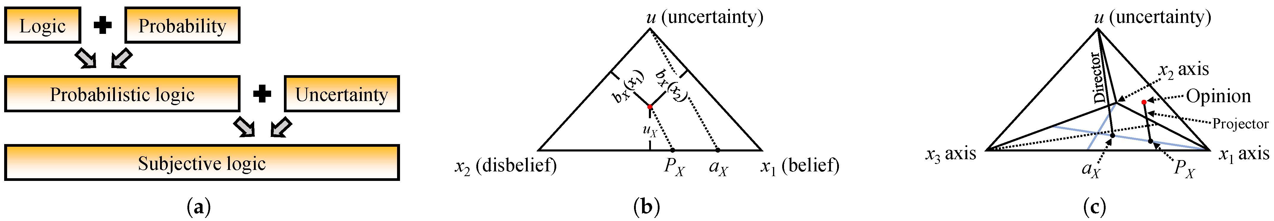
Uncertainty is a fundamental aspect of human reasoning—no statement about the world can be known with absolute certainty, and all assertions are inherently subjective. Subjective logic formalizes this perspective by extending probabilistic logic to explicitly model uncertainty through opinions and structured constructs that encode belief masses, uncertainty, and base rates.

As shown in Figure 1, each opinion represents beliefs over a defined state space and may include the belief source. Belief masses are subadditive, typically summing to less than one, reflecting incomplete information. Mathematically, opinions are equivalent to beta or Dirichlet distributions, with belief masses corresponding to the amount of supporting evidence. With infinite evidence, beliefs become additive; with finite evidence, subadditivity persists—capturing the essence of uncertainty in a principled way.

Let $\mathbb{X}=\{x_1,x_2,\dots ,x_K\}$ be the state space of cardinality K, and let $X\in \mathbb{X}$ be a random variable. The opinion ${\omega }_X$ can then be expressed as follows:

$${\omega }_X=\left({\mathbf{b}}_X,u_X,{\mathbf{a}}_X\right),$$

(1)

where $u_X$ is the uncertainty mass, ${\mathbf{b}}_X$ is the belief mass distribution such that $u_X+{\sum }_i{b}_X\left(x_i\right)=1$, and ${\mathbf{a}}_X$ is the base rate distribution where ${\sum }_i{a}_X\left(x_i\right)=1$. The boldfaced representation indicates that the corresponding variable is a vector. The projected probability $P_X\left(x_i\right)$ is calculated as

$$P_X\left(x_i\right)=b_X\left(x_i\right)+u_X·a_X\left(x_i\right).$$

(2)

In the binary case ($K=2$), a binomial opinion can be visualized within an equilateral triangle (Figure 1b), where each point represents a triplet $(x_1,x_2,u)$ for belief, disbelief, and uncertainty. The triangle’s vertices correspond to full belief, disbelief, and uncertainty, with the base rate ($a_X$) marked on the baseline. The expected probability ($P_X$) is found by projecting the opinion point onto this baseline, parallel to the line connecting the base rate to the triangle’s apex.

Binomial opinions are classified as uncertain (UB) when $u>0$ and dogmatic (DB) when $u=0$, the latter aligning with traditional scalar probabilities.

For $K>2$, opinions are multinomial and harder to visualize. The simplest case, $K=3$, forms a trinomial opinion represented as a point inside a tetrahedron (Figure 1c). The height indicates uncertainty and distances to the side planes correspond to belief masses. The expected probability is obtained by projecting the opinion point onto the base plane parallel to the line from the tetrahedron’s apex to the base rate point.

The general form of a multinomial probability distribution over a state space of cardinality K is captured by the K-dimensional Dirichlet probability density function (PDF). A notable special case arises when the space is binary ($K=2$), in which the distribution simplifies to the well-known Beta density function. For compact notation, let ${\mathbf{p}}_X=\left\{p_X\left(x_i\right)|1\le i\le K\right\}$ denote the vector of probabilities, and ${\mathit{\alpha }}_X=\left\{{\alpha }_X\left(x_i\right)|1\le i\le K\right\}$ the vector of input evidence parameters. The Dirichlet density function over the space $\mathbb{X}$, denoted as $\mathrm{D}\left({\mathbf{p}}_X|{\mathit{\alpha }}_X\right)$, is given by

$$\mathrm{D}\left({\mathbf{p}}_X|{\mathit{\alpha }}_X\right)={\displaystyle \frac{\Gamma \left({\sum }_{i=1}^K{\alpha }_X\left(x_i\right)\right)}{{\prod }_{i=1}^K\Gamma \left({\alpha }_X\left(x_i\right)\right)}}\prod _{i=1}^K{p}_X\left(x_i\right),$$

(3)

where $\Gamma (·)$ is the gamma function, ${\sum }_i{p}_X\left(x_i\right)=1$, and ${\alpha }_X\left(x_i\right)=r_X\left(x_i\right)+W{a}_X\left(x_i\right)$, with $r_X\left(x_i\right)$ representing the number of observations of $x_i$, $a_X\left(x_i\right)$ its base rate, and W the non-informative prior weight.

Over the same space $\mathbb{X}$, the multinomial opinion ${\omega }_X=\left({\mathbf{b}}_X,u_X,{\mathbf{a}}_X\right)$ and the Dirichlet PDF $\mathrm{D}\left({\mathbf{p}}_X|{\mathbf{r}}_X,{\mathbf{a}}_X\right)$ are equivalent through the following mapping:

$$\begin{array}{ccc}\hfill b_X\left(x_i\right)& =& {\displaystyle \frac{r_X\left(x_i\right)}{W+{\sum }_i{r}_X\left(x_i\right)}},\hfill \end{array}$$

(4)

$$\begin{array}{ccc}\hfill u_X& =& {\displaystyle \frac{W}{W+{\sum }_i{r}_X\left(x_i\right)}}.\hfill \end{array}$$

(5)

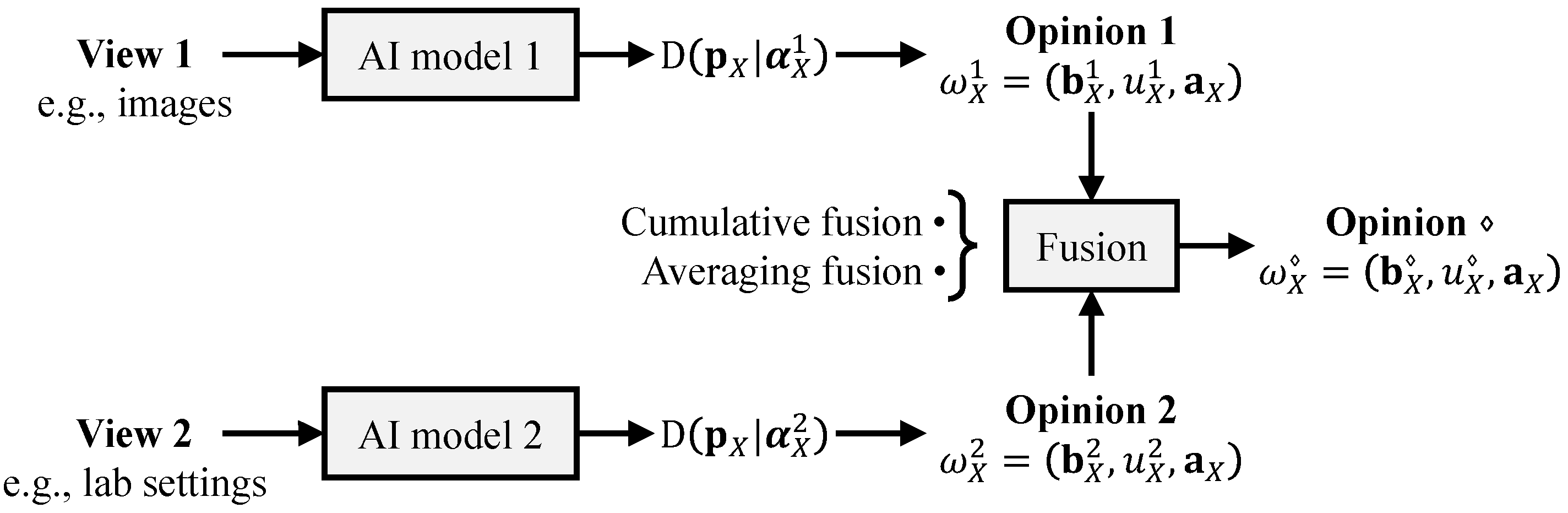
3.2. Opinion Fusion

In many real-world applications, multiple sources contribute distinct sets of evidence, requiring effective fusion techniques to integrate the information. Consider a scenario involving two AI models (illustrated in Figure 2), which results in two different fusion strategies depending on the temporal relationship between their observations:

• Cumulative fusion: When the AI models operate during non-overlapping time intervals, their outputs are considered independent. In this case, the most appropriate approach is to sum up the evidence collected from both models. This additive strategy forms the foundation of cumulative fusion.
• Averaging fusion: When both models operate simultaneously, their outputs are dependent, and a different fusion method is required. In this situation, averaging their outputs is the appropriate strategy, leading to averaging fusion.

Let ${\omega }_X^1=\left({\mathbf{b}}_X^1,u_X^1,{\mathbf{a}}_X\right)$ and ${\omega }_X^2=\left({\mathbf{b}}_X^2,u_X^2,{\mathbf{a}}_X\right)$ be the two opinions, and let $\mathrm{D}\left({\mathbf{p}}_X|{\mathbf{r}}_X^1,{\mathbf{a}}_X\right)$ and $\mathrm{D}\left({\mathbf{p}}_X|{\mathbf{r}}_X^2,{\mathbf{a}}_X\right)$ be their corresponding Dirichlet PDFs. The fused opinions in the two cases are given as follows:

$$\begin{array}{ccc}\hfill {\omega }_X^{\diamond }\left(\mathrm{cumulative}\right)& =& \left({\mathbf{b}}_X^{\diamond },u_X^{\diamond },{\mathbf{a}}_X\right)\sim \mathrm{D}\left({\mathbf{p}}_X|{\alpha }_X^{\diamond }\right)=\mathrm{D}\left({\mathbf{p}}_X|{\mathbf{r}}_X^1+{\mathbf{r}}_X^2,{\alpha }_X\right),\hfill \end{array}$$

(6)

$$\begin{array}{ccc}\hfill {\omega }_X^{\diamond }\left(\mathrm{averaging}\right)& =& \left({\mathbf{b}}_X^{\diamond },u_X^{\diamond },{\mathbf{a}}_X\right)\sim \mathrm{D}\left({\mathbf{p}}_X|{\alpha }_X^{\diamond }\right)=\mathrm{D}\left({\mathbf{p}}_X|{\displaystyle \frac{{\mathbf{r}}_X^1+{\mathbf{r}}_X^2}{2}},{\alpha }_X\right).\hfill \end{array}$$

(7)

4. Proposed Method

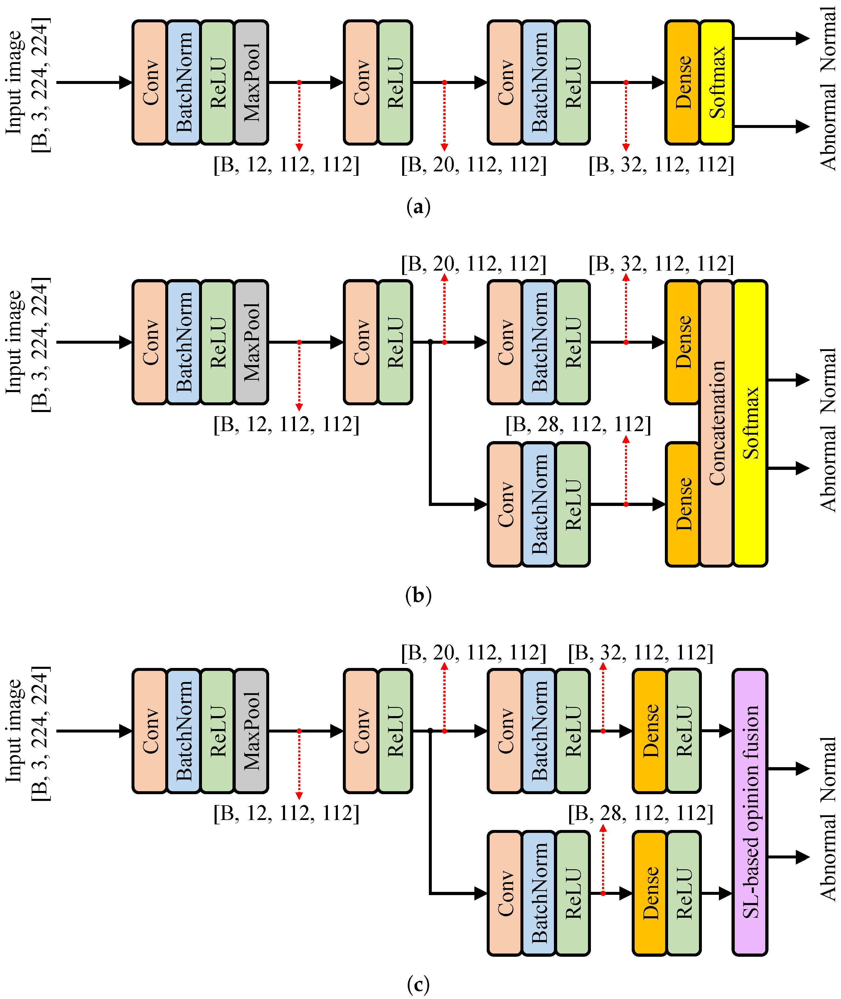
Figure 3 depicts the proposed pseudo-multiview learning model (Figure 3c) alongside two benchmark models: the base model (Figure 3a) and the concatenation model (Figure 3b). The task involves binary classification using RGB input images of size $224\times 224$. A distinct difference of the proposed model is its use of subjective logic instead of the conventional softmax function employed by the benchmark models.

Neural networks are capable of extracting informative evidence from input data, which can then be used to form classification opinions [28]. A conventional neural network classifier can be seamlessly adapted into an evidence-based classifier with minimal modifications. Specifically, in Figure 3c, the typical softmax layer is replaced by ReLU activations to ensure that the network produces non-negative outputs suitable for opinion fusion based on subjective logic. These ReLU outputs are interpreted as an evidence vector ${\mathbf{e}}_X$, from which Dirichlet distribution parameters are computed as ${\mathit{\alpha }}_X={\mathbf{e}}_X+1$. Subsequently, the averaging opinion fusion strategy (depicted in Figure 2) is applied to obtain the final output.

To enable effective training, the standard cross-entropy loss used in image classification is modified to suit the evidence-based framework. The revised loss function, shown in Equation (9), incorporates the digamma function $\psi (·)$, the Dirichlet strength $S={\sum }_{i=1}^K{\mathit{\alpha }}_X\left(x_i\right)$, and the ground truth label $y_i$. This formulation encourages the model to accumulate more evidence for the correct class during training. However, on its own, it does not penalize evidence accumulation for incorrect classes. To mitigate this problem, an additional KL divergence term, shown in Equation (10), is introduced, using the adjusted Dirichlet parameters ${\tilde{\alpha }}_X$, which helps preserve evidence for the correct class while suppressing it for incorrect ones.

Given the Dirichlet parameter ${\mathit{\alpha }}_X\left(x_i\right)$ for each sample of $x_i$, the complete sample-specific loss function is presented in Equation (11), with $\lambda$ serving as a balancing coefficient between the evidence-encouraging and evidence-penalizing components.

To ensure that all views or input perspectives contribute meaningful and consistent opinions, the model employs a multi-task learning strategy. This approach utilizes a combined overall loss function, shown in Equation (11), which promotes collaborative learning across views to improve the quality of the aggregated opinion.

$$\begin{array}{ccc}\hfill {\mathcal{L}}_{\mathrm{mCE}}\left({\mathit{\alpha }}_X\right)& =& \sum _{i=1}^K{y}_i\left(\psi \left(S\right)-\psi \left({\mathit{\alpha }}_X\right)\right),\hfill \end{array}$$

(8)

$$\begin{array}{ccc}\hfill \mathrm{KL}\left(\mathrm{D}\left({\mathbf{p}}_X|{\tilde{\mathit{\alpha }}}_X\right)\left|\right|\mathrm{D}\left({\mathbf{p}}_X|\mathbf{1}\right)\right)& =& \log {\displaystyle \frac{\Gamma \left({\sum }_{i=1}^K{\tilde{\mathit{\alpha }}}_X\left(x_i\right)\right)}{\Gamma \left(K\right){\prod }_{i=1}^K\Gamma \left({\mathit{\alpha }}_X\left(x_i\right)\right)}}\hfill \\ \hfill & & +\sum _{i=1}^K\left({\tilde{\mathit{\alpha }}}_X\left(x_i\right)-1\right)\left(\psi \left({\tilde{\mathit{\alpha }}}_X\left(x_i\right)\right)-\psi \left(\sum _{i=1}^K{\tilde{\mathit{\alpha }}}_X\left(x_i\right)\right)\right),\hfill \end{array}$$

(9)

$$\begin{array}{ccc}\hfill \mathcal{L}\left({\mathit{\alpha }}_X\right)& =& {\mathcal{L}}_{\mathrm{mCE}}\left({\mathit{\alpha }}_X\right)+\lambda ·\mathrm{KL}\left(\mathrm{D}\left({\mathbf{p}}_X|{\tilde{\mathit{\alpha }}}_X\right)\left|\right|\mathrm{D}\left({\mathbf{p}}_X|\mathbf{1}\right)\right),\hfill \end{array}$$

(10)

$$\begin{array}{ccc}\hfill {\mathcal{L}}_{\mathrm{overall}}& =& \sum _{i=1}^K\left(\mathcal{L}\left({\mathit{\alpha }}_X\left(x_i\right)\right)+\sum _{j=1}^N\mathcal{L}\left({\mathit{\alpha }}_X^j\left(x_i\right)\right)\right).\hfill \end{array}$$

(11)

5. Experimental Results

5.1. Experimental Settings

In this section, we evaluate the proposed model using four real-world datasets: BreakHis [29], Oxford-IIIT [30], Chest X-ray [31], and a Plant Leaf Disease dataset [32].

The BreakHis dataset contains 9109 microscopic images of breast tumor tissue collected from 82 patients, captured under four different magnification levels ($40\times$, $100\times$, $200\times$, and $400\times$). It includes 2480 benign and 5429 malignant samples, offering a rich and diverse set for binary classification tasks.

The Oxford-IIIT pet dataset includes 37 categories of cat and dog breeds, with approximately 200 images per class. These images exhibit significant variation in scale, pose, and lighting conditions. Each image is annotated with ground truth breed labels, making the dataset well-suited for fine-grained visual recognition.

The Chest X-ray dataset consists of 5863 radiographic images labeled as either pneumonia or normal. These images were obtained from pediatric patients aged one to five years at Guangzhou Women and Children’s Medical Center. All X-rays were captured as part of routine clinical procedures. To ensure high data quality, low-resolution or unreadable scans were excluded. Diagnoses were validated by two expert radiologists, with a third expert reviewing the evaluation set to minimize labeling errors and improve the reliability of the dataset for training and testing AI models.

Lastly, the Plant Leaf Disease dataset features approximately 87,000 images of crop leaves, representing both healthy samples and those affected by various diseases. The dataset spans 38 distinct classes, enabling robust evaluation of classification in agricultural diagnostics.

All experiments were conducted with three models: the base model, the concatenation model, and the proposed pseudo-multiview learning model. Five-fold cross-validation was employed, and hyperparameter tuning was performed using the Microsoft Neural Network Intelligence toolkit [33]. The learning rate and batch size were searched over the ranges $[{10}^{-4},{10}^{-1}]$ and $\{8,32,64,256,512,1024\}$, respectively. Early stopping was applied, terminating training if no improvement was observed over ten consecutive epochs.

5.2. Comparison with Base and Concatenation Models

The experimental results, summarized in

Table 1. Evaluation of classification performance on different real-world datasets. Best results are boldfaced.

Dataset		Metric	Base	Concatenation	Proposed
BreakHis	$40\times$	AUC	0.566 ± 0.027	$\mathbf{0}.\mathbf{586}\pm \mathbf{0}.\mathbf{056}$	0.584 ± 0.041
	$100\times$		0.571 ± 0.099	0.631 ± 0.055	$\mathbf{0}.\mathbf{648}\pm \mathbf{0}.\mathbf{050}$
	$200\times$		0.597 ± 0.141	0.693 ± 0.014	$\mathbf{0}.\mathbf{694}\pm \mathbf{0}.\mathbf{025}$
	$400\times$		0.641 ± 0.072	0.651 ± 0.050	$\mathbf{0}.\mathbf{677}\pm \mathbf{0}.\mathbf{029}$
Oxford-IIIT			0.651 ± 0.059	0.768 ± 0.091	$\mathbf{0}.\mathbf{808}\pm \mathbf{0}.\mathbf{029}$
Chest X-ray			0.901 ± 0.018	0.898 ± 0.024	$\mathbf{0}.\mathbf{901}\pm \mathbf{0}.\mathbf{014}$
Plant leaf disease			0.781 ± 0.078	$\mathbf{0}.\mathbf{991}\pm \mathbf{0}.\mathbf{005}$	0.988 ± 0.003
BreakHis	$40\times$	ACC	0.570 ± 0.024	0.599 ± 0.049	$\mathbf{0}.\mathbf{613}\pm \mathbf{0}.\mathbf{044}$
	$100\times$		0.560 ± 0.080	0.588 ± 0.034	$\mathbf{0}.\mathbf{623}\pm \mathbf{0}.\mathbf{076}$
	$200\times$		0.477 ± 0.187	0.589 ± 0.018	$\mathbf{0}.\mathbf{657}\pm \mathbf{0}.\mathbf{045}$
	$400\times$		0.558 ± 0.131	0.581 ± 0.038	$\mathbf{0}.\mathbf{621}\pm \mathbf{0}.\mathbf{035}$
Oxford-IIIT			0.608 ± 0.040	0.712 ± 0.054	$\mathbf{0}.\mathbf{725}\pm \mathbf{0}.\mathbf{033}$
Chest X-ray			0.809 ± 0.016	0.834 ± 0.015	$\mathbf{0}.\mathbf{861}\pm \mathbf{0}.\mathbf{013}$
Plant leaf disease			0.699 ± 0.162	0.959 ± 0.011	$\mathbf{0}.\mathbf{962}\pm \mathbf{0}.\mathbf{004}$

, clearly demonstrate the effectiveness of the proposed pseudo-multiview learning method based on subjective logic. The evaluation spans four real-world datasets across diverse domains, using both AUC and accuracy as performance metrics. The proposed method demonstrates consistent improvement over both the base and concatenation baselines, particularly in complex or ambiguous classification scenarios.

5.2.1. BreakHis Dataset ($40\times$ to $400\times$ Magnifications)

The proposed method consistently outperforms the base and concatenation approaches across all magnifications in terms of AUC. The performance gap becomes more pronounced at higher magnifications. For example, compared with the base model, the gap increases from $0.018$ at $40\times$ to $0.036$ at $400\times$. This improvement highlights the robustness of the proposed method to finer-grained visual variations.

Similarly, significant improvements are observed in accuracy. For example, at $200\times$ magnification, the proposed method achieves $0.657$ accuracy, a substantial improvement over the base ($0.477$) and concatenation ($0.589$), indicating a strong ability to handle noisy and heterogeneous data.

5.2.2. Oxford-IIIT Dataset

The proposed method achieves an AUC of $0.808$ and an accuracy of $0.725$, corresponding to improvements of $0.157$ ($24.1\%$) and $0.117$ ($19.2\%$), respectively, over the base model. Compared with the concatenation approach, the improvements are $0.04$ ($5.2\%$) in AUC and $0.013$ ($1.8\%$) in accuracy. This dataset, which includes substantial intra-class variation and cluttered backgrounds, benefits notably from the proposed uncertainty-aware fusion strategy.

5.2.3. Chest X-Ray Dataset

Although all methods perform well in AUC, with values around $0.9$, the observed improvements in accuracy—$0.052$ ($6.4\%$) and $0.027$ ($3.2\%$) compared with base and concatenation approaches, respectively—suggest that the proposed method makes more accurate and confident predictions. This gain may be attributed to its enhanced ability to handle ambiguous and borderline cases.

5.2.4. Plant Leaf Disease Dataset

This domain exhibits the most dramatic improvement. The AUC rises from $0.781$ (base) to $0.988$ (proposed), and the accuracy rises from $0.699$ to $0.962$. The gains are especially notable, indicating the strength of the proposed method in leveraging subtle multiview features when uncertainty is high (for example, due to visual similarity between disease symptoms).

The concatenation approach, while improving over the base model in many cases, fails to fully exploit the complementary nature of multiview features, likely due to its simplistic feature-level fusion. It does not model uncertainty and hence may produce overconfident or unreliable predictions, especially under distribution shifts or ambiguous shifts.

In contrast, the proposed method integrates subjective logic to model belief, disbelief, and uncertainty masses derived from individual views. This characteristic not only results in higher predictive performance but also reflects greater model calibration and robustness. Furthermore, the most significant improvements are observed in datasets with complex visual characteristics, underscoring the practical utility of the proposed method in real-world applications that involve noisy, heterogeneous, or multiscale data.

5.3. Comparison with Uncertainty-Aware Methods

In this section, we compare the proposed method with uncertainty-aware models, including Monte-Carlo Dropout (MCDO) [19], Uncertainty-aware Attention (UA) [34], and Evidential Deep Learning (EDL) [35]. MDCO treats dropout at inference time as a Bayesian approximation, enabling the estimation of predictive uncertainty through multiple stochastic forward passes. UA extends this idea by incorporating uncertainty directly into the attention mechanism, allowing models to focus on more reliable features while providing interpretable insights. EDL further advances uncertainty quantification by modeling predictions as evidence distributions over class probabilities, enabling the network to output both belief and uncertainty without requiring sampling. These methods form the foundation for robust and trustworthy AI systems, particularly in high-stakes applications.

All three uncertainty-aware methods—MCDO, UA, and EDL—operate on single-view data and are implemented based on the base model illustrated in Figure 3a. MCDO introduces no additional parameters, while UA and EDL slightly increase the parameter count due to the use of attention modules and minor changes to the output layer, respectively.

Table 2. Evaluation of classification performance on different real-world datasets using uncertainty-aware methods. Best results are boldfaced.

Dataset		Metric	MCDO	UA	EDL	Proposed
BreakHis	$40\times$	AUC	0.561 ± 0.035	0.576 ± 0.031	0.579 ± 0.029	$\mathbf{0}.\mathbf{584}\pm \mathbf{0}.\mathbf{041}$
	$100\times$		0.600 ± 0.032	0.622 ± 0.030	0.633 ± 0.028	$\mathbf{0}.\mathbf{648}\pm \mathbf{0}.\mathbf{050}$
	$200\times$		0.665 ± 0.025	0.681 ± 0.021	0.688 ± 0.020	$\mathbf{0}.\mathbf{694}\pm \mathbf{0}.\mathbf{025}$
	$400\times$		0.638 ± 0.031	0.659 ± 0.029	0.670 ± 0.027	$\mathbf{0}.\mathbf{677}\pm \mathbf{0}.\mathbf{029}$
Oxford-IIIT			0.772 ± 0.033	0.791 ± 0.027	0.798 ± 0.025	$\mathbf{0}.\mathbf{808}\pm \mathbf{0}.\mathbf{029}$
Chest X-ray			0.876 ± 0.015	0.889 ± 0.012	0.897 ± 0.012	$\mathbf{0}.\mathbf{901}\pm \mathbf{0}.\mathbf{014}$
Plant leaf disease			0.961 ± 0.014	0.973 ± 0.011	0.981 ± 0.009	$\mathbf{0}.\mathbf{988}\pm \mathbf{0}.\mathbf{003}$
BreakHis	$40\times$	ACC	0.578 ± 0.030	0.596 ± 0.026	0.607 ± 0.024	$\mathbf{0}.\mathbf{613}\pm \mathbf{0}.\mathbf{044}$
	$100\times$		0.590 ± 0.027	0.608 ± 0.025	0.617 ± 0.026	$\mathbf{0}.\mathbf{623}\pm \mathbf{0}.\mathbf{076}$
	$200\times$		0.617 ± 0.022	0.635 ± 0.019	0.647 ± 0.018	$\mathbf{0}.\mathbf{657}\pm \mathbf{0}.\mathbf{045}$
	$400\times$		0.586 ± 0.034	0.603 ± 0.030	0.615 ± 0.028	$\mathbf{0}.\mathbf{621}\pm \mathbf{0}.\mathbf{035}$
Oxford-IIIT			0.681 ± 0.028	0.704 ± 0.023	0.712 ± 0.021	$\mathbf{0}.\mathbf{725}\pm \mathbf{0}.\mathbf{033}$
Chest X-ray			0.825 ± 0.016	0.842 ± 0.015	0.853 ± 0.014	$\mathbf{0}.\mathbf{861}\pm \mathbf{0}.\mathbf{013}$
Plant leaf disease			0.931 ± 0.013	0.944 ± 0.010	0.952 ± 0.008	$\mathbf{0}.\mathbf{962}\pm \mathbf{0}.\mathbf{004}$

presents a comparative evaluation of the proposed method against these approaches.

5.3.1. BreakHis Dataset ($40\times$ to $400\times$ Magnifications)

The proposed method consistently outperforms MCDO, UA, and EDL at all magnification levels. The performance margin becomes more pronounced at higher magnifications. For example, at $400\times$, the proposed method achieves an AUC of $0.677$, compared with $0.670$ (EDL), $0.659$ (UA), and $0.638$ (MCDO). In terms of accuracy, the proposed method also shows the highest score across all magnifications. Notably, at $200\times$, it achieves $0.657$, significantly surpassing EDL ($0.647$), UA ($0.635$), and MCDO ($0.617$).

The consistent superiority of the proposed method across all scales demonstrates its robustness to high-resolution and complex visual features, where uncertainty modeling plays a crucial role.

5.3.2. Oxford-IIIT Dataset

The proposed method achieves the highest AUC of $0.808$, slightly outperforming ELD ($0.798$) and UA ($0.791$). Similarly, it attains the best accuracy of $0.725$, making a notable improvement over MCDO ($0.681$). Given the high intra-class variation in this dataset, the results suggest that the proposed method offers improved discriminative power and more reliable predictions.

5.3.3. Chest X-Ray Dataset

All methods perform relatively well on this dataset, with marginal differences in AUC. The proposed method achieves an AUC of $0.901$, which is comparable to EDL ($0.879$) and slightly higher than UA ($0.889$) and MCDO ($0.876$). A similar trend for accuracy is observed, where the proposed method achieves $0.861$, demonstrating its ability to handle subtle diagnostic features more reliably.

5.3.4. Plant Leaf Disease Dataset

Although all methods perform well on this low-uncertainty dataset, the proposed model achieves the highest scores in both AUC and accuracy. This result highlights that the proposed method remains beneficial even in domains with low uncertainty, reinforcing its strong generalization capability.

Overall, MCDO offers a simple yet effective approximation of Bayesian inference, but its performance lags behind due to its limited expressiveness and reliance on sampling. UA improves attention by considering uncertainty but still lacks full probabilistic modeling. EDL delivers stronger uncertainty modeling through evidential theory, often ranking second and comparable results. The proposed method, by explicitly modeling belief, disbelief, and uncertainty through subjective logic, achieves more reliable and calibrated predictions. Its consistent dominance in both AUC and accuracy across datasets underscores its effectiveness.

5.4. Model Size Evaluation

The parameter count comparison in

Table 3. Parameter counts of different models.

Model	Parameter Count
Base	409,718
Concatenation	1,518,658
MCDO	409,718
UA	430,204
EDL	413,816
Proposed	766,020

provides important insight into the trade-off between model complexity and performance. The base model has the smallest footprint, with $409,718$ parameters, shared also by MCDO, which does not introduce additional parameters as it only modifies inference behavior using dropout. UA and EDL, on the other hand, slightly increase the parameter count to $430,204$ and $413,816$, respectively, due to the inclusion of attention mechanisms and evidential output layers.

The concatenation model shows a substantial jump in complexity, reaching $1,518,658$ parameters—nearly $3.7\times$ the size of the base model—because it stacks multiple feature extractors without fusion optimization. Despite this increase, it does not consistently outperform lighter uncertainty-aware models, indicating inefficiency in its parameter usage.

The proposed method, with $766,020$ parameters, strikes a balance between model complexity and performance. Although it is not the smallest model, it remains significantly more efficient than the concatenation model, using only about $50\%$ of its parameters. Importantly, the proposed method consistently delivers the best performance across various real-world datasets in terms of both AUC and accuracy. This highlights the effectiveness of its uncertainty modeling strategy, which leverages subjective logic to fuse evidence from multiple sources in a parameter-efficient manner.

In summary, the proposed method offers a compelling trade-off: it avoids the redundancy of the concatenation model while outperforming all other methods—including those with fewer parameters—by intelligently incorporating uncertainty into the learning process.

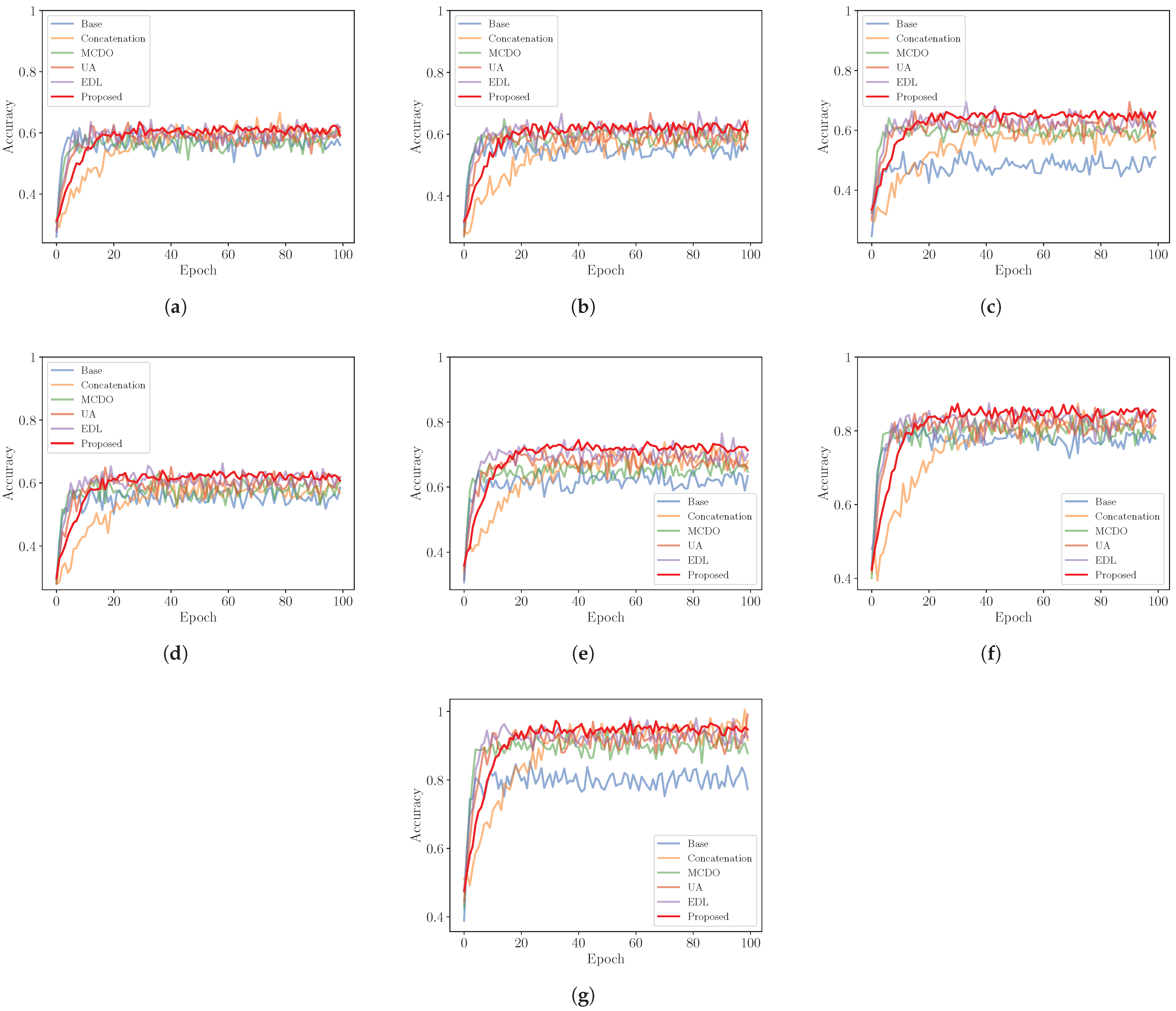
5.5. Convergence Evaluation

To evaluate the training efficiency of different models, we compare their convergence behaviors across multiple datasets, as illustrated in Figure 4. The evaluation includes BreakHis (with magnifications of $40\times$, $100\times$, $200\times$, and $400\times$), Oxford-IIIT, Chest X-ray, and Plant Leaf Disease datasets.

Convergence speed is measured by the number of epochs required for each model to reach a stable accuracy. Among the models, the base model exhibits the fastest convergence, followed by MCDO, EDL, and UA. The proposed method converges more slowly but still faster than the concatenation approach, which requires the most training epochs to stabilize. This trend is consistent across all datasets.

Although the proposed method converges more slowly, it consistently achieves the highest final performance across all datasets, followed by EDL, Concatenation, UA, MCDO, and Base. These results suggest that while faster-converging models such as Base and MCDO may offer early training efficiency, they tend to underperform in terms of final accuracy compared with slower-converging but more robust methods such as the proposed model and EDL.

Overall, these observations highlight a trade-off between convergence speed and model performance, underscoring the importance of selecting a model that aligns with the desired balance between training efficiency and classification reliability.

5.6. Ablation Study

To further validate the robustness and effectiveness of the proposed method, we conduct an ablation study focusing on two critical aspects: the uncertainty threshold and the model’s behavior under noisy input conditions. First, we examine the sensitivity of the model to the uncertainty threshold, which controls the confidence level required for making predictions. While the main results were obtained using a fixed threshold of $0.5$, we systematically varied this threshold from 0 to 1 to assess its influence on classification performance and model calibration. Second, we evaluate the model’s resilience to input corruption by introducing Gaussian noise with zero mean and increasing standard deviations (ranging from 0 to ${10}^9$) to one of the input views. This experiment simulates real-world scenarios with degraded or unreliable input and allows us to analyze how well the model maintains predictive accuracy and uncertainty estimation under challenging conditions.

5.6.1. Uncertainty Threshold

Figure 5 illustrates the classification accuracy of the proposed method across different real-world datasets as the uncertainty threshold varies from 0 to 1. Overall, the performance improves with increasing threshold values. At low thresholds (0 to $0.2$), most uncertain predictions are included, leading to a slight drop in accuracy. In contrast, at high thresholds ($0.8$ to 1), only high-confidence predictions are retained, resulting in improved accuracy at the cost of fewer predictions being made. The threshold of $0.5$ represents a balanced trade-off and is therefore used throughout the experiments in this study. Notably, the most significant accuracy gain is observed on the BreakHis dataset at $100\times$ magnification, while the gain is minimal on the Plant Leaf Disease dataset, likely due to differences in data noise and ambiguity.

5.6.2. Performance on Noisy Input

To evaluate the robustness of uncertainty-aware models under noisy conditions, we simulate a real-world scenario where one of the two input views is corrupted by additive Gaussian noise with zero mean and varying standard deviations (${10}^{-2}\le \sigma \le {10}^9$). Figure 6 presents the classification accuracy of four methods across four real-world datasets: BreakHis at $40\times$, $100\times$, $200\times$, and $400\times$ magnifications; Oxford-IIIT; Chest X-ray; and Plant Leaf Disease.

Across all datasets, the proposed method consistently achieves the highest accuracy under low to moderate noise levels ($\sigma \le {10}^3$). While all methods experience significant performance degradation as noise level increases, the proposed method shows the subtlest drop in accuracy. For example, on the BreakHis $200\times$ dataset (Figure 6c), the accuracy of the proposed method drops only modestly from $0.657$ ($\sigma =0$) to $0.620$ ($\sigma ={10}^3$), remaining significantly higher than MCDO ($0.350$), UA ($0.370$), and EDL ($0.390$) at the same noise level.

As the standard deviation increases beyond ${10}^3$, all models begin to show more pronounced degradation. Nevertheless, the proposed method continues to outperform the baselines. On the Chest X-ray dataset (Figure 6f), for example, it maintains an accuracy of $0.670$ at $\sigma ={10}^4$, compared with $0.470$ (EDL), $0.460$ (UA), and $0.440$ (MCDO). Even under extreme noise ($\sigma ={10}^9$), the proposed method retains a relatively stable accuracy of $0.270$, while MCDO, UA, and EDL drop below $0.200$.

These findings highlight the superior robustness of the proposed method against noisy inputs. By explicitly modeling belief, disbelief, and uncertainty through subjective logic, the model is better equipped to suppress the influence of corrupted features. Compared with MCDO, which relies on stochastic dropout sampling, UA, which focuses on uncertainty-aware feature weighting, and EDL, which estimates evidence-based distributions, the proposed approach provides a more principled mechanism for handling data uncertainty.

Overall, the proposed method offers a favorable trade-off between prediction accuracy and robustness, making it particularly suitable for real-world applications where sensor noise or corrupted data is common.

6. Conclusions

This paper introduces a pseudo-multiview learning framework that leverages subjective logic to fuse multiple feature representations at the evidence level, addressing the limitations of traditional concatenation-based fusion. By modeling belief, disbelief, and uncertainty, the proposed approach dynamically weights different feature views according to their reliability, enabling more robust and interpretable classification decisions. Experimental results across a range of real-world datasets validate the effectiveness of the method, showing consistent improvements in both AUC and accuracy over the base and concatenation models. Furthermore, comparative evaluations with state-of-the-art uncertainty-aware methods demonstrate the superior performance of the proposed framework, particularly in challenging scenarios.

In addition, ablation studies were conducted to analyze the influence of uncertainty threshold settings and the model’s behavior under noisy input conditions. The results reveal that the proposed method maintains high performance even when one input view is corrupted by noise, exhibiting stronger robustness than single-view uncertainty-aware approaches. This resilience highlights the advantage of leveraging multiple complementary views and fusing them at the evidence level.

However, the proposed method is not without limitations. First, although subjective logic offers a formal treatment of uncertainty, the model’s internal decision process remains difficult to interpret from a human-centric perspective, limiting transparency. Second, the evidence-based fusion process, particularly the estimation of Dirichlet parameters and variational modeling, introduces additional computational complexity compared with simpler fusion strategies. Third, the current framework assumes conditional independence between input views and does not explicitly model potential correlations, which may lead to suboptimal fusion when strong inter-dependencies exist. Addressing these limitations represents a promising direction for future research aimed at improving interpretability, efficiency, and fusion fidelity.