Abstract
This paper introduces an enhanced Iterative Finite Difference (IFD) method for efficiently solving strongly nonlinear, time-dependent problems. Extending the original IFD framework for nonlinear ordinary differential equations, we generalize the approach to address nonlinear partial differential equations with time dependence. An improved strategy is developed to achieve high-order accuracy in space and time. A finite difference discretization is applied at each iteration, yielding a flexible and robust iterative scheme suitable for complex nonlinear equations, including the Sine-Gordon, Klein–Gordon, and generalized Sinh-Gordon equations. Numerical experiments confirm the method’s rapid convergence, high accuracy, and low computational cost.
Keywords:
Sine-Gordon equation; Klein–Gordon equation; generalized Sinh-Gordon equation; higher-order approximation; finite difference discretization; order of convergence MSC:
65M06; 35G30
1. Introduction
We present an improved Iterative Finite Difference (IFD) method for efficiently solving highly nonlinear, time-dependent partial differential equations (PDEs). While the method is specifically developed for a class of nonlinear problems known as Gordon-type equations, it is also applicable to a broader range of nonlinear PDEs. Gordon-type equations, including Sine-Gordon, Klein–Gordon, and generalized Sinh-Gordon models, arise in various scientific and engineering disciplines. For example, Sine-Gordon equation is widely used in condensed matter and plasma physics, as well as nonlinear optics, to describe wave propagation and soliton dynamics, with applications ranging from Josephson junctions to optical fibers [1]. On the other hand, Klein–Gordon equation plays a central role in relativistic quantum mechanics and quantum field theory, particularly in modeling scalar particle dynamics [2]. Nevertheless, generalized Sinh-Gordon equation has notably several applications: in fiber optics, it models nonlinear wave propagation [3]; in condensed matter and plasma physics, it captures material behavior and wave instabilities [4]; and in nonlinear optics, it describes soliton formation and interactions [3]. It is also applied in biological systems, where it can model wave-like patterns and soliton behavior in complex biological environments [5]. Beyond their practical relevance, Gordon-type problems also serve as valuable benchmarks for evaluating and comparing numerical methods for nonlinear PDEs. The proposed IFD method addresses the challenges posed by such equations through an iterative finite difference framework capable of achieving high accuracy while maintaining computational efficiency.
A wide range of analytical and numerical methods have been proposed to tackle highly nonlinear problems. Among these techniques, we may cite wavelet-based approaches [6], integral solution methods using Green’s functions [7], and symmetry-based strategies such as the Lie-group shooting method [8]. In the context of finite difference schemes, Buckmire [9] employed Mickens’ nonstandard finite difference methods to solve several nonlinear boundary value problems, including bifurcation-type eigenvalue problems like those of Bratu and Gelfand type. Earlier work by Bank and Chart [10] introduced a multigrid continuation algorithm tailored to parameterized nonlinear elliptic systems. Continuation and multigrid strategies were further explored by Chan et al. [11] and Chang et al. [12] for nonlinear eigenvalue problems, while Fedoseyev et al. [13] developed continuation techniques for nonlinear elliptic PDEs discretized using multiquadratic methods. Additionally, Doedel et al. [14] contributed collocation-based approaches for continuation problems involving nonlinear elliptic PDEs. More recently, an improved IFD technique has been developed and studied in various nonlinear settings, showing promising results in terms of convergence and accuracy. The present work builds on this foundation and extends it to a broader class of nonlinear, time-dependent PDEs. The IFD method has been successfully applied to a variety of well-known nonlinear ordinary differential equations (ODEs) such as Bratu’s problem [15] and the Falkner–Skan problem [16].
Extending the IFD method to time-dependent nonlinear problems, particularly those of the Gordon-type, introduces additional challenges and opportunities. Several studies have explored such time-dependent nonlinear problems using various numerical and analytical techniques. For instance, Wazwaz [17] employed a modified decomposition method to treat nonlinear Klein–Gordon and Lane–Emden equations analytically. Guo et al. [2] applied the element-free kp–Ritz method to the nonlinear Klein–Gordon equation. In another study, Zhang and Ge [18] developed a high-order compact difference scheme for one-dimensional nonlinear advection–diffusion–reaction equations, including Burgers’ equation. Shukla and Tamsir [1] proposed a modified cubic B-spline differential quadrature method to solve the nonlinear sine–Gordon equation. Furthermore, Wazwaz [5] analyzed one- and two-soliton solutions of the sinh–Gordon equation in various dimensions. These works underscore the growing interest in efficient and accurate numerical schemes for solving nonlinear, time-dependent PDEs. In this context, the extension of the IFD method to Gordon-type equations provides a promising direction, offering both high accuracy and computational efficiency.
In this manuscript, we consider the following family of nonlinear problems, given by
subject to the boundary conditions
and the initial conditions
where is the wave displacement at point and time ; while is a nonlinear function of u, is a function of x and t, and k is a constant.
The general formulation of the above-mentioned problem given by Equations (1a)–(1e) covers a wide range of nonlinear problems well-known in the literature. One set of these famous problems is the various Gordon-type problems, which are obtained depending on the expression of and as follows:
- -
- In the case of: and We obtain the Sine-Gordon equation
- -
- In the case of: we obtain the Klein–Gordon equation with nonlinearity of order (for pratical applications, usually or 3)
- -
- In the case of: , We obtain the generalized Sinh-Gordon equation
The main contribution of this work is the development of an improved Iterative Finite Difference scheme for solving nonlinear time-dependent PDEs of the form (1a). This method extends earlier IFD techniques [16] designed for ODEs to a general framework suitable for strongly nonlinear PDEs, including the Sine-Gordon, Klein–Gordon, and generalized Sinh-Gordon equations. The proposed approach offers several advantages: it achieves high-order accuracy in both space and time through an iterative Taylor-based expansion of the nonlinear term; it converges rapidly, often within just a few iterations; it is computationally efficient, relying solely on standard finite difference operations without the need for solving nonlinear systems at each time step; and it is flexible, readily extendable to problems with variable coefficients. These strengths are demonstrated through a series of numerical experiments, which confirm the method’s accuracy, efficiency, and low computational cost. The approach is straightforward to implement, making it a practical and reliable tool for solving a wide class of nonlinear evolution equations.
This manuscript is structured as follows. Section 2 introduces the Time-dependent Iterative Finite Difference (TIFD) scheme for solving Gordon-type problems. Section 3, presents various numerical examples showcasing the accuracy of the scheme in computing solutions for different well-known nonlinear problems. Section 4 provides a summary of our findings, complemented by various graphical representations emphasizing the high precision achieved by the TIFD method, as we suggest as a further extension of the current work.
2. Iterative Finite Difference Method for Time-Dependent Problems
We assume that the exact solution is sufficiently smooth, i.e., so that all necessary partial derivatives up to order in both space and time exist and are continuous. This smoothness assumption ensures the validity of the Taylor series expansions and guarantees the consistency and accuracy of the finite difference approximations used in the proposed method.
First, we can rewrite Equation (1a) as
where
We consider a uniform mesh of size M over the space domain and a uniform mesh of size N over the time domain . We denote by and the step sizes of the mesh over the space domain and the time domain, respectively. Hence, the mesh nodes are denoted as
We also denote by U the numerical solution of the problem (1a)–(1e). We call the solution obtained by the iterative finite difference method at iteration n. Then, the discretization of Equation (5) at iteration n can be written as follows:
where
Now, we introduce the following quadratic approximation in function space of as a generalization of the Newton–Raphson–Kantorovich quasi-linear approximation [19], as follows:
Hence, (8) can be written as:
Similarly, the higher-order approximation of order p () for in function space can be written as:
with being the r-th derivative of with respect to u.
To ensure the validity of the approximation in Equation (11), we require that the nonlinear function be at least p-times continuously differentiable, i.e., , where p is the order of the expansion. This regularity ensures that the truncated Taylor series remains accurate and that the error introduced in the iterative scheme remains controlled.
Inserting the approximation (11) into the discretization (7) and re-arranging the terms, we obtain, for and :
For the sake of simplicity, we will be denoting as , and we use this notation to write the standard centred finite difference approximations of the second-order partial derivatives in space and in time for and , as:
substituting (13a) and (13b) in Equation (12) and solving for leads to
The boundary conditions for are discretized as:
while the initial conditions for are discretized as:
We note that (14e) is established by writing the expansion of , given that , as follows:
then substituting using the original problem (1a) as
in addition to the use of the initial conditions (1d).
We note that while Equations (1a)–(1e) is strictly valid for , we formally use it at in conjunction with the initial data to construct a second-order accurate approximation for . This practice is standard in time-stepping schemes and does not affect the accuracy or consistency of the numerical method.
It is interesting to highlight that the proposed iterative scheme (14a)–(14e) is simple in terms of implementation and is flexible in terms of application. The proposed scheme not only solves Gordon-type problems, but also applies to any other problem that can be formulated in the form of (1a)–(1e).
In summary, the TIFD scheme will be applied as follows:
- Given an initial guess for and (iteration 0);
- At iteration :
- First, compute the boundary values and , for , using the boundary conditions (14b) and (14c), respectively;
- Compute the and for using the initial conditions discretization given by Equations (14d) and (14e), respectively;
- Compute the remaining values of the solution for and using the TIFD iterative scheme (14a).
- Compute the solution at iteration using the same procedure as iteration n.
Furthermore, to ensure the convergence of the method, it is essential to choose an appropriate initial guess such as a simple quadratic polynomial function in space and time that satisfies the given boundary and initial conditions.
Remark 1.
The proposed method can be extended to problems where the coefficient k in Equationw (1a)–(1e) is a function of x and t, i.e., . In this case, the term is discretized pointwise, and the iterative structure of the scheme remains applicable. However, additional care may be required to ensure stability and maintain accuracy, particularly if varies significantly across the domain.
3. Computational Results
In this section, we evaluate the accuracy and efficiency of the proposed method using problems with known exact solutions. The maximum error between two consecutive iterations ( and ) is given by
To assess convergence, we define the iterative method as numerically converged when the infinity norm of the difference between two successive iterates satisfies
where is a prescribed tolerance. In our numerical experiments, we use , in line with the precision capabilities of the quadruple-precision arithmetic used throughout the computations.
We also compute the infinity norm of the error (difference between the exact solution u and the computed solution ) defined as:
to check the accuracy of the method.
Computation results are carried out using several examples for different values of approximation order p (in Equation (14a)) and different mesh sizes in space and time . In all the numerical examples presented in this section, the considered PDEs are solved on the domain . Furthermore, boundary conditions are applied for all , and the numerical solutions are computed over a uniform discrete mesh in both space and time. The results shown in the tables correspond to computations carried out on this domain using a finite number of time steps.
All computations were carried out using MATLAB R2024a with the Multiprecision Computing Toolbox (Advanpix, version 4.9.3.15018) [20], which enables highly accurate quadruple-precision arithmetic (up to the order of ) to guarantee the accuracy of the results.
Finally, we note also that we compute the order of convergence of the method for each case of . The order of convergence is computed as follows:
Assuming the rate of convergence of the method is r, we can write:
with being a positive constant.
Then, for simplicity reason, we call .
Hence,
which also means that:
Dividing (21) by (22), leads to
Then, applying the logarithm on both sides, we obtain
which implies that
3.1. Example 1: Sine-Gordon Equation
3.1.1. Simulation Results
We consider the Sine-Gordon equation problem (2) with :
which is known to have the following exact solution [1]:
under the following initial conditions
with boundary conditions taken from the exact solution (27).
In Table 1, we present the infinity norm of the error and the computation time for the solution pf the Sine-Gordon equation using different mesh sizes in space and time, and for order of approximation in the TIFD method. These results validate our proposed method since the computed solution converges to the exact solution. The aforementioned results also show that our method achieves high accuracy, even with a relatively coarse mesh size. Another powerful point about the method is its fast convergence, as the computation time is short even with refined meshes. The presented results of recording the CPU time of a computation performed simply using a regular laptop (Intel Core i7-7700HQ CPU—2.80 GHz) exhibited in the aforementioned Table 1 affirm that the method is highly efficient as it converges to an exact solution in less than 4 s with the use of quadruple precision and mesh size .

Table 1.
Infinity norm of the error for the solution pf the Sine-Gordon Equation (26), for different mesh sizes using an approximation order .
Moreover, looking at the computation results in Table 2 of the order of convergence for all three cases of , it is confirmed that the convergence is of order for all three cases. Furthermore, we note that the proposed method has low computation cost as it converges in iterations when , and in only iterations in the case of .
Table 2.
Infinity norm of the error at each iteration for the solution of the Sine-Gordon Equation (26) and order of convergence, for different approximation orders and mesh size .
Furthermore, for the completeness of the study, in Figure 1, we exhibit a surface plot of the computed solution (left) and a surface plot of the absolute error (right) for mesh size . The results are in agreement with the results published in [1], however, the method proposed in this manuscript provides more accurate results with low computation cost.

Figure 1.
Computed solution (left) pf the Sine-Gordon Equation (26) and its error (right) for mesh size (, ).
3.1.2. Comparative Analysis & Validation
To further evaluate the accuracy and efficiency of the proposed Iterative Finite Difference Method, we compare our results with those reported in the literature for the same problem setup, for . In particular, we consider the works of Shukla and Tamsir [1], Mittal and Bhatia [21], and Dehghan and Shokri [22], where various numerical techniques were applied to the one-dimensional nonlinear Sine-Gordon equation. In our approach, using a mesh size of , we obtained an norm of the error equal to . For comparison, the corresponding errors reported in [1,21,22] are , , and , respectively. Furthermore, our method converges in only 4 iterations and completes the computation in just 0.26 s (on the processor specified at the beginning of this section). A summary of this comparison is presented in Table 3, which clearly illustrates the competitive performance of our method in terms of both accuracy and computational cost.
Table 3.
Comparison of norm error for the Sine-Gordon Equation (26) with other numerical methods for mesh size (, ).
3.2. Example 2: Klein–Gordon Equation with Cubic Nonlinearity
We consider the Klein–Gordon Equation problem (3) with , , , , and :
with initial conditions
In this case, the problem is known to have the following exact solution [2,23]:
with , , and .
In Table 4, we present the infinity norm of the error for the solution of Klein–Gordon equation with cubic nonlinearity. In this case also, the method converges in only iterations in the case of . Also, in Table 5, we present the computation of the order of convergence for the cases of and confirming again that the convergence is of order . We note that for the convergence is extremely fast (converges at the third iteration with an error of order < considered 0 for quadruple precision) so that the convergence rate can’t be computed (according to Formula (19), the error needs to be non-zero for at least three iterations to numerically compute the order of convergence).
Table 4.
Infinity norm of the error for the solution of the Klein–Gordon Equation (28), for different mesh sizes using an approximation order .
Table 5.
Infinity norm of the error at each iteration for the solution of the Klein–Gordon Equation (28) and order of convergence, for the different approximation orders and mesh size .
Again, we exhibit in Figure 2, surface plots of the computed solution and the absolute error resealing a perfect agreement with the results published in [2] as well.
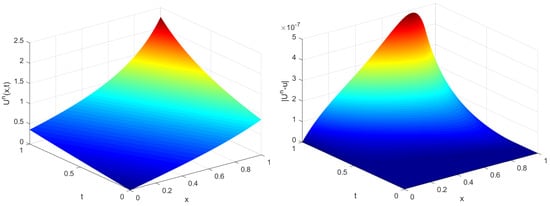
Figure 2.
Computed solution (left) of the Sine-Gordon Equation (28) and its error (right) for mesh size (, ).
3.3. Example 3: Sinh-Gordon Equation
We consider the generalized Sinh-Gordon equation problem (4) with , , , and :
which has the following exact solution:
under the following initial conditions
and boundary conditions
with taken from substituting the exact solution (31) into the original problem (30):
Similarly to the previous examples, in Table 6 and Table 7, we present the computational results for the Sinh-Gordon equation. It is shown again that the method performs efficiently and converges fast in the case of , and even faster in the cases and . The order of convergence is also confirmed to be for all the considered cases .
Table 6.
Infinity norm of the error for the solution pf the Sinh-Gordon Equation (30), for different mesh sizes using an approximation order .
Table 7.
Infinity norm of the error at each iteration for the solution of Sinh-Gordon Equation (30) and order of convergence, for different approximation orders and mesh size .
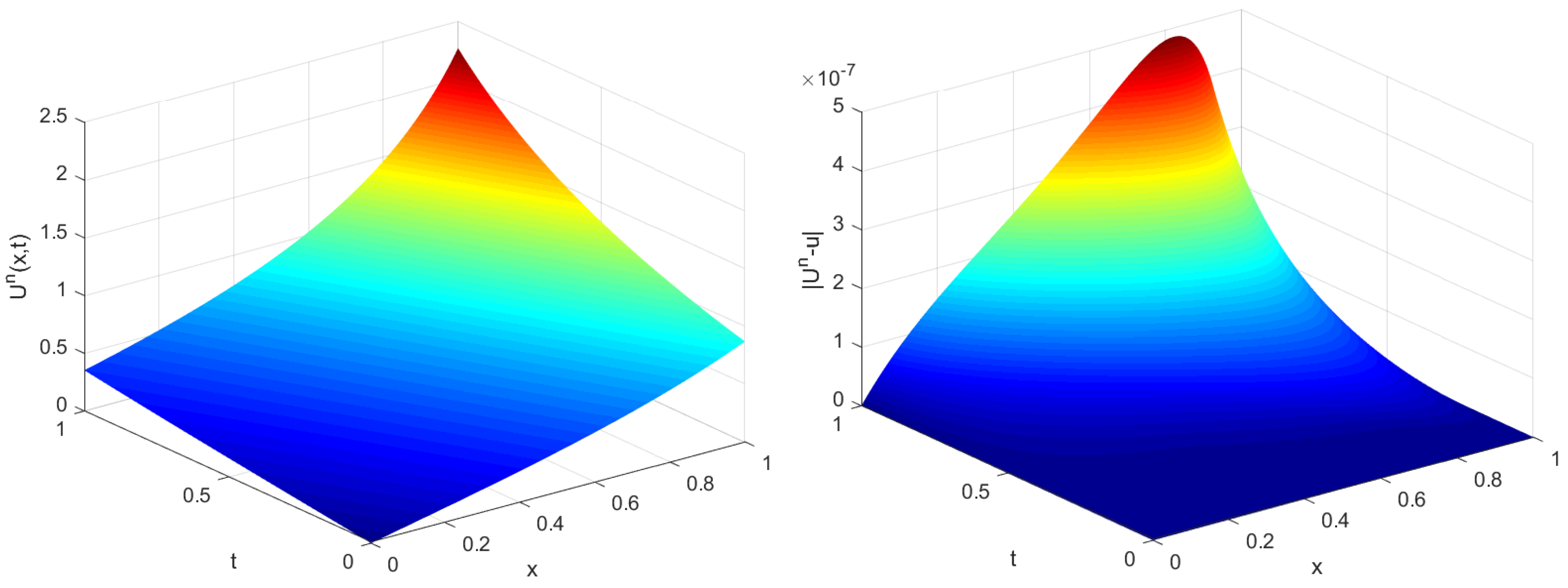
Finally, we exhibit in Figure 3 surface plots of the computed solution and the absolute error for the case of the sinh-Gordon equation.

Figure 3.
Computed solution (left) pf the Sine-Gordon Equation (30) and its error (right) for mesh size (, ).
3.4. Example 4: Another Example of the Sinh-Gordon Equation
We consider the generalized Sinh-Gordon equation problem (4) with , , , and :
which has the following exact solution:
under the following initial conditions
and boundary conditions
with obtained from the original problem (32) by substituting the exact solution (33), which leads to:
Similarly to the previous examples, in Table 8 and Table 9, we present the computational results for another case pf the Sinh-Gordon equation. Our results agree with the observation drawn from the previous examples, that the method is accurate, computationally efficient, and that the order of convergence depends on the approximation order p. It is again confirmed to be for all the considered cases .
Table 8.
Infinity norm of the error and computation time for the solution pf the Sinh-Gordon Equation (32), for different mesh sizes using an approximation order .
Table 9.
Infinity norm of the error at each iteration for the solution pf the Sinh-Gordon Equation (32) and order of convergence, for different approximation orders and mesh size .
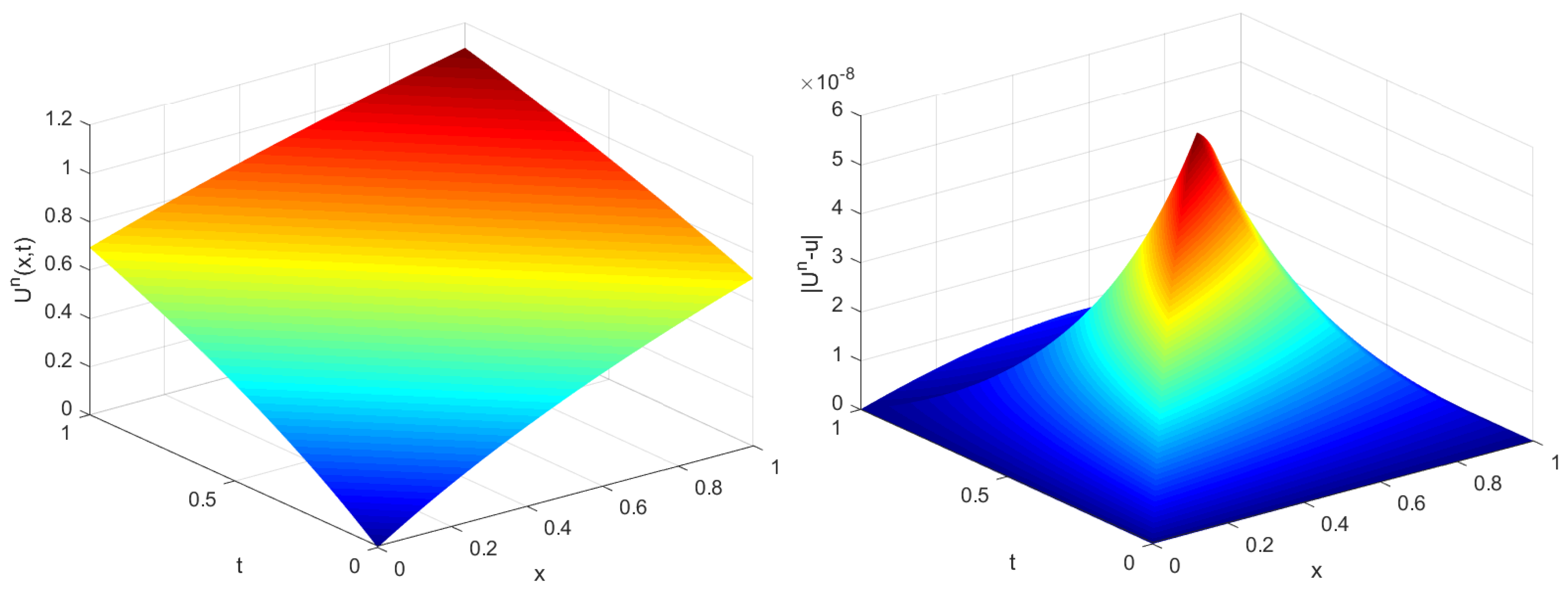
Finally, we exhibit in Figure 4 surface plots of the computed solution and the absolute error for the case of the Sinh-Gordon Equation (32).
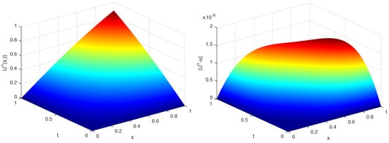
Figure 4.
Computed solution (left) of the Sinh-Gordon Equation (32) and its error (right) for mesh size (, ).
As an ending remark, we note that several of the results reported in Table 1, Table 4, Table 6 and Table 8 correspond to simulations with unequal spatial and temporal step sizes (). These cases confirm that the proposed method remains accurate and convergent under nonuniform discretizations, consistent with the theoretical expectations. For visual clarity, the figures accompanying the examples were generated using equal mesh sizes (); this was a deliberate technical choice made to facilitate straightforward comparisons between methods and grid levels. Importantly, the method itself does not require the spatial and temporal step sizes to be equal.
4. Conclusions
In this manuscript, we presented an improved high-order iterative finite difference method for solving a class of strongly nonlinear, time-dependent partial differential equations. The method was tested on smooth benchmark problems with known exact solutions, and the results provided strong numerical evidence of its accuracy, fast convergence, and low computational cost. We note, however, that the test cases considered involve smooth solutions. To fully assess the method’s robustness (particularly for dispersive PDEs with oscillatory or less regular behavior), further studies are needed. As such, future work will focus on applying the method to more complex, real-world problems and assessing its effectiveness in those settings. In addition, it may include a sensitivity analysis with respect to perturbations in the initial and boundary conditions, in order to evaluate the method’s robustness in the presence of uncertainty or noise in the input data. Furthermore, a rigorous analysis of convergence and stability could also be the objective of a future study building on the present numerical results.
Author Contributions
Conceptualization, M.B.-R. and H.T.; Methodology, M.B.-R. and H.T.; Software, M.B.-R.; Validation, M.B.-R.; Formal analysis, H.T.; Investigation, M.B.-R.; Data curation, H.T.; Writing—original draft, M.B.-R.; Writing—review & editing, H.T.; Visualization, H.T.; Supervision, H.T.; Project administration, H.T. All authors have read and agreed to the published version of the manuscript.
Funding
The current research did not receive any external funding.
Data Availability Statement
The original contributions presented in this study are included in the article. Further inquiries can be directed to the corresponding author.
Conflicts of Interest
The authors declare no conflicts of interest.
Abbreviations
The following abbreviations are used in this manuscript:
| IFD | Iterative Finite Difference |
| TIFD | Time-dependent Iterative Finite Difference |
| ODE | Ordinary Differential Equation |
| PDE | Partial Differential Equation |
References
- Shukla, H.S.; Tamsir, M. Numerical solution of nonlinear sine–Gordon equation by using the modified cubic B-spline differential quadrature method. Beni-Suef Univ. J. Basic Appl. Sci. 2018, 7, 359–366. [Google Scholar] [CrossRef]
- Guo, P.F.; Liew, K.M.; Zhu, P. Numerical solution of nonlinear Klein–Gordon equation using the element-free kp-Ritz method. Appl. Math. Model. 2015, 39, 2917–2928. [Google Scholar] [CrossRef]
- Ali, K.; Wazwaz, A.; Osman, M.S. Optical soliton solutions to the generalized nonautonomous nonlinear Schrodinger equations in optical fibers via the sine-Gordon expansion method. Optik 2020, 208, 164132. [Google Scholar] [CrossRef]
- Alzaleq, L.; Al-zaleq, D.; Alkhushayni, S. Traveling Waves for the Generalized Sinh-Gordon Equation with Variable Coefficients. Mathematics 2022, 10, 822. [Google Scholar] [CrossRef]
- Wazwaz, A.-M. One and two soliton solutions for the sinh–Gordon equation in (1 + 1), (2 + 1) and (3 + 1) dimensions. Appl. Math. Lett. 2012, 25, 2354–2358. [Google Scholar] [CrossRef]
- Liu, X.; Wang, J.; Zhou, Y. Wavelet solution of a class of two-dimensional nonlinear boundary value problems. Comput. Model. Eng. Sci. 2013, 92, 493–505. [Google Scholar]
- Mohsen, A. On the integral solution of the one-dimensional Bratu problem. J. Comput. Appl. Math. 2013, 251, 61–66. [Google Scholar] [CrossRef]
- Abbasbandy, S.; Hashemi, M.; Liu, C. The Lie-group shooting method for solving the Bratu equation. Commun. Nonlinear Sci. Numer. Simul. 2011, 16, 4238–4249. [Google Scholar] [CrossRef]
- Buckmire, R. Applications of Mickens finite differences to several related boundary value problems. Adv. Appl. Nonstandard Finite Differ. Schemes 2005, 1, 47–87. [Google Scholar]
- Bank, R.; Chart, T. PLTMGC: A multi-grid continuation program for parameterized nonlinear elliptic systems. SIAM J. Stat. Sci. Comput. 1986, 7, 540–559. [Google Scholar] [CrossRef]
- Chan, T.; Keller, H. Arc-length continuation and multigrid techniques for nonlinear elliptic eigenvalue problems. SIAM J. Sci. Stat. Comput. 1982, 3, 173–194. [Google Scholar] [CrossRef]
- Chang, S.; Chien, C. A multigrid-lanczos algorithm for the numerical solutions of nonlinear eigenvalue problems. Int. J. Bifurc. Chaos 2003, 13, 1217–1228. [Google Scholar] [CrossRef]
- Fedoseyev, A.; Friedman, M.; Kansa, E. Continuation for nonlinear elliptic partial differential equations discretized by the multiquadratic method. Int. J. Bifurc. Chaos 2000, 10, 481–492. [Google Scholar] [CrossRef]
- Doedel, E.; Sharifi, H. Collocation methods for continuation problems in nonlinear elliptic PDEs. Notes Numer. Fluid Mech. 2000, 74, 105–118. [Google Scholar]
- Temimi, H.; Ben-Romdhane, M.; Baccouch, M.; Musa, M. A two-branched numerical solution of the two-dimensional Bratu’s problem. Appl. Numer. Math. 2020, 153, 202–216. [Google Scholar] [CrossRef]
- Temimi, H.; Ben-Romdhane, M. Numerical solution of Falkner–Skan equation by iterative transformation method. Math. Model. Anal. 2018, 23, 139–151. [Google Scholar] [CrossRef]
- Wazwaz, A.-M. The modified decomposition method for analytic treatment of differential equations. Appl. Math. Comput. 2006, 173, 165–176. [Google Scholar] [CrossRef]
- Zhang, L.; Ge, Y. Numerical solution of nonlinear advection diffusion reaction equation using high-order compact difference method. Appl. Numer. Math. 2021, 166, 127–145. [Google Scholar] [CrossRef]
- Bellman, R.E.; Kalaba, R.E. Quasilinearization and Nonlinear Boundary-Value Problems; American Elsevier Publishing Company: New York, NY, USA, 1965. [Google Scholar]
- Advanpix LLC. Multiprecision Computing Toolbox for MATLAB R2018a (Version 4.9.3.15018); Advanpix LLC.: Yokohama, Japan, 2025. [Google Scholar]
- Mittal, R.C.; Bhatia, R. Numerical solution of nonlinear sine–Gordon equation by modified cubic B-spline collocation method. Int. J. Partial. Differ. Equ. 2014, 2014, 343497. [Google Scholar] [CrossRef]
- Dehghan, M.; Shokri, A. A numerical method for one dimensional nonlinear sine–Gordon equation using collocation and radial basis functions. Numer. Methods Partial. Differ. Equ. 2008, 24, 687–698. [Google Scholar] [CrossRef]
- Kaya, D.; El-Sayed, S.M. A numerical solution of the Klein-Gordon equation and convergence of the decomposition method. Appl. Math. Comput. 2004, 156, 341–353. [Google Scholar] [CrossRef]


Disclaimer/Publisher’s Note: The statements, opinions and data contained in all publications are solely those of the individual author(s) and contributor(s) and not of MDPI and/or the editor(s). MDPI and/or the editor(s) disclaim responsibility for any injury to people or property resulting from any ideas, methods, instructions or products referred to in the content. |
© 2025 by the authors. Licensee MDPI, Basel, Switzerland. This article is an open access article distributed under the terms and conditions of the Creative Commons Attribution (CC BY) license (https://creativecommons.org/licenses/by/4.0/).