Abstract
Fractional-order four-wing (FO 4-wing) systems are of significant importance due to their complex dynamics and wide-ranging applications in secure communications, encryption, and nonlinear circuit design, making their control and stabilization a critical area of study. In this research, a novel model-free finite-time flexible sliding mode control (FTF-SMC) strategy is developed for the stabilization of a particular category of hyperchaotic FO 4-wing systems, which are subject to unknown uncertainties and input saturation constraints. The proposed approach leverages fractional-order Lyapunov stability theory to design a flexible sliding mode controller capable of effectively addressing the chaotic dynamics of FO 4-wing systems and ensuring finite-time convergence. Initially, a dynamic sliding surface is formulated to accommodate system variations. Following this, a robust model-free control law is designed to counteract uncertainties and input saturation effects. The finite-time stability of both the sliding surface and the control scheme is rigorously proven. The control strategy eliminates the need for explicit system models by exploiting the norm-bounded characteristics of chaotic system states. To optimize the parameters of the model-free FTF-SMC, a deep reinforcement learning framework based on the adaptive dynamic programming (ADP) algorithm is employed. The ADP agent utilizes two neural networks (NNs)—action NN and critic NN—aiming to obtain the optimal policy by maximizing a predefined reward function. This ensures that the sliding motion satisfies the reachability condition within a finite time frame. The effectiveness of the proposed methodology is validated through comprehensive simulations, numerical case studies, and comparative analyses.
Keywords:
fractional-order 4-wing systems; sliding mode control; finite-time stability; Lyapunov stability theory MSC:
26A33; 93C10; 93D05; 93D15; 93D40
1. Introduction
Chaotic systems and uncertain nonlinear systems have been widely studied due to their complex and unpredictable behavior, with applications in secure communication, cryptography [1,2], robotics [3,4,5], autonomous systems [6,7,8] and nonlinear control [9,10,11]. Among these, four-wing chaotic systems represent a class of multi-scroll attractors that exhibit intricate dynamical patterns with four distinct wings in their phase space [12]. Traditionally, these systems are formulated using integer-order differential equations, which capture essential chaotic properties such as sensitivity to initial conditions and ergodicity. However, integer-order models have limitations in accurately representing real-world phenomena, as they lack memory effects and flexibility in controlling chaotic behavior [13,14].
To overcome these limitations, fractional-order four-wing chaotic systems (FO 4-wing CSs) have been introduced, extending traditional models by incorporating fractional derivatives that account for memory and hereditary properties. Fractional calculus enhances the system’s complexity, providing richer dynamical behaviors, greater unpredictability, and improved control, making them highly suitable for secure communication, image encryption, and biological modeling [15,16]. Moreover, the additional degrees of freedom in fractional-order systems enable finer tuning of chaotic dynamics, improving performance in cryptographic applications and synchronization tasks. As a result, fractional-order four-wing CSs have gained significant attention in nonlinear science, offering a more generalized and realistic approach to modeling chaotic behaviors [17].
Control of FO 4-wing CSs is crucial due to their extreme sensitivity to initial conditions and complex, unpredictable behavior. Without proper control mechanisms, these systems can exhibit unbounded chaos, making them impractical for real-world applications [18]. Chaos control ensures that the system operates within desired constraints, enabling its use in practical applications such as secure communication, robotics, power systems, and biomedical engineering. For instance, in secure communication, controlling chaos allows for effective signal modulation, while in engineering systems, stabilization of chaotic behaviors is necessary to prevent instability [19].
Motivated by these challenges and opportunities, researchers focus on developing advanced control strategies for FO 4-wing CSs. Furthermore, since fractional-order systems exhibit richer dynamics and additional tunable parameters compared to integer-order systems, their control requires specialized techniques tailored to fractional calculus [20]. The ability to effectively manage chaos in such systems paves the way for more robust cybersecurity, advanced signal processing, and next-generation cryptographic protocols. Hence, the study of control and synchronization in fractional-order four-wing chaotic systems remains an active and highly relevant research area, with significant implications for both theoretical advancements and technological innovations [21].
Numerous control strategies have been developed to address undesirable dynamics in nonlinear systems. These approaches encompass optimal control [22], fuzzy control [23], proportional–integral–derivative (PID) methods [24], adaptive control [25], backstepping techniques [26], sliding mode control (SMC) [27,28], impulsive control [29], model-free control [30], neural networks [31,32], and so on. Among these, SMC has gained significant attention due to its robustness to uncertainties, ease of implementation, high precision, and adaptability.
In recent years, many researchers have introduced diverse SMC-based approaches for achieving synchronization in fractional-order (FO) delayed systems. Specifically, in [33], a finite-time second-order SMC approach was proposed for nonlinear FOSs, incorporating a fractional switching surface to ensure finite-time reachability. The method adapts LQR performance to improve transient response, with stability conditions derived using Lyapunov theory and LMIs. The authors of [34] proposed a fractional-order SMC scheme for free-floating space manipulators to address uncertainties, disturbances, and input saturation. In [35], a sliding mode controller for fractional-order uncertain linear systems with Caputo derivatives was designed. Using LMIs and FO stability theory, sufficient conditions for asymptotic stability were derived, and an adaptive law was introduced to handle unknown uncertainty bounds. In [36], SMC methods were applied to integer- and fractional-order systems to enhance control performance, robustness, and accuracy. That study underscores the potential of fractional-order modeling and control techniques in advancing modern control engineering. The authors of [37] proposed a fractional-order fuzzy sliding mode controller with online FO reinforcement learning for unknown MIMO nonlinear systems. The method employs TSK fuzzy neural networks to approximate control components and a value function, while an adaptive fractional-order Levenberg–Marquardt learning mechanism optimizes parameters online. In [38], the chaotic behavior of a 4D FO memristive system was investigated, revealing enriched dynamics through bifurcation diagrams, Lyapunov exponents, and phase portraits. A single-state FOSMC was designed to stabilize the system at equilibrium points, validated via numerical simulations and microcontroller-based experiments. In [39], chaos in the fractional-order Bloch equation, with and without delay, was studied using a sliding mode controller. The controller’s robustness was tested under uncertainties and disturbances for both commensurate and incommensurate systems, while theoretical aspects like solution existence, uniqueness, and stability were analyzed. In [40], a robust terminal SMC with a novel fractional-order sliding surface and time-varying gain was proposed for nonlinear systems. The time-varying gain reduces control input amplitude initially and increases precision near a steady state, addressing limitations of constant-gain approaches. The authors of [41] studied SMC for FOSs with disturbances, extended a fractional power-rate inequality to a more general form, and proposed a modified fractional integral SMC method, increasing the sliding mode surface’s degree of freedom. In [42], two control strategies for discrete FO systems were proposed—discrete SMC and adaptive SMC—for handling unknown time-varying parameters. Stability and reachability were proven using Lyapunov theory, ensuring finite-time quasi-sliding mode convergence. In [43], the Mittag-Leffler synchronization problem for a class of FOSs was addressed under unknown disturbances. An adaptive SMC method was proposed, incorporating an FO term to enhance convergence rate, reduce chattering, and improve tracking accuracy and robustness. In [44], a model-free -SMC methodology was proposed for synchronizing chaotic FO memristive neural networks with delays and input saturation. A two-level -SMC was designed using fractional-order Lyapunov stability theory, ensuring finite-time synchronization and robustness against uncertainties.
However, the referenced studies demonstrate several notable shortcomings, which can be summarized as follows.
- Current research frequently depends predominantly on either linear or nonlinear elements when proposing control strategies, which restrict the overall robustness and adaptability of the methods.
- The application of SMC techniques is often associated with undesirable chattering effects, which are impractical in real-world scenarios.
- A significant portion of these studies oversimplifies system models by disregarding critical factors such as uncertainties, external disturbances, and input constraints, all of which play a vital role in practical systems.
- Nearly all of these approaches determine control parameters through conventional trial-and-error methods during simulations, which may not yield optimal or reliable results.
- Additionally, many of these studies fail to address or ensure finite-time stability, a crucial requirement for achieving rapid convergence and enhanced performance in dynamic systems.
To tackle the identified challenges, this study introduces an innovative model-free finite-time flexible SMC (FTF-SMC) approach. The proposed technique is designed to create a chattering-free FTF-SMC strategy that is both dynamic and resilient against uncertainties, external disturbances, and input saturation. The methodology begins with the introduction of a primary sliding surface. Then, a dynamic-free control law is formulated, ensuring robustness against system uncertainties, and saturation input. The finite-time asymptotic stability of both surfaces is rigorously established. Additionally, to enhance the optimization of FTF-SMC parameters, adaptive dynamic programming (ADP) is adopted to dynamically adjust control parameters.
The key contributions and innovations of this research are outlined below.
- I.
- Introduction of a Novel Control Framework: This work presents a model-free FTF-SMC framework specifically tailored for control and stabilization of a FO 4-wing CS with input saturation.
- II.
- Finite-Time control Assurance: The proposed control strategy ensures finite-time control for a FO 4-wing CS, effectively addressing input saturation, and system uncertainties that have posed challenges in prior studies.
- III.
- System-Agnostic Design: The control laws are formulated to be independent of the specific system functions, leveraging the norm-boundedness property of chaotic system states. This enhances the methodology’s applicability across diverse chaotic systems.
- IV.
- Optimization via Adaptive Dynamic Programming (ADP) Algorithm: The study employs the ADP algorithm to fine-tune control parameters of the model-free FTF-SMC. The neural networks (action and critic networks) of ADP are trained in such a way that enhances controller adaptability by maximizing a reward signal.
- V.
- Comprehensive Validation: The efficacy of the proposed control strategy is validated through extensive simulations and two numerical case studies, demonstrating its practical relevance in engineering applications. A detailed comparison with an existing SMC method is also conducted, highlighting the superior performance of the proposed approach in terms of faster convergence, and enhanced robustness against uncertainties and disturbances. This comparative analysis underscores the advancements achieved by the proposed methodology over traditional SMC techniques.
- VI.
- Real-World Applicability: The robustness of the proposed FTF-SMC method in managing chaotic dynamics and input saturation highlights its potential for real-world engineering applications, particularly in complex system control.
The remainder of the paper is structured as follows. Section 2 outlines foundational concepts related to fractional-order systems and stability theorems. Section 3 defines the problem statement and details the novel model-free FTF-SMC technique for controlling a FO 4-wing CS, presented in two steps. Section 4 explains the adaptive dynamic programming (ADP) algorithm and its role in optimizing controller parameters. Section 5 provides numerical simulations and case studies to validate the analytical findings. Finally, Section 6 concludes the paper with a discussion of the results and their implications.
2. Preliminary Concepts
Definition 1.
[45] Consider a continuous function defined on a set of real numbers (). The Riemann–Liouville fractional integral of is defined as follows:
Here, signifies the initial time point and represents the order of integration. The term refers to the gamma function.
Definition 2.
[45] Consider a continuous function defined over the domain of real numbers. The Caputo fractional-order derivative of is defined as follows:
In the subsequent sections of this work, the Caputo derivative will be represented using the notation . Below are some of the key properties associated with this definition [46]:
- I.
- If , and belongs to the space , then the following holds:
- II.
- Suppose , and is a constant. In this case,
Theorem 1.
[47] Let , and consider the fractional-order system , which satisfies the Lipschitz condition and has an equilibrium point at . Suppose there exists a Lyapunov function that satisfies the following conditions:
where
, , and
are positive constants. Under these conditions, the equilibrium point of the fractional-order system
will demonstrate (asymptotic) stability in accordance with the Mittag-Leffler framework.
Theorem 2.
[48] Let , and consider the fractional-order system , which satisfies the Lipschitz condition and has an equilibrium point at . Suppose there exists a Lyapunov function that satisfies the following conditions:
where
, , and are positive constants, , and . In this case, the system is considered finite-time stable. Also, the system will reach a stabilized state within a finite time T, which is given by:
3. Problem Formulation and Design of Finite-Time PID Sliding Mode Control
The core challenge addressed in this work revolves around the stabilization and control of a FO 4-wing chaotic system with time delays, operating under the influence of unknown dynamics and external uncertainties. The objective is to design a robust finite-time control strategy, specifically leveraging flexible sliding mode control (SMC), to ensure the system achieves stability within a finite time frame. This involves addressing the complexities introduced by the chaotic nature of the system, as well as mitigating the effects of uncertainties and disturbances.
3.1. Problem Statement
In recent studies [18,19], a four-dimensional fractional-order four-wing chaotic system has been proposed, extending the principles of chaotic dynamics to systems. Here the mathematical representation of this four-dimensional FO 4-wing chaotic system with time delays is given by the following equations:
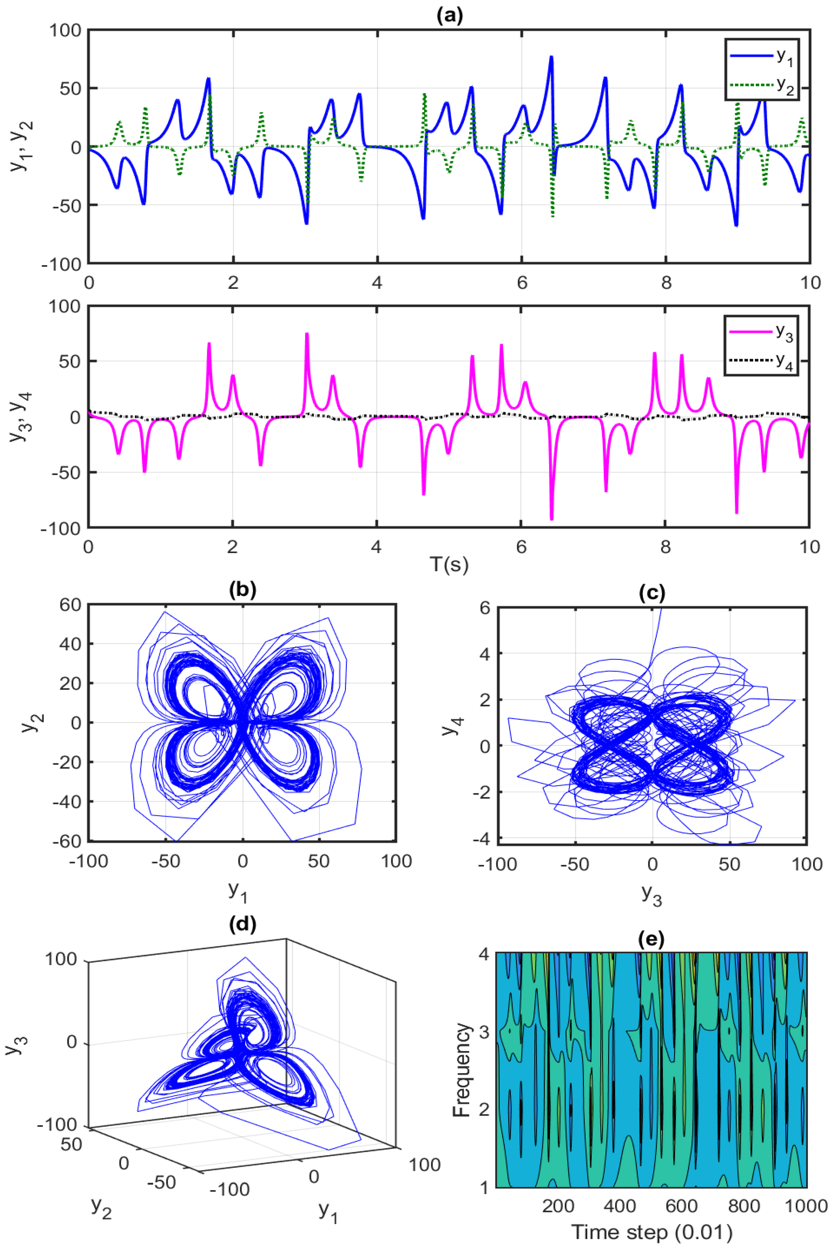
Here, represents the state trajectories of the system, denotes the fractional order of the derivative, and for , are continuous functions. The FO 4-wing CS (10) displays chaotic and unpredictable behavior when the parameters are set to , , , and . Using the initial conditions and , along with , the dynamic behavior of the FO 4-wing CS (10) is illustrated in Figure 1.

Figure 1.
Investigating chaotic dynamics in the FO 4−wing CS (10) at = 0.95. (a) Trajectories of the system states (10); (b) state space; (c) state space; (d) 3-dimensional state space; (e) contour plot view.
The hyper-chaotic attractors of the FO 4-wing CS (10) are distinctly illustrated in subfigures Figure 1a through Figure 1d. Also, the contour plot of the hyper-chaotic FO 4-wing attractor in the 2D plane (Figure 1e) reveals tightly wound spirals near its core, while chaotic, elongated patterns extend outward. The contours appear irregular, looping, and fragmented, highlighting the system’s inherent chaotic behavior.
Proceeding with the effort to tackle the stabilization problem for the FO 4-wing CS (10), the following FO 4-wing CS with control input is introduced:
where for are defined in the FO 4-wing CS (10) and the terms represent the uncertainties and external disturbances impacting the FO 4-wing CS. These components will be discussed in detail in later sections. Additionally, denotes the input control, considered:
where denotes the system’s input gain function, which is assumed to be invertible. Also:
And:
Here, and represent the upper bounds of the saturation relation, while and denote the lower bounds. Additionally, signifies the slope of the saturation.
Assumption 1.
The trajectories of system states in the FO 4-wing CS (11) are typically confined to specific regions of phase space [49,50], due to the irregular attractors generated by chaotic dynamics. Consequently, there exist positive constants and that satisfy the norm-bounded conditions described in the following relation:
Furthermore, it is assumed that the uncertainty and external disturbance terms are bounded in magnitude. Therefore, there exists a positive constant such that the following condition holds:
Thus, as a result from relations (15) and (16) one gets:
Assumption 4.
Guaranteeing the boundedness of the controller is a fundamental necessity to ensure practical and implementable control inputs. However, achieving this objective is a non-trivial task. As a result, the terms , must remain bounded. Consequently, there exist positive real numbers that satisfy the following conditions:
3.2. Design of the Finite-Time Flexible SMC
As an initial step to stabilize the chaotic FO 4-wing CS (10), the following steady-state (SS) formulation is designed in the first phase:
in which , , , and are positive real numbers and , and .
When the sliding motion is achieved, it is well established that the condition is met. As a result,
Theorem 3.
The dynamic equation describing the sliding surface dynamics (Equation (22)) will demonstrate stability, and the states of the FO 4-wing CS (Equation (11)) will asymptotically approach the origin in finite time.
Proof of Theorem 3.
Let us have the following Lyapunov candidate for and :
With the operating FO derivative from (23), we obtain:
Replacing from (22) in Equation (24), one obtains:
Therefore, according to Equation (26), the inequality holds asymptotically. Consequently, the stability conditions outlined in Theorem 1 are satisfied, ensuring the asymptotic stability of the SS dynamics (22).
For finite-time stability,
where . Thus,
Therefore, according to Theorem 2, the states converge to stability within a finite time . This concludes the proof. □
Remark 1.
The dynamic sliding surface is motivated by the need to enhance flexibility and adaptability in controlling complex nonlinear systems, especially those with uncertainties and time delays. Unlike classical fixed sliding surfaces, which are predefined and static, the dynamic sliding surface evolves with the system’s states and control inputs, allowing real-time adjustment to changing system dynamics. This adaptability improves robustness by mitigating chattering effects and providing smoother control actions, which in turn better handle parameter variations and external disturbances. Moreover, the dynamic structure facilitates finite-time convergence by incorporating system feedback more effectively, thus ensuring faster and more reliable stabilization compared to traditional sliding surfaces that may struggle under high uncertainty or nonlinearities.
Here, a novel dynamic-free flexible control strategy is presented as follows:
where , , , , and are positive finite real numbers and , and . Figure 2 illustrates the structure of the proposed controller.
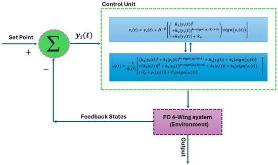
Figure 2.
Block diagram of the proposed model-free FTF-SMC.
The theoretical validation of the proposed controller implemented for the FO 4-wing CS (30) is as follows.
Theorem 4.
Consider the FO chaotic four-wing system (11). By applying the control strategy (30), the trajectories of the FO chaotic four-wing system (11) will achieve finite-time asymptotic stability.
Proof of Theorem 4.
Consider the following Lyapunov candidate, for and ,
By taking FO derivative from (31), one gets:
Replacing from (21) in Equation (32), one obtains:
Now, inserting from (11) in Equation (33), we have:
Referring to Equations (17) and (18) and using from (30), one obtains in (35):
Now, by some simplifications,
Therefore, according to Equation (37), the inequality holds asymptotically. Consequently, the stability conditions outlined in Theorem 1 are satisfied, ensuring the asymptotic stability of the FO 4-wing CS (11).
For finite-time stability,
where . Thus,
Thus, according to Theorem 2, for 4, the states converge to stability point within a finite time . This concludes the proof. □
Remark 2.
The stability analysis based on the fractional-order Lyapunov approach in this work is moderately conservative, primarily due to the boundedness assumptions on disturbances and initial conditions; however, the use of fractional calculus and the adaptive, model-free nature of the proposed finite-time flexible sliding mode control significantly reduce conservativeness compared to traditional methods. There is an inherent trade-off between convergence speed and robustness: faster convergence typically demands higher control gains, which can amplify chattering and reduce robustness, especially under input saturation constraints, but this is mitigated here by the flexible sliding surface design and the adaptive dynamic programming scheme that tunes control inputs online. The fractional-order Lyapunov framework effectively handles external disturbances and time-varying delays provided they remain bounded and their rates of change satisfy specific constraints. Disturbances are accounted for within the Lyapunov derivative bounds, ensuring ultimate boundedness, while time delays are managed via delay-dependent stability conditions embedded in the fractional calculus setting. Overall, while perfect disturbance rejection and delay compensation are not guaranteed, the method offers a robust and practical solution within reasonable uncertainty and delay bounds.
4. Parameter Design of FTF-SMC Based on Adaptive Dynamic Programming Learning
4.1. Principle of Adaptive Dynamic Programming Learning
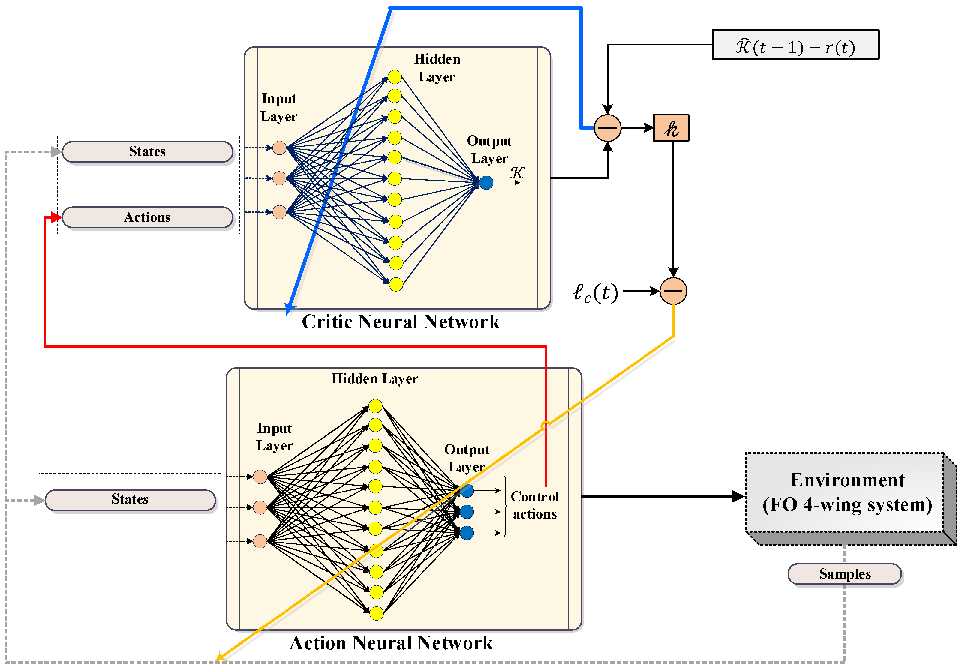
Adaptive dynamic programming (ADP) is one of the most prominent data-driven optimization algorithms, and is developed based on reinforcement learning (RL). In ADP, the optimal policy is achieved by the interaction between its agent with the environment. The ADP utilizes two distinct parts—policy iteration and value iteration—to reach the optimal policy. Two neural networks (NNs) are adopted in the structure of ADP—action NN and critic NN. The action NN aims to improve the performance of the system being studied by applying the optimal actions, while the quality of actions performed is evaluated by the critic NN. Moreover, a reward () is attributed to actions to guide the training procedure of the ADP agent.
In ADP, the cumulated discounted rewards should be enhanced during the training of NNs, which is given as:
where is the discount factor.
A Bellman’s equation is also utilized for estimating the long-term reinforcement (reward) signals. By utilizing this equation, recursive connection is created for the value function. According to Bellman’s equation, the main objective of ADP is expressed by [36]:
In the above equation, where is the optimal goal of the ADP at time t, x(t) denotes the state and the control action is indicated by the u(t).
The critic NN approximates the objective function through enhancing the reward signal. The error signal of the critic NN is calculated by the backpropagation scheme, which is defined by the following expressions:
By adopting the gradient descent, coefficients of the critic NN are updated by:
where and denote weights of input to hidden layers and output to hidden layers, respectively, belonging to the critic NN. ,…,, ,…,. In this equation, is the number neurons utilized in the hidden layer, is the number of neurons utilized in the input layer, and denotes the learning rate of the NN. and are the weights of input and hidden layers.
The primary updates of the action NN are realized by . The ultimate goals of action NN training are also realized by the backpropagation of error signals:
The backpropagation of the action NN is expressed as:
where and represent weights of input to hidden layers and output to hidden layers belonging to the action NN, respectively. ,…,, ,…,. Here, and are the number neurons utilized in the input layer and hidden layer, respectively, and is the learning rate of the action NN.
4.2. Design of Model-Free FTF-SMC Based on Dynamic Programming Learning
Since the system considered is highly chaotic, the design of controllers with parameters fails to control the system outputs. In this application, the training capability of the ADP agent is utilized to adaptively adjust the coefficients embedded in the model-free FTF-SMC control structure. States for the ADP training are considered:
According to the control law of (30), the set of tuning parameters play a critical role in the performance of the controller and should be adjusted by the ADP agent. During the interaction of the agent with the system, the optimal policy is obtained in such a way that minimizes the error signal.
For reaching fast response with small error, the reward function is defined as:
where and are positive weights.
The illustration of ADP for adaptive control of the FO 4-wing CS is depicted in Figure 3.
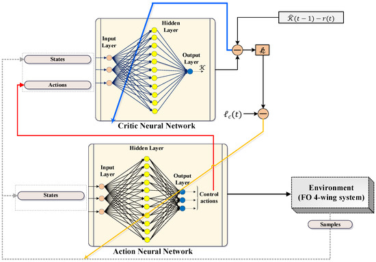
Figure 3.
Schematic of ADP with action and critic NNs for control of FO 4-wing CS.
Remark 3.
The ADP-optimized controller demonstrates superior performance compared to traditional model-based controllers by effectively handling model uncertainties, input constraints, and time delays without requiring precise system knowledge, leading to improved tracking accuracy and faster convergence. ADP was chosen over other reinforcement learning methods like DDPG or PPO primarily because it offers a more mathematically rigorous framework for stability and convergence guarantees in continuous-time control systems, particularly when combined with Lyapunov-based analysis. Additionally, ADP’s ability to incorporate cost function optimization directly within the control design process enables finite-time convergence and robustness, which can be more challenging to guarantee with general-purpose RL algorithms that often rely on trial-and-error and may require extensive tuning and data.
5. Simulation Results and Analysis
In this section, two distinct numerical scenarios involving the FO 4-wing CS (11) are explored to illustrate the effectiveness of the FTF-SMC approach. Furthermore, to demonstrate the enhanced performance of the FTF-SMC (30), the controller will be activated after 4 s. The numerical simulations were conducted using the high-order compact scheme algorithm outlined in references [51,52,53] with a time step of , implemented in MATLAB R2024b software.
5.1. Numerical Validation 1
Here, for , the FO 4-wing CS (11) demonstrates chaotic behavior, as indicated in [19]. The system’s initial conditions are given as , , , and . Additionally, the uncertainty terms of the system are considered:
, , , .
The parameters in SS dynamics (19) are set as for FTF-SMC (30), the parameters are defined as and for .5.
Moreover, the nonlinear control input ) is described as follows:
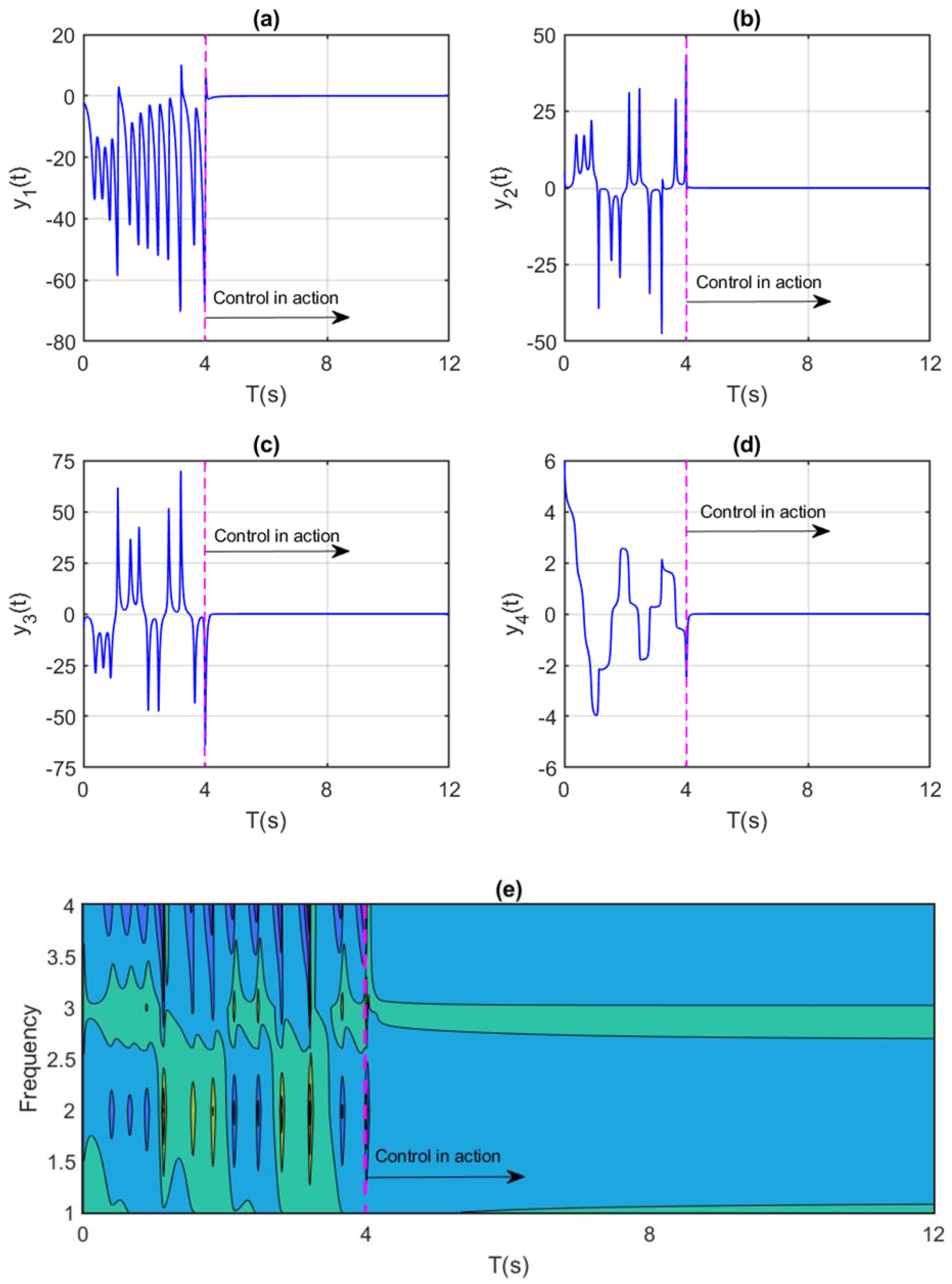
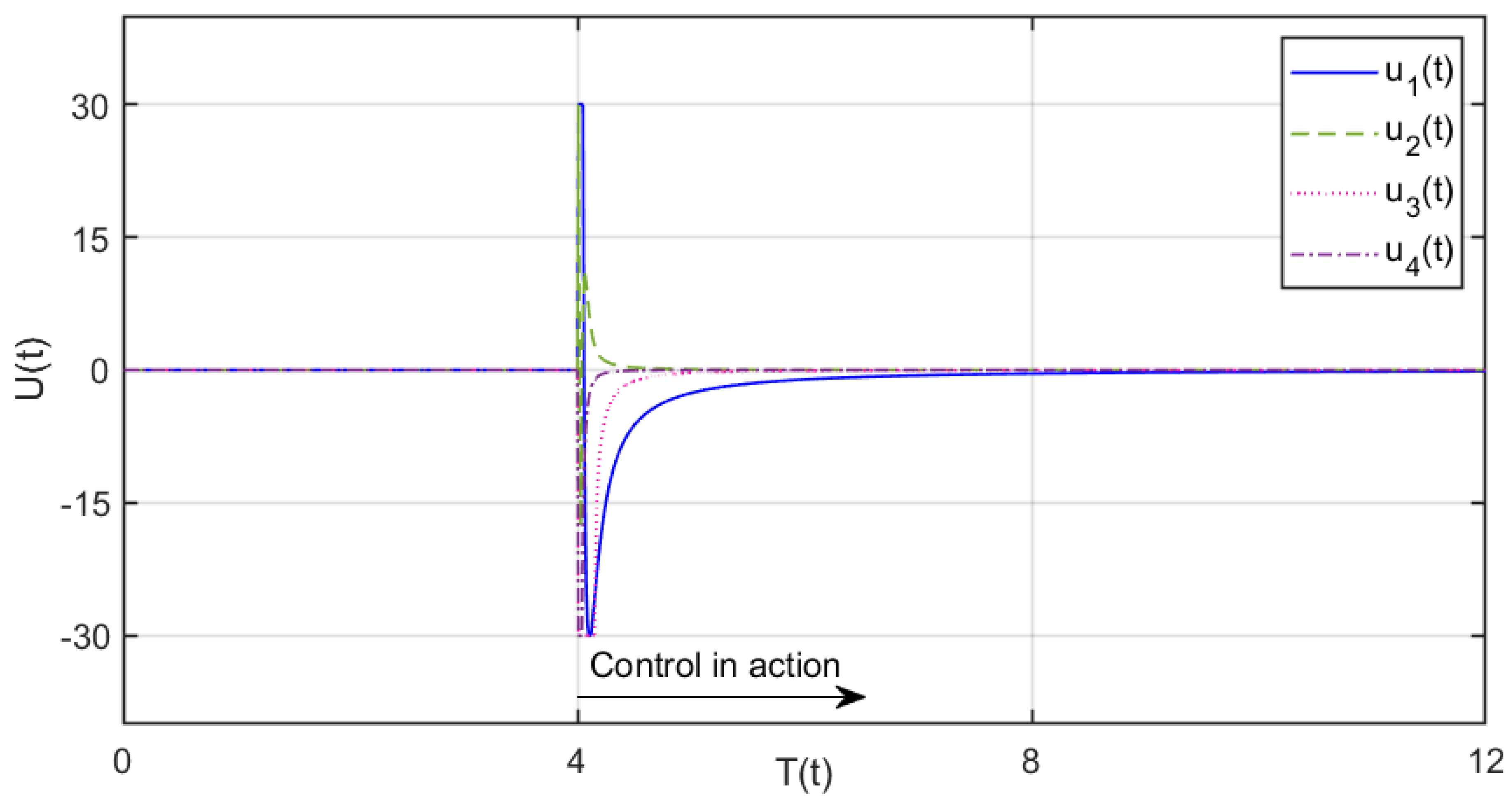
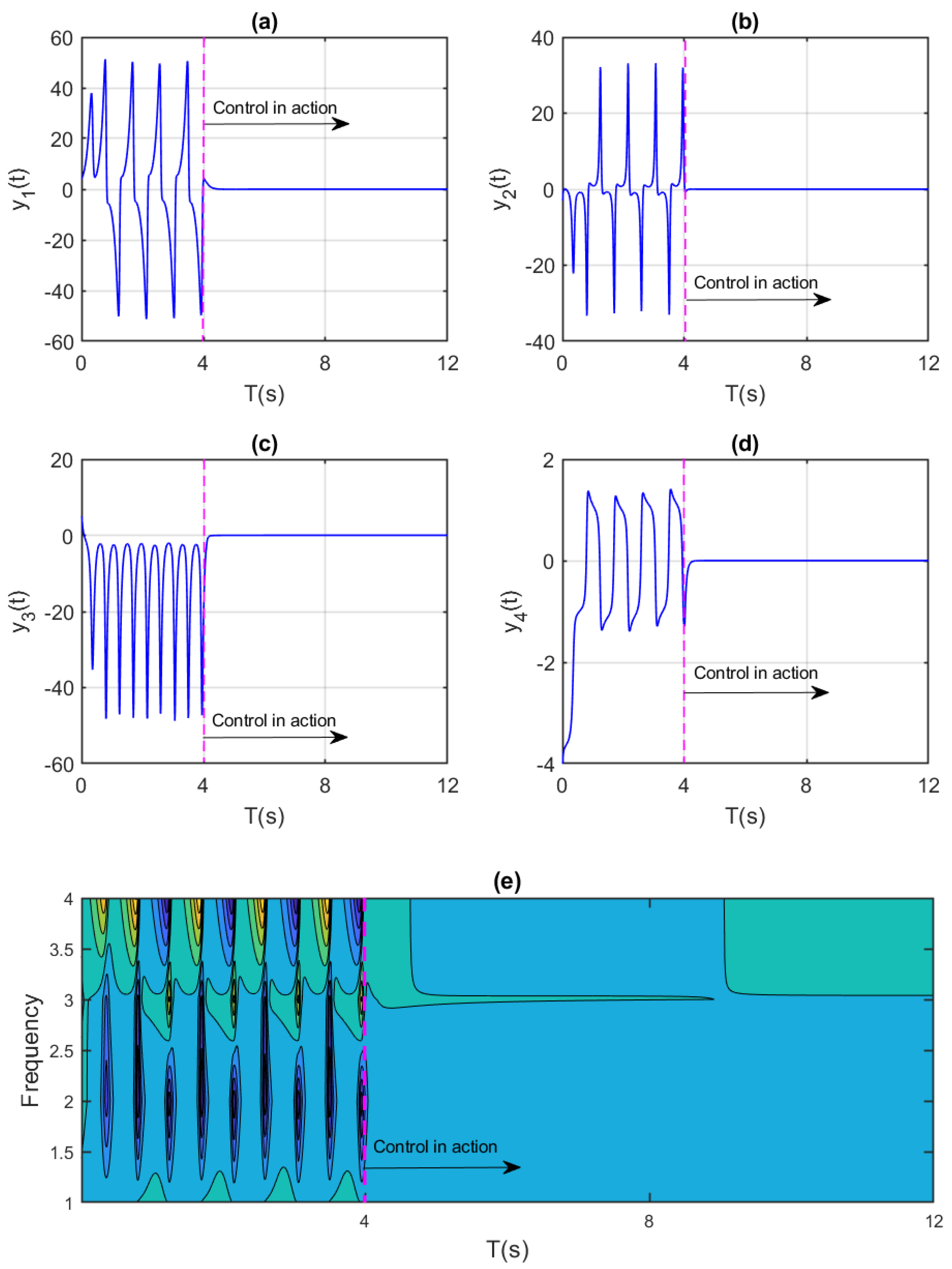
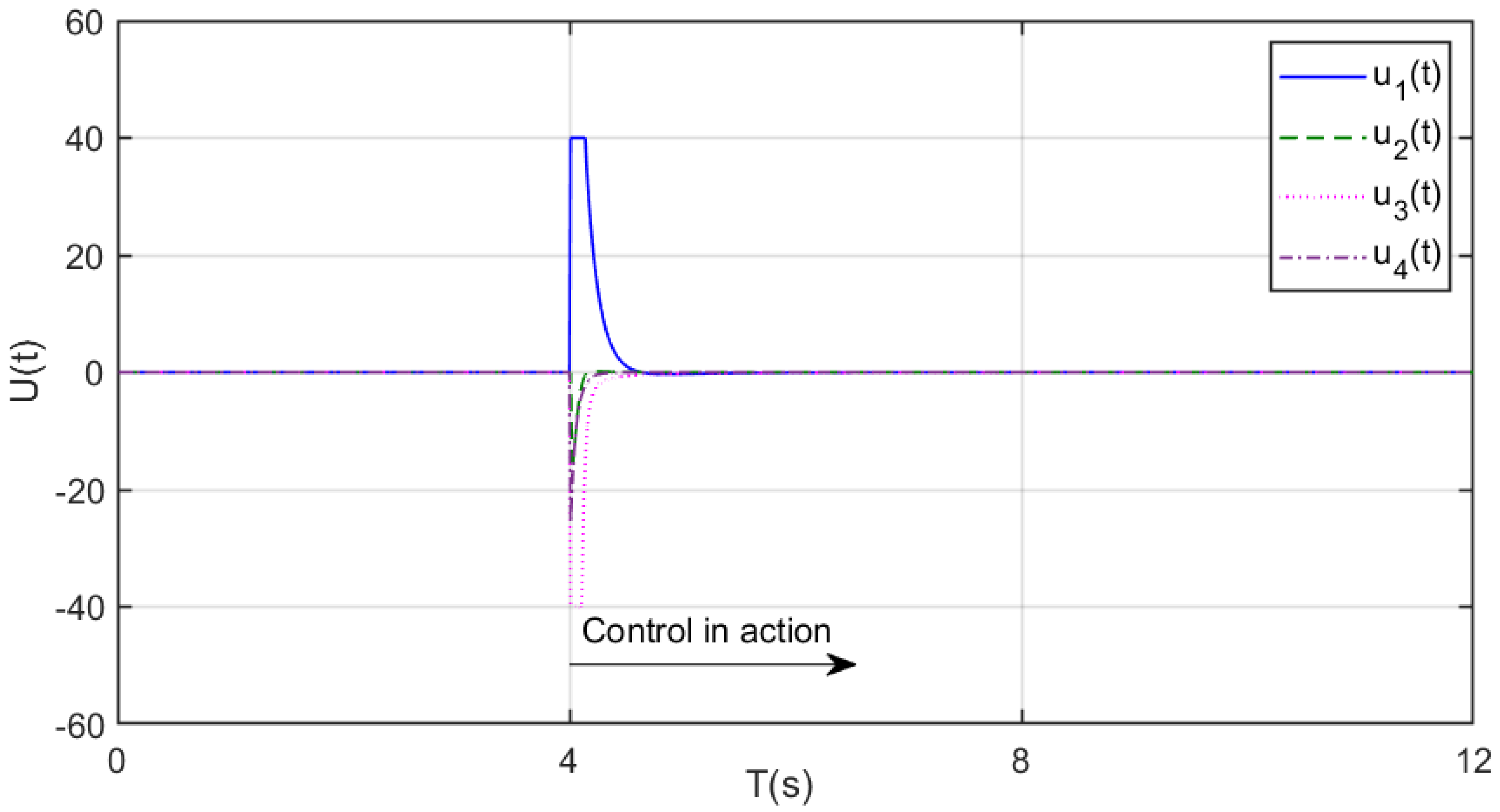
Figure 4a–d illustrate how states and in the chaotic FO 4-wing CS (11) are effectively stabilized using the FTF-SMC (30). Additionally, the pink line indicates that the controller operates at s. It is evident that all system states converge to the equilibrium point in finite time, demonstrating the effectiveness of the proposed control approach. Also, in Figure 4e, before control, the contour plot of an uncontrolled hyper-chaotic four-wing system is highly irregular, fragmented, and complex, exhibiting dense clusters and chaotic spread due to unpredictable dynamics. After operating the control method, the contours become smooth and structured as the system transitions from hyper-chaotic behavior to regular or periodic behavior, indicating stability. Furthermore, Figure 5 depicts the temporal dynamics of the FTF-SMC (30), demonstrating that the control input (52) steadily approaches equilibrium without exhibiting chattering effects. This finding emphasizes the capability of the developed adaptive controller to efficiently stabilize the four-dimensional chaotic FO 4-wing CS (11) in a finite time.
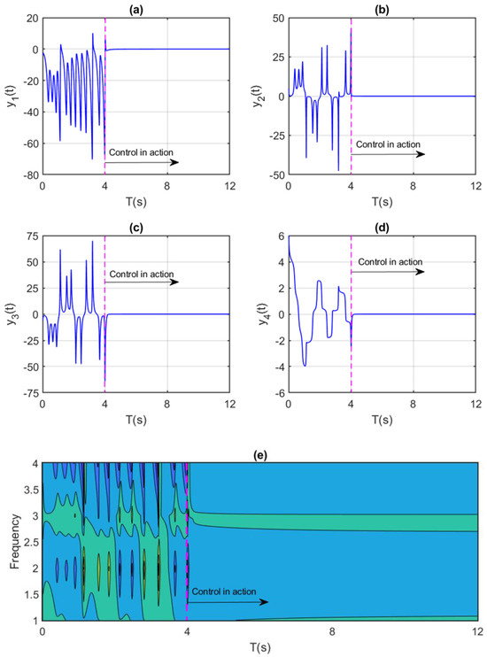
Figure 4.
Time history of the FO 4−wing CS (11) under the control of the FTF-SMC method (30) for . (a) the behavior of system state; (b) the behavior of system state; (c) the behavior of system state; (d) the behavior of system state; (e) the behavior of system states in contour plot view.
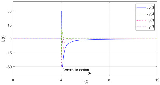
Figure 5.
Time-domain representation of the control input (30) applied to the FO 4−wing CS (11) for .
Additionally, as shown in Figure 5, when the control law signals (30) near the saturation boundary, the system triggers suppression due to the imposed saturation conditions. As a result, the occurrence of abrupt jumps is minimized. This characteristic ensures smoother transitions in jumping and switching states, which is particularly beneficial in scenarios involving relays and predefined saturation constraints.
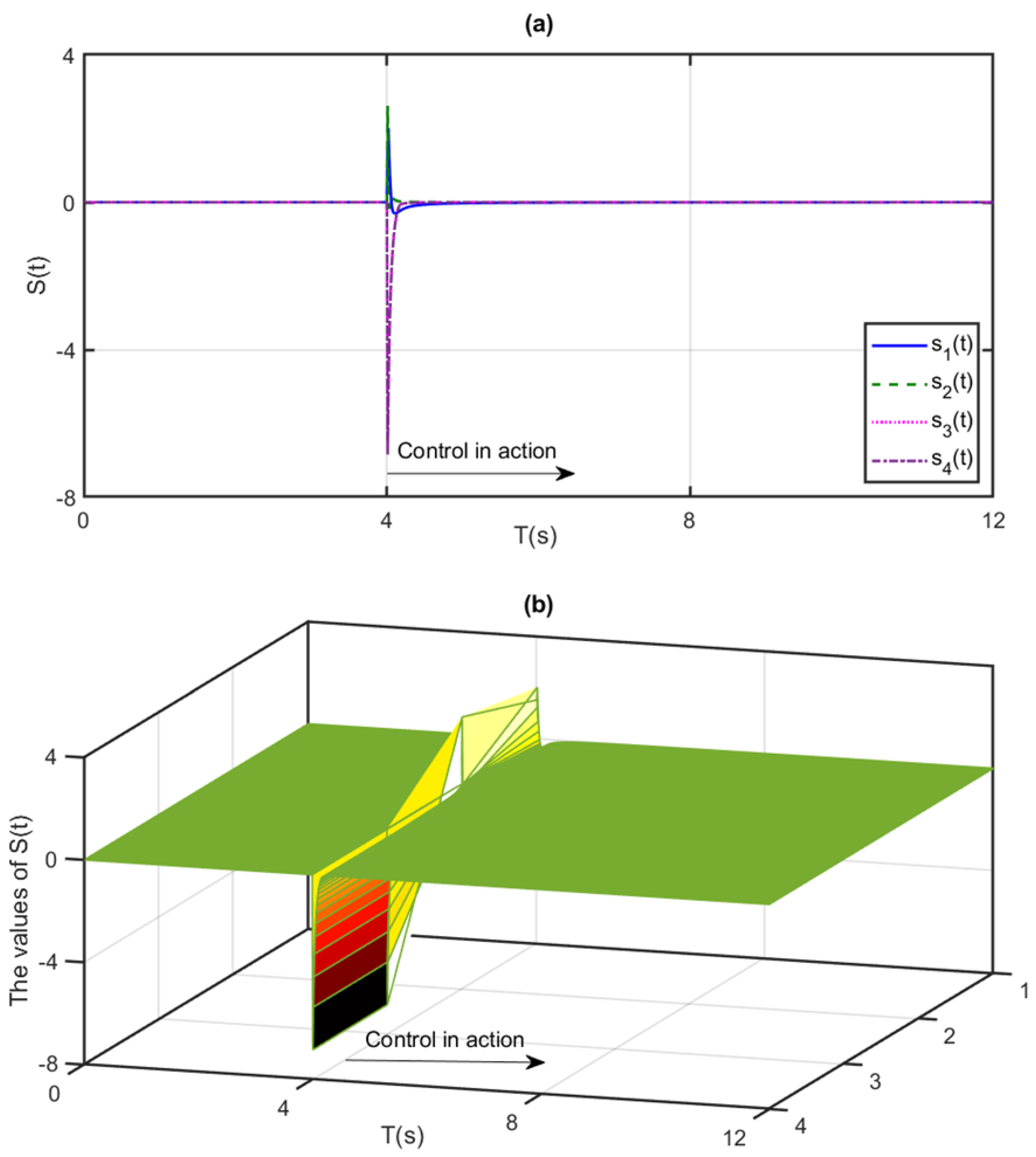
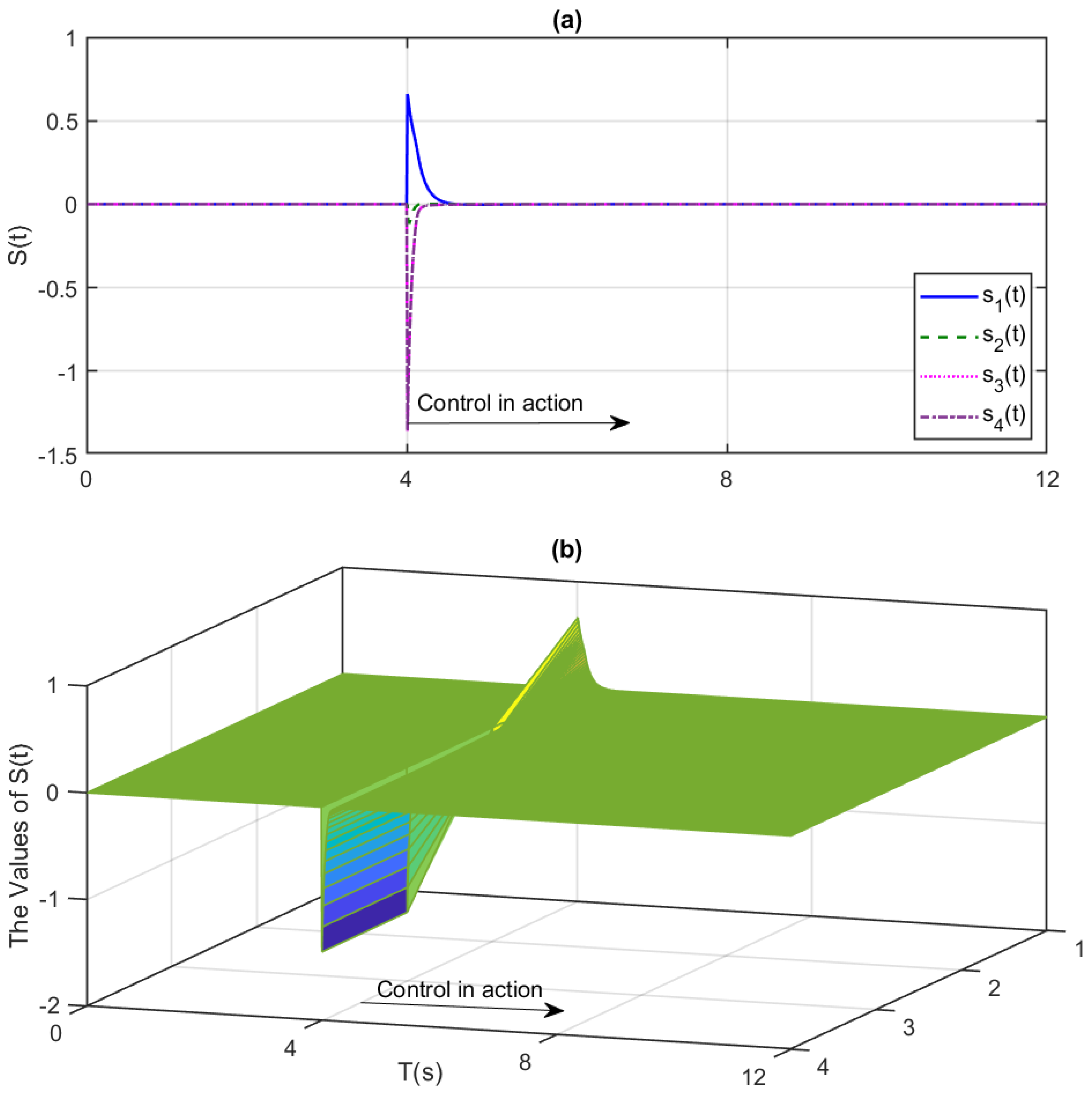
Moreover, Figure 6a,b illustrate the time response of the sliding surface (19) through a function plot and a surface plot, respectively. As evident in Figure 6a, each parameter of the sliding surface (19) converges to the origin, with no signs of chattering observed in the sliding surfaces. Additionally, Figure 6b confirms that implementing this approach results in a stable surface.

Figure 6.
Time-domain representation of the sliding surface (19) applied to the FO 4−wing CS (11) for : (a) 2-dimensional time-response of the sliding surface (19); (b) surface plot.
5.2. Numerical Validation 2
In this part, when the FO 4-wing CS (11) displays chaotic behavior, as stated in [19]. The system is initialized with the values , , , and . Furthermore, the uncertainty terms associated with the system are defined as follows:
, , , .
The parameters in SS dynamics (19) are fixed as for FTF-SMC (30), the parameters are defined as and for 5.
Moreover, the nonlinear control input is described as follows:
Figure 7a–d demonstrate the successful stabilization of the states and in the chaotic fractional-order (FO) four-wing system (11) using the FTF-SMC control method (30) for . Additionally, the pink line indicates that the controller operates at sec. The results clearly show that all system states reach the equilibrium point in finite time, highlighting the efficacy of the proposed control strategy. Additionally, Figure 7e reveals the chaotic nature of the uncontrolled hyper-chaotic four-wing system, characterized by irregular, fragmented, and complex contours with dense clusters and widespread chaotic behavior due to unpredictable dynamics. However, after applying the control method, the contours become smooth and organized, reflecting a transition from hyper-chaotic to regular or periodic behavior, which signifies system stability.
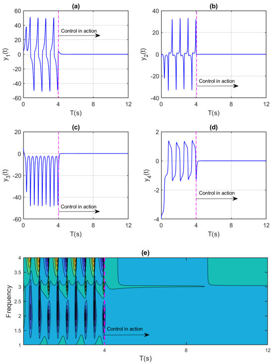
Figure 7.
Time history of the FO 4−wing CS (11) under the control of the FTF-SMC method (30) for . (a) the behavior of system state; (b) the behavior of system state; (c) the behavior of system state; (d) the behavior of system state; (e) the behavior of system states in contour plot view.
In Figure 8, the temporal dynamics of the FTF-SMC (30) are displayed, showing that the control input (53) smoothly approaches equilibrium without any chattering effects. This underscores the ability of the adaptive controller to effectively stabilize the four-dimensional chaotic FO 4-wing CS (11) within a finite time frame. Furthermore, Figure 8 also illustrates that when the control law signals (30) approach the saturation boundary, the system activates suppression mechanisms due to the imposed saturation constraints. This minimizes abrupt jumps and ensures smoother transitions during state switching, which is particularly advantageous in applications involving relays and predefined saturation limits.
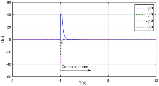
Figure 8.
Time-domain representation of the control input (30) applied to the FO 4−wing CS (11) for .
Moreover, Figure 9a,b present the time response of the sliding surface (19) through a function plot and a surface plot, respectively. Figure 9a indicates that all parameters of the sliding surface (19) converge to the origin without any chattering. Figure 9b further confirms that the implementation of this approach results in a stable sliding surface, reinforcing the robustness of the control method.
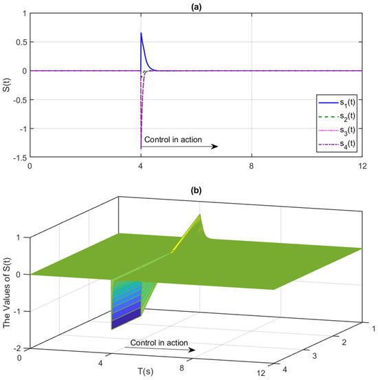
Figure 9.
Time-domain representation of the sliding surface (19) applied to the FO 4−wing CS (11) for : (a) 2-dimensional time response of the sliding surface (19); (b) surface plot.
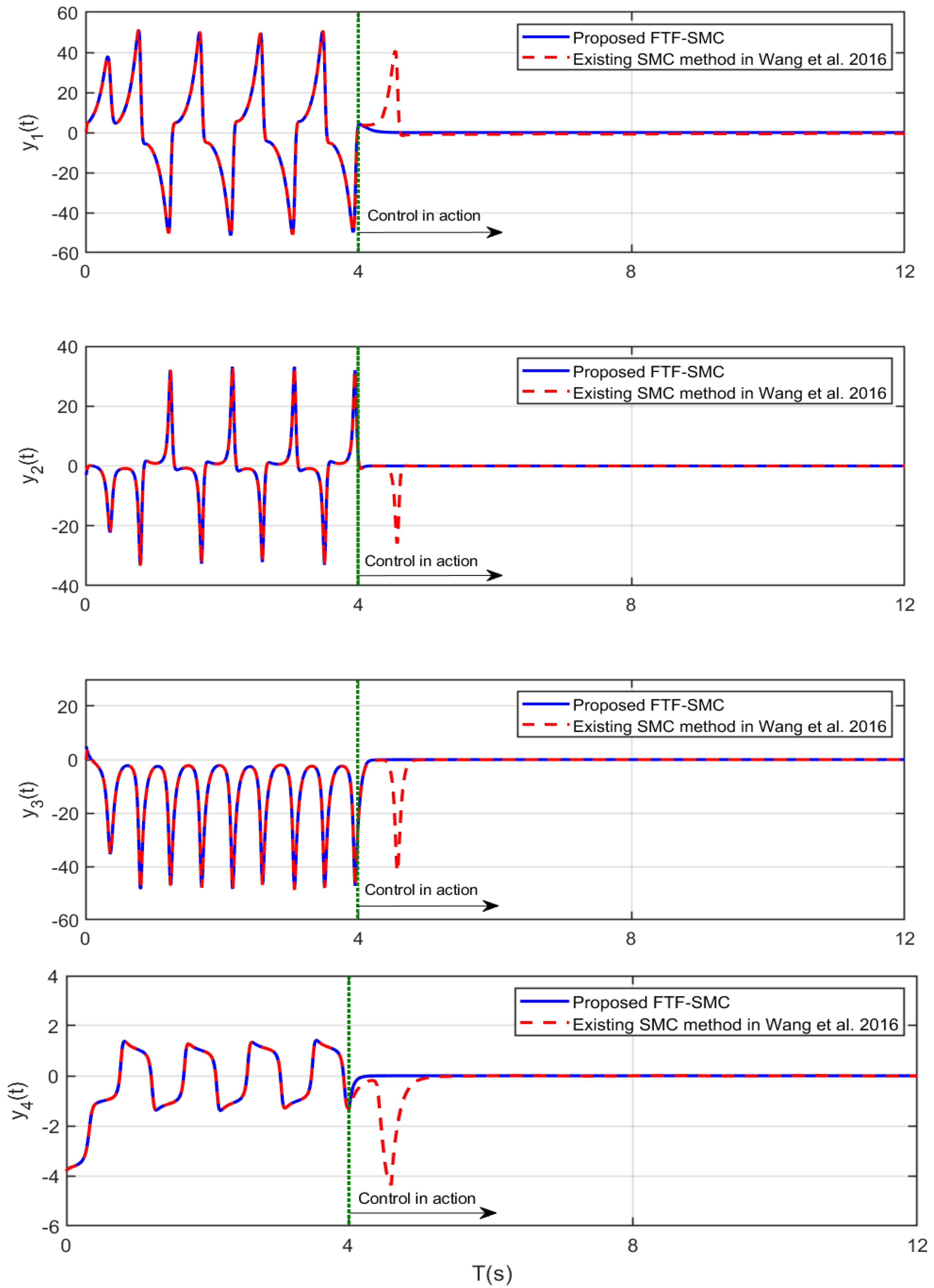
To provide a comparative analysis with the FTF-SMC (30), we also implement an alternative controller, as described in [54], for controlling the four-wing CS (11) defined by Equations (54) and (55) with . It is important to note that reference [54] addresses adaptive synchronization for a specific class of uncertain FO 4-wing CS (11) under external disturbances. In this study, for, , we apply the control strategy from [54] as follows:
Figure 10 presents the state trajectories of system (11) when controlled by the proposed FTF-SMC (30), as well as the SMC method (55) discussed in [54]. Additionally, the green line indicates that the controller operates at sec. Both control strategies successfully drive the system’s states to converge to the origin. However, a closer examination of the trajectories reveals that the proposed FTF-SMC achieves a more rapid and robust convergence compared to the traditional SMC method (55). This enhanced performance not only indicates a faster stabilization process but also suggests improved overall system behavior under the FTF-SMC strategy, making it a more effective solution for managing the dynamics of the system.

Figure 10.
Comparative analysis of state trajectories for the FO 4−wing CS under the proposed FTF−SMC (30) and the SMC method (55) introduced by Wang et al. [54].
Remark 4.
The reward function in the ADP framework (Equations (40) to (51) and Figure 10) is carefully designed to balance finite-time convergence and performance optimization by incorporating terms that penalize tracking errors and control efforts, ensuring that the system states rapidly approach the desired equilibrium while minimizing control energy. This design promotes a cost structure that inherently drives the policy toward stabilizing the system within a finite time horizon. During neural network training, stability is maintained by employing a Lyapunov-based analysis that guarantees the error signals between the estimated and true value functions remain bounded, alongside projection or normalization techniques that prevent parameter drift. Additionally, the learning rates and update laws are chosen conservatively to ensure monotonic improvement and avoid large oscillations. To prevent divergence or instability during policy updates, the algorithm uses a combination of critic–actor architectures with robust tuning of weight adaptation laws and often integrates smoothing or regularization terms to mitigate abrupt changes, thereby ensuring stable convergence throughout training.
Remark 5.
Despite the promising results, the proposed FTF-SMC framework has certain limitations that merit further investigation. One limitation lies in the computational burden associated with the online training of the ADP neural networks, which may pose challenges for real-time implementation, particularly on resource-constrained platforms. To address this, future research will focus on developing lightweight neural network structures and incorporating offline training or transfer learning strategies to reduce online computational load. Additionally, the current analysis assumes norm-bounded chaotic states to ensure finite-time stability, which may not hold for all classes of dynamical systems. As such, future work will aim to extend the control framework to accommodate unbounded or more irregular dynamics through adaptive bounding techniques or robust control formulations. Furthermore, experimental validation and deployment in real-world engineering applications, such as robotic systems or secure communication infrastructures, will be pursued to evaluate the practical viability and generalizability of the proposed approach.
Remark 6.
While the proposed FTF-SMC framework demonstrates strong theoretical and simulation-based performance, several important extensions remain for future investigation. Experimental validation on physical hardware platforms is a crucial next step to assess the controller’s robustness and effectiveness under real-world conditions, including sensor noise, actuator nonlinearities, and external disturbances. Additionally, broadening the scope of the framework to encompass other classes of chaotic systems, such as integer-order chaotic models and higher-dimensional systems, will further demonstrate its generalizability and practical relevance. To enhance real-time applicability, especially for resource-constrained embedded systems, future work will focus on improving the computational efficiency of the adaptive dynamic programming (ADP) training process. Techniques such as neural network pruning, model compression, and hybrid training algorithms will be explored to reduce computational load while maintaining control performance. These efforts aim to bridge the gap between theoretical control design and practical deployment, enabling robust and adaptive control solutions for a wide range of complex dynamical systems.
6. Conclusions
In this study, a novel model-free finite-time flexible sliding mode control (FTF-SMC) strategy was proposed to stabilize a specific class of hyperchaotic fractional-order four-wing (FO 4-wing) system under unknown uncertainties and input saturation constraints. FO 4-wing CSs are of great significance due to their complex dynamics and applications in secure communications, encryption, and nonlinear circuit design, making their stabilization a critical challenge. The proposed approach utilized fractional-order Lyapunov stability theory to design a flexible sliding mode controller capable of managing the chaotic behavior of FO 4-wing CSs and achieving finite-time convergence. A flexible dynamic sliding surface was introduced to adapt to system variations, followed by the development of a robust model-free control law to address uncertainties and input saturation. The finite-time stability of both the sliding surface and the control scheme was rigorously demonstrated. To enhance the parameters of the model-free FTF-SMC controller, a deep reinforcement learning approach leveraging the adaptive dynamic programming (ADP) algorithm is implemented. The ADP agent incorporates two neural networks (NNs)—the action NN and the critic NN—that work in tandem to optimize the policy by maximizing a specified reward function. Extensive simulations, numerical examples, and comparative analyses were conducted to validate the effectiveness of the proposed methodology. The results demonstrated that the MF-FTF-SMC approach not only effectively stabilized the FO 4-wing CS but also exhibited robustness against uncertainties and input saturation.
Author Contributions
Conceptualization, M.T.V. and V.H.P.; methodology, M.T.V., D.H.P. and H.L.N.N.T.; software, M.T.V., M.R. and S.H.K.; validation, M.T.V., M.R., S.H.K. and D.H.P.; formal analysis, H.L.N.N.T. and M.R.; investigation, V.H.P. and M.T.V.; resources, M.T.V., D.H.P. and M.R.; data curation, M.T.V. and M.R.; writing—original draft preparation, V.H.P., M.R. and M.T.V.; writing—review and editing, M.T.V. and V.H.P.; supervision, M.T.V.; project administration, V.H.P.; funding acquisition, V.H.P. All authors have read and agreed to the published version of the manuscript.
Funding
This research received no external funding.
Institutional Review Board Statement
Not applicable.
Informed Consent Statement
Not applicable.
Data Availability Statement
The original contributions presented in this study are included in the article. Further inquiries can be directed to the corresponding author(s).
Conflicts of Interest
The authors declare no conflicts of interest.
References
- Pham, D.H.; Vu, M.T. Takagi–Sugeno–Kang Fuzzy Neural Network for Nonlinear Chaotic Systems and Its Utilization in Secure Medical Image Encryption. Mathematics 2025, 13, 923. [Google Scholar] [CrossRef]
- Nguyen, V.T.; Pham, D.H.; Nguyen, Q.C.; Vu, M.T. Optimal design of Takagi-Sugeno-Kang fuzzy neural network based on balancing composite motion optimization for chaotic synchronization with uncertainty and disturbance. Results Eng. 2025, 25, 104234. [Google Scholar] [CrossRef]
- Li, D.; Tong, S.; Yang, H.; Hu, Q. Time-Synchronized Control for Spacecraft Reorientation With Time-Varying Constraints. IEEE/ASME Trans. Mechatron. 2025, 33, 2073–2083. [Google Scholar] [CrossRef]
- Wang, F.; Chen, K.; Zhen, S.; Chen, X.; Zheng, H.; Wang, Z. Prescribed Performance Adaptive Robust Control for Robotic Manipulators With Fuzzy Uncertainty. IEEE Trans. Fuzzy Syst. 2024, 32, 1318–1330. [Google Scholar] [CrossRef]
- Ji, L.; Lin, Z.; Zhang, C.; Yang, S.; Li, J.; Li, H. Data-Based Optimal Consensus Control for Multiagent Systems With Time Delays: Using Prioritized Experience Replay. IEEE Trans. Syst. Man Cybern. Syst. 2024, 54, 3244–3256. [Google Scholar] [CrossRef]
- Ju, X.; Jiang, Y.; Jing, L.; Liu, P. Quantized predefined-time control for heavy-lift launch vehicles under actuator faults and rate gyro malfunctions. ISA Trans. 2023, 138, 133–150. [Google Scholar] [CrossRef]
- Liang, J.; Yang, K.; Tan, C.; Wang, J.; Yin, G. Enhancing High-Speed Cruising Performance of Autonomous Vehicles Through Integrated Deep Reinforcement Learning Framework. IEEE Trans. Intell. Transp. Syst. 2025, 26, 835–848. [Google Scholar] [CrossRef]
- Hu, J.; Chen, B.; Ghosh, B.K. Formation–Circumnavigation Switching Control of Multiple ODIN Systems via Finite-Time Intermittent Control Strategies. IEEE Trans. Control Netw. Syst. 2024, 11, 1986–1997. [Google Scholar] [CrossRef]
- Holden, A.V. Chaos; Princeton University Press: Princeton, NJ, USA, 2014. [Google Scholar]
- Zhang, X.; Liu, Y.; Chen, X.; Li, Z.; Su, C. Adaptive Pseudoinverse Control for Constrained Hysteretic Nonlinear Systems and its Application on Dielectric Elastomer Actuator. IEEE/ASME Trans. Mechatron. 2023, 28, 2142–2154. [Google Scholar] [CrossRef]
- Meng, Q.; Ma, Q.; Shi, Y. Adaptive Fixed-Time Stabilization for a Class of Uncertain Nonlinear Systems. IEEE Trans. Autom. Control 2023, 68, 6929–6936. [Google Scholar] [CrossRef]
- En-Zeng, D.; Zai-Ping, C.; Zeng-Qiang, C.; Zhu-Zhi, Y. A novel four-wing chaotic attractor generated from a three-dimensional quadratic autonomous system. Chin. Phys. B 2009, 18, 2680. [Google Scholar] [CrossRef]
- Alikhanov, A.A.; Asl, M.S.; Huang, C.; Apekov, A.M. Temporal second-order difference schemes for the nonlinear time-fractional mixed sub-diffusion and diffusion-wave equation with delay. Phys. D Nonlinear Phenom. 2024, 464, 134194. [Google Scholar] [CrossRef]
- Roohi, M.; Aghababa, M.P.; Haghighi, A.R. Switching adaptive controllers to control fractional-order complex systems with unknown structure and input nonlinearities. Complexity 2015, 21, 211–223. [Google Scholar] [CrossRef]
- Alikhanov, A.A.; Asl, M.S.; Huang, C. Stability analysis of a second-order difference scheme for the time-fractional mixed sub-diffusion and diffusion-wave equation. Fract. Calc. Appl. Anal. 2024, 27, 102–123. [Google Scholar] [CrossRef]
- Li, C.; Su, K.; Zhang, J.; Wei, D. Robust control for fractional-order four-wing hyperchaotic system using LMI. Optik 2013, 124, 5807–5810. [Google Scholar] [CrossRef]
- Li, C.; Tang, Z.; Yu, S. A new 4D four-wing hyperchaotic smooth autonomous system and its improved form. In Proceedings of the 2011 Fourth International Workshop on Chaos-Fractals Theories and Applications, Washington, DC, USA, 19–22 October 2011; pp. 18–21. [Google Scholar]
- Zhang, R.-X.; Yang, S.-P. Modified adaptive controller for synchronization of incommensurate fractional-order chaotic systems. Chin. Phys. B 2012, 21, 030505. [Google Scholar] [CrossRef]
- Dadras, S.; Momeni, H.R.; Qi, G.; Wang, Z.-l. Four-wing hyperchaotic attractor generated from a new 4D system with one equilibrium and its fractional-order form. Nonlinear Dyn. 2012, 67, 1161–1173. [Google Scholar] [CrossRef]
- Li, X.; Li, Z.; Wen, Z. One-to-four-wing hyperchaotic fractional-order system and its circuit realization. Circuit World 2020, 46, 107–115. [Google Scholar] [CrossRef]
- Zhang, L.; Sun, K.; He, S.; Wang, H.; Xu, Y. Solution and dynamics of a fractional-order 5-D hyperchaotic system with four wings. Eur. Phys. J. Plus 2017, 132, 31. [Google Scholar] [CrossRef]
- Li, D.; Dong, J. Fractional-Order Systems Optimal Control via Actor-Critic Reinforcement Learning and Its Validation for Chaotic MFET. IEEE Trans. Autom. Sci. Eng. 2025, 22, 1173–1182. [Google Scholar] [CrossRef]
- Roohi, M.; Mirzajani, S.; Haghighi, A.R.; Basse-O’Connor, A. Robust stabilization of fractional-order hybrid optical system using a single-input TS-fuzzy sliding mode control strategy with input nonlinearities. AIMS Math. 2024, 9, 25879–25907. [Google Scholar] [CrossRef]
- Roohi, M.; Mirzajani, S.; Basse-O’Connor, A. A no-chatter single-input finite-time PID sliding mode control technique for stabilization of a class of 4D chaotic fractional-order laser systems. Mathematics 2023, 11, 4463. [Google Scholar] [CrossRef]
- Mirzajani, S.; Aghababa, M.P.; Heydari, A. Adaptive T–S fuzzy control design for fractional-order systems with parametric uncertainty and input constraint. Fuzzy Sets Syst. 2019, 365, 22–39. [Google Scholar] [CrossRef]
- Wei, Y.; Sheng, D.; Chen, Y.; Wang, Y. Fractional order chattering-free robust adaptive backstepping control technique. Nonlinear Dyn. 2019, 95, 2383–2394. [Google Scholar] [CrossRef]
- Tajrishi, M.A.Z.; Kalat, A.A. Fast finite time fractional-order robust-adaptive sliding mode control of nonlinear systems with unknown dynamics. J. Comput. Appl. Math. 2024, 438, 115554. [Google Scholar] [CrossRef]
- Hu, K.; Ma, Z.; Zou, S.; Li, J.; Ding, H. Impedance Sliding-Mode Control Based on Stiffness Scheduling for Rehabilitation Robot Systems. Cyborg Bionic Syst. 2024, 5, 99. [Google Scholar] [CrossRef]
- Li, X.; Rao, R.; Zhong, S.; Yang, X.; Li, H.; Zhang, Y. Impulsive control and synchronization for fractional-order hyper-chaotic financial system. Mathematics 2022, 10, 2737. [Google Scholar] [CrossRef]
- Oshnoei, S.; Aghamohammadi, M.R.; Khooban, M.-H. Model-free predictive frequency control under sensor and actuator FDI attacks. IEEE Trans. Circuits Syst. II Express Briefs 2023, 71, 2434–2438. [Google Scholar] [CrossRef]
- Lv, J.; Ju, X.; Wang, C. Neural network prescribed-time observer-based output-feedback control for uncertain pure-feedback nonlinear systems. Expert Syst. Appl. 2025, 264, 125813. [Google Scholar] [CrossRef]
- Zou, Z.; Yang, S.; Zhao, L. Dual-loop control and state prediction analysis of QUAV trajectory tracking based on biological swarm intelligent optimization algorithm. Sci. Rep. 2024, 14, 19091. [Google Scholar] [CrossRef]
- Mathiyalagan, K.; Sangeetha, G. Second-order sliding mode control for nonlinear fractional-order systems. Appl. Math. Comput. 2020, 383, 125264. [Google Scholar] [CrossRef]
- Dou, B.; Yue, X. Fractional-Order Sliding Mode Control for Free-Floating Space Manipulator With Disturbance and Input Saturation. Int. J. Robust Nonlinear Control 2025, 35, 3094–3115. [Google Scholar] [CrossRef]
- Chen, L.; Wu, R.; He, Y.; Chai, Y. Adaptive sliding-mode control for fractional-order uncertain linear systems with nonlinear disturbances. Nonlinear Dyn. 2015, 80, 51–58. [Google Scholar] [CrossRef]
- Saif, A.W.A.; Gaufan, K.B.; El-Ferik, S.; Al-Dhaifallah, M. Fractional Order Sliding Mode Control of Quadrotor Based on Fractional Order Model. IEEE Access 2023, 11, 79823–79837. [Google Scholar] [CrossRef]
- Mahmoud, T.A.; El-Hossainy, M.; Abo-Zalam, B.; Shalaby, R. Fractional-order fuzzy sliding mode control of uncertain nonlinear MIMO systems using fractional-order reinforcement learning. Complex Intell. Syst. 2024, 10, 3057–3085. [Google Scholar] [CrossRef]
- Gokyildirim, A.; Calgan, H.; Demirtas, M. Fractional-Order sliding mode control of a 4D memristive chaotic system. J. Vib. Control 2024, 30, 1604–1620. [Google Scholar] [CrossRef]
- Baishya, C.; Premakumari, R.N.; Samei, M.E.; Naik, M.K. Chaos control of fractional order nonlinear Bloch equation by utilizing sliding mode controller. Chaos Solitons Fractals 2023, 174, 113773. [Google Scholar] [CrossRef]
- Feliu-Talegón, D.; Rafee Nekoo, S.; Tapia, R.; Acosta, J.Á.; Ollero, A. Practical fractional-order terminal sliding-mode control for a class of continuous-time nonlinear systems. Trans. Inst. Meas. Control 2025. [Google Scholar] [CrossRef]
- Wang, F.-X.; Cui, J.-Q.; Zhang, J.; Lu, Y.-F.; Liu, X.-G. Stabilization of fractional nonlinear systems with disturbances via sliding mode control. Int. J. Robust Nonlinear Control 2025, 35, 202–221. [Google Scholar] [CrossRef]
- Znidi, A.; Nouri, A.S. Discrete adaptive sliding mode control for uncertain fractional-order Hammerstein system. Trans. Inst. Meas. Control 2025. [Google Scholar] [CrossRef]
- Narayanan, G.; Ali, M.S.; Joo, Y.H.; Perumal, R.; Ahmad, B.; Alsulami, H. Robust Adaptive Fractional Sliding-Mode Controller Design for Mittag-Leffler Synchronization of Fractional-Order PMSG-Based Wind Turbine System. IEEE Trans. Syst. Man Cybern. Syst. 2023, 53, 7646–7655. [Google Scholar] [CrossRef]
- Roohi, M.; Mirzajani, S.; Haghighi, A.R.; Basse-O’Connor, A. Robust Design of Two-Level Non-Integer SMC Based on Deep Soft Actor-Critic for Synchronization of Chaotic Fractional Order Memristive Neural Networks. Fractal Fract. 2024, 8, 548. [Google Scholar] [CrossRef]
- Podlubny, I. Fractional Differential Equations: An Introduction to Fractional Derivatives, Fractional Differential Equations, to Methods of Their Solution and Some of Their Applications; Elsevier Science: Amsterdam, The Netherlands, 1998. [Google Scholar]
- Li, C.; Deng, W. Remarks on fractional derivatives. Appl. Math. Comput. 2007, 187, 777–784. [Google Scholar] [CrossRef]
- Li, Y.; Chen, Y.; Podlubny, I. Stability of fractional-order nonlinear dynamic systems: Lyapunov direct method and generalized Mittag–Leffler stability. Comput. Math. Appl. 2010, 59, 1810–1821. [Google Scholar] [CrossRef]
- Pan, W.; Li, T.; Sajid, M.; Ali, S.; Pu, L. Parameter identification and the finite-time combination–combination synchronization of fractional-order chaotic systems with different structures under multiple stochastic disturbances. Mathematics 2022, 10, 712. [Google Scholar] [CrossRef]
- Curran, P.; Chua, L. Absolute stability theory and the synchronization problem. Int. J. Bifurc. Chaos 1997, 7, 1375–1382. [Google Scholar] [CrossRef]
- Fradkov, A.L.; Evans, R.J. Control of chaos: Methods and applications in engineering. Annu. Rev. Control 2005, 29, 33–56. [Google Scholar] [CrossRef]
- Asl, M.S.; Javidi, M. Numerical evaluation of order six for fractional differential equations: Stability and convergency. Bull. Belg. Math. Soc. -Simon Stevin 2019, 26, 203–221. [Google Scholar] [CrossRef]
- Alikhanov, A.A.; Yadav, P.; Singh, V.K.; Asl, M.S. A high-order compact difference scheme for the multi-term time-fractional Sobolev-type convection-diffusion equation. Comput. Appl. Math. 2025, 44, 115. [Google Scholar] [CrossRef]
- Alikhanov, A.A.; Asl, M.S.; Li, D. A novel explicit fast numerical scheme for the Cauchy problem for integro-differential equations with a difference kernel and its application. Comput. Math. Appl. 2024, 175, 330–344. [Google Scholar] [CrossRef]
- Wang, B.; Ding, J.; Wu, F.; Zhu, D. Robust finite-time control of fractional-order nonlinear systems via frequency distributed model. Nonlinear Dyn. 2016, 85, 2133–2142. [Google Scholar] [CrossRef]

Disclaimer/Publisher’s Note: The statements, opinions and data contained in all publications are solely those of the individual author(s) and contributor(s) and not of MDPI and/or the editor(s). MDPI and/or the editor(s) disclaim responsibility for any injury to people or property resulting from any ideas, methods, instructions or products referred to in the content. |
© 2025 by the authors. Licensee MDPI, Basel, Switzerland. This article is an open access article distributed under the terms and conditions of the Creative Commons Attribution (CC BY) license (https://creativecommons.org/licenses/by/4.0/).