Abstract
Proton exchange membrane water electrolyzers (PEMWEs) are a promising technology for green hydrogen production. However, the adoption of PEMWE-based hydrogen production systems remains limited due to several challenges, including high material costs, limited performance and durability, and difficulties in scaling the technology. Computational modeling serves as a powerful tool to address these challenges by optimizing system design, improving material performance, and reducing overall costs, thereby accelerating the commercial rollout of PEMWE technology. Despite this, conventional models often oversimplify key components, such as porous transport and catalyst layers, by assuming constant porosity and neglecting the spatial heterogeneity found in real electrodes. This simplification can significantly impact the accuracy of performance predictions and the overall efficiency of electrolyzers. This study develops a mathematical framework for modeling variable porosity distributions—including constant, linearly graded, and stepwise profiles—and derives analytical expressions for permeability, effective diffusivity, and electrical conductivity. These functions are integrated into a three-dimensional multi-domain COMSOL simulation to assess their impact on electrochemical performance and transport behavior. The results reveal that although porosity variations have minimal effect on polarization at low voltages, they significantly influence internal pressure, species distribution, and gas evacuation at higher loads. A notable finding is that reversing stepwise porosity—placing high porosity near the membrane rather than the channel—can alleviate oxygen accumulation and improve current density. A multi-factor comparison highlights this reversed configuration as the most favorable among the tested strategies. The proposed modeling approach effectively connects porous media theory and system-level electrochemical analysis, offering a flexible platform for the future design of porous electrodes in PEMWE and other energy conversion systems.
Keywords:
porosity modeling; spatial functions; analytical transport models; PEM water electrolyzer; multi-domain simulation; parametric sensitivity analysis MSC:
35Q79; 76S05; 76M10; 65M60
1. Introduction
Porous media modeling has become essential in the mathematical analysis of multiphase electrochemical systems, such as proton exchange membrane water electrolyzers (PEMWEs). These devices, widely recognized for their efficiency and responsiveness, operate through complex interactions involving fluid flow, ion and electron conduction, and gas evolution across layered porous domains. One key structural property—porosity—governs a wide range of transport parameters—including permeability, effective diffusivity, and electrical conductivity—and thus plays a defining role in performance [1,2,3,4,5].
However, most existing models simplify porosity as a constant value, primarily to ease numerical implementation. While useful for baseline simulations [3], this assumption fails to capture the true transport dynamics and through-plane heterogeneity revealed by imaging studies and the high-resolution characterization of real devices [6,7].
To address this limitation, the present study develops a function-based modeling framework that incorporates three representative porosity distributions—constant, linearly graded, and stepwise layered—into both analytical formulations and full-domain numerical simulations. These profiles are implemented as spatial functions embedded in analytical expressions that govern key transport properties. The numerical model evaluates their impact on current density, polarization behavior, and internal pressure distribution.
Although the focus of this paper is primarily mathematical, it aligns with the broader push toward green hydrogen as a pathway to decarbonization. Hydrogen has emerged as a crucial energy carrier for hard-to-abate sectors such as transport and heavy industry [8]. According to Bains et al. [9], in the International Energy Agency’s Global Hydrogen Review 2023, over 1000 hydrogen-related projects are currently underway worldwide. In particular, green hydrogen—produced via water electrolysis powered by renewable sources—is positioned as a key enabler of grid stability and energy security [10,11], with government-backed initiatives like the REPowerEU Plan accelerating deployment [12].
Within the water electrolysis family, PEMWE technology is increasingly adopted due to its compact design, high operating current densities, and ability to deliver high-purity hydrogen without corrosive electrolytes [1,2,11]. These advantages stem from the use of a solid proton exchange membrane, which ensures proton conductivity and acts as a barrier to crossover [11]. Consequently, PEMWE systems have seen wide deployment in the industrial hydrogen, mobility, and storage sectors [4,13].
However, the mathematical optimization of PEMWE structures still lags, particularly in addressing the internal porous regions. The porous transport layers (PTLs) and catalyst layers (CLs) are known to exhibit heterogeneous architectures—ranging from isotropic to gradually varying to multilayer configurations—depending on fabrication techniques and operational conditions [4,14,15,16]. Studies have shown that engineered porosity gradients enhance water transport, mitigate concentration polarization, and improve the uniformity of current density distribution [14,15,16]. Nonetheless, most simulation studies rely on empirical tuning or idealized assumptions, without rigorous mathematical formulation of spatial heterogeneity [6,7].
To fill this modeling gap, this work introduces a geometry-informed analytical framework in which porosity functions are mathematically defined and integrated into transport equations via Kozeny–Carman [3] and Bruggeman relations [3,17]. The sensitivity of the system to porosity variations is then assessed using a multi-level parametric study, isolating the effects of each layer’s porosity on key performance outputs.
This study builds on prior modeling efforts in fuel cells and electrolyzers [3,18,19], while advancing the integration of spatial microstructural variation into predictive electrochemical modeling. The resulting approach is generalizable and supports future extensions, such as two-phase flow modeling [17], anisotropic transport formulations, and the integration of real-world porosity distributions derived from tomography or image processing.
2. Materials and Methods
2.1. Structural Overview of a Typical PEMWE
A schematic of a typical PEMWE is presented in Figure 1. While design details may vary across systems, most PEMWE cells share a similar layered structure centered around the membrane electrode assembly (MEA). At the core lies a solid proton exchange membrane, typically Nafion, which facilitates selective proton transport from the anode to the cathode while blocking electron and gas crossover. This membrane is coated on both sides with CLs, composed of nanoscale pores and often made from precious metals such as iridium oxide (anode) and platinum (cathode). Adjacent to the CLs are the PTLs, which possess microscale pore structures and are generally fabricated from sintered titanium. These layers support water delivery, gas removal, and efficient current collection. In some high-temperature or dry-operating scenarios, PTLs may be replaced by gas diffusion layers (GDLs). Surrounding the MEA are additional structural and functional components. Bipolar plates (BPs), containing engineered flow field channels, facilitate uniform distribution of water and collection of evolved gases. They also provide electrical connectivity and mechanical support. Gaskets, typically made of perfluoroelastomer, ensure sealing and electrical insulation but are not depicted in Figure 1 for clarity. Similarly, current collectors—usually stainless-steel components responsible for transferring electrons—are excluded from the illustration. This study focuses specifically on the porous domains that influence transport phenomena, namely the PTL and CL, along with the solid membrane and BPs. These four layers are retained in the simulation and analytical models, as they are the primary regions where porosity variation affects performance.
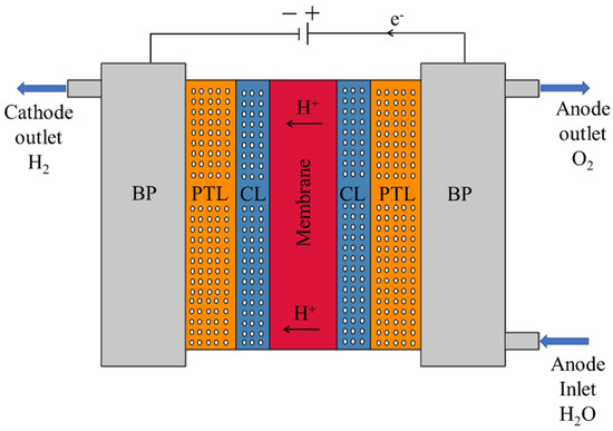
Figure 1.
Schematic representation of a typical PEMWE, showing the MEA and surrounding components. The MEA consists of a PEM (red), flanked by porous CLs and PTLs on both the anode and cathode sides. BPs house flow channels for water delivery and gas evacuation. Arrows indicate the direction of H+ transport and fluid flow.
2.2. Porosity-Dependent Transport Properties in PEMWEs
Porosity plays a pivotal role in defining the transport characteristics of porous layers in PEMWEs, particularly within the CL and PTL. Several effective properties—such as capillary pressure, permeability, diffusivity, and electrical conductivity—are strongly influenced by porosity, pore geometry, and their spatial distribution [3,4]. This section provides a detailed overview of the governing relationships between porosity and these transport properties, serving as a foundation for the analytical modeling introduced in the next section.
Porosity () is defined as the ratio of the pore volume (Vpore) to the total volume of the porous element (Vtotal) and can be expressed as
This fundamental relationship underpins the derivation of porosity-dependent parameters such as permeability, effective diffusivity, and electrical conductivity in the following subsections.
2.2.1. Permeability and the Role of Pore Size
Permeability () quantifies the ease with which a fluid can flow through a porous medium under a pressure gradient. In PEMWEs, it governs water and gas transport—especially in the PTL and CL—and is crucial for minimizing pressure drop, particularly at the anode, where liquid water enters and oxygen evolves [4,20]. A widely adopted semi-empirical correlation is the Kozeny–Carman equation, which relates permeability to porosity (), pore size (), and geometric structure of the pores:
This relation assumes randomly packed spheres but can be adapted for other geometries through specific surface area S and a correction factor C:
Here, is the specific surface area (pore surface area per unit volume), and is the Kozeny–Carman constant dependent on pore shape and tortuosity. To reflect more realistic pore morphologies in the PEMWE layers, Table 1 summarizes the characteristic values of S and C for spherical and cylindrical pores.

Table 1.
Specific surface area and Kozeny–Carman constants for typical pore geometries. The values of S and C are adapted from analytical pore models and prior parametric studies in fuel cell/electrolyzer literature [3,7].
In analytical derivations, the effective pore diameter is often related to the capillary radius from Equation (2) by . This relationship reinforces the nonlinear sensitivity of permeability to porosity—small variations in can result in large differences in , especially in dense structures like CLs.
In practice, the pore structures within the PEMWE components deviate from idealized geometries. While spherical and cylindrical pore assumptions aid analytical modeling, real porous media exhibit heterogeneous and anisotropic morphologies that vary across domains and even within layers. Factors such as fabrication technique, compression, and catalyst/ionomer distribution contribute to local variations in pore shape, tortuosity, and saturation [4,7,20]. As a result, the S and C values in Table 1 should be regarded as approximations. The Kozeny–Carman constant represents a geometric fitting factor dependent on pore morphology and tortuosity. While the classical value of C = 180 applies to packed spherical particles, lower values are often used for fibrous or cylindrical structures [3,7]. In this study, the selected C values in Table 1 ( for spherical and for cylindrical pores) are consistent with prior literature on electrochemical porous media and reflect common approximations for catalyst and transport layers in PEMWE simulations.
In typical PEMWE systems, PTLs are characterized by interconnected microscale pores ranging from 5 to 20 μm, often with spherical or irregular geometries, while CLs exhibit sub-micron pores between 10 to 500 nm, commonly cylindrical or mixed in shape [4,13]. These geometric distinctions directly influence the selection of pore diameter , Kozeny–Carman constant C, and surface area S in modeling. The accurate incorporation of these microstructural features enables more realistic permeability estimations, both in analytical formulations and numerical simulations. Their impact on transport resistance and flow behavior is evaluated in Section 3 through porosity-structured modeling.
2.2.2. Effective Diffusivity and Bruggeman Relations
Mass transport in porous domains, particularly gas diffusion through the PTL and CL, is commonly described using effective diffusivity (), which accounts for both the porosity and structural complexity of the medium. Due to the obstruction caused by the solid matrix and the tortuous pathways in porous media, the effective diffusivity is always lower than the bulk diffusivity of the fluid species.
A widely adopted relation to estimate the effective diffusivity is the Bruggeman relation, originally proposed for heterogeneous materials by Bruggeman in 1935 [17]:
In this expression, represents the effective diffusivity within the porous medium (m2/s), while is the diffusivity of the species in the bulk gas or liquid phase. The exponent , commonly referred to as the Bruggeman exponent, reflects the influence of the tortuosity and structural complexity of the porous network on diffusive transport.
Originally, Bruggeman derived this relation by analyzing the macroscopic behavior of mixtures of isotropic phases and proposed power law expressions for effective dielectric constants and conductivities in heterogeneous systems [17]. Over time, this formalism has been extended to model transport properties such as diffusivity and conductivity in porous media, assuming that the material behaves as a statistically homogeneous mixture.
In PEMWE-related systems, is often used as a baseline value, representing a simplified structure of randomly distributed and connected pores. However, Das et al. (2010) demonstrated that this assumption may significantly underpredict or overpredict transport behavior in CLs and gas diffusion media, depending on local pore morphology and degree of saturation [3]. To better capture these complex pore structures—including anisotropy and saturation effects—they introduced correction factors and modified transport equations, advancing the modeling framework “beyond Bruggeman.
While more advanced approaches—such as numerical pore-network modeling and LBM/CFD simulations—offer more accurate representation of microstructural effects, they are often computationally intensive and less amenable to parametric or optimization studies. In this work, we adopt the Bruggeman relation (with ) as a baseline model, not as the most accurate method, but as a widely accepted and analytically tractable approximation. This allows for isolating and examining the impact of porosity distribution strategies on mass transport behavior without introducing additional complexities associated with pore-scale simulations. The limitations of this assumption are acknowledged, and future work will explore more advanced modeling frameworks for the validation and extension of the proposed methodology. Numerous PEMWE modeling studies have employed the Bruggeman exponent β = 1.5 as a representative value for porous catalyst and transport layers, particularly under the assumption of isotropic pore structures [3,18,21]. This exponent is commonly treated as an empirical fitting parameter, reflecting the tortuosity and connectivity of the porous domain. While its exact value may range from 1.3 to 2.0, depending on the microstructure (e.g., fibrous versus granular media), using β = 1.5 provides a practical and widely accepted baseline. This choice balances physical realism and computational simplicity in single-phase transport models, enabling effective comparison across studies.
2.2.3. Electrical Conductivity in Porous Domains
In addition to mass transport, electrical conduction through both the solid and liquid phases in porous media is a key phenomenon governing PEMWE performance. The effective electrical conductivity () accounts for how porosity and microstructure influence charge transport pathways within the PTL and CL. Electronic conductivity occurs through the solid matrix (such as carbon, titanium, or metallic particles), while ionic conductivity takes place through the ionomer-filled pores or the liquid electrolyte.
Due to partial obstruction by the solid matrix and disconnection of pathways, the effective conductivity is always lower than the bulk conductivity of the conducting phase. A Bruggeman-type relation is often used to model this dependency:
Here, is the effective electrical conductivity, is the electrolyte volume fraction, and is the bulk conductivity (both in S/m). The Bruggeman approach, originally derived for isotropic composite materials [17], has become the foundation for transport modeling in porous electrodes.
However, as shown by Das et al. [10], this traditional relation may not accurately capture the conductivity behavior in realistic porous structures—especially in CLs—due to the influence of saturation, pore connectivity, and anisotropy. Their work introduced geometry-based correction factors to move beyond the Bruggeman approximation, improving the predictive accuracy of effective conductivity models in PEMWE systems.
Further studies using 3D simulations and experimental validation (e.g., by Jiang et al. [18] and Chen et al. [21]) confirmed that conductivity loss due to structural effects is non-trivial and spatially varying, particularly under dynamic operating conditions. This justifies the need to carefully represent porosity–conductivity relationships in both analytical and numerical models.
In this study, Equation (4) is used as a baseline to model porosity-dependent effective conductivity in both the CL and PTL under single-phase assumptions. Porosity profiles (constant, linear, graded) and their influence on local conductivity and overall performance are explored in Section 3.
2.2.4. Summary of Governing Transport Equations
The transport behavior in porous layers of PEMWEs is governed by a set of porosity-dependent relationships that define capillary pressure, permeability, diffusivity, and electrical conductivity. These properties are interrelated through the microstructure of the catalyst and transport layers, particularly their porosity and pore geometry. Table 2 provides a concise summary of the key transport equations used in this study. These relations serve as the foundation for the analytical modeling developed in Section 2.3 and the subsequent numerical simulations presented in Section 3. A Bruggeman exponent of was assumed throughout this study for all porous layers to calculate effective diffusivity and conductivity.
Table 2.
Governing transport equations and porosity dependencies.
2.2.5. Domain-Wise Pore Distribution and Layer-Specific Effects
In this study, pore size and porosity are treated as averaged values within each porous layer (PTL, CL, membrane, etc.) and are assumed to be uniform within each domain. This modeling approach does not account for intra-layer variations or node-level heterogeneity. It is therefore distinct from pore-scale or voxel-resolved methods that explicitly capture pore size distributions within a single layer, as discussed in related works [22,23].
Beyond pore size and shape, the spatial distribution of pores significantly influences fluid dynamics and electrochemical performance within PEMWE porous layers. Depending on the manufacturing process, pores may be evenly spaced, randomly arranged, or structured in specific patterns that enhance directional transport, pressure regulation, and gas removal.
In this study, six distinct pore distribution patterns are introduced—as shown in Table 3—each representing a different morphological strategy observed in real-world or engineered materials. These include uniform, random, graded, clustered, layered, and directional distributions, with qualitative descriptions of their structural features and potential effects on PEMWE performance.
Table 3.
Pore distribution types and their impact on PEMWE performance.
In PEMWEs, PTLs often exhibit random or graded pore distributions due to sintering and thermal processes during fabrication [4], while layered and directional structures are more common in advanced engineered materials such as coated foams, mesh layers, or printed multilayer CLs [13,24].
These distribution types are introduced here as theoretical design strategies found in the literature and materials science. However, they are not explicitly applied or analyzed in the simulations of this study. Future extensions of the present framework may incorporate spatial pore distribution models to explore their impact on transport resistance and electrochemical performance.
2.3. Analytical Modeling of Porosity Profiles
Understanding the influence of porosity on transport properties within the porous layers of PEMWEs is crucial for optimizing performance and minimizing losses. In this section, porosity is treated as a spatially varying function across the thickness of the PTL and the CL. Three types of porosity distributions are considered to investigate their impact on effective transport properties and electrochemical behavior: constant, linearly graded, and stepwise (multi-layer) porosity.
Each distribution reflects a different design or fabrication strategy. Constant porosity assumes a uniform microstructure, typical of conventional sintered titanium or carbon-based PTLs and CLs, and has been widely used in early models and experimental studies [1,4,7]. Recent work by Yuan et al. [4] further emphasizes the significance of microstructural uniformity in influencing liquid water pathways and gas bubble behavior. In contrast, linearly graded porosity mimics engineered structures in which porosity gradually changes along the thickness, tailored to enhance reactant penetration or product removal. This strategy has shown promise in advanced gas diffusion and transport layers [10,14,16]. Benmehel et al. [8] highlighted how graded PTL structures can improve through-plane water transport while mitigating saturation in specific zones. Lastly, stepwise porosity represents multi-layer architectures, where distinct porosity values are assigned to sub-layers. These configurations can be realized via layer-by-layer fabrication or partial sintering of coated substrates [13,24,25].
By incorporating these porosity variations into analytical expressions for permeability, effective diffusivity, and electrical conductivity—as outlined in Section 2.2.5—this framework enables a parametric evaluation of porosity effects under single-phase conditions. Section 2.3.1 introduces the general formulation of porosity profiles, and Section 2.3.2 applies them to representative PEMWE geometry. The resulting models serve as a mathematical foundation for exploring porosity-engineered designs, which are further validated through numerical simulations in Section 3. These porosity functions are illustrated schematically in Figure 2 to support the implementation described in Section 2.3.1.

Figure 2.
Schematic illustration of porosity profiles used in the simulations: (a) constant, (b) linear (e.g., rising or falling), and (c) stepwise. Profiles are applied along the through-plane (z) direction across the CL and PTL domains.
2.3.1. Generalized Porosity Profile Implementation
To capture spatial variation in the internal structure of porous media, porosity is treated as a continuous or piecewise-continuous function across the through-plane coordinate. This approach introduces a generalized porosity function, denoted by , where represents the distance through the thickness of a porous layer, and is the total thickness of that layer. Accordingly, defines the layer inlet and defines the outlet. The function can be embedded within analytical expressions for transport properties to assess the influence of engineered porosity on performance metrics. Three representative porosity profiles are considered in this work:
- Constant Porosity
This configuration assumes that the porosity remains uniform across the entire domain. It is often used in baseline models and represents conventional sintered materials with homogeneous structure.
- 2.
- Linearly Graded Porosity
A linear gradient is introduced along the z-direction, allowing porosity to gradually increase or decrease from the inlet to the outlet. This function supports the modeling of directional transport enhancement by tuning either reactant accessibility or product removal.
This formulation can represent either a rising or falling gradient depending on the relative values of and . represents the thickness of the porous layer.
- 3.
- Stepwise Porosity
In this piecewise profile, the layer is divided into two subdomains, each assigned a distinct porosity value. This configuration is commonly used to represent multilayer architectures fabricated via layer-by-layer coating, partial sintering, or graded material deposition. It reflects real-world designs where specific zones within a porous medium are tailored to support different transport requirements—such as facilitating reactant ingress in one region and enhancing product removal in another. The general form of the stepwise porosity function is expressed as
In this formulation, and represent the porosity values assigned to the two subdomains, while denotes the transition point at which the porosity value changes. The location of is not restricted to the midpoint; it may be defined arbitrarily depending on fabrication strategies, material characteristics, or performance optimization goals. The structure can be further extended to multiple subdomains by modifying the piecewise function accordingly.
These functional porosity profiles provide a flexible mathematical framework for embedding microstructural variation into transport property models. For example, permeability as a function of local porosity can be modeled using a Kozeny–Carman-type relation:
Similar formulations can be applied to effective diffusivity and electrical conductivity, allowing porosity-driven transport mechanisms to be explored under various design conditions.
While the next subsection applies these functions to a specific multi-layer PEMWE geometry, the mathematical formulation introduced here remains general and adaptable to any porous structure by redefining the spatial domain and porosity parameters.
2.3.2. Case-Specific Application: Layer Geometry and Volume Fractions
To demonstrate the implementation of the porosity profiles introduced in Section 2.3.1, this section introduces a representative PEMWE configuration consisting of seven layers: BP | PTL | CL | membrane | CL | PTL | BP. The structure is assumed to be symmetric about the membrane, and porosity functions are applied to the four porous layers: the two PTLs and two CLs. This configuration forms the basis for both the analytical calculations and numerical simulations discussed in Section 3.
- Geometrical Definition of Domains
The total cell height is denoted by , and the coordinate spans the full through-plane domain from the anode-side BP to the cathode-side BP. The membrane is treated as a non-porous solid region, while the PTLs and CLs are considered porous layers with potentially varying porosity. Let , , and denote the thicknesses of the membrane, each CL, and each PTL, respectively. The total modeled height of the domain can then be expressed as
- Volume Fraction Definitions
The volume fraction of each subdomain within the total cell is defined as
where
: fraction of the domain occupied by the membrane
: total fraction of the two CLs
total fraction of the two PTLs
These volume fractions are useful for calculating effective transport properties and scaling parameters and integrating porosity functions across the full domain. This formulation is consistent with established practices in the PEMWE modeling literature, where layer thicknesses are used to define volume fractions for analytical or numerical studies. For instance, similar methods are often applied to evaluate the impact of layer configurations on electrochemical and transport behavior.
- Design Relevance
This configuration reflects a common layer structure in PEMWE systems. By explicitly defining each layer’s thickness and location, the porosity functions from Section 2.3.1 can be assigned to the corresponding subdomains. For example, the anode-side PTL may use a rising linear profile, the CL may be modeled with either constant or falling porosity, and the cathode-side PTL may be treated using a stepwise function. These implementations will be evaluated numerically in Section 3 to study their influence on water distribution, gas transport, and cell performance under single-phase conditions.
2.3.3. Electrolyte Volume Fraction and Geometry-Based Domain Fractions
To support the analytical modeling of PEMWEs, this section introduces the concept of electrolyte volume fraction and defines the geometric contribution of each domain—membrane, CLs, and PTLs—based on their relative thicknesses. In most PEMWE configurations, the membrane is centrally positioned and coated on both sides with CLs and PTLs. For simplicity, each layer is assumed to be a cuboid with an identical length and width, allowing the total volume to be represented solely by layer thicknesses [1,4].
Let , , and denote the thicknesses of the membrane, CL, and PTL, respectively. The electrolyte volume fraction , defined as the ratio of the membrane thickness to the total domain height, is given by
Similarly, the volume fractions of the CLs and PTLs are expressed as
These fractions represent the proportion of each subdomain within the active region of the cell and obey the following condition:
It should be noted that these volume fractions are derived from a simplified 5-layer PEMWE geometry, consisting of the membrane, two CLs, and two PTLs. This formulation focuses solely on the electrochemically active region and does not include additional structural components such as bipolar plates. As a result, the calculated volume fractions may differ from those reported in broader simulation domains, such as Jiang et al. [18], where the domain setup encompasses more layers or inactive regions. The present formulation is designed to provide analytical consistency while isolating the structural role of ion-conducting and porous transport layers. This approach simplifies the integration of geometry into transport modeling. A higher indicates a dominant membrane phase, which may enhance proton conductivity but limit reactant/product accessibility. In contrast, higher PTL or CL fractions improve mass transport and gas evolution, but may increase ionic resistance if the membrane becomes too thin [1,11].
Typical PEMWE configurations feature membranes in the range of 50–200 μm, CLs between 5 and 50 μm, and PTLs from 100 to 500 μm. For example, a structure with 183 μm, 20 μm, and 500 μm yields 0.15, 0.03, and 0.82, highlighting the dominant role of porous domains in the overall structure [18].
These volume fractions are applied in the numerical model (Section 3) to assign porosity functions, define material domains, and evaluate the influence of geometrical variations on PEMWE performance.
2.4. Numerical Simulation Framework
Building on the analytical foundation developed in Section 2.2 and Section 2.3, this section presents a numerical modeling framework to evaluate how porosity distribution strategies affect PEMWE performance. A three-dimensional model is constructed based on a representative seven-layer geometry, incorporating porous domains (PTLs and CLs) with varying porosity profiles. The membrane is treated as a solid, ion-conducting phase, while the adjacent layers are simulated as porous media with tunable transport properties. Recent multiphysics modeling efforts, such as those by Østenstad et al. [26], demonstrate how integrated electrochemical, fluid, and thermal domains can enhance simulation fidelity in next-generation PEMWE systems. The objective is to compare constant, linearly graded, and stepwise porosity distributions across individual layers and assess their influence on key outputs such as current density and pressure distribution.
2.4.1. Modeling Strategy and Objectives
This study employs a three-dimensional numerical model to simulate a representative repeating unit of a PEMWE. The aim is to investigate the impact of porosity distribution strategies—specifically constant, linearly graded, and stepwise profiles—on transport and electrochemical performance within porous layers.
The model geometry includes seven layers arranged symmetrically:
BP|PTL|CL|membrane|CL|PTL|BP.
The membrane is treated as a non-porous, ion-conducting domain, while the PTLs and CLs are represented as porous media with user-defined porosity functions. These profiles are implemented in COMSOL Multiphysics 6.1 to control spatial variations in effective transport properties such as permeability, diffusivity, and electrical conductivity, based on empirical correlations introduced in Section 2.2 [1,10,20].
To isolate the effects of porosity alone, simulations are conducted under isothermal, steady-state, single-phase conditions—an approach widely used in PEMWE modeling to simplify the analysis of structural effects [1,21,25]. All cases share consistent boundary conditions, mesh configurations, and operating parameters, ensuring meaningful comparison between structural variants.
In the x-direction, symmetry boundary conditions (zero-flux Neumann) are applied to represent a repeating unit cell and minimize computational cost. While a 2D model in the zy-plane could simplify the simulation, we retained the full 3D domain to maintain compatibility with non-uniform porosity functions, allow future flow field coupling, and preserve potential in-plane transport variations.
This modeling framework enables the evaluation of the following:
- The influence of spatial porosity gradients on species distribution and current density
- The relative sensitivity of each porous layer to structural modifications
- The identification of porosity strategies that best balance transport efficiency and ohmic resistance
These insights support the rational design of next-generation PEMWEs by linking the structural tailoring of porous media to device-level performance optimization [4,18]
2.4.2. Geometry, Governing Equations, and Porosity Implementation
The numerical simulation is based on a representative three-dimensional repeating unit of a PEMWE, comprising seven layers arranged symmetrically as follows: BP | PTL | CL | membrane | CL | PTL | BP.
Each domain is modeled as a rectangular cuboid, and all layers share an identical width and length. This assumption simplifies the volume-based treatment of porous domains and isolates thickness () as the primary geometric variable influencing through-plane transport. The -direction is defined as the through-plane axis, with at the beginning of the anode-side BP and at the end of the cathode-side BP. Figure 3 presents the physical structure of the PEMWE cell used in this study. The top image illustrates the full 3D model, while the lower section provides a detailed cross-sectional view, highlighting the central membrane surrounded symmetrically by porous catalyst and transport layers. These domains serve as the primary focus for porosity-driven analysis of electrochemical and transport behavior.
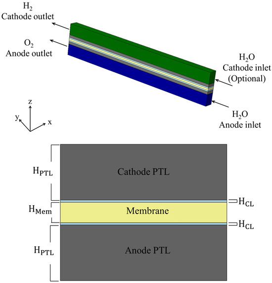
Figure 3.
Three-dimensional and cross-sectional visualization of the PEMWE model. The simulation domains include the membrane, CLs, and PTLs, bounded by impermeable BPs. All domains are treated as cuboids with identical a width and length.
The membrane is modeled as a non-porous, ion-conducting solid, while the adjacent CLs and PTLs are treated as porous domains. Porosity functions—constant, linear, or stepwise—are applied within these layers to assess their influence on cell performance. The BPs are assumed to be impermeable and electronically conductive.
This configuration provides a structured framework for assigning porosity profiles to individual domains. The porosity values in the PTLs and CLs are defined as either constant, linearly varying (rising or falling), or stepwise, based on the spatial coordinate system introduced in Section 2.3.1. Table 4 summarizes the thickness and z-direction allocation for each domain, along with the corresponding porosity function applied during the simulation.
Table 4.
Layer configuration, thickness, and -domain allocation for the PEMWE model.
In each porous region, porosity is expressed as a function of the normalized local coordinate , defined by
Here is the z-position at which layer begins, and is the thickness of the respective layer. This dimensionless coordinate facilitates the implementation of analytical porosity functions directly in the simulation environment and enables consistent application across domains of varying thickness.
2.5. Governing Equations and Modeling Approach
The simulation operates under steady-state, isothermal, and single-phase conditions. Although two-phase models are common in advanced PEMWE studies, a single-phase framework is adopted here for several justified reasons:
- Accuracy: Previous studies have shown that single-phase models can reliably capture transport and electrochemical trends, especially under moderate gas evolution [27,28,29,30].
- Clarity: This work’s primary goal is to isolate and evaluate the effect of porosity distributions. Two-phase models may introduce overlapping effects from gas–liquid interactions, obscuring porosity impacts.
- Efficiency: Single-phase models offer computational stability and reduced simulation time, enabling broad parametric studies.
The key governing equations are as follows:
- Mass Conservation in Porous Media:
- Momentum Conservation (Modified Navier–Stokes):
With the momentum, the source term due to the porous structure is given by
The flow field is modeled using a modified Navier–Stokes formulation, applied in a volume-averaged sense with porosity weighting and a Darcy resistance source term based on Kozeny–Carman permeability. Although the convective and viscous terms are often negligible in highly resistive domains, their inclusion allows for smooth coupling between adjacent porous and non-porous layers and enables future model extensions.
Here, is the dynamic viscosity, and is the permeability, calculated using Kozeny–Carman or other relations defined in Section 2.2. Finally, charge conservation and electrochemical kinetics are implemented to simulate the potential distribution and reaction activity within the porous domains. A full description of the potential computation and its coupling with electrochemical kinetics is provided in the ‘Electrochemical Transport’ subsection of this section.
- Electrochemical Transport
Electrochemical transport in the PEMWE cell is governed by Ohm’s law applied to porous domains, resulting in the following charge conservation equations for the protonic (membrane) and electronic (PTL + CL) phases:
Here, and are the electric potentials in the ion-conducting and electron-conducting phases, respectively (membrane vs. PTL + CL).
Note: In COMSOL’s built-in nomenclature, the membrane (proton-conducting) domain is referred to as the electrolyte phase, where the conductivity is denoted by , and the corresponding potential is . Similarly, the solid-phase (electron-conducting) materials are modeled under the electronic conducting phase, with conductivity and potential . These correspond to , and , in the present manuscript, respectively.
The effective conductivities and incorporate porosity correction via the Bruggeman relation (Equation (5)), i.e., , to account for tortuosity and reduced connectivity within the porous structures. The source terms and represent the interfacial current exchange and satisfy where is the local interfacial current density. The interfacial current density is evaluated using Butler–Volmer kinetics, adapted for PEMWE by incorporating electrode-specific parameters and a thermodynamic reversible voltage of 1.23 V, as given by
In this study, the anodic and cathodic transfer coefficients, denoted by and are treated as empirical constants, each set to 0.5, consistent with widely adopted assumptions in PEMWE modeling [18,29]. These values are commonly used to simplify charge transfer kinetics under symmetric electron–proton coupling conditions and have been employed in prior studies by Jiang et al. [18] and Toghyani et al. [29]. While experimental values may vary depending on the catalyst type and interface structure, assuming symmetry between anodic and cathodic transfer coefficients provides a reasonable approximation for comparing different porosity configurations. This approach also ensures consistency across kinetic expressions in single-phase electrochemical simulations. Here, is the exchange current density, is the Faraday constant, is the universal gas constant, is the operating temperature, and is the overpotential, defined as
The reversible cell potential is treated as constant and uniform in the single-phase model, consistent with prior work [3,17,29,31].
2.6. Boundary Conditions and Operating Parameters
To simulate electrochemical and transport processes within the PEMWE cell, realistic boundary conditions and operating parameters were applied, guided by experimental benchmarks and prior literature.
- Electrochemical Boundary Conditions
A cell voltage was applied between the two bipolar plates to drive the water electrolysis. The anode bipolar plate was assigned a constant potential of 1.23 V, while the cathode side was grounded at 0 V. This corresponds to the thermodynamic reversible voltage for water splitting under standard conditions (25 °C, 1 atm). However, in this study, the applied cell voltage varied between 1.2 V and 2.7 V across different simulation cases to evaluate porosity effects under a range of operating conditions. The full cell potential drop—capturing kinetic, ohmic, and mass transport losses—was computed based on the local current density and electrochemical kinetics in the CLs.
- 2.
- Flow and Pressure Boundary Conditions
Water was introduced through the anode inlet, and oxygen was removed at the anode outlet. The flow was treated as fully developed, incompressible, and laminar, consistent with single-phase operating assumptions. A constant outlet pressure of 1 atm was imposed on both the anode and cathode outlets, reflecting typical laboratory PEMWE setups. The inlet flow rate was set to 60 mL/min, in line with established benchmarks for single-phase simulations.
Although gas generation occurs during electrolysis, this model assumes a single-phase liquid flow to isolate the effects of porosity distributions on transport behavior and current generation.
While the present study adopts a single-phase liquid flow model to isolate and analyze porosity effects, it is important to acknowledge that two-phase transport—particularly involving gas generation and saturation phenomena—plays a significant role in practical PEMWE operation. Recent works by Guan et al. [32], Salihi and Ju [25], and Chen et al. [21] have demonstrated that multiphase flow modeling offers a more comprehensive representation of phase interactions, especially under high current densities. These approaches provide a valuable context for understanding transport bottlenecks and are recommended for future extensions of the current framework.
- 3.
- Material Properties and Layer Parameters
All material and geometric parameters were selected based on validated experimental data and simulation literature. Porosity values were implemented using constant, linear, or stepwise profiles, as described in Section 2.3. A complete summary of the operating and domain-specific parameters is presented in Table 5.
Table 5.
Operating conditions and simulation parameters used in the PEMWE model.
The values presented in Table 5 were selected based on the PEMWE cell configuration reported by Jiang et al. [18], which combines experimental measurements and simulation data. Specifically, a membrane thickness of 183 µm corresponds to the Nafion 117 membrane used in their experiments. The PTL and CL thicknesses (250 µm and 10 µm, respectively), as well as the operating pressure, flow rate, and conductivity values, were adopted directly from their validated setup. Additionally, this parameter set was employed in our previous PEMWE simulation study [30], which confirmed the accuracy of the model in reproducing polarization behavior and transport characteristics. This alignment ensures consistency with prior validated work and supports the credibility of the present analysis.
2.7. Meshing and Solver Settings
The numerical model was implemented in COMSOL Multiphysics 6.1 using a stationary study type. A tailored meshing strategy was applied to ensure high resolution in the porous domains—namely, the PTLs and CLs—where electrochemical reactions and transport resistances are most sensitive to structural variations. A structured hexahedral mesh was generated on the cross-sectional face and swept along the through-plane direction (z-axis) to maintain layer continuity and minimize skewness.
Finer mesh elements were concentrated within the CLs and at the membrane interfaces, capturing gradients in current density, overpotential, and pressure with greater accuracy. The membrane and non-porous domains were meshed with coarser elements to reduce computational load without compromising solution fidelity.
To solve the fully coupled system, a five-step solver sequence was developed to ensure convergence while gradually introducing complexity.
The numerical solution strategy followed a staged approach to ensure convergence and accurate initialization. First, a primary electrochemical initialization was performed by solving only the water electrolyzer physics and computing protonic and electronic potentials under ohmic losses alone, with activation and concentration effects excluded. This was followed by a secondary electrochemical solver step, which activated the full Butler–Volmer kinetics to incorporate both activation and concentration overpotentials within the CLs.
Next, an anode-side flow solver was applied to compute velocity and pressure fields in the anode PTL and CL using the Free and Porous Media Flow module under the assumption of single-phase, laminar flow. This was mirrored on the cathode side through a cathode-side flow solver, which applied the same flow physics to the cathode PTL and CL to properly initialize the complete flow field.
Finally, a fully coupled solution was carried out, solving all relevant physics—electrochemical and flow—in an integrated manner. A parametric sweep over the applied cell voltage was conducted during this step to generate polarization plots for different porosity configurations.
A relative tolerance of 10−3 was used across all solvers. Sequential initialization significantly improved stability and convergence speed, especially for simulations involving non-uniform porosity distributions. A representative image of the generated mesh is shown in Figure 4 to illustrate the structured meshing strategy applied across layers.

Figure 4.
Representative mesh used in the PEMWE simulation domain. The left panel shows the full 3D swept mesh across all domains, while the right panel presents a cross-sectional view highlighting local refinements near the catalyst layers and membrane interfaces.
2.7.1. Mesh Independence Test
A mesh sensitivity analysis was conducted to ensure that the numerical results were independent of mesh resolution. Three levels of grid refinement were considered: coarse, medium, and fine. The total number of elements varied from 1768 in the coarse mesh to 109,344 in the fine mesh, with the medium mesh consisting of 13,872 elements serving as the baseline case for comparison. Polarization plots obtained from these simulations showed negligible differences in the predicted current density between the medium and fine meshes. This observation is further supported by the quantitative values of maximum current density listed in Table 6, showing excellent agreement between the medium and fine meshes. As illustrated in Figure 5, the curves for the medium and fine meshes are nearly indistinguishable, confirming that further mesh refinement does not significantly affect the accuracy of the solution. Consequently, a medium-resolution mesh was adopted for all subsequent simulations to maintain a balance between computational efficiency and result fidelity.
Table 6.
Mesh refinement comparison.
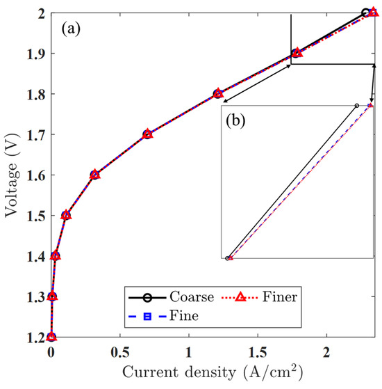
Figure 5.
Mesh resolution analysis: (a) polarization curves using three levels of mesh density, showing convergence in predicted performance, and (b) close-up view of the high-current-density region, confirming minimal deviation between the fine and medium meshes.
2.7.2. Convergence and Solver Stability
To ensure numerical stability and accuracy across the coupled physical domains, a staged solver strategy was implemented. In the first stage, the electrochemical module was solved independently, considering only ohmic losses to initialize the electric potential fields. The second stage activated the full Butler–Volmer kinetics, incorporating activation and concentration overpotentials within the CLs. Once the electrochemical response was established, the third and fourth stages sequentially solved the single-phase flow in the PTLs and CLs on the anode and cathode sides, respectively, using the Free and Porous Media Flow module. In the final stage, all governing equations and multiphysics couplings were fully activated and solved simultaneously using a stationary solver. A relative tolerance of 10−3 was consistently applied across all solver steps. To aid in convergence, a parametric continuation method was employed by introducing the cell voltage as a sweep variable, enabling gradual convergence toward the final operating condition. To complement the written solver description, Figure 6 presents a schematic overview of the numerical solution process.
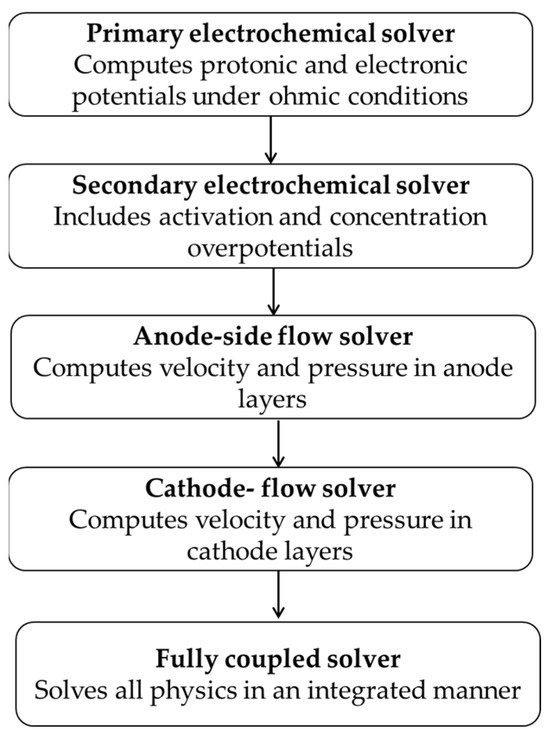
Figure 6.
Step-by-step numerical solving procedure used in the COMSOL simulation. The solver sequence begins with simplified electrochemical calculations and sequentially incorporates fluid flow in the anode and cathode before finally solving all coupled physics together.
To confirm the adequacy of the selected tolerance, a representative case was re-run with a tighter value of 10−4, which showed negligible change in the polarization curve. Additionally, residual monitoring confirmed that all physics modules converged below the 0.1% threshold across the simulations.
2.7.3. Validation and Model Limitations
To ensure the credibility of the model, a quantitative comparison was performed using polarization plots, as shown in Figure 7. The simulated polarization curve shows good agreement with both the experimental data reported by Ma et al. [35] and the two-phase numerical results presented by Jiang et al. [18]. This dual comparison validates the electrochemical formulation used in our model and confirms the consistency of the performance predictions under steady-state, single-phase conditions.
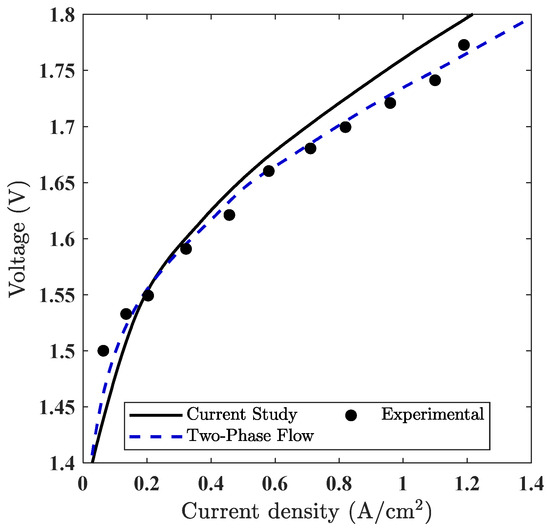
Figure 7.
Comparison of polarization curves obtained from the current PEMWE simulation (single-phase) with experimental data [35] and previously published two-phase simulation results by Jiang et al. [18].
To further quantify this agreement, a numerical error analysis was conducted using selected voltage–current data points extracted from the experimental study by Ma et al. [35]. The simulated polarization curve was interpolated at the same current densities, and error metrics such as absolute voltage deviation and percent error were calculated. The root mean square error (RMSE) was computed using the standard statistical formula across all matched points. These results are summarized in Table 7, which shows that the average percent error remains below 5%, and the RMSE is approximately 0.031 V. The data points used in Table 7 were extracted directly from the polarization curves shown in Figure 7, ensuring consistency in the comparison. This analysis confirms the predictive reliability of the model under the specified operating conditions.
Table 7.
Quantitative comparison between simulation and experimental polarization data, including absolute error and percent deviation at selected current densities.
However, direct experimental validation of spatial molar distributions of H2 and O2 within porous domains (PTLs and CLs) remains limited in the literature. This is primarily due to the difficulty of measuring species concentrations within operating electrolyzer structures. As a result, most available experimental studies focus on global performance metrics such as voltage–current relationships, rather than providing spatially resolved transport data.
In addition to the above validation, a qualitative trend comparison was also made with the earlier single-phase PEMWE model of Nie et al. [36]. While the geometry and operating conditions differ, our results show strong consistency in the influence of porosity on performance. This alignment in overall trends further supports the robustness of our modeling approach. A more detailed discussion of this comparison can be found in our recent review article, Bayat et al. [34], as well as in the original work by Nie et al. [36].
Several assumptions were made to simplify the computational domain and isolate the effects of porosity. The model considers steady-state, single-phase flow and neglects gas–liquid interactions, temperature gradients, and material heterogeneities. These idealizations clarify the interpretation of porosity-driven transport phenomena while reducing computational complexity. The staged solution approach—used to initialize and stabilize the coupled multiphysics system—is illustrated in Figure 7 and serves as a foundation for future model extensions involving two-phase transport, transient simulations, and direct integration with experimental diagnostics.
While the single-phase assumption enables a clearer interpretation of porosity effects, it may also overestimate transport performance, particularly at high voltages. In practical PEMWE operation, oxygen gas evolution in the anode-side porous domains can introduce two-phase flow effects—such as gas saturation, reduced permeability, and capillary resistance—that diminish the transport advantage of high porosity. For example, Guan et al. [32] developed a two-dimensional two-phase model incorporating charge transport equations of protons and electrons to examine the influence of PTL thickness on water distribution and cell performance. The results demonstrated that liquid saturation decreased from the channel to the CL, and the PTL had much lower liquid saturation, indicating that two-phase effects can significantly impact performance. In this work, we intentionally applied a simplified single-phase model as the first step to evaluate the impact of newly proposed porosity strategies under controlled conditions. Future work will build on this foundation to incorporate two-phase modeling and assess how porosity distributions behave under more realistic multiphase conditions.
Additionally, the present model assumes idealized, continuous porosity distributions in the CL and PTL layers. In reality, porous media often exhibit irregular and anisotropic structures that arise from manufacturing techniques and material agglomeration. High-resolution tomography studies have revealed complex pore geometries and heterogeneous networks that affect local transport behavior. Recent studies using high-resolution X-ray tomography have further highlighted the importance of porosity heterogeneity and multilayer architectures in PTL design, reinforcing the relevance of the porosity distributions analyzed in this study [37,38]. Future work can benefit from integrating experimentally derived porosity maps or stochastic geometry models to capture these microstructural effects more accurately.
2.7.4. Sensitivity Perspective on Two-Phase Effects
While the present study is based on single-phase assumptions to isolate porosity-related phenomena, it is important to acknowledge that under realistic operating conditions, two-phase flow can significantly alter transport dynamics—particularly within the PTL and CL. In saturated porous domains, the accumulation of gas bubbles reduces effective diffusivity and permeability by blocking liquid pathways. Conceptually, this can be captured by extending the Bruggeman relation to include a saturation penalty term, where the effective diffusivity is scaled not only by the porosity exponent , but also by a saturation factor such as , where is the local gas saturation and reflects increased resistance due to gas obstruction.
This insight, supported by prior two-phase modeling studies (e.g., Guan et al. [32], Salihi and Ju [25]), suggests that the transport benefits observed in high-porosity PTLs under single-phase assumptions may be significantly diminished—or even reversed—when gas saturation is high, particularly at elevated current densities.
A complete sensitivity analysis of saturation effects would require two-phase modeling with coupled transport properties that evolve with gas saturation, which is beyond the scope of this work. However, this conceptual framework serves to bridge the gap between single-phase modeling and more realistic multiphase dynamics. Future work will implement saturation-coupled transport formulations and explore their impact on PEMWE performance under dynamic operating conditions.
3. Results and Discussion
This section presents a detailed analysis of the numerical results obtained from the three-dimensional PEMWE model, with a focus on the effects of porosity distribution strategies on cell performance. The influence of various porosity distribution strategies—namely constant, linear, and stepwise—on key performance indicators, such as polarization behavior, pressure drop, species transport, and current density distribution, is systematically analyzed. In addition, a multi-level sensitivity analysis is conducted to evaluate the individual and combined effects of porosity variations across different porous layers. The results provide insight into how spatially tailored porosity profiles can enhance electrochemical performance and transport efficiency in PEMWEs.
While constant porosity is commonly assumed in PEMWE modeling for simplicity, it does not reflect the spatial heterogeneity observed in real PTLs and CLs. Experimental characterizations have revealed that porosity gradients often arise from fabrication methods such as sintering, spraying, or hot pressing, leading to inhomogeneous pore distributions [39,40,41]. Neglecting these gradients can underestimate transport resistance and misrepresent local current generation zones. Therefore, exploring linear and stepwise porosity profiles is essential to better represent structural variation and evaluate their influence on mass transport, water distribution, and overall cell performance.
3.1. Polarization Curve Comparisons
This section evaluates how constant porosity values across all porous layers influence polarization behavior in a single-phase PEMWE model. While the study also explores functionally graded porosity profiles (e.g., rising or falling linear, stepwise), the current comparison focuses on two reference cases, = 0.4 and = 0.8, each held constant throughout the anode PTL, anode CL, cathode CL, and cathode PTL.
Although higher porosity is generally associated with improved transport properties, the polarization curve results (Figure 8) reveal that this effect remains subtle under single-phase modeling conditions. Here, only water is modeled as a transport medium, and gas-phase transport mechanisms (oxygen/hydrogen evolution, capillary pressure) are not explicitly considered. As a result, porosity affects performance only indirectly—through the Bruggeman relation to effective diffusivity—with a limited impact at low to moderate voltages.
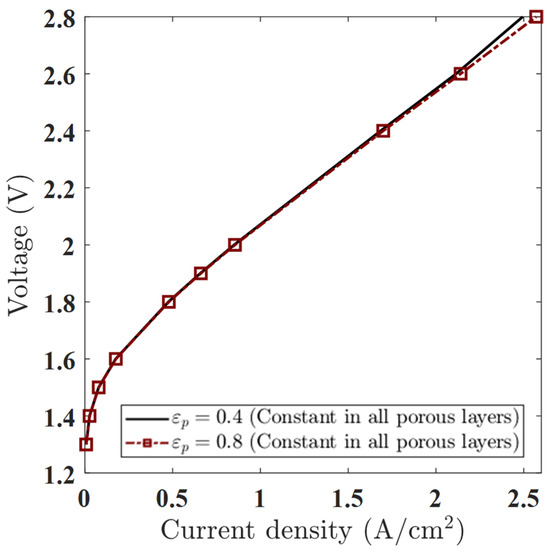
Figure 8.
Polarization curves for constant porosity values εₚ = 0.4 and εₚ = 0.8 in all porous layers, showing minor differences at low voltages and improved performance for εₚ = 0.8 at higher voltages.
Nevertheless, a voltage-dependent trend does emerge, with three distinct regimes:
- Low Voltages (1.3–1.6 V): Minimal Effect of Porosity
At low applied voltages, the polarization curves for εₚ = 0.4 and 0.8 are nearly indistinguishable. For example, at 1.5 V, the current density increases only marginally from 0.0783 A/cm2 (εₚ = 0.4) to 0.0789 A/cm2 (εₚ = 0.8). This negligible difference confirms that performance in this regime is dominated by electrochemical kinetics and ohmic losses, not by species transport. Since the model does not simulate gas accumulation or bubble-induced resistance, changes in porosity have minimal influence at these low current densities.
- 2.
- Moderate Voltages (1.8–2.0 V): Onset of Divergence
As the voltage increases to 1.8–2.0 V, a small but measurable divergence appears. At 2.0 V, the current density increases from 0.8500 A/cm2 (εₚ = 0.4) to 0.8550 A/cm2 (εₚ = 0.8). Although still minor, this suggests the beginning of transport-related performance enhancement. Increased porosity improves the effective diffusivity of water and dissolved gases, indirectly lowering species transport resistance, even in the absence of a modeled gas phase.
- 3.
- High Voltages (2.4–2.8 V): Clear Porosity-Driven Gain
At high operating voltages, the performance gap widens. At 2.8 V, the current density increases from 2.494 A/cm2 (εₚ = 0.4) to 2.571 A/cm2 (εₚ = 0.8)—a relative gain of ~3.1%. This indicates that even in a single-phase simulation, porosity can significantly influence mass transport behavior at high current densities, where concentration gradients and diffusion resistance become limiting. The higher εₚ reduces such gradients and facilitates the smoother evacuation of dissolved gases, setting the stage for larger improvements in future two-phase models.
3.2. Species Transport Behavior Under Varying Porosity Conditions
While the polarization curves demonstrated minimal changes across different porosity values under single-phase conditions, analyzing the spatial distribution of hydrogen and oxygen offers further insight into transport dynamics and internal species accumulation.
Figure 9 and Figure 10 present the molar fraction distributions of hydrogen and oxygen, respectively, for a porosity of 0.4 uniformly applied across all porous layers. Each figure contains six subfigures (a–f), corresponding to cell voltages ranging from 1.2 V to 2.7 V in 0.3 V increments. At low voltages (e.g., subfigures a–b), gas generation is modest and species are evenly distributed with minimal accumulation. As voltage increases (subfigures c–f), both hydrogen and oxygen concentrations rise significantly, with noticeable gradients forming toward the outlet due to limited diffusive removal. At 2.7 V, peak H2 and O2 molar fractions reach 0.875 and 0.940, respectively, reflecting strong transport limitations at high current densities.
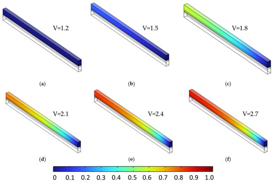
Figure 9.
Hydrogen molar fraction distribution in the cathodic porous region at a constant porosity of 0.4 across all layers, shown for increasing cell voltages from 1.2 V to 2.7 V in 0.3 V increments (subfigures (a–f)). As voltage increases, hydrogen generation intensifies, leading to progressive accumulation near the outlet due to limited diffusive transport in the single-phase model.
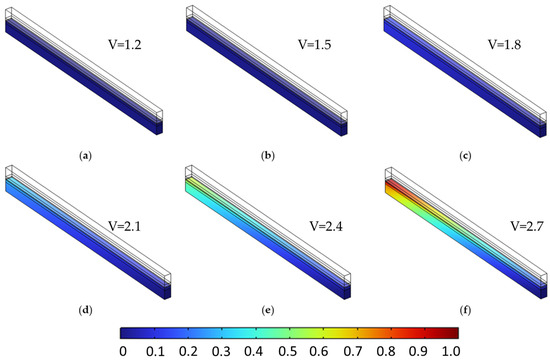
Figure 10.
Oxygen molar fraction distribution in the anodic porous region at a constant porosity of 0.4 across all layers, shown for cell voltages from 1.2 V to 2.7 V in 0.3 V increments (subfigures (a–f)). As voltage increases, oxygen generation intensifies, leading to greater accumulation near the outlet due to limited diffusion in the single-phase model.
Note: The observed accumulation of hydrogen and oxygen toward the outlet in Figure 9 and Figure 10 reflects the limitations of the single-phase modeling approach used in this study. In real PEMWE operation, gas bubbles typically migrate in the through-plane direction and are quickly released into adjacent flow channels due to capillary pressure gradients. As a result, such in-plane accumulation is unlikely under true two-phase conditions. This simplification, while useful for isolating the effect of porosity and voltage on dissolved species transport, will be addressed in future two-phase model extensions.
Figure 9 and Figure 10 provide the baseline species distributions at ε = 0.4, setting the stage for comparison. To investigate the role of porosity, Figure 11 and Figure 12 display the same voltage-dependent distributions for a higher porosity of 0.6. Compared to the lower-porosity case, species accumulation is visibly reduced at higher voltages. For instance, at 2.7 V (subfigure f), the peak hydrogen concentration decreases slightly to 0.872, and oxygen to 0.876. These reductions are attributed to enhanced effective diffusivity ( which facilitates more uniform gas evacuation and mitigates localized build-up. This effect is subtle but consistent across the mid to high voltage range (subfigures c–f), where transport limitations begin to dominate.

Figure 11.
Hydrogen molar fraction distribution in the cathodic porous region at a constant porosity of 0.6 across all layers, shown for cell voltages from 1.2 V to 2.7 V in 0.3 V increments (subfigures (a–f)). Compared to lower porosity, hydrogen accumulation is reduced and more uniformly distributed, indicating enhanced gas transport due to increased effective diffusivity.
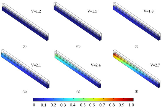
Figure 12.
Oxygen molar fraction distribution in the anodic porous region at a constant porosity of 0.6 across all layers, shown for cell voltages from 1.2 V to 2.7 V in 0.3 V increments (subfigures (a–f)). Higher porosity leads to reduced oxygen buildup and improved spatial uniformity, reflecting enhanced mass transport under increased diffusivity conditions.
This effect is also apparent when comparing the subfigures at 2.4 V (f) in Figure 9, Figure 10, Figure 11 and Figure 12, where the higher porosity cases exhibit smoother species profiles and lower peak accumulation, indicating more effective transport. To support these spatial observations, Table 8 compiles the peak H2 and O2 values at each voltage for both porosity cases, illustrating the consistent reduction in gas accumulation at = 0.6.
Table 8.
Maximum molar fraction values of hydrogen and oxygen at different voltages for two porosity cases ( = 0.4 and = 0.6). Higher porosity leads to slightly lower peak accumulation due to improved diffusivity, especially at higher voltages.
Overall, these results reinforce the value of porosity engineering for enhancing species transport within PEMWE porous layers. Even under single-phase assumptions, porosity influences gas distribution efficiency, especially at high operating voltages. This highlights the importance of internal diagnostics in complementing standard performance curves and lays the foundation for future two-phase modeling with capillary pressure and saturation effects.
These results are consistent with prior two-phase studies [18,25], which also reported that increasing porosity leads to improved gas removal and reduced species accumulation—particularly at high current densities where transport becomes limiting.
While the overall trends for uniform porosity confirm the expected role of effective diffusivity, they raise the question: Can non-uniform, layer-specific porosity profiles exert an even stronger influence on gas behavior and performance?
3.3. Effect of Stepwise Porosity in the Anode PTL on Species Distribution and Cell Voltage
To investigate the effect of non-uniform porosity in a single layer, this study applies a directionally engineered stepwise porosity profile to the anode PTL, transitioning from = 0.1 near the flow channel to = 0.7 near the membrane. While previous simulations used a constant porosity of = 0.4 throughout all porous domains, the modified configuration isolates the impact of porosity gradients on the anode PTL alone. The porosity of the anode CL, cathode CL, and cathode PTL remained fixed at 0.4.
This setup tests whether a sharp porosity shift in a single layer can influence gas transport and electrochemical performance. As shown in the polarization curve (Figure 13), the stepwise profile outperforms the constant case in the low to moderate voltage range. Below 1.8 V, the stepwise case delivers a higher current density—e.g., at 1.6 V, the current increases from 0.401 A/cm2 (constant) to 0.425 A/cm2 (stepwise)—indicating improved water access and mass transport efficiency. However, at higher voltages (e.g., 2.4 V), the performance advantage diminishes, and the constant porosity case slightly outperforms the stepwise one. This reversal suggests increased local resistance or oxygen accumulation in the low-porosity zone near the channel.
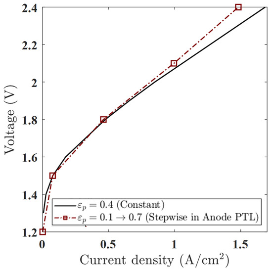
Figure 13.
Polarization curves for constant porosity (εₚ = 0.4) and stepwise porosity in the anode PTL (εₚ = 0.1 → 0.7, from channel to membrane). The stepwise case shows improved performance below 1.8 V due to enhanced water transport, but slightly higher overpotentials at high voltages due to increased oxygen accumulation and local resistance near the channel.
The species distribution plots (Figure 14 and Figure 15) further illustrate these effects. In particular, Figure 15 shows the increased oxygen accumulation near the channel in the stepwise case, resulting from the low-porosity region adjacent to the flow field. This creates a transport bottleneck that limits gas evacuation, despite the high-porosity region near the membrane that facilitates reactant access. Figure 14 also confirms a slightly more uniform hydrogen distribution in the stepwise case at elevated voltages, though the difference is less pronounced than for oxygen.
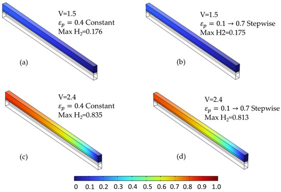
Figure 14.
Comparison of hydrogen molar fraction distribution at two voltages for different anode PTL porosity configurations. (a,c) Constant porosity (εₚ = 0.4) at 1.5 V and 2.4 V, respectively. (b,d) Stepwise porosity (εₚ = 0.1 → 0.7, from channel to membrane) at the same voltages. Minor differences are observed at 1.5 V, while more uniform hydrogen distribution occurs in the stepwise case at 2.4 V.

Figure 15.
Oxygen molar fraction distribution at selected voltages for two porosity configurations in the anode PTL. (a,c) Constant porosity (εₚ = 0.4) at 1.5 V and 2.4 V, respectively. (b,d) Stepwise porosity (εₚ = 0.1 → 0.7, with the low-ε zone near the channel) at the same voltages. The stepwise configuration results in significantly higher oxygen accumulation near the membrane—particularly at 2.4 V—due to hindered transport caused by the upstream low-porosity region.
To quantify these trends, the maximum molar fractions of hydrogen and oxygen were extracted at six voltage levels across all three configurations—constant porosity, stepwise (0.1 → 0.7), and reversed stepwise (0.7 → 0.1) profiles in the anode PTL. The stepwise case consistently resulted in higher peak oxygen concentrations, particularly in the mid to high voltage range. For instance, at 2.1 V, the O2 maximum increased from 0.311 to 0.620, a 99% rise. At 2.7 V, oxygen reached saturation in both cases, though the stepwise profile still showed a higher peak. In contrast, hydrogen concentrations remained similar or slightly lower in the stepwise case at higher voltages, likely due to elevated transport resistance and reduced current generation.
To further investigate the effect of porosity direction, a second simulation was conducted using a reversed stepwise profile, where εₚ transitions from 0.7 near the channel to 0.1 near the membrane. This adjustment aimed to alleviate the transport bottleneck near the reaction interface by increasing local permeability. The consolidated results are presented in Table 9, allowing direct performance comparison of hydrogen and oxygen accumulation across the three porosity strategies.
Table 9.
Maximum H2 and O2 molar fractions at different voltages for three anode PTL porosity profiles: constant (εₚ = 0.4), stepwise (0.1 → 0.7), and reversed stepwise (0.7 → 0.1). The reversed profile reduces oxygen accumulation at high voltages, while hydrogen transport remains largely unchanged.
To complement the species concentration results, we also analyzed the local electrode current density distribution within the anode PTL. Figure 16 presents 2D maps of the electronic current density under the three porosity configurations at 2.4 V, revealing subtle shifts in charge transport behavior due to the imposed porosity gradients.
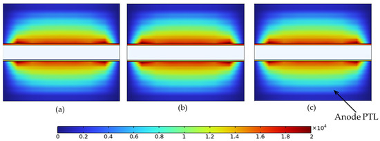
Figure 16.
Local electrode current density (A/m2) in the anode PTL at 2.4 V for (a) constant porosity (εₚ = 0.4), (b) stepwise porosity (εₚ = 0.1 near the channel → 0.7 near the membrane), and (c) reversed stepwise porosity (εₚ = 0.7 near the channel → 0.1 near the membrane). Maximum values are 1.96 × 10⁴, 1.75 × 10⁴, and 1.96 × 10⁴ A/m2 for (a), (b), and (c), respectively.
As shown in Figure 16, all three porosity configurations exhibit a similar overall current distribution pattern due to the dominant through-plane conduction path. However, subtle differences emerge in the peak values and current concentration. The stepwise profile (b), with low solid content near the channel, exhibits a slightly lower maximum current density (1.75 × 10⁴ A/m2), indicating weaker electronic conductivity in that region. In contrast, the constant (a) and reversed stepwise (c) profiles reach higher peaks of 1.96 × 10⁴ A/m2, enabled by greater solid connectivity near the channel. These results support the previous mass transport findings and demonstrate that porosity gradients in the PTL can influence charge transport, even in single-phase operation.
Although the 0.1 → 0.7 configuration increased cell voltage and promoted local O2 build-up, it clearly demonstrates the system’s sensitivity to porosity distribution within individual layers. As seen in Figure 12c, the oxygen concentration under constant porosity remains below 0.6. However, in the corresponding stepwise case (Figure 12f), O2 exceeds 0.98, indicating a substantial transport bottleneck near the membrane due to reduced diffusivity in the low-porosity zone.
These results highlight the coupled impact of porosity structuring on species transport and electrochemical behavior. The reversed strategy, while less prone to O2 accumulation, also achieves slightly improved performance in the polarization curve (Figure 10), suggesting a more favorable balance between gas removal and ionic resistance. Collectively, these findings underline the potential for directional porosity engineering in PEMWE optimization, paving the way for multi-zonal design strategies. The reversed stepwise porosity profile (εₚ = 0.7 → 0.1), where the more porous region is adjacent to the channel, could be practically realized through advanced material engineering techniques. One feasible approach is dual-layer sintering, in which two PTL sheets with distinct porosities are thermally bonded, forming a graded interface [4]. Alternatively, graded mechanical compression during cell assembly can induce a spatial porosity gradient, especially in fibrous carbon- or titanium-based PTLs. Emerging manufacturing methods such as freeze casting, 3D printing, or slurry coating with porosity-controlling additives may also offer precise control over spatial pore distribution. These techniques have been successfully applied in fuel cell and electrolyzer components [37], and could be adapted for PEMWE applications, enabling experimental validation of reversed porosity architectures.
3.4. Comparative Performance Summary of Porosity Profiles
To summarize and benchmark the results obtained from the three porosity configurations—constant (εₚ = 0.4), stepwise (0.1 → 0.7), and reversed stepwise (0.7 → 0.1)—a comparative analysis was conducted across six performance factors. These include polarization behavior, species evolution and removal, and overall system balance. Table 10 compiles both quantitative outcomes and qualitative observations into a structured comparison that helps identify the most effective porosity strategy for single-phase PEMWE operation.
Table 10.
Comparative evaluation of three anode PTL porosity strategies across key performance factors. The reversed stepwise profile (0.7 → 0.1) offers the best overall balance of transport and efficiency.
The comparison in Table 10 clearly highlights the trade-offs associated with each porosity strategy. The stepwise configuration (0.1 → 0.7), which introduces low porosity near the channel, leads to oxygen accumulation and elevated overpotential, ultimately reducing cell performance. In contrast, the reversed stepwise profile (0.7 → 0.1) mitigates this issue by placing the high-porosity region near the channel, thereby enhancing oxygen evacuation and preserving hydrogen removal effectiveness. This results in moderately improved polarization performance and reduced oxygen saturation. Based on this multi-factor assessment, the reversed profile emerges as the most favorable configuration, offering a better balance between ionic resistance and mass transport under single-phase conditions.
These trends are further illustrated in Figure 17, which presents the peak molar fractions of hydrogen and oxygen across the three porosity configurations and voltage levels. The results clearly show the limitations of the stepwise case in gas management and highlight the advantages of the reversed profile in reducing oxygen build-up.
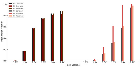
Figure 17.
Peak H2 and O2 molar fractions at various voltages for constant, stepwise, and reversed porosity profiles in the anode PTL.
4. Conclusions
This work presented a detailed analytical and numerical investigation of how porosity distribution strategies influence the performance of PEMWEs. Using a three-dimensional single-phase model, we examined the constant, linear, and stepwise porosity profiles applied to the anode and cathode porous layers. The simulations revealed that while porosity had minimal influence on performance at low voltages, its impact became more pronounced at higher voltages, particularly in the anode PTL, where oxygen build-up and transport resistance can significantly affect cell efficiency.
A key contribution of this study lies in the implementation of directional stepwise porosity profiles to mimic realistic manufacturing techniques such as dual-layer sintering or gradient compression. By modeling both standard (0.1 → 0.7) and reversed (0.7 → 0.1) stepwise gradients, we demonstrated that the position of the high-porosity zone plays a critical role in modulating gas transport behavior. The reversed configuration, with higher porosity near the membrane, led to reduced oxygen accumulation and slightly improved polarization performance compared to both the constant and standard stepwise profiles.
These findings underscore the significance of structured porosity design in optimizing PEMWE performance. Rather than relying solely on bulk material properties, this work emphasizes how localized porosity engineering can offer practical advantages in electrochemical systems. Although the present model is limited to single-phase simulations and does not account for gas saturation or species crossover, it provides a strong foundation for future multiphase analyses.
As PEMWEs move toward industrial-scale deployment, material reliability becomes increasingly critical. Recent insights by Leimbach et al. [41] and Kuhnert et al. [40] highlight how fatigue, corrosion, and mechanical degradation—particularly in bipolar plates—can influence system longevity and performance, urging closer integration between modeling and durability considerations.
In terms of application, the insights gained here extend beyond PEMWE to broader areas, such as fuel cell gas diffusion layers and porous electrodes in electrochemical reactors. The integration of mathematical modeling with microstructural design opens new possibilities for improving green hydrogen generation technologies through informed material engineering.
Future work will extend this approach to two-phase modeling, incorporating gas evolution, saturation, and dynamic operating conditions. Recent advances, such as those by Guan et al. [32], highlight the importance of incorporating multiphase transport effects to better capture performance limitations and water management challenges in PEMWEs. Furthermore, certain phenomena observed in this study—such as in-plane gas accumulation in Figure 9 and Figure 10—are artifacts of the single-phase framework and may deviate from realistic gas transport behavior. These will be addressed in future models that account for bubble dynamics and through-plane gas release mechanisms. In addition, future modeling efforts may benefit from incorporating dimensionless analysis—such as the Peclet, Damköhler, or Thiele modulus—to improve generalizability and deepen physical insight, especially in scaling studies. Future developments may also incorporate realistic porosity maps derived from advanced imaging techniques (e.g., X-ray tomography) to better capture local transport heterogeneities. Coupling the porosity distribution framework with optimization algorithms or data-driven tools may further accelerate the identification of high-performance electrode designs. Furthermore, the current model assumes isotropic transport in all porous layers and neglects the known anisotropy of fibrous PTLs, which can significantly affect through-plane and in-plane transport dynamics [20]. Additionally, the membrane is modeled as a fully dense ion-conducting region; future studies may explore how membrane porosity or nanoscale water channels could influence transport resistance and hydration dynamics.
Author Contributions
Conceptualization, A.B.; methodology, A.B.; software, A.B.; validation, A.B., S.C.S. and P.K.D.; formal analysis, A.B.; investigation, A.B.; resources, A.B.; data curation, A.B.; writing—original draft preparation, A.B.; writing—review and editing, S.C.S. and P.K.D.; visualization, A.B.; supervision, S.C.S. and P.K.D.; project administration, S.C.S.; funding acquisition, S.C.S. All authors have read and agreed to the published version of the manuscript.
Funding
This research received no external funding. The work was conducted as part of Ali Bayat’s PhD studies, supported by a doctoral scholarship from the University of Technology Sydney (UTS). The APC was funded by a fee waiver invitation extended to the corresponding author.
Data Availability Statement
The data supporting the findings of this study are available from the corresponding author upon reasonable request. No publicly archived datasets were used or generated during the current study.
Acknowledgments
The first author sincerely acknowledges the guidance and supervision of Suvash C. Saha and Prodip K. Das throughout the course of this research. Their technical insights and academic support were instrumental in shaping the direction and quality of this work. The author also appreciates the constructive feedback received during the internal review, which helped refine the manuscript prior to submission.
Conflicts of Interest
The authors declare no conflicts of interest. The funders had no role in the design of the study; in the collection, analysis, or interpretation of data; in the writing of the manuscript; or in the decision to publish the results.
Nomenclature
| List of symbols | |
| C | Kozeny–Carman Constant |
| Bulk Diffusivity | |
| Effective Diffusivity | |
| Pore Size | |
| Reversible Cell Potential | |
| Faraday Constant | |
| Volume Fractions of the CL | |
| Volume Fractions of the PTL | |
| CL thickness | |
| PTL Thickness | |
| Membrane Thickness | |
| Total Thickness of Layers | |
| Local Interfacial Current Density | |
| Exchange Current Density | |
| Pressure | |
| Universal Gas Constant | |
| . | Capillary Radius |
| S | Specific Surface Area |
| Local Gas Saturation | |
| Species Generation or Consumption Rate | |
| Momentum Source term | |
| Operating Temperature | |
| Velocity Field | |
| Pore Volume | |
| Total volume of the Porous Element | |
| z-Direction (Reference for Thickness) | |
| Transition Point | |
| Normalized Local Coordinate | |
| z-Position at Which Layer Begins | |
| Greek Symbols | |
| Anodic Transfer Coefficient | |
| Cathodic Transfer Coefficient | |
| Bruggeman Exponent | |
| Electrolyte Volume Fraction | |
| Porosity | |
| Overpotential | |
| Permeability | |
| Density | |
| Bulk Electrical Conductivity | |
| Effective Electrical Conductivity | |
| Effective Membrane Conductivity | |
| Effective Electrode Conductivity | |
| Viscosity | |
| Anode Electric Potential | |
| Cathode Electric Potential | |
| Electrode Potential | |
| Membrane Potential | |
Abbreviations
The following abbreviations are used in this manuscript:
| BP | Bipolar Plate |
| CFD | Computational Fluid Dynamics |
| CL | Catalyst Layer |
| PTL | Porous Transport Layer |
| GDL | Gas Diffusion Layer |
| H2 | Hydrogen |
| LBM | Lattice Boltzmann Method |
| Max | Maximum |
| Min | Minimum |
| MAE | Mean Absolute Error |
| MAPE | Mean Absolute Percentage Error |
| MEA | Membrane Electrode Assembly |
| O2 | Oxygen |
| PEM | Proton Exchange Membrane |
| PEMWE | Proton Exchange Membrane Water Electrolyzer |
| PTL | Porous Transport Layer |
| RMSE | Root Mean Square Error |
References
- Carmo, M.; Fritz, D.L.; Mergel, J.; Stolten, D. A comprehensive review on PEM water electrolysis. Int. J. Hydrogen Energy 2013, 38, 4901–4934. [Google Scholar] [CrossRef]
- Barbir, F. PEM electrolysis for production of hydrogen from renewable energy sources. Sol. Energy 2005, 78, 661–669. [Google Scholar] [CrossRef]
- Das, P.K.; Li, X.; Liu, Z.-S. Effective transport coefficients in PEM fuel cell catalyst and gas diffusion layers: Beyond Bruggeman approximation. Appl. Energy 2010, 87, 2785–2796. [Google Scholar] [CrossRef]
- Yuan, X.-Z.; Shaigan, N.; Song, C.; Aujla, M.; Neburchilov, V.; Kwan, J.T.H.; Wilkinson, D.P.; Bazylak, A.; Fatih, K. The porous transport layer in proton exchange membrane water electrolysis: Perspectives on a complex component. Sustain. Energy Fuels 2022, 6, 1824–1853. [Google Scholar] [CrossRef]
- Sohn, Y.-J.; Yim, S.-D.; Park, G.-G.; Kim, M.; Cha, S.-W.; Kim, K. PEMFC modeling based on characterization of effective diffusivity in simulated cathode catalyst layer. Int. J. Hydrogen Energy 2017, 42, 13226–13233. [Google Scholar] [CrossRef]
- Xu, Y.; Qiu, D.; Yi, P.; Lan, S.; Peng, L. An integrated model of the water transport in nonuniform compressed gas diffusion layers for PEMFC. Int. J. Hydrogen Energy 2019, 44, 13777–13785. [Google Scholar] [CrossRef]
- Shojaeefard, M.; Molaeimanesh, G.; Nazemian, M.; Moqaddari, M. A review on microstructure reconstruction of PEM fuel cells porous electrodes for pore scale simulation. Int. J. Hydrogen Energy 2016, 41, 20276–20293. [Google Scholar] [CrossRef]
- Benmehel, A.; Chabab, S.; Do Nascimento, A.; Chepy, M.; Kousksou, T. PEM Water Electrolyzer Modeling: Issues and Reflections. Energy Convers. Manag. X 2024, 21, 100738. [Google Scholar] [CrossRef]
- Bains, P.; Bennett, S.; Collina, L.; Connelly, E.; Delmastro, C.; Evangelopoulou, S.; Fajardy, M.; Gouy, A.; Kotani, M.; Le Marois, J. Global Hydrogen Review 2023; International Energy Agency: Paris, France, 2023. [Google Scholar]
- Das, P.K.; Jiao, K.; Wang, Y.; Barbir, F.; Li, X. Fuel Cells for Transportation: Fundamental Principles and Applications; Elsevier: Amsterdam, The Netherlands, 2023. [Google Scholar]
- Liu, R.-T.; Xu, Z.-L.; Li, F.-M.; Chen, F.-Y.; Yu, J.-Y.; Yan, Y.; Chen, Y.; Xia, B.Y. Recent advances in proton exchange membrane water electrolysis. Chem. Soc. Rev. 2023, 52, 5652–5683. [Google Scholar] [CrossRef]
- European Commission. REPowerEU Plan; European Commission: Brussels, Belgium, 2022. [Google Scholar]
- Stiber, S.; Sata, N.; Morawietz, T.; Ansar, S.; Jahnke, T.; Lee, J.K.; Bazylak, A.; Fallisch, A.; Gago, A.; Friedrich, K.A. A high-performance, durable and low-cost proton exchange membrane electrolyser with stainless steel components. Energy Environ. Sci. 2022, 15, 109–122. [Google Scholar] [CrossRef]
- Roshandel, R.; Farhanieh, B.; Saievar-Iranizad, E. The effects of porosity distribution variation on PEM fuel cell performance. Renew. Energy 2005, 30, 1557–1572. [Google Scholar] [CrossRef]
- Park, J.; Oh, H.; Lee, Y.I.; Min, K.; Lee, E.; Jyoung, J.-Y. Effect of the pore size variation in the substrate of the gas diffusion layer on water management and fuel cell performance. Appl. Energy 2016, 171, 200–212. [Google Scholar] [CrossRef]
- Zhang, Y.; Verma, A.; Pitchumani, R. Optimum design of polymer electrolyte membrane fuel cell with graded porosity gas diffusion layer. Int. J. Hydrogen Energy 2016, 41, 8412–8426. [Google Scholar] [CrossRef]
- Bruggeman, V.D. Berechnung verschiedener physikalischer Konstanten von heterogenen Substanzen. I. Dielektrizitätskonstanten und Leitfähigkeiten der Mischkörper aus isotropen Substanzen. Ann. Phys. 1935, 416, 636–664. [Google Scholar] [CrossRef]
- Jiang, Y.; Li, Y.; Ding, Y.; Hu, S.; Dang, J.; Yang, F.; Ouyang, M. Simulation and experiment study on two-phase flow characteristics of proton exchange membrane electrolysis cell. J. Power Sources 2023, 553, 232303. [Google Scholar] [CrossRef]
- Chen, L.; Wan, X.; Zhao, X.; Li, W.; Liu, X.; Zheng, L.; Liu, Q.; Yu, R.; Shui, J. Spatial porosity design of Fe–N–C catalysts for high power density PEM fuel cells and detection of water saturation of the catalyst layer by a microwave method. J. Mater. Chem. A 2022, 10, 7764–7772. [Google Scholar] [CrossRef]
- Gostick, J.T. Random Pore Network Modeling of Fibrous PEMFC Gas Diffusion Media Using Voronoi and Delaunay Tessellations. J. Electrochem. Soc. 2013, 160, F731–F743. [Google Scholar] [CrossRef]
- Chen, Z.; Yin, L.; Wang, Z.; Wang, K.; Ye, F.; Xu, C. Numerical simulation of parameter change in a proton exchange membrane electrolysis cell based on a dynamic model. Int. J. Energy Res. 2022, 46, 24074–24090. [Google Scholar] [CrossRef]
- Vu, H.T.; Tsotsas, E. A framework and numerical solution of the drying process in porous media by using a continuous model. Int. J. Chem. Eng. 2019, 2019, 9043670. [Google Scholar] [CrossRef]
- Rieder, D.R.; Peters, E.A.; Kuipers, J.A. Modeling the drying process of porous catalysts: Impact of the pore size distribution. Ind. Eng. Chem. Res. 2023, 62, 20006–20016. [Google Scholar] [CrossRef]
- Han, B.; Mo, J.; Kang, Z.; Zhang, F.-Y. Effects of membrane electrode assembly properties on two-phase transport and performance in proton exchange membrane electrolyzer cells. Electrochim. Acta 2016, 188, 317–326. [Google Scholar] [CrossRef]
- Salihi, H.; Ju, H. Two-Phase Modeling and Simulations of a Polymer Electrolyte Membrane Water Electrolyzer Considering Key Morphological and Geometrical Features in Porous Transport Layers. Energies 2023, 16, 766. [Google Scholar] [CrossRef]
- Østenstad, J. Multiphysical Modeling of a Next Generation PEM Electrolyser. Master’s Thesis, NTNU, Trondheim, Norway, 2023. [Google Scholar]
- Wang, Y.; Diaz, D.F.R.; Chen, K.S.; Wang, Z.; Adroher, X.C. Materials, technological status, and fundamentals of PEM fuel cells–a review. Mater. Today 2020, 32, 178–203. [Google Scholar] [CrossRef]
- Ruiz, D.D.H.; Sasmito, A.P.; Shamim, T. Numerical investigation of the high temperature PEM electrolyzer: Effect of flow channel configurations. ECS Trans. 2013, 58, 99. [Google Scholar] [CrossRef]
- Toghyani, S.; Afshari, E.; Baniasadi, E. Three-dimensional computational fluid dynamics modeling of proton exchange membrane electrolyzer with new flow field pattern. J. Therm. Anal. Calorim. 2019, 135, 1911–1919. [Google Scholar] [CrossRef]
- Bayat, A.; Das, P.K.; Saha, G.; Saha, S.C. Optimizing Proton Exchange Membrane Electrolyzer Cells: A Comprehensive Parametric Analysis of Flow, Electrochemical, and Geometrical Factors. Int. J. Thermofluids 2025, 27, 101177. [Google Scholar] [CrossRef]
- Ubong, E.; Shi, Z.; Wang, X. Three-dimensional modeling and experimental study of a high temperature PBI-based PEM fuel cell. J. Electrochem. Soc. 2009, 156, B1276. [Google Scholar] [CrossRef]
- Guan, X.; Bai, J.; Zhang, J.; Yang, N. Multiphase flow in PEM water electrolyzers: A mini-review. Curr. Opin. Chem. Eng. 2024, 43, 100988. [Google Scholar] [CrossRef]
- Corda, G.; Cucurachi, A.; Fontanesi, S.; d’Adamo, A. Three-Dimensional CFD Simulation of a Proton Exchange Membrane Electrolysis Cell. Energies 2023, 16, 5968. [Google Scholar] [CrossRef]
- Bayat, A.; Das, P.K.; Saha, G.; Saha, S.C. Proton Exchange Membrane Electrolysis Revisited: Advancements, Challenges, and Two-Phase Transport Insights in Materials and Modelling. Eng 2025, 6, 72. [Google Scholar] [CrossRef]
- Ma, Z.; Witteman, L.; Wrubel, J.A.; Bender, G. A comprehensive modeling method for proton exchange membrane electrolyzer development. Int. J. Hydrogen Energy 2021, 46, 17627–17643. [Google Scholar] [CrossRef]
- Nie, J.; Chen, Y.; Cohen, S.; Carter, B.D.; Boehm, R.F. Numerical and experimental study of three-dimensional fluid flow in the bipolar plate of a PEM electrolysis cell. Int. J. Therm. Sci. 2009, 48, 1914–1922. [Google Scholar] [CrossRef]
- Lee, J.K.; Lau, G.Y.; Sabharwal, M.; Weber, A.Z.; Peng, X.; Tucker, M.C. Titanium porous-transport layers for PEM water electrolysis prepared by tape casting. J. Power Sources 2023, 559, 232606. [Google Scholar] [CrossRef]
- Altus, S.J.; Inkson, B.J.; Hack, J. Complementary X-ray and neutron imaging of water electrolysers for green hydrogen production. J. Mater. Chem. A 2024, 12, 23364–23391. [Google Scholar] [CrossRef]
- Huang, Y.-X.; Cheng, C.-H.; Wang, X.-D.; Jang, J.-Y. Effects of porosity gradient in gas diffusion layers on performance of proton exchange membrane fuel cells. Energy 2010, 35, 4786–4794. [Google Scholar] [CrossRef]
- Kuhnert, E.; Heidinger, M.; Sandu, D.; Hacker, V.; Bodner, M. Analysis of PEM Water Electrolyzer Failure Due to Induced Hydrogen Crossover in Catalyst-Coated PFSA Membranes. Membranes 2023, 13, 348. [Google Scholar] [CrossRef]
- Leimbach, M.; Kurniawan, M.; Fritz, M.; Bund, A. Electrodeposition and Characterization of Platinum Coatings on Titanium Porous Transport Layers for PEM Electrolyzers. Meet. Abstr. Electrochem. Soc. 2024, MA2024-02, 1901. [Google Scholar] [CrossRef]
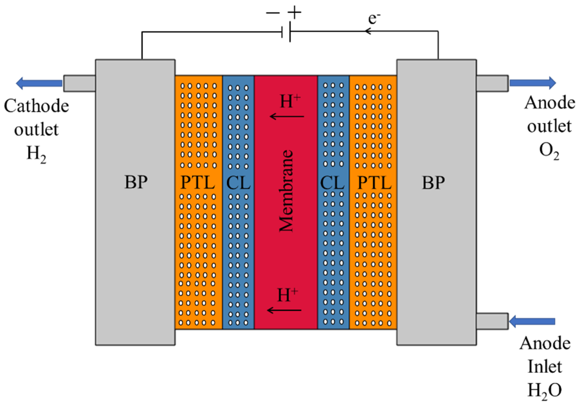
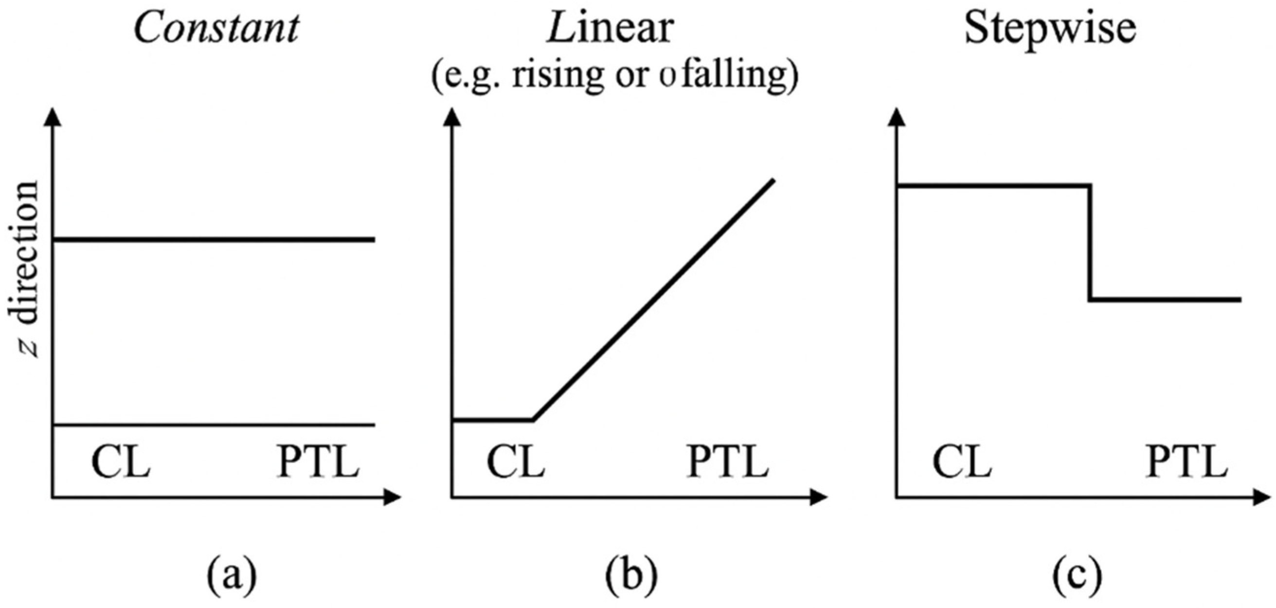

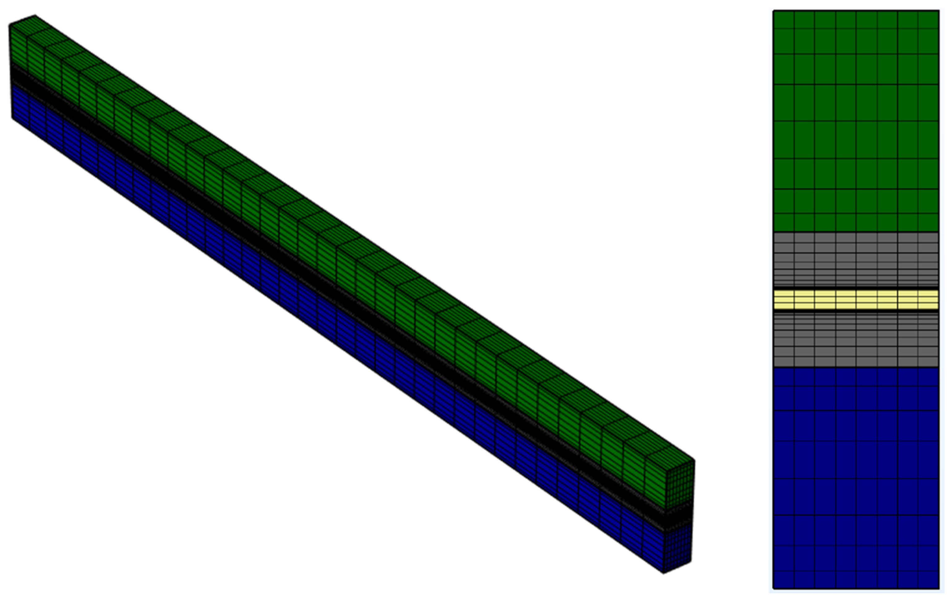
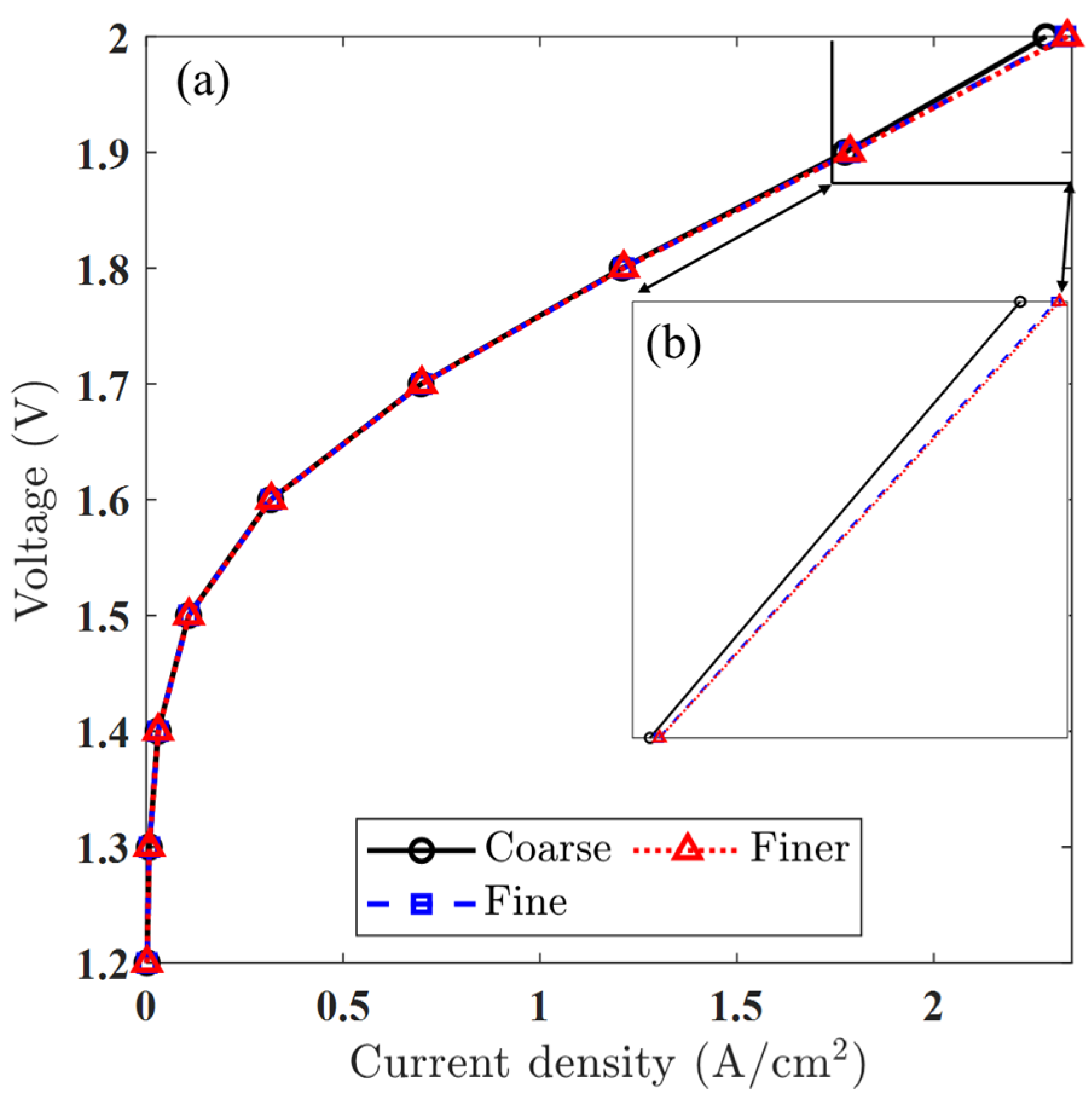
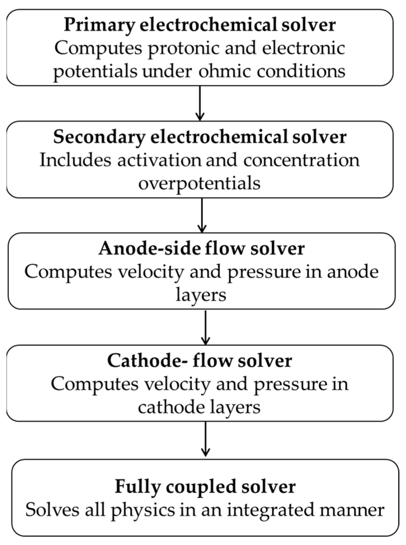
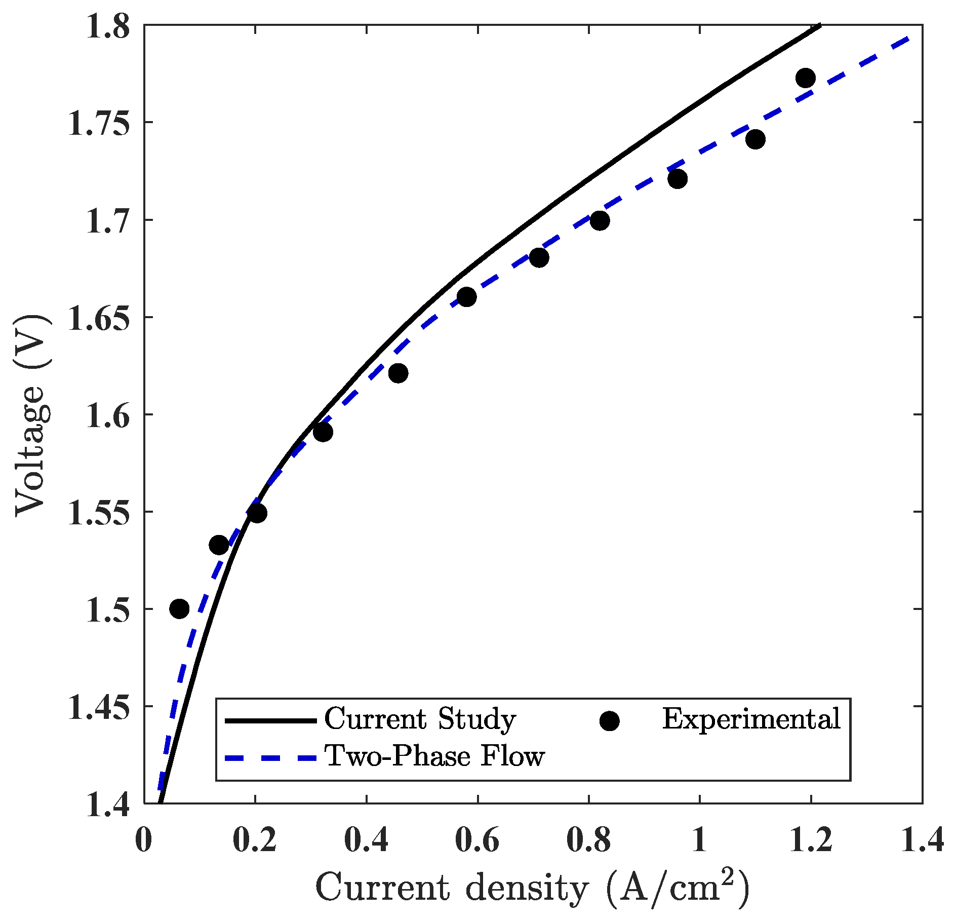
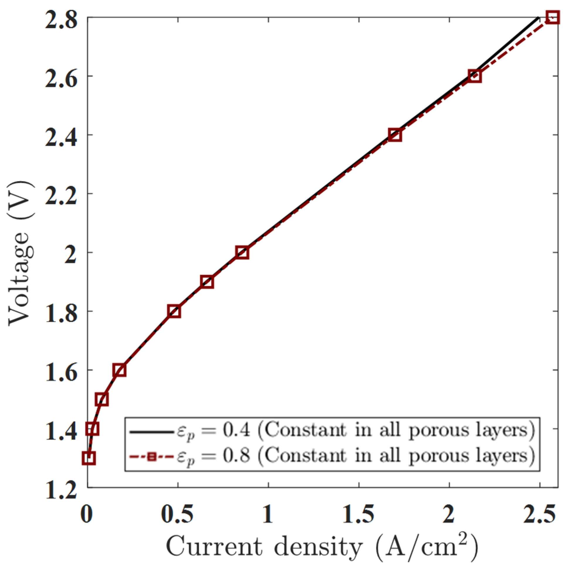
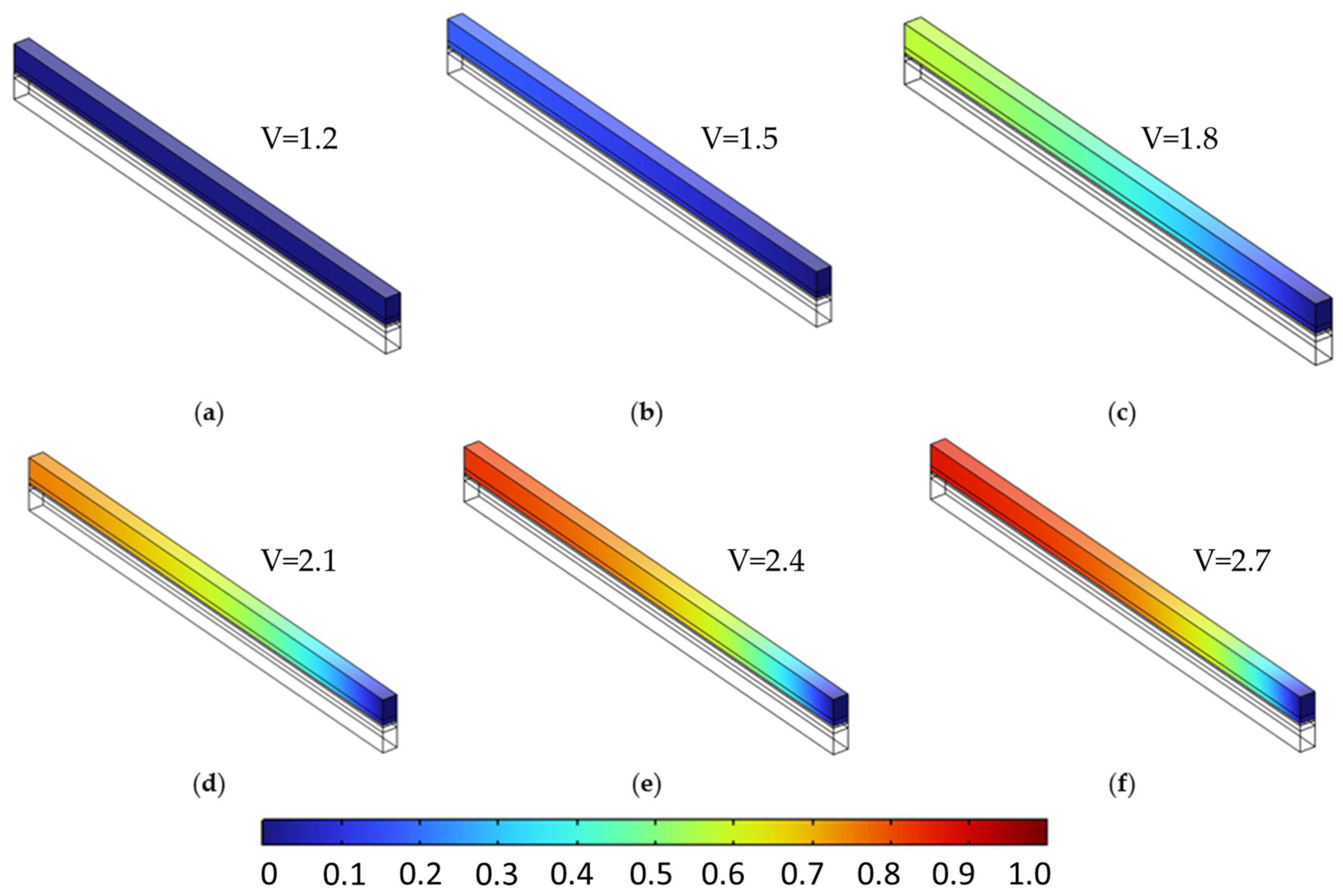

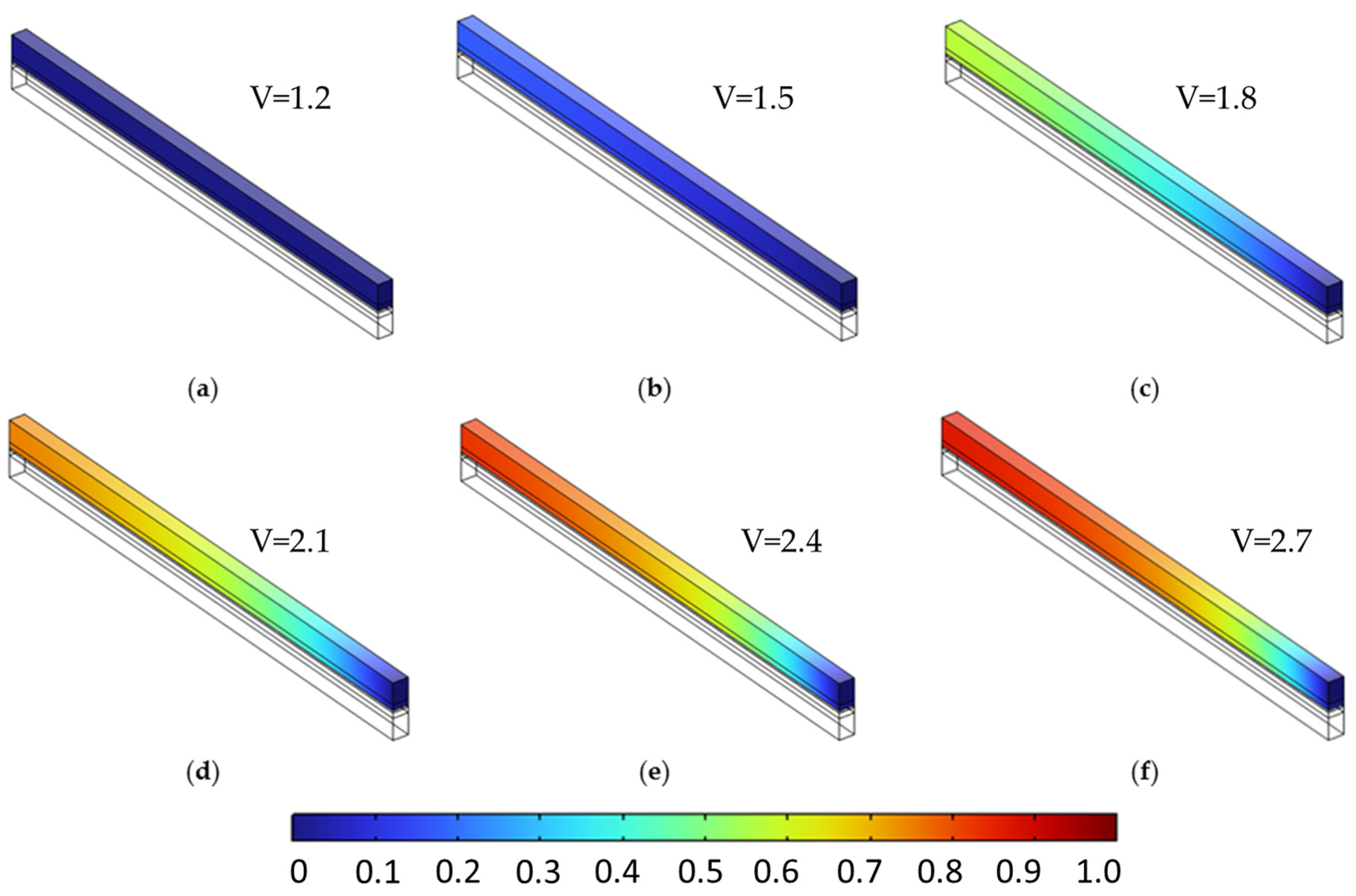

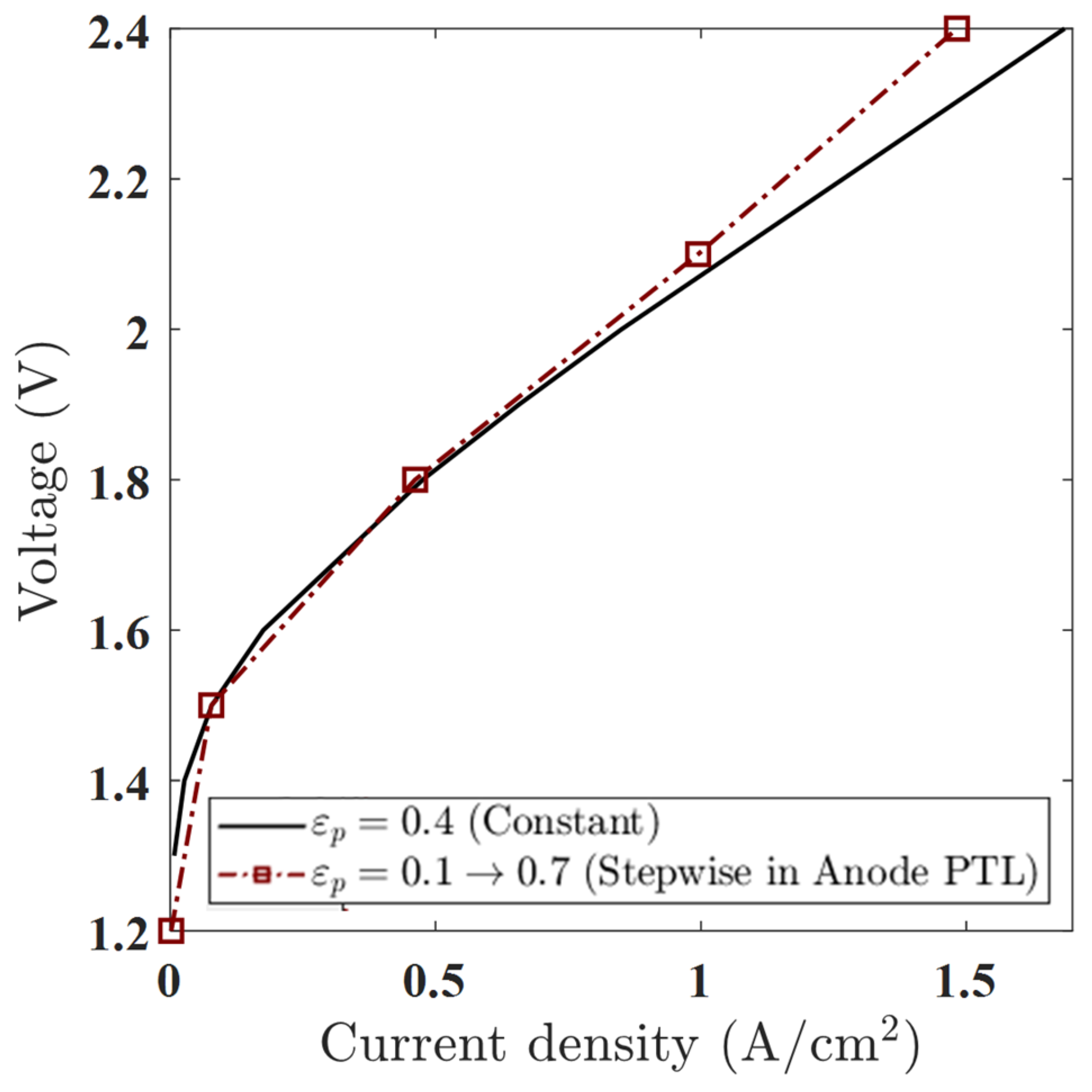
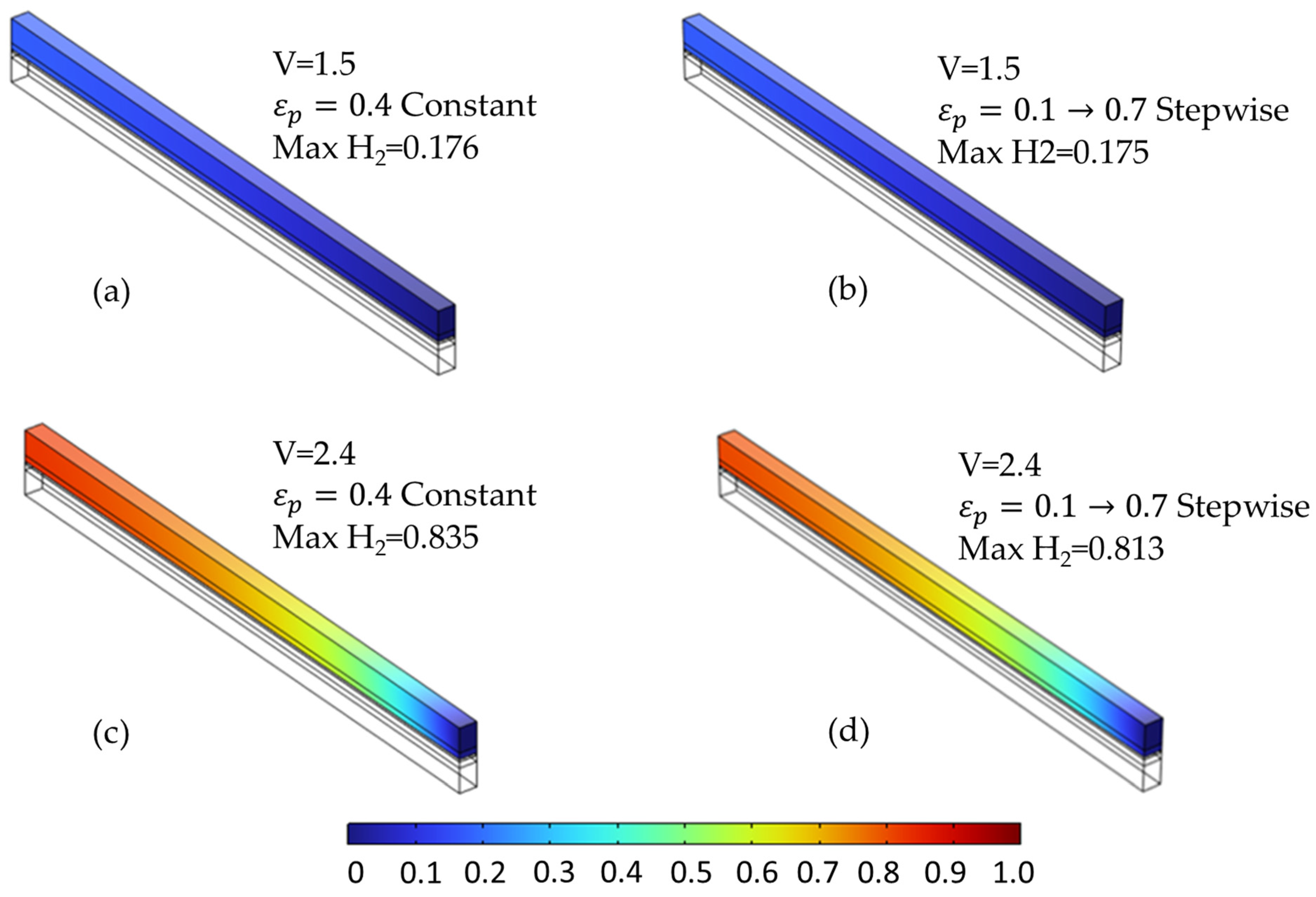
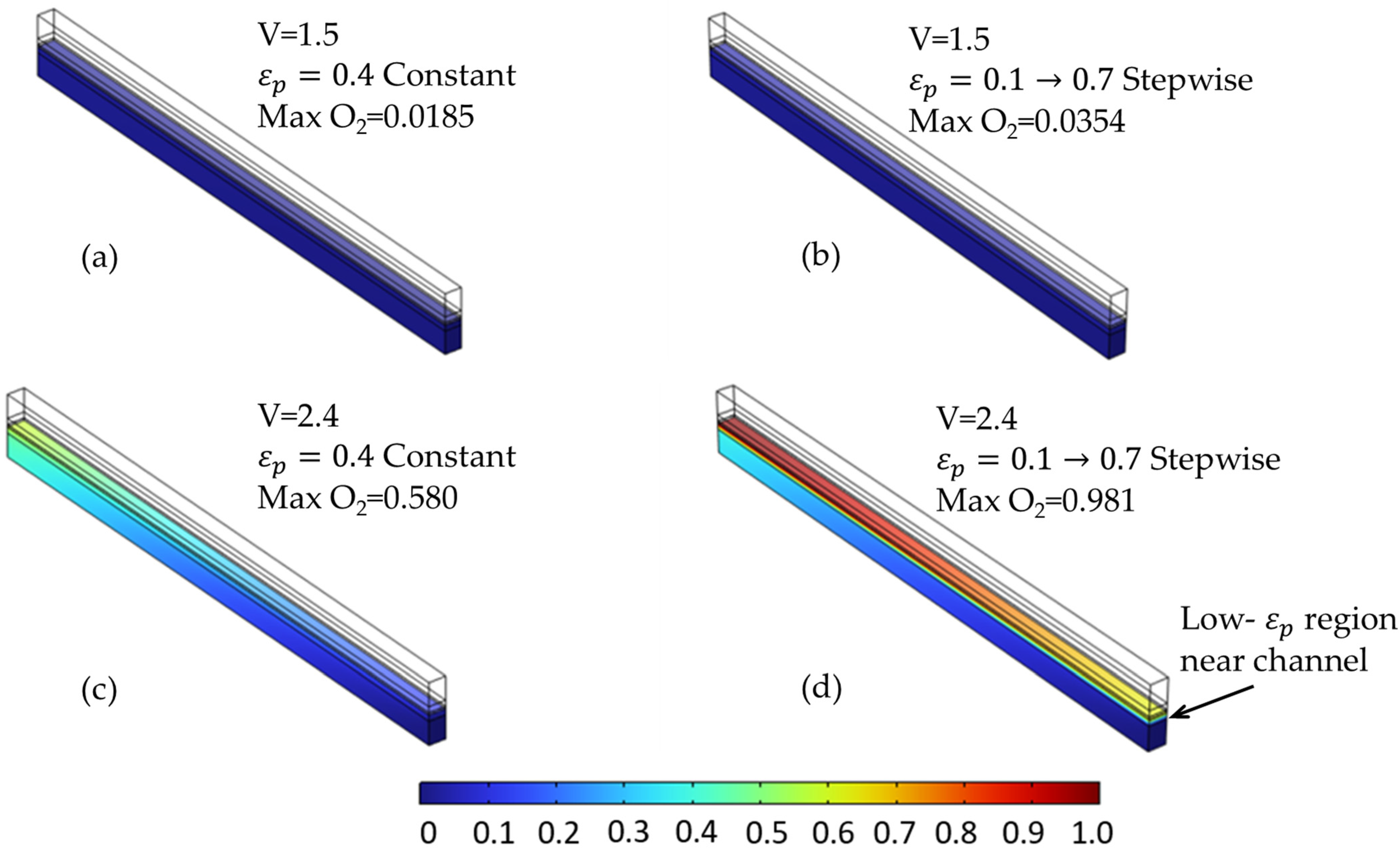
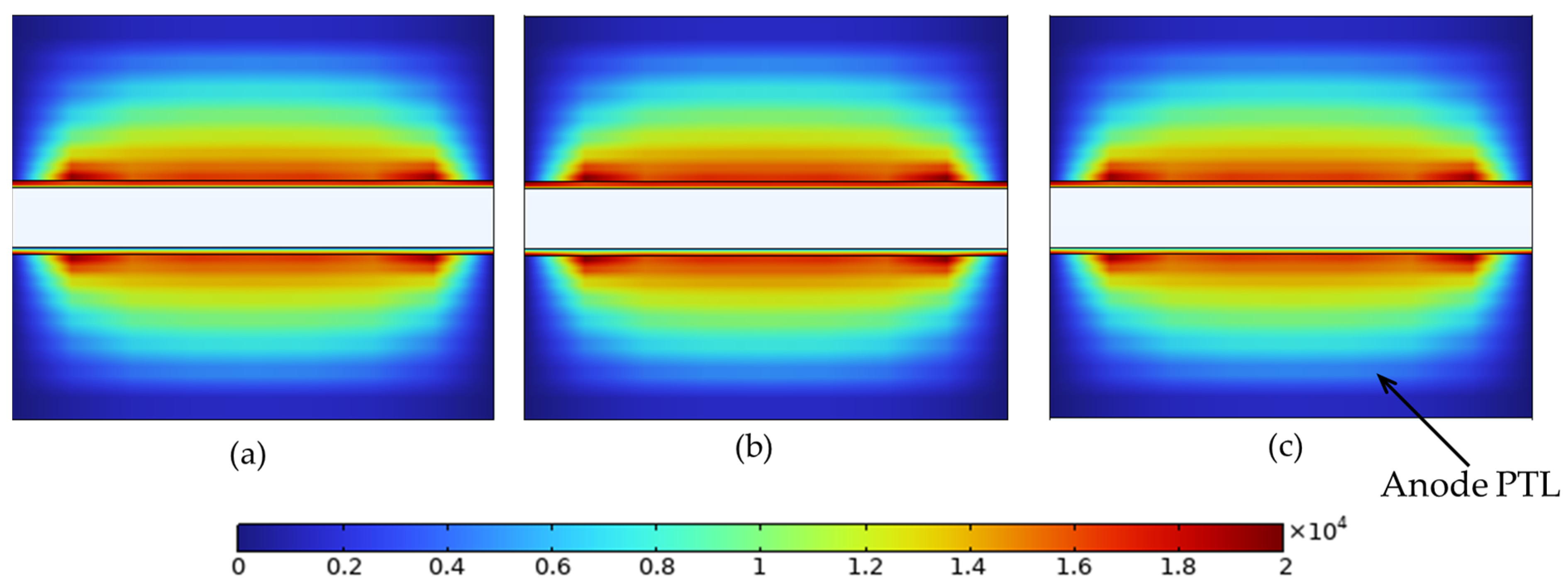


Disclaimer/Publisher’s Note: The statements, opinions and data contained in all publications are solely those of the individual author(s) and contributor(s) and not of MDPI and/or the editor(s). MDPI and/or the editor(s) disclaim responsibility for any injury to people or property resulting from any ideas, methods, instructions or products referred to in the content. |
© 2025 by the authors. Licensee MDPI, Basel, Switzerland. This article is an open access article distributed under the terms and conditions of the Creative Commons Attribution (CC BY) license (https://creativecommons.org/licenses/by/4.0/).