From Inequality to Extremes and Back: A Lorenz Representation of the Pickands Dependence Function

Abstract

We establish a correspondence between Lorenz curves and Pickands dependence functions, thereby reframing the construction of any bivariate extreme-value copula as an inequality problem. We discuss the conditions under which a Lorenz curve generates a closed-form Pickands model, considerably expanding the small set of tractable parametrizations currently available. Furthermore, the Pickands measure-generating function M can be written explicitly in terms of the quantile function underlying the Lorenz curve, providing a constructive route to model specification. Finally, classical inequality indices like the Gini coincide with scale-free, rotation-invariant indices of global upper-tail dependence, thereby complementing local coefficients such as the upper tail dependence index ${\lambda }_U$.

1. Introduction

Quantifying how often and how severely extreme events strike together is a central task in financial risk management and insurance but also in the natural sciences [1,2].

For the bivariate case, extreme-value copulas provide the canonical modeling framework [3,4]. Interestingly, their dependence structure is fully characterized by a single convex curve inside the unit square, the Pickands dependence function P(u) [4,5,6]. Yet the practical application of extreme-value copulas has long been constrained by a significant bottleneck. Despite its theoretical elegance, the universe of known parametric families for P(u) remains remarkably small. This scarcity limits practical use whenever the amount and quality of data do not support fully nonparametric estimators [7,8,9], creating a difficult trade-off between overly simplistic models and data-intensive nonparametric methods, a challenge that is particularly acute in fields like climate-related financial risks [10].

A parallel literature on economic inequality studies the Lorenz curve, another convex curve in the unit square, for which decades of work have produced many tractable parametrizations and ready-made indices [11,12,13]. This rich, well-established mathematical toolkit, we argue, holds the key to overcoming the aforementioned limitations in the parametric modeling of the Pickands dependence function.

The primary objective of this paper is to bridge the gap between inequality measurement and extreme-value theory, thereby providing a new, systematic engine for generating dependence models. We show that rotating the “Pickands triangle” by 45° and rescaling establishes a bijective map between Pickands and Lorenz curves. When some conditions are met, the map turns a Lorenz family into a closed-form Pickands model, and vice versa, thus systematically enlarging the catalog of tractable extreme-value copulas. Our work yields three further key innovations. First, the measure-generating function M of Pickands [6] can be written explicitly in terms of the quantile function underlying the Lorenz curve, providing a constructive route to model specification irrespective of the inversion method. Second, classical inequality distances (e.g., the Gini and Pietra indices [14]) translate into scale-free, rotation-invariant indices of global upper-tail dependence that complement local coefficients such as the index of upper-tail dependence ${\lambda }_U$ [4]. Finally, our framework provides a clear economic interpretation for tail dependence, linking it directly to the concentration of risk. The use of Lorenz curves in dealing with copulas is not new [15], but—to the best of our knowledge—this is the first attempt to use them in the realm of extreme-value copulas.

The usefulness of the Lorenz–Pickands link in financial risk management is supported by a growing body of empirical evidence on joint extremes. A seminal study [16] showed how upper-tail dependence between major equity markets surges during crashes, challenging the efficacy of geographical diversification, and suggesting the use of extreme-value copulas. In [17], the authors introduced diagnostics that compare fitted extreme-value surfaces with alternative copulas and documented that episodes of heightened tail co-movement coincide with higher risk premia and diminished hedging power. Subsequent work by [18] quantified the economic stakes: switching from an elliptical to an extreme-value copula can raise the 99% Value-at-Risk of a diversified equity–bond portfolio by up to 30%, materially affecting capital requirements. Dynamic specifications that marry GARCH margins with conditional extreme-value copulas further improve forecasts of joint exceedances and back-testing performance [19,20]. In derivative pricing, basket and spread options valued under an extreme-value dependence structure reproduce observed tail-wing premiums better than Gaussian benchmarks [21], reducing bid–ask disparities in energy and FX markets. Beyond market risk, [22] applied covariate-dependent extreme-value copulas to operational losses, producing coherent business-line capital figures under the Basel framework. Empirical evidence also reveals that equity returns and implied volatility share common jumps [23], commodity-linked credit exposures exhibit “wrong-way” behavior [24], and regional catastrophe losses display marked spatial concentration [25].

Together all these studies underscore that whenever simultaneous extremes matter for value—be it market, credit, or operational—extreme-value copulas capture the economics of contagion more faithfully than competing dependence models, and thus the study of the Pickands function becomes particularly relevant. Within our framework, any extreme-value copula becomes a problem we can tackle in the inequality space, providing additional tools for the analysis of the Pickands function, tail dependence, stress-testing, and decision making. Our work aims to provide the explicit mathematical machinery to make this connection rigorous and readily applicable, open the path—we hope—for further research.

This paper is organized as follows. Section 2 revisits Pickands and Lorenz curves under a unified geometric lens. Section 3 introduces the Lorenz–Pickands equivalence geometrically and via the so-called Gini coordinate system. Section 4 covers examples of existing and new parametric families of Pickands functions via the Lorenz representation. Section 5 deals with those situations in which either the Pickands or the Lorenz cannot be obtained in closed form. Section 6 discusses the use of inequality indices in the context of tail dependence. Section 7 is devoted to a measure-theoretic and constructive representation of the Pickands function via Lorenz curves. Section 8 provides a novel representation of extreme-value copulas using the Lorenz–Pickands relation. Section 9 provides an example of the use of the Pickands-Lorenz connection on actual financial data. Section 10 concludes and opens paths for further research.

2. Preliminaries

In this section we recall the basics about the two curves we build our contribution upon: the Pickands dependence function [5,26] and the Lorenz curve [11].

2.1. Extreme-Value Copulas and the Pickands Dependence Function

Copulas are an elegant way of representing multivariate distributions, by focusing attention on the embedded dependence structure. Thanks to Sklar’s theorem [27], the joint distribution J of a bivariate random vector $(Y,Z)$ can be given as the combination of the marginal distributions $F\left(y\right)$ and $G\left(z\right)$ of Y and Z, and of a function C called copula, such that

$$J(y,z)=C\left(F\right(y),G(z\left)\right).$$

The function C essentially accounts for the dependence between Y and Z, separating the joint behavior from the margins, and we refer to [3] for a nice introduction. However, it is worth noticing that some scholars argue that the very act of separating the marginal distributions from the dependence structure using a copula can lead to an oversimplified and potentially misleading understanding of how variables truly interact, especially in a dynamic framework [28].

Extreme-value copulas arise as the possible limit of copulas of component-wise maxima of i.i.d. (or strongly mixing stationary [29]) random sequences [4,8]. These copulas prove to be extremely useful in risk management, to model joint extremes, or when dealing with data characterized by positive and possibly asymmetric dependence [1,2,16].

In the bivariate case, a copula C is an extreme-value copula if and only if it can be represented as

$$C\left(y^{1-u},y^u\right)=y^{P\left(u\right)},y,u\in [0,1],$$

(1)

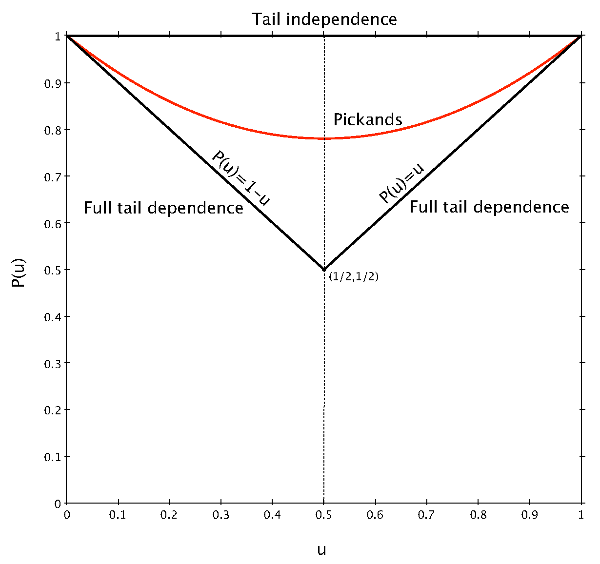
where $P:[0,1]\to [1/2,1]$ is a convex function, called Pickands dependence function [5], satisfying

$$max(u,1-u)\le P\left(u\right)\le 1.$$

when $P\left(u\right)=1$ for every $u\in [0,1]$, the random variables Y and Z are completely tail independent. Conversely, when $P\left(u\right)=u$ or $P\left(u\right)=1-u$, we are in the case of perfect tail dependence. For all values of $P\left(u\right)$ in between, different degrees of tail dependence are reached [6,8]. In Figure 1 a graphical representation of $P\left(u\right)$ is given, where we see that the Pickands dependence function lives in the so-called Pickands triangle of vertices $(0,1)$, $(1/2,1/2)$, and $(1,1)$.

Knowing the Pickands dependence function $P\left(u\right)$ is particularly useful when dealing with bivariate extreme-value copulas. In fact, as is clear from Equation (1), all the statistical inference on the copula C and its dependence structure can be reduced to the inference on its Pickands function [4].

2.2. The Lorenz Curve

Introduced by Max Lorenz in 1905 [11], the Lorenz curve is a fundamental tool in the study of economic inequality and the distribution of wealth in the society [30,31].

Consider a positive random variable X with continuous distribution function $F\left(x\right)$, quantile function $Q\left(\alpha \right)$ and mean ${\mu }_X=\mathbb{E}\left(X\right)<\infty$. The Lorenz curve $L\left(p\right)\in [0,1]$ is commonly defined as

$$L\left(p\right)={\displaystyle \frac{{\int }_0^{p}Q\left(\alpha \right)d\alpha }{{\mu }_X}},p\in [0,1].$$

(2)

By construction the Lorenz curve is a convex increasing function that lies in the unit square, with $L\left(0\right)=0$ and $L\left(1\right)=1$ such that $p\ge L\left(p\right)$. In terms of wealth distribution, the Lorenz curve tells us that $p\%$ of the population owns $L\left(p\right)\%$ of the total wealth in the economy [30], when wealth is distributed according to $F\left(x\right)$.

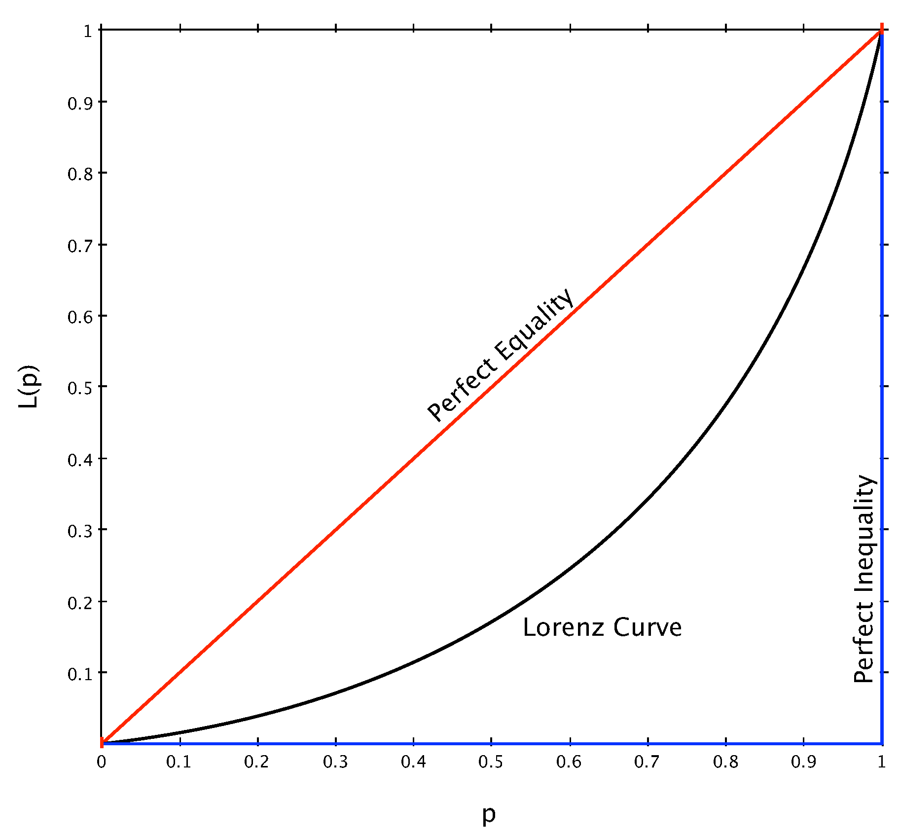
The curve $L\left(p\right)$ is bounded from above by the so-called perfect equality line, i.e., the anti-diagonal of the unit square defined as $L_{PE}\left(p\right)=p$, and from below by the perfect inequality line, defined as $L_{PI}\left(p\right)=0$ for $0\le p<1$ and $L_{PI}\left(p\right)=1$ for $p=1$. The curve $L_{PE}$ represents the ideal situation in which every single individual in the economy possesses the exact same amount of wealth (i.e., there is no variability), while $L_{PI}$ indicates that one individual owns everything and all the others nothing (maximum variability). The Lorenz curve and its bounds are given in Figure 2.

It is worth noticing that any convex increasing function defined within the triangle of vertices $(0,0),(1,1),(0,1)$, and such that $L\left(0\right)=0$ and $L\left(1\right)=1$, is actually a Lorenz curve [32], and given Equation (2) it thus characterizes a given distribution function up to its mean.

Over the years, a huge variety of summary statistics have been developed to express specific features of the Lorenz curve. One of the most important examples is the family of concentration indices [13], measuring the distance between the Lorenz curve and the perfect equality line. In more formal terms, a concentration (or distance or inequality) index is defined as

$$I_d={\displaystyle \frac{{∥L\left(p\right)-L_{PE}\left(p\right)∥}_d}{{∥L_{PI}\left(p\right)-L_{PE}\left(p\right)∥}_d}},$$

(3)

where the denominator is for normalization, so that $0\le I_d\le 1$ for all $d\in [1,\infty ]$.

High values of $I_d$ signal high variability in the data, leading to a high concentration of the wealth induced by the distribution $F\left(x\right)$. Therefore, when $I_d=1$ the random variable X reaches its maximum variability. Conversely, low values of $I_d$ signal low variability in the data, leading to a low concentration of wealth. When $I_d=0$, X is nothing but a constant.

From Equation (3) it is clear that, by varying the type of distance ${∥·∥}_d$, we can define different indices: the famous Gini index [33,34] is obtained by fixing $d=1$, while the Pietra index is obtained when $d=\infty$ [35].

Additional measures one can derive from $L\left(p\right)$ are related to its curvature and to its length and other geometric properties of the curve. We suggest [13,30] for more details.

3. From Pickands to Lorenz and Back

In Figure 1 the Pickands dependence function appears as a convex function embedded in the right triangle with vertices $(0,1)$, $(1/2,1/2)$, and $(1,1)$.

Now, imagine first rotating this triangle counterclockwise by pivoting on the (1,1) vertex, until the segment $\overline{(0,1)(1,1)}$ lies on the diagonal $\overline{(0,0)(1,1)}$. This corresponds to a 45-degree rotation. Then inflate all the edges of the triangle by a factor of $1/\sqrt{2}$, to make them unit length, thus also stretching the Pickands function within. The new triangle now coincides with the triangle of vertices (0,0), (1,0), and (1,1), and the convex, stretched, and now non-decreasing Pickands function can itself be seen as a Lorenz curve.

An immediate consequence of this geometrical transformation is that every Pickands function defines a unique Lorenz curve, but also that every Lorenz curve corresponds to a given Pickands function (the correspondence is one-to-one, as we shall see). This simple observation gives us the possibility of studying tail dependence using several tools from inequality studies, and to easily generate parametric families of Pickands functions by using the many Lorenz curves available in the literature.

The rotation and inflation procedure we have just described is useful to have an immediate understanding of the link between the Pickands dependence function and the Lorenz curve. However, it is not difficult to see that this rotation will generally give an implicit representation of one curve in terms of the other. This is due to the fact that the axes are not preserved. The u-axis of the Pickands function in Figure 1 does not correspond to the $p$-axis of the Lorenz curve in Figure 2. In fact, after rotation, the u-axis is parallel to the perfect equality line. For this reason, an alternative transformation of the Lorenz curve will prove more useful.

3.1. Remapping the Lorenz Curve

Let us consider an alternative representation of the Lorenz curve, in terms of the orthogonal distance of every point of $L\left(p\right)$ from the perfect equality line $L_{PE}=p$. This perspective on the Lorenz curve connects to the Gini coordinate system, a framework originally introduced by Corrado Gini [36] that remains underutilized and relatively obscure in the modern economic inequality literature, largely because his foundational work was primarily published in Italian during the first decades of the 20th century.

As we show in Section 7, a very interesting feature of this alternative representation is that it naturally embeds a way of characterizing the measure generating function M of the Pickands function [6], in terms of the quantile function of any positive valued random variable with a finite mean.

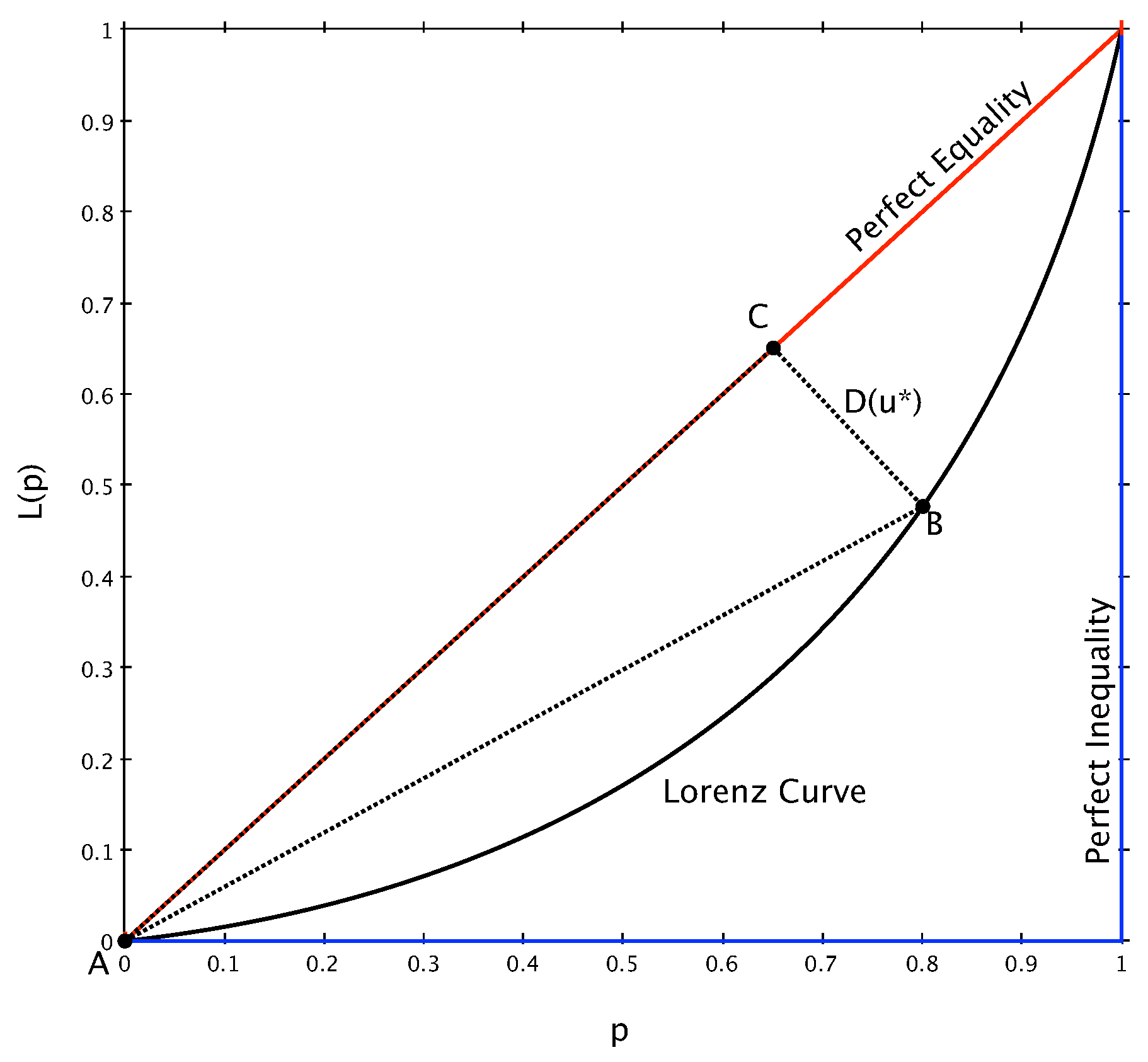
In Figure 3 imagine we are interested in computing the length of the segment $\overline{CB}$, corresponding to the orthogonal distance of point B on $L\left(p\right)$ from the perfect equality line. By first computing segments $\overline{AB}$ and $\overline{AC}$, we can easily apply the Pythagorean theorem to obtain $\overline{CB}$.

Let us consider a family of lines that are orthogonal to the perfect equality line, and that we can define $y=-p+2u$, with $u\in [0,1]$. In Figure 3, we can imagine that one of these lines, for $u=u^{*}$, passes through points B and C.

To find the length of $\overline{AC}$ we first solve the system

$$\left\{\begin{array}{c}y=-p+2u^{*}\hfill \\ y=p\hfill \end{array}\right.,$$

to obtain point C, and from this we get $\overline{AC}=u\sqrt{2}$. Similarly, we can find the length of $\overline{AB}$ starting from

$$\left\{\begin{array}{c}y=-p+2u^{*}\hfill \\ y=L\left(p\right)\hfill \end{array}\right..$$

To solve this system it is convenient to introduce the quantity

$$K\left(p\right):={\displaystyle \frac{1}{2}}\left(L\left(p\right)+p\right),$$

(4)

so that we have

$$\left\{\begin{array}{c}K\left(p\right)=u^{*}\hfill \\ y=-p+2u^{*}\hfill \end{array}\right..$$

(5)

The quantity $K\left(p\right)$ of Equation (4) is nothing but the simple arithmetic mean of two Lorenz curves, $L\left(p\right)$ and $L_{PE}\left(p\right)=p$.

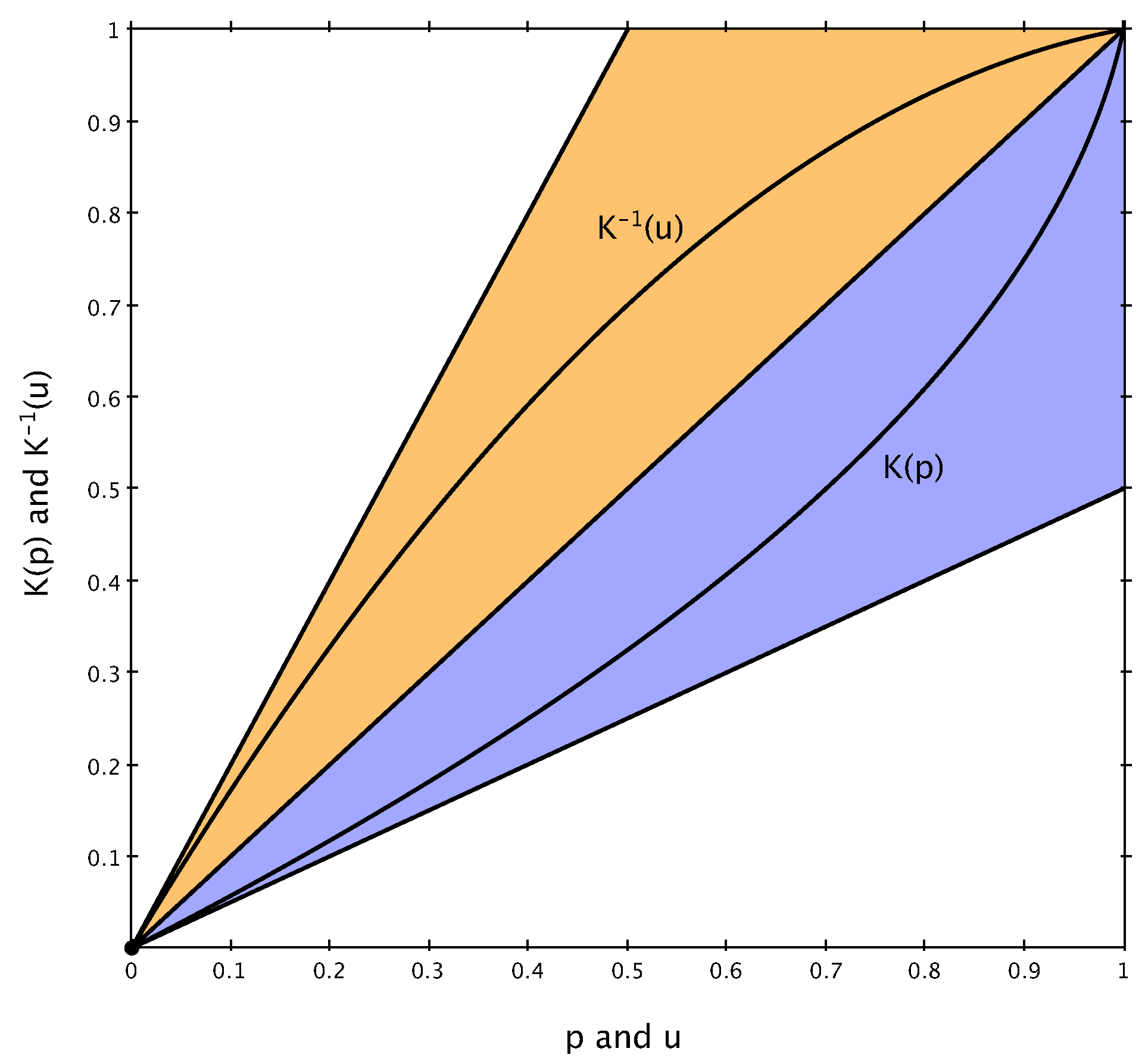
Proposition 1 clarifies some interesting properties of both $K\left(p\right)$ and its inverse $K^{-1}\left(u\right)$, and Figure 4 shows their behavior in the unit square.

Proposition 1. 

Let $L\left(p\right)$, $p\in [0,1]$, be a Lorenz curve and set $K\left(p\right)={\displaystyle \frac{1}{2}}\left(L\left(p\right)+p\right)$. Then:

1 

K is a Lorenz curve satisfying $p/2\le K\left(p\right)\le p$ for all $p\in [0,1]$;

2 

K is strictly increasing and convex on $[0,1]$, and its inverse $K^{-1}\left(u\right)$ exists, is unique, and concave;

3 

For all $u\in [0,1]$, it holds that $u\le K^{-1}\left(u\right)\le 2u$.

Proof. 

By definition, $K\left(p\right)$ is the average of $L\left(p\right)$ and p. Since L is a Lorenz curve, we have $0\le L\left(p\right)\le p$ for all $p\in [0,1]$, and $L\left(0\right)=0$, $L\left(1\right)=1$. Thus, for all $p\in [0,1]$,

$${\displaystyle \frac{p}{2}}={\displaystyle \frac{0+p}{2}}\le K\left(p\right)={\displaystyle \frac{L\left(p\right)+p}{2}}\le {\displaystyle \frac{p+p}{2}}=p.$$

Moreover, $K\left(0\right)={\displaystyle \frac{L\left(0\right)+0}{2}}=0$ and $K\left(1\right)={\displaystyle \frac{L\left(1\right)+1}{2}}=1$, so K shares the same endpoints as a Lorenz curve. Convex combinations of Lorenz curves are again Lorenz curves (see [37]), and since K is a convex combination of L and the identity $p\mapsto p$, it follows that K is itself a Lorenz curve.

Because L is continuous, convex, and increasing, the sum $L\left(p\right)+p$ is strictly increasing, and so is $K\left(p\right)$. Since the identity $p\to p$ is linear, K inherits convexity from L. As K is strictly increasing and continuous on $[0,1]$, it is invertible on its image $[0,1]$, and the inverse $K^{-1}$ is also continuous and increasing. The concavity of $K^{-1}$ follows from the general result that the inverse of a convex, strictly increasing function is concave.

Since $p\mapsto K\left(p\right)$ satisfies $p/2\le K\left(p\right)\le p$ for all $p\in [0,1]$, we can write the following: $K\left(p\right)\ge {\displaystyle \frac{p}{2}}$ and $K\left(p\right)\le p$. Let $u=K\left(p\right)$. Rewriting the inequalities in terms of p gives the following:

$$K\left(p\right)\ge {\displaystyle \frac{p}{2}}\Rightarrow p\le 2u,K\left(p\right)\le p\Rightarrow u\le p.$$

Therefore, for $p=K^{-1}\left(u\right)$, we get the following:

$$u\le K^{-1}\left(u\right)\le 2u.$$

   □

Now, coming back to Equation (5), we find a solution for $p=K^{-1}\left(u^{*}\right)$ and $y=-K^{-1}\left(u^{*}\right)+2u^{*}$, and

$$\overline{AB}=\sqrt{2K^{-1}\left(u^{*}\right)+{\left(2u^{*}\right)}^2-4K^{-1}\left(u^{*}\right)u^{*}}.$$

A simple application of the Pythagorean theorem then tells that

$$\overline{CB}=D\left(u^{*}\right)=\sqrt{2}|K^{-1}\left(u^{*}\right)-u^{*}|.$$

(6)

For different points B and C in Figure 3, one will find different values of u defining the orthogonal distance $D\left(u\right)$. In general, for $u\in [0,1]$, it is easy to verify that $D\left(u\right)\in \left[0,{\displaystyle \frac{\sqrt{2}}{2}}\right]$.

Removing the factor $\sqrt{2}$ from $D\left(u\right)$, let us define

$$\overline{D}\left(u\right)=|K^{-1}\left(u\right)-u|=K^{-1}\left(u\right)-u,$$

(7)

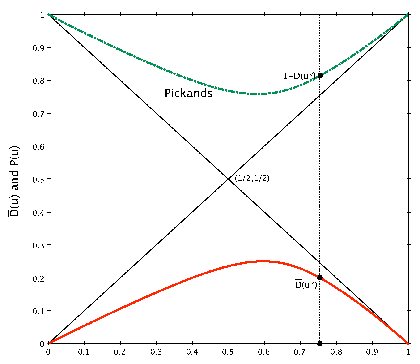
where the possibility of removing the absolute value comes from the fact that $K^{-1}\left(u\right)\ge u$. Therefore, $\overline{D}\left(u\right)$ is a concave function like the one in Figure 5, lying in the triangle of vertices (0,0), (1/2,1/2), and (1,0), with $\overline{D}\left(0\right)=0$ and $\overline{D}\left(1\right)=0$. It represents a remapping of a Lorenz curve in the Gini coordinate system [36].

3.2. A New Representation of the Pickands Dependence Function

By mirroring the function $\overline{D}\left(u\right)$ in the triangle of vertices (1,0), (1/2,1/2), and (1,1), we easily find a new convenient way of defining Pickands dependence functions. In fact

$$P\left(u\right)=1-\overline{D}\left(u\right)=1+u-K^{-1}\left(u\right),$$

(8)

is a convex function lying in the triangle of vertices (1,0), (1/2,1/2), and (1,1), with $P\left(0\right)=1=P\left(1\right)$. Figure 5 shows the correspondence between the functions $\overline{D}\left(u\right)$ and $P\left(u\right)$.

In its simplicity, Equation (8) is very important to us: starting from a given Lorenz curve $L\left(p\right)$, and via the remapping $\overline{D}\left(u\right)$, it allows us to define the Pickands function $P\left(u\right)$. This also implies that, given the definition of the Lorenz curve $L\left(p\right)$ in Equation (2), one can obtain a Pickands function starting from any positive random variable X with a finite mean.

It is important to observe that deriving the Pickands dependence function $P\left(u\right)$ from the Lorenz curve $L\left(p\right)$ requires the inversion of the function $K\left(p\right)={\displaystyle \frac{1}{2}}\left(L\left(p\right)+p\right)$. While a closed-form solution for $K^{-1}\left(u\right)$ may not always be attainable, the inversion can be efficiently handled through numerical methods. The properties of $K\left(p\right)$ indeed ensure that the inversion process is well posed and numerically stable. Classical root-finding algorithms such as the Newton–Raphson method or bisection can be effectively employed to approximate $K^{-1}\left(u\right)$ to a desired degree of accuracy. Additionally, as already observed, the convex nature of $K\left(p\right)$ guarantees the uniqueness of the inverse $K^{-1}\left(u\right)$, further simplifying the implementation of numerical inversion techniques.

4. Parametric Families of Lorenz and Pickands

We have seen that for every Lorenz curve there exists a Pickands dependence function and vice versa. As a consequence, one can find the Lorenz curve paired to existing Pickands functions, and the class of parametric models for the Pickands function can be extended via the many Lorenz curves available in the literature [14,30,37]. Here below we collect some examples.

The only limitation on obtaining a closed-form result is the invertibility of the curve $K\left(p\right)$. When this is not possible, numerical methods can always be used, as we discuss in Section 5.

4.1. The Trivial Boundary Cases

As previously mentioned, the Pickands function $P\left(u\right)=1$ for all $u\in [0,1]$, corresponding to complete tail independence, directly relates to the Lorenz curve of perfect equality, i.e., $L\left(p\right)=p$ for $p\in [0,1]$.

At the opposite extreme, the Pickands function representing complete tail dependence, $P\left(u\right)=max(u,1-u)$ for $u\in [0,1]$, corresponds to the Lorenz curve of perfect inequality, defined as $L\left(p\right)=1_{p=1}$ for $p\in [0,1]$.

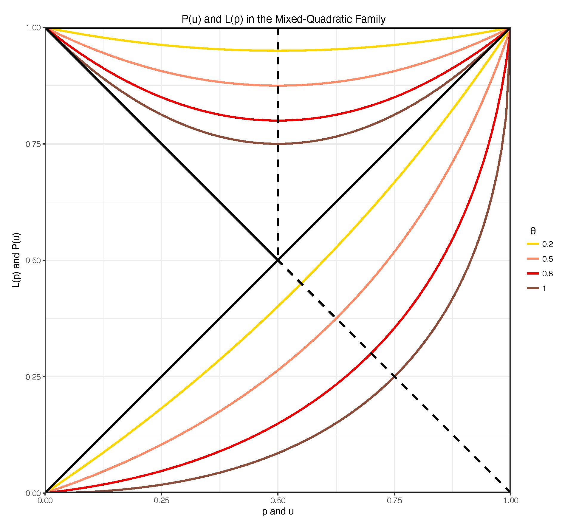
4.2. Tawn’s Mixed-Quadratic Family

Consider the Pickands function

$$P\left(u\right)=\theta u^2-\theta u+1,u,\theta \in [0,1].$$

(9)

This model easily characterizes independence for $\theta =0$, but it cannot deal with full dependence [8]. Moreover, the function $P\left(u\right)$ is symmetric with respect to the vertical line passing through (1/2,0) and (1/2,1), and this implies that the margins of the corresponding copula are exchangeable.

The associated Lorenz curve is obtained as follows. From Equations (8) and (9), we know that

$$K^{-1}\left(u\right)=-\theta u^2+(1+\theta )u$$

(10)

Recalling the properties of $K\left(p\right)$, we easily derive

$$K\left(p\right)={\displaystyle \frac{-\sqrt{{\theta }^2-4\theta p+2\theta +1}+\theta +1}{2\theta }},$$

(11)

and then

$$L\left(p\right)={\displaystyle \frac{-\sqrt{{\theta }^2-4\theta p+2\theta +1}+\theta +1}{\theta }}-p.$$

(12)

Equation (12) is interesting, as we recognize it as the elliptical Lorenz of the inequality studies literature [32]. Up to re-parametrization, we can immediately rewrite Equation (12) as

$$L\left(p\right)={\displaystyle \frac{a-\beta p-\sqrt{a^2+bp+c}}{2}},$$

(13)

with $a={\displaystyle \frac{2(\theta +1)}{\theta }}$, $\beta =2$, $b=-{\displaystyle \frac{16}{\theta }}$, and $c=0$, obtaining the original formulation of [32]. The elliptical Lorenz preserves the symmetry of the original Pickands function, even if symmetry is now with respect to the diagonal of the unit square. In general, simple geometrical considerations guarantee that (a) symmetric Pickands functions correspond to (a) symmetric Lorenz curves, and vice versa. In [30] a sufficient criterion for the symmetry of a Lorenz curve is given, and it can be used to discuss symmetry in the Pickands domain as well.

Figure 6 shows the relation between the Pickands and Lorenz curves in the mixed-quadratic family for different values of the parameter $\theta$.

Since there is a one-to-one correspondence between a given Lorenz curve and a Pickands model, and noting that the elliptical Lorenz is a 4-parameter family of curves, we can conclude that the mixed model for the Pickands defined in Equation (9) is just a restriction of a larger class of models obtainable from the underlying Lorenz family. With this in mind one could ideally increase the flexibility of the 1-parameter mixed model by looking at the entire class of associated 4-parameter Lorenz curves.

4.3. The Marshall–Olkin Case

Let us consider the Marshall–Olkin bivariate copula [3], whose Pickands function, with parameter $\gamma \in [0,1]$, is given by the following equation:

$$P\left(u\right)=1-\gamma +\gamma max(u,1-u),u\in [0,1].$$

This model interpolates between independence ($\gamma =0$) and perfect dependence ($\gamma =1$). We focus on the non-degenerate case $\gamma \in [0,1)$, where inversion is piecewise smooth.

Following our approach, we immediately get

$$K^{-1}\left(u\right)=u+\gamma -\gamma max(u,1-u),$$

which simplifies piecewise. For $u\in [0,0.5]$, one has $max(u,1-u)=1-u$, and

$$K^{-1}\left(u\right)=u+\gamma -\gamma (1-u)=(1+\gamma )u.$$

For $u\in (0.5,1]$, it holds $max(u,1-u)=u$, and

$$K^{-1}\left(u\right)=u+\gamma -\gamma u=(1-\gamma )u+\gamma .$$

We now invert these expressions to recover $K\left(p\right)$. For $p=(1+\gamma )u$, valid when $u\in [0,0.5]$, we obtain

$$K\left(p\right)={\displaystyle \frac{p}{1+\gamma }},\mathrm{for}p\in \left[0,{\displaystyle \frac{1+\gamma }{2}}\right].$$

For $p=(1-\gamma )u+\gamma$, valid when $u\in (0.5,1]$, we obtain

$$K\left(p\right)={\displaystyle \frac{p-\gamma }{1-\gamma }},\mathrm{for}p\in \left({\displaystyle \frac{1+\gamma }{2}},1\right].$$

Finally, recall the identity $K\left(p\right)={\displaystyle \frac{L\left(p\right)+p}{2}}$, which yields $L\left(p\right)=2K\left(p\right)-p$.

Substituting the expressions for $K\left(p\right)$ into this formula we get

$$L\left(p\right)=2\left({\displaystyle \frac{p}{1+\gamma }}\right)-p={\displaystyle \frac{1-\gamma }{1+\gamma }}p$$

for $p\in \left[0,{\displaystyle \frac{1+\gamma }{2}}\right]$. While, for $p\in \left({\displaystyle \frac{1+\gamma }{2}},1\right]$, we find

$$L\left(p\right)=2\left({\displaystyle \frac{p-\gamma }{1-\gamma }}\right)-p={\displaystyle \frac{(1+\gamma )p-2\gamma }{1-\gamma }}.$$

Hence, the Lorenz curve associated with the Marshall–Olkin bivariate copula is

$$L_{MO}\left(p\right)=\left\{\begin{array}{cc}{\displaystyle \frac{1-\gamma }{1+\gamma }}p\hfill & \mathrm{if}p\in \left[0,{\displaystyle \frac{1+\gamma }{2}}\right]\hfill \\ {\displaystyle \frac{(1+\gamma )p-2\gamma }{1-\gamma }}\hfill & \mathrm{if}p\in \left({\displaystyle \frac{1+\gamma }{2}},1\right].\hfill \end{array}\right.$$

Figure 7 shows the behavior of $L_{MO}\left(p\right)$ for some values of $\gamma$.

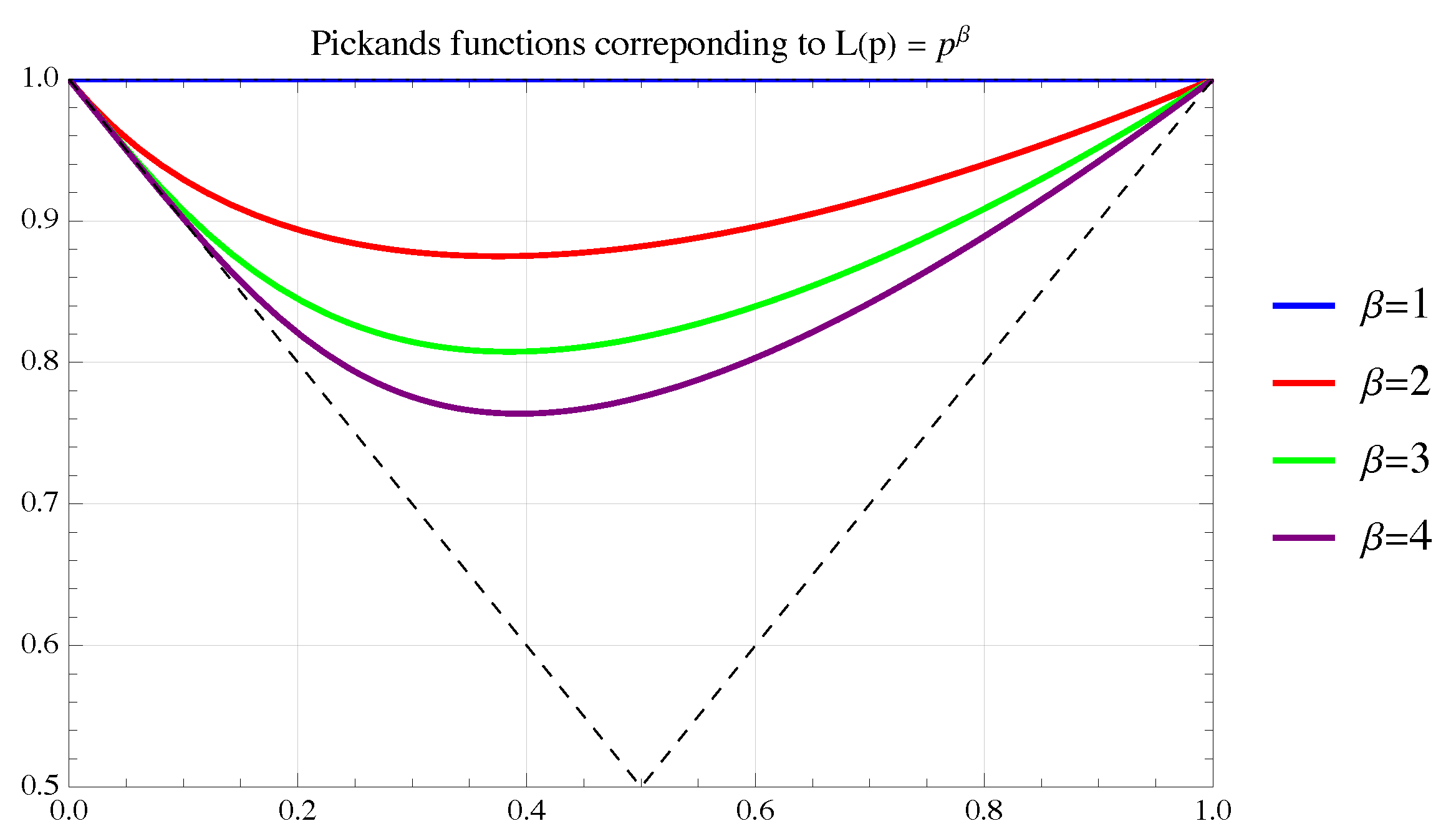
4.4. The Power-Law Lorenz and the Asymmetric Pickands

Consider the Lorenz curve defined by

$$L_{\beta }\left(p\right)=p^{\beta },\beta \ge 1,p\in [0,1].$$

(14)

The corresponding function $K_{\beta }\left(p\right)$, required for the Lorenz-to-Pickands transformation, is explicitly given by

$$K_{\beta }\left(p\right)={\displaystyle \frac{p^{\beta }+p}{2}}.$$

(15)

The inverse $K_{\beta }^{-1}\left(u\right)$ admits closed-form expressions for certain values of $\beta$. For example, for $\beta =1$, we immediately find

$$K_{\beta =1}^{-1}\left(u\right)=u.$$

(16)

For $\beta =2$, one obtains the simple analytical form

$$K_{\beta =2}^{-1}\left(u\right)={\displaystyle \frac{\sqrt{8u+1}-1}{2}}.$$

(17)

For $\beta =3$, things get a little more cumbersome, but the explicit solution is given by

$$K_{\beta =3}^{-1}\left(u\right)=\sqrt[3]{u+\sqrt{u^2+{\displaystyle \frac{1}{27}}}}+\sqrt[3]{u-\sqrt{u^2+{\displaystyle \frac{1}{27}}}}.$$

(18)

Finally, for $\beta =4$, one has

$$K_{\beta =4}^{-1}\left(u\right)={\displaystyle \frac{6^{2/3}}{12}}\left(\sqrt{-A+B}+\sqrt{A-B-{\displaystyle \frac{12}{\sqrt{-A+B}}}}\right),$$

(19)

where

$$R=\sqrt{2048u^3+27},S={(\sqrt{3}R+9)}^{1/3},A={\displaystyle \frac{16·3^{1/3}u}{S}},B=2^{1/3}S,$$

(20)

Applying $P_{\beta }\left(u\right)=1+u-K_{\beta }^{-1}\left(u\right)$ then leads to the desired Pickands functions, which are characterized by an interesting asymmetry—inherited from $L_{\beta }\left(p\right)$—as Figure 8 shows.

For values of $\beta$ other than $1,2,3,4$, solutions typically involve transcendental functions when in closed form, or require numerical methods for evaluation.

Remark 1. 

Asymmetry in the Pickands dependence function is particularly valuable, as it allows for directional differences in the dependence structure, capturing real-world (financial) scenarios more accurately [16,21]. In practical applications, this asymmetry can significantly enhance modeling accuracy, reflecting realistic situations where extreme events in one variable influence another variable differently than vice versa [4,6].

An asymmetric Pickands function, where $P\left(u\right)\ne P(1-u)$, implies that the intensity of tail co-movement is conditional on the source of the extreme shock. The argument u in $P\left(u\right)$ can be interpreted as the relative contribution of the first variable to the severity of the joint extreme event. A symmetric Pickands function, which is minimised at $u_{min}=1/2$, imposes the restriction that tail dependence is strongest when both variables contribute equally to the joint extremes. It assumes the dependence structure is identical regardless of which variable leads the extreme event. An asymmetric Pickands function, with a minimum at $u_{min}\ne 1/2$, models a directional dependence. If $u_{min}>1/2$, the tail dependence is strongest when an extreme event in the first variable is more severe than the corresponding event in the second; the first variable is thus the dominant driver of the joint extreme. If $u_{min}<1/2$, the dependence is strongest when the second variable is the primary driver [4].

This property is crucial for moving beyond overly simplistic assumptions of balanced dependence and capturing the nuanced, often one-sided, nature of financial contagion and risk amplification. A well-known stylized fact is that large negative returns in the stock market (e.g., S&P 500) are typically accompanied by very large spikes in market volatility (e.g., the VIX index). However, the reverse relationship is weaker: a large spike in volatility does not always trigger a stock market crash of proportional magnitude. This implies an asymmetric tail dependence [38].

The relationship between the fiscal health of a government and its domestic banking sector is also known to be asymmetric. An extreme spike in sovereign bond yields (indicating a potential sovereign debt crisis) almost invariably triggers an extreme spike in the CDS spreads of its major banks, as they hold large amounts of government debt. Conversely, a crisis originating at a single bank may have a much weaker impact on the sovereign’s perceived creditworthiness, unless the bank is systemic [39]. Modeling this “doom loop” for stress-testing or pricing contingent credit products requires an asymmetric copula that correctly reflects that the ‘Sovereign Crisis → Bank Crisis’ link is much stronger in the tail than the reverse.

4.5. The Arnold Family

An interesting and flexible Lorenz curve is the one introduced by Arnold [31,37], defined as

$$L_A\left(p\right)=F\left(F^{-1}\left(p\right)-c\right),$$

(21)

where F is the cumulative distribution function (CDF) of a unimodal random variable X, and $c>0$ is a parameter (one could also set $c=0$, but then trivially $L_A\left(p\right)=p$). Such a Lorenz has been introduced as a generalization of the well-known lognormal Lorenz [30], known as

$$L\left(p\right)=\mathrm{\Phi }\left({\varphi }^{-1}\left(p\right)-c\right),$$

(22)

where $\mathrm{\Phi }$ is the CDF of a standard Gaussian random variable.

While Equation (22) does not allow for the discovery of a closed form for the corresponding $P\left(u\right)$—and we refer to Section 5 for more details—one can look for a F that allows for it. We here discuss two interesting cases.

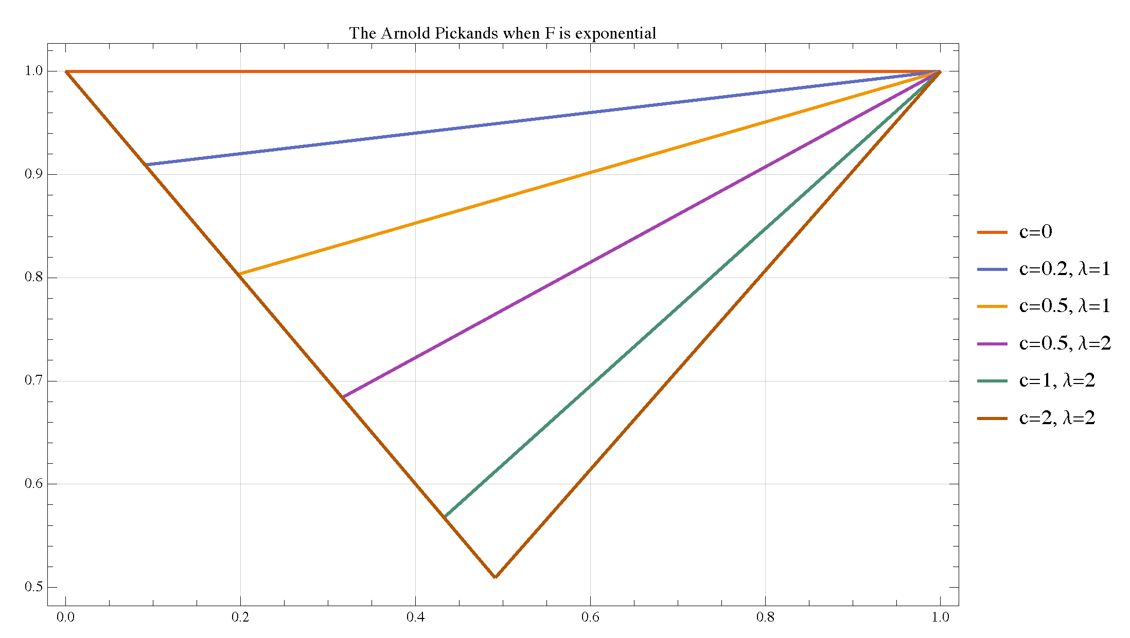
4.5.1. F Is Exponential

Let F be the exponential CDF with a generic intensity parameter $\lambda >0$. Clearly,

$$F\left(x\right)=1-e^{-\lambda x},$$

for $x\ge 0$, and $F\left(x\right)=0$ for $x<0$.

The inverse of F, for $p\in [0,1)$, is

$$F^{-1}\left(p\right)=-{\displaystyle \frac{1}{\lambda }}ln(1-p).$$

(23)

Next, we substitute $F^{-1}\left(p\right)$ into Arnold’s definition of $L\left(p\right)$ as per Equation (21). The argument for F becomes $A\left(p\right)=F^{-1}\left(p\right)-c=-{\displaystyle \frac{1}{\lambda }}ln(1-p)-c$. Due to the piecewise nature of the exponential CDF, we must consider the sign of $A\left(p\right)$. One immediately sees that

$$A\left(p\right)<0\iff p<1-e^{-\lambda c}.$$

Let $p_0=1-e^{-\lambda c}$. Since $\lambda >0$ and $c>0$, we have $p_0\in (0,1)$.

Thus, $L\left(p\right)$ is a piecewise function. If $0\le p<p_0$, we have $L\left(p\right)=F\left(A\right(p\left)\right)=0$. If $p_0\le p\le 1$, we get

$$L\left(p\right)=1-e^{\lambda c}+p{e}^{\lambda c}.$$

The full Lorenz curve is therefore

$$L\left(p\right)=\left\{\begin{array}{cc}0\hfill & \mathrm{if}0\le p<1-e^{-\lambda c}\hfill \\ 1-e^{\lambda c}+p{e}^{\lambda c}\hfill & \mathrm{if}1-e^{-\lambda c}\le p\le 1\hfill \end{array}\right.,$$

which represents an interesting case of the Lorenz curve, in which a proportion of the population is allowed to have a null income or wealth.

Following our procedure to map the Lorenz curve to the Pickands dependence function, we then obtain

$$K\left(p\right)=\left\{\begin{array}{cc}{\displaystyle \frac{p}{2}}\hfill & \mathrm{if}0\le p<1-e^{-\lambda c}\hfill \\ {\displaystyle \frac{1-e^{\lambda c}+p(1+e^{\lambda c})}{2}}\hfill & \mathrm{if}1-e^{-\lambda c}\le p\le 1\hfill \end{array}\right.,$$

and

$$K^{-1}\left(u\right)=\left\{\begin{array}{cc}2u\hfill & \mathrm{if}0\le u<{\displaystyle \frac{1-e^{-\lambda c}}{2}}\hfill \\ {\displaystyle \frac{2u-1+e^{\lambda c}}{1+e^{\lambda c}}}\hfill & \mathrm{if}{\displaystyle \frac{1-e^{-\lambda c}}{2}}\le u\le 1\hfill \end{array}\right..$$

Exploiting $P\left(u\right)=1+u-K^{-1}\left(u\right)$, we finally obtain the piecewise linear Pickands function

$$P_{Exp}\left(u\right)=\left\{\begin{array}{cc}1-u\hfill & \mathrm{if}0\le u<{\displaystyle \frac{1-e^{-\lambda c}}{2}}\hfill \\ {\displaystyle \frac{2-u+u{e}^{\lambda c}}{1+e^{\lambda c}}}\hfill & \mathrm{if}{\displaystyle \frac{1-e^{-\lambda c}}{2}}\le u\le 1\hfill \end{array}\right.,$$

which is shown in Figure 9 for different values of c and $\lambda$. For $c=0$, no matter $\lambda$, $P_{Exp}\left(u\right)$ corresponds to the case of tail independence. For $c>0$, the larger the value of c, the stronger the dependence, with $\lambda$ governing the asymmetry on the left-hand side (the minimum of $P_{Exp}\left(u\right)$ will always have $u\in [0,1/2]$). For a large enough value of c and $\lambda$, the full tail dependence case can be recovered, and the minimum point becomes $(1/2,1/2)$.

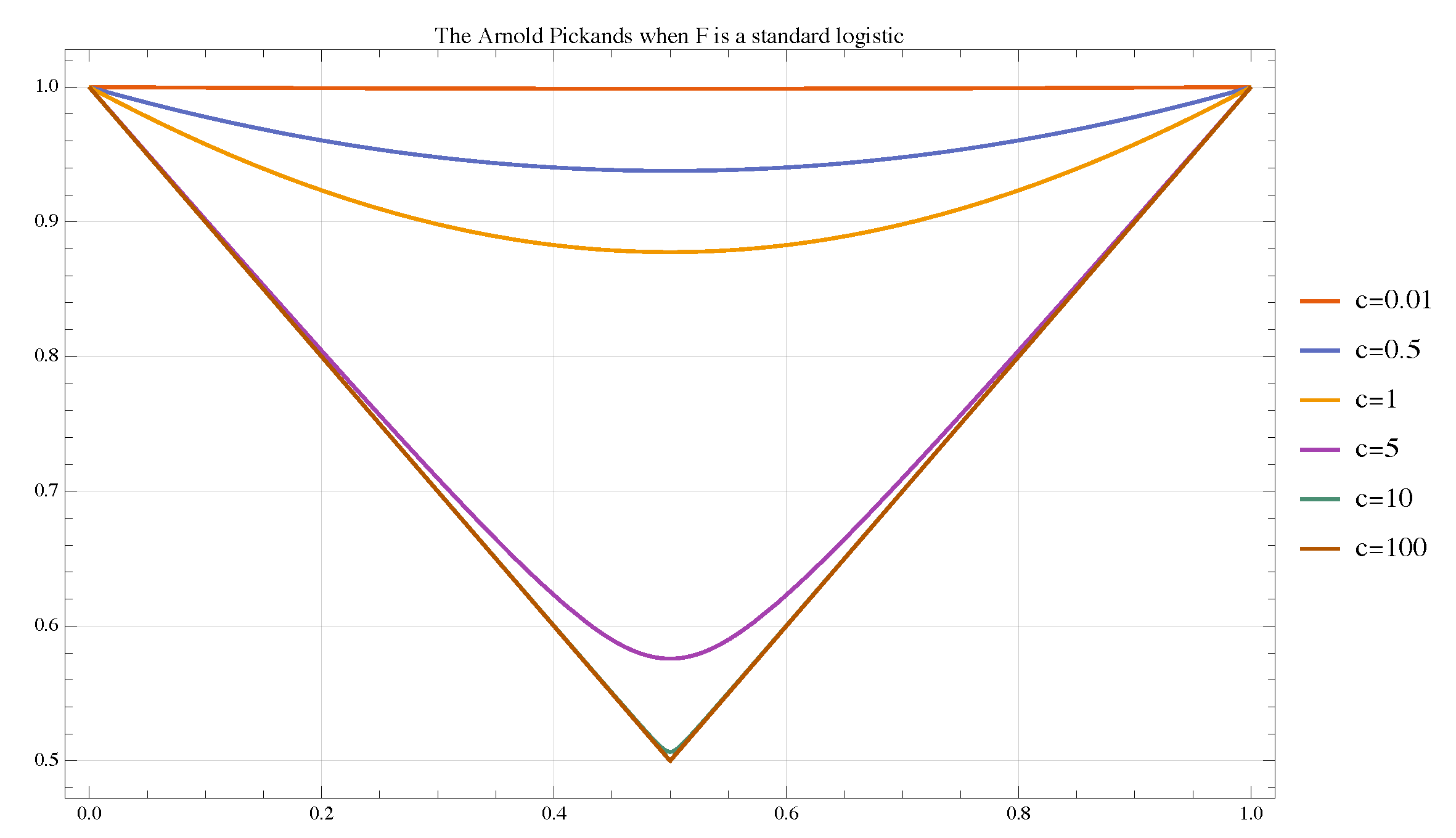
4.5.2. F Is a Standard Logistic

Let F be a standard Logistic CDF, that is,

$$F\left(x\right)={\displaystyle \frac{1}{1+e^{-x}}}.$$

Applying Arnold’s definition as per Equation (21), the corresponding Lorenz becomes

$$L\left(p\right)={\displaystyle \frac{p}{p+(1-p)e^c}}.$$

This leads to

$$K\left(p\right)={\displaystyle \frac{1}{2}}\left({\displaystyle \frac{p}{p+(1-p)e^c}}+p\right)={\displaystyle \frac{p+p^2+p{e}^c-p^2{e}^c}{2(p+e^c-p{e}^c)}}.$$

To find $K^{-1}\left(u\right)$, we set $u=K\left(p\right)$ and solve for p. This leads to the quadratic equation:

$$p^2(1-e^c)+p(1+e^c)(1-2u)-2u{e}^c=0.$$

This is a quadratic equation of the form $A{p}^2+Bp+C=0$, where $A=1-e^c$, $B=(1+e^c)(1-2u)$, and $C=-2u{e}^c$. The solution for $p=K^{-1}\left(u\right)$ is, therefore, of the form $p={\displaystyle \frac{-B\pm \sqrt{B^2-4AC}}{2A}}$.

For $u\in [0,1]$, we select the appropriate sign for the square root to obtain the desired $p\in [0,1]$. Thus, $K^{-1}\left(u\right)$ is given by

$$K^{-1}\left(u\right)={\displaystyle \frac{-(1+e^c)(1-2u)+\sqrt{{(1+e^c)}^2{(1-2u)}^2+8u{e}^c(1-e^c)}}{2(1-e^c)}},$$

and the Pickands function $P_{Logi}\left(u\right)$ follows. Figure 10 shows that $P_{Logi}\left(u\right)$ is a symmetric Pickands, whose shape is governed by the parameter c of the Arnold construction. For $c\to 0$, it approaches the tail independence case, while for $c\to +\infty$ it moves towards perfect tail dependence.

4.6. Other Cases

Several other cases exist in which both the Lorenz and Pickands dependence functions admit analytical closed-form solutions. Typically, these special cases correspond to particular parameterizations of well-known Lorenz families.

An example is represented by the Lorenz curve derived from the classical Type I Pareto distribution [30], which is given by

$$L_{\alpha }\left(p\right)=1-{(1-p)}^{1-1/\alpha },\alpha >1.$$

(24)

While this Lorenz curve generally requires numerical inversion to obtain the corresponding Pickands function, it admits closed-form results in specific cases.

For $\alpha =1$, the Lorenz curve simplifies to the perfect inequality line, yielding $P_{\alpha =1}\left(u\right)=max(u,1-u)$, i.e., perfect tail dependence.

For $\alpha =2$, the Lorenz curve becomes

$$L_{\alpha =2}\left(p\right)=1-{(1-p)}^{1/2}.$$

(25)

then

$$K_{\alpha =2}\left(p\right)={\displaystyle \frac{1-{(1-p)}^{1/2}+p}{2}},$$

(26)

and

$$K_{\alpha =2}^{-1}\left(u\right)={\displaystyle \frac{4u-3+\sqrt{9-8u}}{2}},$$

(27)

so that the asymmetric $P_{\alpha =2}\left(u\right)$ follows, reaching its minimum $7/8$ on the right end-side of the Pickands triangle, in $u=5/8$.

5. When $\mathit{K}\left(\mathit{p}\right)$ Is Not Invertible

While several Lorenz–Pickands pairs admit closed-form expressions, many important and practically relevant cases do not. In these situations, the inversion of the function $K\left(p\right)$ cannot be performed analytically. Nevertheless, the transformation remains fully constructive because the numerical inversion of $K\left(p\right)$ is particularly robust.

For any target $u\in [0,1]$, the root of the monotonic function $K\left(p\right)-u=0$ is sought on the bounded interval $[0,1]$, which guarantees convergence for standard bracketing algorithms. Furthermore, the analytical derivative $K^{\prime }\left(p\right)={\displaystyle \frac{1}{2}}(L^{\prime }\left(p\right)+1)$ is strictly positive, allowing for the use of rapidly converging gradient-based solvers like the Newton–Raphson method. Given these properties, the problem is numerically manageable for standard scientific libraries, such as the uniroot function in R or FindRoot in Mathematica, which can perform this step with high precision and negligible cost. From an applied viewpoint, at present, the critical challenge is therefore not the numerical transformation, but the quality of the initial data used to obtain the nonparametric estimate of the dependence structure [9], as we also note in Section 9.

The numerical route enables the construction of Pickands functions from Lorenz curves, and vice versa, that would otherwise be inaccessible. In particular, it allows us to treat cases where the Lorenz curve involves logarithmic, exponential, or non-algebraic terms. Let us consider a couple of examples.

5.1. The Lognormal Lorenz

A Lorenz curve derived from a lognormally distributed random variable is given by the following equation:

$$L_{\sigma }\left(p\right)=\mathrm{\Phi }\left({\mathrm{\Phi }}^{-1}\left(p\right)-{\sigma }^2\right),$$

(28)

where $\mathrm{\Phi }$ and ${\mathrm{\Phi }}^{-1}$ are the standard normal CDF and quantile function, respectively. We have seen that it represent a special case of the more general construction by Arnold, as given in Equation (21).

The associated function $K\left(p\right)={\displaystyle \frac{L\left(p\right)+p}{2}}$ is well defined and strictly increasing, but its inverse $K^{-1}\left(u\right)$ cannot be expressed in closed form. Nevertheless, numerical inversion of $K\left(p\right)$ allows one to find the corresponding Pickands, as shown in Figure 11. Since the lognormal Lorenz is known to be symmetric with respect to the antidiagonal of the unit square, the corresponding Pickands is symmetric with respect to $u=1/2$.

Remark 2. 

Equation (28) is of particular interest in financial and actuarial mathematics. Besides being a Lorenz curve, it is also the distortion function [40], known as the Wang transform [41], that governs the change in measure between the market measure $\mathbb{P}$ and the risk neutral measure $\mathbb{Q}$ in the standard Black–Scholes framework. Moreover, in the theory of copulas, it has been used as a generator to define a class of non-strict Archimedean copulas characterized by asymptotic tail dependence, which can find applicability in operational risk management and the modeling of cat bonds [15].

5.2. Hüsler–Reiss Copula

The Hüsler–Reiss copula [42] is a famous extreme-value model that arises as the limit of component-wise maxima of Gaussian vectors. In its original definition, its symmetric Pickands dependence function is given by the following equation:

$$P_{\lambda }\left(u\right)=u\mathrm{\Phi }\left({\displaystyle \frac{1}{\lambda }}+{\displaystyle \frac{\lambda }{2}}log\left({\displaystyle \frac{1-u}{u}}\right)\right)+(1-u)\mathrm{\Phi }\left({\displaystyle \frac{1}{\lambda }}+{\displaystyle \frac{\lambda }{2}}log\left({\displaystyle \frac{u}{1-u}}\right)\right),$$

(29)

where $\mathrm{\Phi }$ is once again the standard normal CDF, and $\lambda >0$. While the expression is explicit, it is not in a form that can be easily inverted to recover a corresponding symmetric Lorenz curve in closed form. However, this is a task that can be easily conducted numerically, which is also true for the more recent asymmetric versions [43].

6. Indices of (In)Equality and (In)Dependence

We have established a connection between $P\left(u\right)$ and a unique $L\left(p\right)$ associated with it. As this link bridges extreme value theory and the study of inequality, it allows us to introduce established inequality indices not merely as analogues, but as direct summary measures for the concentration, structure, and asymmetry of bivariate tail dependence.

This approach offers advantages over traditional scalar indices of tail dependence. For example, the widely used upper tail dependence coefficient [4], ${\lambda }_U=2-2P(1/2)$, quantifies the probability of joint extremes assuming a degree of symmetry (by focusing on $u=1/2$). While ${\lambda }_U$ offers a single useful value, it condenses the entire tail dependence structure into one point, potentially overlooking crucial aspects if the dependence is asymmetric. In contrast, inequality indices derived from the full $L\left(p\right)$ provide a more holistic understanding.

From the rich toolkit of inequality analysis, we select two prominent indices, the Gini coefficient and the Pietra index [13,30], to apply to $L\left(p\right)$, thereby reinterpreting them as measures of tail dependence.

The Gini coefficient is widely used to measure inequality. Geometrically, it can be defined as twice the area between the Lorenz of perfect equality $L_{PE}\left(p\right)$ and $L\left(p\right)$, or

$$G=1-2{\int }_0^{1}L\left(p\right)\mathrm{d}p.$$

Clearly, in our setting $G=0$ indicates tail independence, because it would imply $L\left(p\right)=p$, and, therefore, $P\left(u\right)=1$ for all $u\in [0,1]$. On the opposite side, $G=1$ corresponds to perfect inequality and thus perfect tail dependence. All other values of G from 0 to 1 represent increasing tail dependence.

The Pietra index measures the maximum vertical distance between the line of perfect equality and a Lorenz curve $L\left(p\right)$, quantifying the maximum deviation from perfect equality, that is,

$$H=\underset{p\in [0,1]}{max}(p-L\left(p\right)).$$

It is easy to see that $H=0$ indicates tail independence, while $H=1$ indicates perfect tail dependence. However, by going back to Section 3, we can get additional insight, which makes H particularly interesting when applied to tail dependence.

Let $P_{min}={min}_{u\in [0,1]}P\left(u\right)$ be the minimum value of the Pickands function. By looking at Figure 5, we immediately find that $P_{min}=1-{max}_u\overline{D}\left(u\right)$ in the Gini coordinate system. This tells us that

$$H=2(1-P_{min}).$$

(30)

Calculating the Pietra index thus implicitly provides information on the (absolute) minimum of the Pickands function $P_{min}$ as well. This ensures H captures the true peak intensity of dependence, regardless of where it occurs.

Naturally, $P_{min}$ can also be used to verify the symmetry of both the $P\left(u\right)$ and $L\left(p\right)$. Let $u_{min}\in [0,1]$ be the value where $P\left(u\right)$ achieves its minimum $P_{min}$. We can define the asymmetry index

$$S=2u_{min}-1\in [-1,1].$$

The value $S_P=0$ indicates a symmetric Pickands (and Lorenz) function where the strongest dependence (minimum $P\left(u\right)$ value) occurs at $u=1/2$. A non-zero S signifies asymmetry, with its sign indicating the direction of the skew in the dependence structure.

6.1. A Few Examples

Let us consider a few examples for the use of G, H, and S, leaving to the interesting reader the derivations for the other cases.

In the Tawn’s mixed family, the Pickands function is symmetric and equal to $P\left(u\right)=\theta u^2-\theta u+1$, $\theta \in [0,1]$. It follows that $u_{min}={\displaystyle \frac{1}{2}}$, and $S=0$. Consequently, $P_{min}=P\left({\displaystyle \frac{1}{2}}\right)=1-{\displaystyle \frac{\theta }{4}}$, $H={\displaystyle \frac{\theta }{2}}$ (coinciding with ${\lambda }_U$), and $G={\displaystyle \frac{\theta }{3}}.$ For this symmetric family, dependence increases with $\theta$, as expected.

In the Marshall–Olkin copula, another symmetric case, $P\left(u\right)=1-\gamma +\gamma max(u,1-u)$, so that $S=0$, and $G=H=\gamma$.

Let us now consider the power law case of Section 4.4, where $L\left(p\right)=p^{\beta }$, and $P\left(u\right)$ can be obtained in closed-form or numerically depending on the value of $\beta \ge 1$. The Gini index is $G=1-{\displaystyle \frac{2}{\beta +1}}$, and dependence increases with $\beta$. The Pietra index is $H=0$ for $\beta =1$, and $H=(\beta -1){\beta }^{-(1+{\displaystyle \frac{1}{\beta -1}})}$ when $\beta >1$. From Equation (30), we get that $P_{min}=1-{\displaystyle \frac{1}{2}}H$, so that we do not need to optimize $P\left(u\right)$ to obtain it. The value $u_{min}$ will be the one corresponding to $P_{min}$, and S follows immediately.

Finally, let

$$L\left(p\right)=\mathrm{\Phi }\left({\mathrm{\Phi }}^{-1}\left(p\right)-\sigma \right),p\in [0,1],$$

be the symmetric Lorenz curve generated by a lognormal random variable of parameters $\mu \in \mathbb{R}$ and $\sigma >0$ (note that $\mu$ plays no role in the Lorenz curve). The Gini coefficient is

$$G=2\mathrm{\Phi }\left(\sigma /\sqrt{2}\right)-1,$$

while the Pietra index equals

$$H=2\mathrm{\Phi }\left(\sigma /2\right)-1.$$

Both indices are strictly increasing functions of $\sigma$.

Even if the corresponding Pickands needs to be found numerically, as discussed in Section 5, both G and H can be used to evaluate the dependence structure it induces. Further, we can easily derive $P_{min}=3/2-\left(\sigma /2\right)$, and ${\lambda }_U$ also follows because of symmetry.

6.2. The Risk Management Perspective

In the Pickands–Lorenz framework, the traditional economic concepts of inequality and concentration are repurposed to describe the structure of tail dependence. The core translation is simple: the “inequality of a wealth distribution” becomes the “concentration of joint tail risk”. A society where wealth is highly concentrated in a few hands is analogous to a system where tail risk is highly concentrated, meaning extreme events have a strong tendency to occur together under specific, identifiable conditions. This analogy allows us to imbue classical inequality indices with new, practical meaning for risk management, as already partially observed in [44].

The Gini coefficient measures the total area between the line of perfect equality ($L_{PE}\left(p\right)=p$) and the Lorenz curve $L\left(p\right)$. In our context, it serves as a holistic, scalar measure of the overall concentration of tail dependence across all possible scenarios. In a sense, the Gini coefficient answers the question “How prevalent is tail risk in my system on average?” It is therefore a single number that summarizes the general propensity for joint extremes, much like a credit score summarizes overall creditworthiness.

A low Gini coefficient (near 0) corresponds to a Lorenz curve close to the equality line. This implies that the “risk contribution” is diffuse, and there is no strong, systematic tendency for joint extremes to occur. A high Gini coefficient (near 1) signifies a highly bowed Lorenz curve. This reflects a strong concentration of tail risk, where extreme, impactful events are highly likely to cluster together. A rising Gini for a couple of assets would signal an increasing vulnerability to joint crashes and a general erosion of diversification benefits in the tail.

We know that the Pietra index measures the maximum vertical distance between the line of perfect equality and the Lorenz curve. Its importance is clarified by its direct relationship to the Pickands function, as per Equation (30), i.e., $H=2(1-P_{min})$. This identity makes its interpretation in risk management clear: the Pietra index answers the question “What is the single most dangerous scenario for my portfolio in terms of dependence?” Since $P_{min}$ represents the point of strongest tail dependence, the Pietra index directly quantifies this peak intensity of risk. While the Gini gives an average measure of dependence, the Pietra index isolates the single biggest vulnerability. A high Pietra index tells a risk manager that there exists a specific, identifiable scenario under which diversification benefits will most severely break down. It provides a measure of the magnitude of the worst-case dependence, which is crucial for setting risk limits and capital buffers.

The asymmetry index, S, is derived from the location ($u_{min}$) of the minimum of the Pickands function. It does not measure the level of dependence, but rather diagnoses its nature. If $S=0$ ($u_{min}=1/2$), the dependence structure is symmetric. The highest risk of a joint crash occurs when both risk factors contribute equally. This suggests a balanced co-movement, like that between two highly integrated stock markets (see, e.g., Section 9). If $S\ne 0$, the dependence is asymmetric, indicating a “leader–follower” relationship in the tails, as already observed in Section 4.4. For instance, if $S>0$ ($u_{min}>1/2$), the greatest tail risk occurs when the first asset is the dominant driver of the joint event.

The asymmetry index is thus a diagnostic tool for identifying the source of contagion. It tells a risk manager whether to worry about general, systemic co-movement ($S\approx 0$) or a specific, directional vulnerability where one part of the portfolio is much more likely to infect another ($S\ne 0$). This knowledge is invaluable for designing targeted hedging strategies and more realistic stress tests.

Together, these three indices provide a comprehensive dashboard for tail risk: Gini measures its overall prevalence, Pietra quantifies its peak intensity, and the asymmetry index identifies its primary driver.

6.3. Other Inequality Measures

Beyond the Gini and Pietra indices, our framework allows for the application of numerous other inequality measures to $L\left(p\right)$ and $P\left(u\right)$, each offering different sensitivities and theoretical insights. For instance, the Theil Index, rooted in entropy theory, or the Atkinson Index, which incorporates an inequality aversion parameter, could be adapted to provide further nuanced perspectives on the structure of tail dependence [13,30,31]. The choice of an index would depend on the specific aspect of “dependence concentration” or “extremal risk inequality” that one aims to highlight.

7. A Novel View of the $\mathit{M}$ Measure for the Pickands Dependence Function

The connection between $P\left(u\right)$ and $L\left(p\right)$ also allows for an alternative measure-theoretic view of the Pickands dependence function. In fact, $P\left(u\right)$ can be expressed via a famous integral representation [6], namely

$$P\left(u\right)=1-u+{\int }_0^{u}M\left(x\right)dx,$$

(31)

where $M\left(x\right):=\nu [0,x]$, and $\nu$ is an arbitrary measure on $[0,1]$, with total mass $\nu [0,1]=2$, and expectation $\mathbb{E}\left(\nu \right)=1$.

While this representation provides a theoretically appealing link between the Pickands dependence function and a measure $\nu$, a significant limitation has persisted in the literature: no constructive approach to explicitly determine $\nu$ has been provided. Instead, $\nu$ has remained an abstract entity, introduced as a formal object satisfying the given constraints. A data-driven estimator for M is outlined in [6]: one first estimates P and then recovers M by numerical differentiation [7,8]. While statistically useful, this route offers M only implicitly and does not shed light on its analytic structure. This gap has hindered both the practical applicability of the integral representation of Equation (31) and its theoretical utility in generating new parametric families of Pickands functions.

The Lorenz curve approach proposed here resolves this issue by establishing a direct and explicit construction of $\nu$ and M. By exploiting the one-to-one correspondence between Lorenz curves and Pickands functions, we can effectively transform the problem of identifying the measure $\nu$ into one of characterizing the Lorenz curve and its associated $K\left(p\right)$ function.

Specifically, by combining Equations (8) and (31), we obtain the following representation of the measure $M\left(x\right)$ in terms of the inverse function $K^{-1}\left(u\right)$:

$$K^{-1}\left(u\right)=2u-{\int }_0^{u}M\left(x\right)dx,$$

(32)

which can alternatively be expressed as follows:

$${\int }_0^{u}M\left(x\right)dx=2u-K^{-1}\left(u\right).$$

(33)

Therefore, by specifying a Lorenz curve $L\left(p\right)$, or even the distribution function $F\left(x\right)$ of a positive random variable X with a finite mean, we can represent the measure generating function M and its integral.

By differentiating Equation (32) with respect to u, and by exploiting the implicit function theorem to find the derivative of $K^{-1}\left(u\right)$, we can notice that

$$M\left(u\right)=2-{\displaystyle \frac{1}{K^{\prime }\left(K^{-1}\left(u\right)\right)}},$$

(34)

which can also be written as

$$M\left(u\right)=2-{\displaystyle \frac{2}{\frac{Q\left(K^{-1}\left(u\right)\right)}{{\mu }_X}+1}},$$

(35)

for $u\in [0,1]$, and where $Q(·)$ is the quantile function of the random variable X of which $L\left(p\right)$ is the Lorenz curve.

8. The Lorenz Representation of Extreme-Value Copulas

The framework developed in the preceding sections, linking $P\left(u\right)$ to $L\left(p\right)$ via the intermediary function $K\left(p\right)$, opens a new avenue for characterizing tail dependence. Beyond generating parametric families of Pickands functions, this connection allows us to directly construct bivariate extreme-value copulas from the ground up, starting from a given Lorenz curve.

Recall that a bivariate extreme-value copula $C(y_1,y_2)$, with uniform margins $y_1,y_2\in [0,1]$, can be expressed using its Pickands dependence function $P\left(u\right)$ as follows [4]:

$$C(y_1,y_2)=exp\left(-(-log{y}_1-log{y}_2)P\left({\displaystyle \frac{-log{y}_1}{-log{y}_1-log{y}_2}}\right)\right).$$

(36)

The argument $u={\displaystyle \frac{-log{y}_1}{-log{y}_1-log{y}_2}}$ maps the transformed marginals onto the domain $[0,1]$ of $P\left(u\right)$. Given our established relationship $P\left(u\right)=1+u-K^{-1}\left(u\right)$, we can now state the following proposition.

Proposition 2. 

Let $L\left(p\right)$ be a valid Lorenz curve for $p\in [0,1]$. Define $K\left(p\right)={\displaystyle \frac{1}{2}}(L\left(p\right)+p)$, and assume it is invertible, so that $K^{-1}\left(u\right)$ is well-defined, unique, concave, and strictly increasing for $u\in [0,1]$. Then, the unique bivariate extreme-value copula $C_L(y_1,y_2)$ corresponding to the Lorenz curve $L\left(p\right)$ is given by the following equation:

$$C_L(y_1,y_2)=exp\left(2log{y}_1+log{y}_2+(-log{y}_1-log{y}_2)K^{-1}\left({\displaystyle \frac{-log{y}_1}{-log{y}_1-log{y}_2}}\right)\right),$$

(37)

for $y_1,y_2\in (0,1]$. Alternatively, letting $z_1=-log{y}_1$ and $z_2=-log{y}_2$, the copula can be written as follows:

$$C_L(e^{-z_1},e^{-z_2})=exp\left(-2z_1-z_2+(z_1+z_2)K^{-1}\left({\displaystyle \frac{z_1}{z_1+z_2}}\right)\right),$$

(38)

for $z_1,z_2>0$.

Proof. 

The standard representation of a bivariate extreme-value copula is given by Equation (36). Using the relationship $P\left(u\right)=1+u-K^{-1}\left(u\right)$, where $u={\displaystyle \frac{-log{y}_1}{-log{y}_1-log{y}_2}}$, we substitute this into the exponent of Equation (36), and we get

$$\begin{array}{cc}\hfill & -(-log{y}_1-log{y}_2)P\left({\displaystyle \frac{-log{y}_1}{-log{y}_1-log{y}_2}}\right)\hfill \\ \hfill & =-(-log{y}_1-log{y}_2)\left[1+{\displaystyle \frac{-log{y}_1}{-log{y}_1-log{y}_2}}-K^{-1}\left({\displaystyle \frac{-log{y}_1}{-log{y}_1-log{y}_2}}\right)\right]\hfill \\ \hfill & =(log{y}_1+log{y}_2)-(-log{y}_1)+(-log{y}_1-log{y}_2)K^{-1}\left({\displaystyle \frac{-log{y}_1}{-log{y}_1-log{y}_2}}\right)\hfill \\ \hfill & =2log{y}_1+log{y}_2+(-log{y}_1-log{y}_2)K^{-1}\left({\displaystyle \frac{-log{y}_1}{-log{y}_1-log{y}_2}}\right).\hfill \end{array}$$

Substituting this back into the exponential function yields Equation (37). Note that this exponent can also be written as $-(x_1+x_2)P\left(u_0\right)$, where $u_0=x_1/(x_1+x_2)$, by substituting $P\left(u_0\right)=1+u_0-K^{-1}\left(u_0\right)$ into $-(x_1+x_2)P\left(u_0\right)$ and simplifying, which confirms consistency with the standard form involving $P\left(u_0\right)$. The transformation to $x_1=-log{y}_1$ and $x_2=-log{y}_2$ directly yields Equation (38).    □

Proposition 2 provides an explicit bridge from the domain of inequality measurement (represented by $L\left(p\right)$) to the direct specification of extreme-value dependence structures. Any valid Lorenz curve, through the $K\left(p\right)$ transformation and its inverse, now uniquely defines a bivariate extreme-value copula. The adequate transformation of margins is inherently handled by the standard formulation of extreme-value copulas.

This result not only enriches the theoretical understanding of the interplay between these two fields but also provides a novel practical mechanism: one can now select a Lorenz curve based on economic or inequality criteria and immediately derive the corresponding tail behavior model for bivariate extremes.

Examples

We now illustrate Proposition 2 with some examples previously discussed in the context of Pickands and Lorenz functions. Let $z_1=-log{y}_1$, $z_2=-log{y}_2$, and $u_0={\displaystyle \frac{z_1}{z_1+z_2}}$. Then $C(y_1,y_2)=exp\left(-(z_1+z_2)P\left(u_0\right)\right)$, where $P\left(u_0\right)=1+u_0-K^{-1}\left(u_0\right)$.

For the perfect equality Lorenz curve, $L\left(p\right)=p$ for all $p\in [0,1]$, we get $K^{-1}\left(u_0\right)=u_0$. Therefore substituting into the extreme-value copula

$$C(y_1,y_2)=exp(-(z_1+z_2)·1)=exp(-z_1-z_2)=e^{-z_1}{e}^{-z_2}=y_1{y}_2.$$

This is the independence copula, $C(y_1,y_2)=y_1{y}_2$, correctly reflecting that perfect equality in this framework corresponds to tail independence.

For the perfect inequality Lorenz curve, $L\left(p\right)=0$ for $p\in [0,1)$ and $L\left(1\right)=1$, we have $K^{-1}\left(u_0\right)=1+u_0-max(u_0,1-u_0)$. This implies the following: (1) if $u_0\in [0,1/2]$, then $K^{-1}\left(u_0\right)=1+u_0-(1-u_0)=2u_0$; (2) if $u_0\in (1/2,1]$, then $K^{-1}\left(u_0\right)=1+u_0-u_0=1$.

It follows that

$$C(y_1,y_2)=exp\left(-(z_1+z_2)max(u_0,1-u_0)\right).$$

Since $u_0={\displaystyle \frac{z_1}{z_1+z_2}}$ and $1-u_0={\displaystyle \frac{z_2}{z_1+z_2}}$:

$$(z_1+z_2)max\left({\displaystyle \frac{z_1}{z_1+z_2}},{\displaystyle \frac{z_2}{z_1+z_2}}\right)=max(z_1,z_2).$$

thus,

$$C(y_1,y_2)=exp(-max(z_1,z_2))=exp(min(-z_1,-z_2))=min(e^{-z_1},e^{-z_2})=min(y_1,y_2).$$

This is the Fréchet–Hoeffding upper bound, or comonotonicity copula, representing perfect positive dependence.

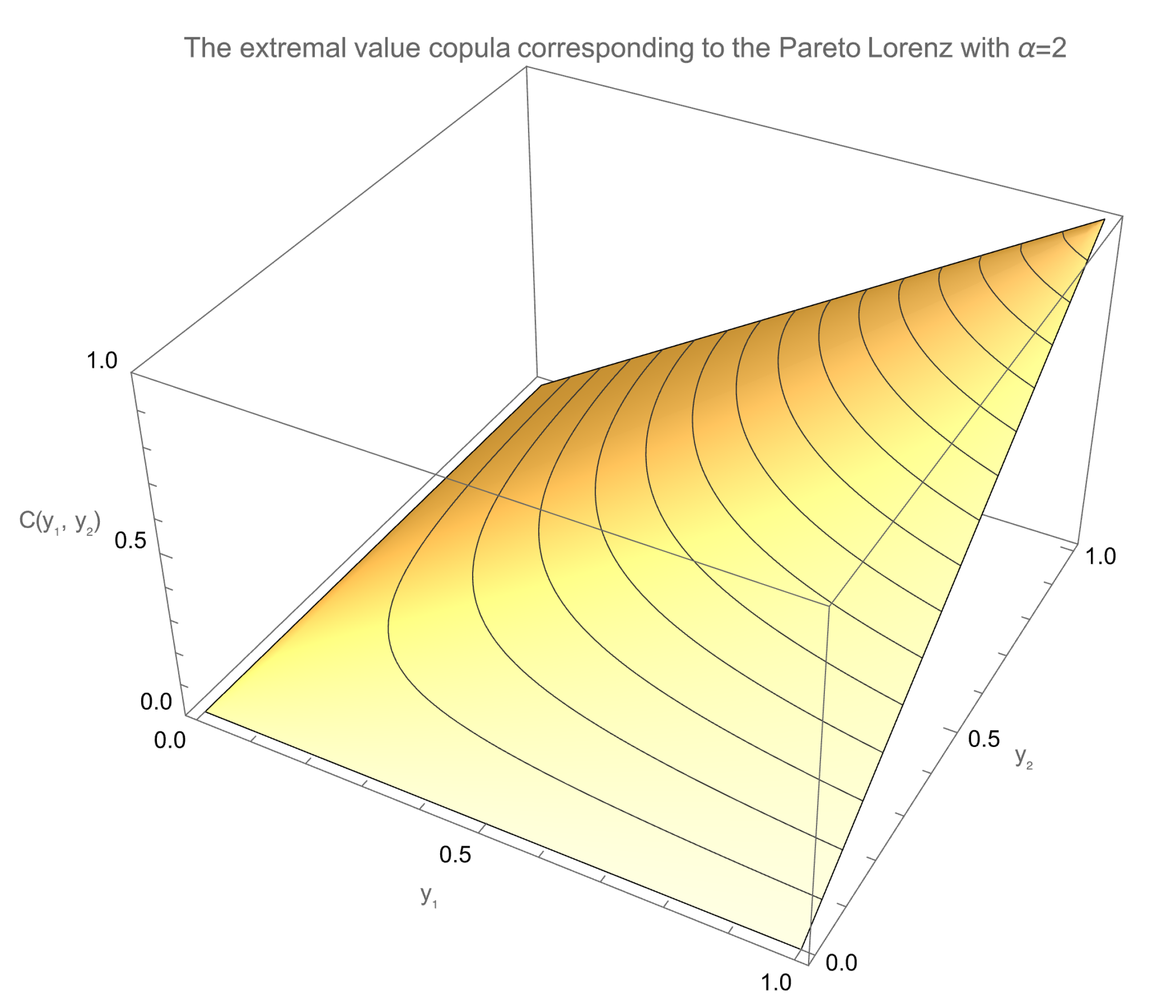
Now, let us consider the simple Pareto case of Section 4.6, Equation (25), so that $L\left(p\right)=1-{(1-p)}^{1/2}$. We notice that $K^{-1}\left(u_0\right)={\displaystyle \frac{4u_0-3+\sqrt{9-8u_0}}{2}}$. From this we get the new copula

$$C(y_1,y_2)=exp\left(-(z_1+z_2)\left[{\displaystyle \frac{5-2\left(\frac{z_1}{z_1+z_2}\right)-\sqrt{9-8\left(\frac{z_1}{z_1+z_2}\right)}}{2}}\right]\right),$$

which is shown in Figure 12. Or, equivalently, by substituting $u_0={\displaystyle \frac{-log{y}_1}{-log{y}_1-log{y}_2}}$,

$$C(y_1,y_2)=exp\left(-(-log{y}_1-log{y}_2)\left[{\displaystyle \frac{5-2u_0-\sqrt{9-8u_0}}{2}}\right]\right).$$

9. A Simple Application: DAX vs. SMI

To illustrate the practical utility of the Lorenz–Pickands framework, we analyze the upper tail dependence between two major, highly integrated European stock markets: the German stock index DAX (GDAXI) and the Swiss Market Index (SMI). We use daily data spanning from 1 January 2003 to 31 May 2025, a period covering several distinct market regimes, including the 2008 global financial crisis and the COVID-19 pandemic.

Inspired by the methodologies in seminal works such as [19,20,45], we first filter the marginal raw log-returns of each index using an AR(1)-GARCH(1,1) model with Student’s-t innovations. This procedure is crucial as it accounts for stylized facts like volatility clustering and ensures that our dependence analysis reflects the true co-movement between market innovations rather than spurious correlations induced by heteroskedasticity [19]. The resulting standardized residuals, which are approximately i.i.d., form the basis for our analysis.

Even if the AR(1)-GARCH(1,1) model is not the main goal of our experiment here, and we skip details, the parameter estimates confirm well-known market features. The AR(1) coefficient is not statistically significant at the $5\%$ level in either series, which is consistent with (but does not prove!) weak-form market efficiency [46]. The variance process, however, is characterized by high persistence (the sum of GARCH parameters is >0.96 for both indices), with a dominant $\beta$ coefficient reflecting a strong volatility memory [47]. Furthermore, the estimated shape parameters for the Student’s t distribution are low, providing evidence of heavy tails [2].

Once we have the bivariate standardized residuals, we can obtain a nonparametric estimate of the Pickands function, $\widehat{P}\left(u\right)$. We tried a few alternatives, from the original approach by Pickands [5] to the well-known Capéraà, Fougères, and Genest estimator [7], also considering rank-based methods [9]. For the purpose of this simple experiment, results are comparable, given the large amount of good quality data, and our discussion here is based on the original approach by Pickands.

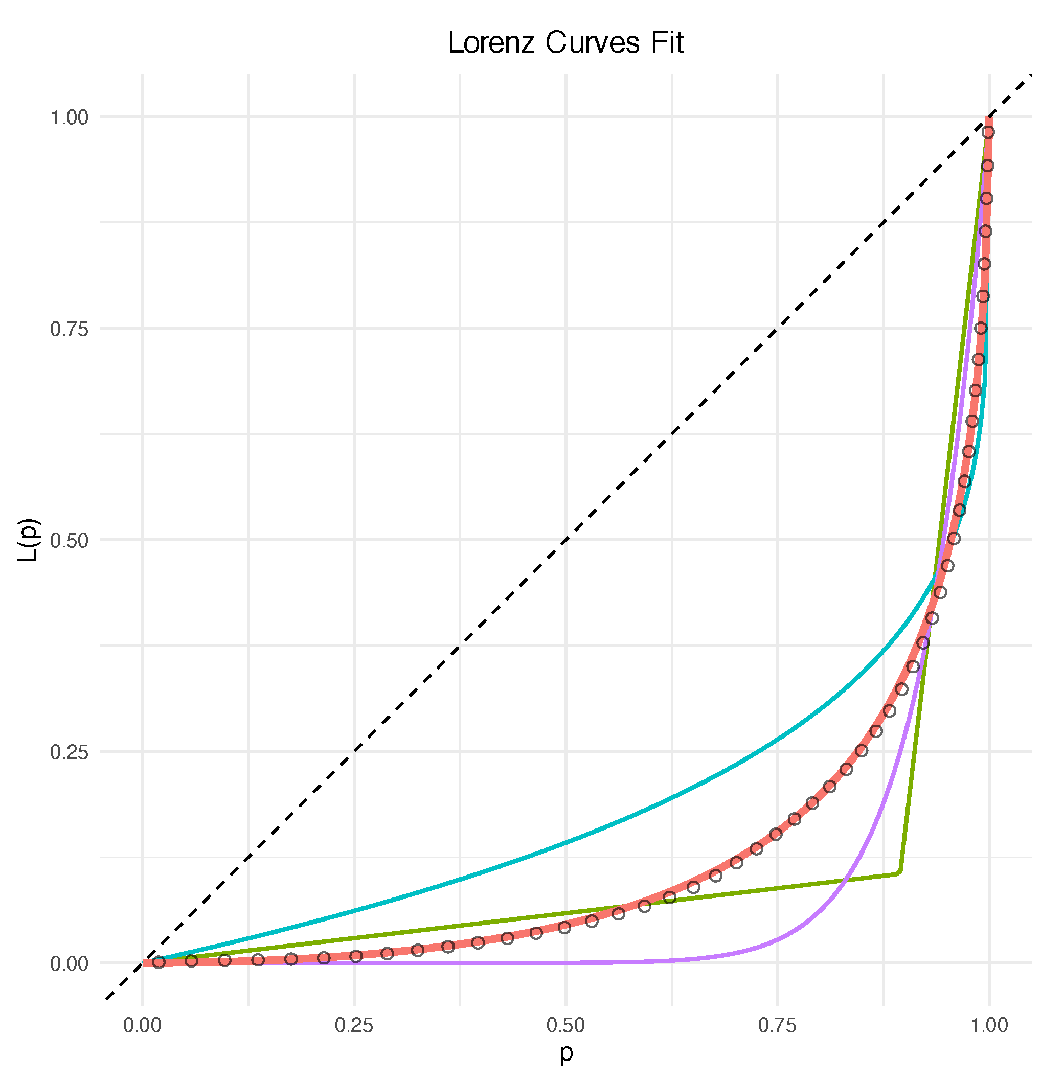
We then transform $\widehat{P}\left(u\right)$ into its corresponding nonparametric Lorenz curve, $\widehat{L}\left(p\right)$, by re-mapping the points according to the geometric argument of Section 3. This empirical Lorenz curve serves as the target for fitting several parametric Lorenz models from Section 4, including the Type I Pareto, the power law, and the Marshall–Olkin and the lognormal families.

Model selection is performed using the Akaike Information Criterion (AIC) and confirmed by visual inspection. As shown in Figure 13, the lognormal Lorenz model provides a decisively superior fit, with an estimated parameter of $\widehat{\sigma }=1.6902$. The other tested families, while representing best fits within their class, provide an unsatisfactory description of the empirical Lorenz curve for the DAX-SMI pair.

Once the parametric Lorenz curve is determined, we numerically invert the $K\left(p\right)$ function using a root-finder (such as uniroot in R) to obtain the corresponding parametric Pickands function via Equation (8). Figure 14 shows this fitted Pickands function against the nonparametric estimate we started from. The close agreement between the two curves confirms the adequacy of the chosen model.

From the lognormal Lorenz model with parameter $\widehat{\sigma }=1.6902$, we compute the dependence indices discussed in Section 6. The results, summarized in

Table 1. Key dependence indices derived from the best-fitting lognormal Lorenz model.

Index	Value	Interpretation
Gini Coefficient (G)	0.768	High overall dependence concentration
Pietra Index (H)	0.602	Strong peak intensity of dependence
Tail Dependence (${\lambda }_U$)	0.602	High probability of joint extreme events
Asymmetry Index (S)	0.000	Perfectly symmetric dependence structure

, reveal a dependence structure that is both symmetric (in line with the symmetry of the lognormal Lorenz model, and the fact that we are considering two well-integrated markets) and strong.

A Gini coefficient of $0.768$ is high, indicating a dependence structure that is far from independence and exhibits significant concentration. This is unsurprising, given the strong economic interdependence between the German and Swiss markets. Because the best-fit model is symmetric ($S=0$), the Pietra index H and the upper tail dependence coefficient ${\lambda }_U$ coincide. Their value of $0.602$ indicates that if one market experiences an extreme positive event, there is an estimated 60.2% probability that the other market does as well, confirming relevant tail co-movement.

Remark 3. 

A crucial consideration for the practical application of our framework, which also represents a key avenue for future research, is its sensitivity to the initial, nonparametric estimation of the Pickands function. The entire chain of analysis—from the empirical Pickands points to the transformed Lorenz curve and the final fitted model—inherits the uncertainty from this first step. Estimators for tail dependence are notoriously data-hungry and can exhibit high variance, an issue compounded by the natural scarcity of data in the joint tails [1,9]. This sensitivity to the choice of estimator and its tuning parameters remains at present the primary bottleneck for the methodology, in those applications where data can be substantially limited. Future work could therefore focus on developing more robust statistical procedures to mitigate these issues. For instance, as we also state in Section 10 below, creating methods to fit Lorenz curve models directly to the data, thereby bypassing the explicit and often unstable estimation of the Pickands function, or developing regularization techniques inspired by inequality theory, could greatly enhance the applicability and reliability of the Pickands–Lorenz connection.

10. Conclusions and Future Directions

We have discussed a one-to-one, geometrically transparent link between two seemingly distant objects: the Pickands dependence function $P\left(u\right)$ that encodes bivariate extreme-value copulas and the Lorenz curve $L\left(p\right)$ that deals with economic inequality.

By rotating, rescaling, and “remapping” the traditional Pickands triangle, we have shown that every admissible $P\left(u\right)$ corresponds to a unique Lorenz curve and vice versa. The mapping is constructive, so that decades of work on tractable Lorenz families can be translated directly into closed-form or easily numerically tractable Pickands functions.

The Lorenz–Pickands bridge enlarges the catalog of practical models, supplies new diagnostic instruments, and offers a fresh angle on the measure-generating function M for the Pickands dependence function and bivariate extreme-value copulas in general. Classical concentration indices like the Gini and the Pietra emerge as scale-free measures of tail dependence, complementing the existing tools.

Using the GDAXI and SMI indices, from Germany and Switzerland, respectively, we have provided a simple example of the application of our methodology. We found that the lognormal Lorenz generates a useful extremal copula to model the dependence between these two indices.

Several promising avenues remain open. Naturally, in terms of empirical analyses, more thorough investigations are needed to compare the performances of the Lorenz representation with existing alternatives, but also to develop those useful heuristics one can conceive by only addressing practical issues.

Further, the present work still relies on $P\left(u\right)$ to obtain an extreme-value copula. An ongoing project is to bypass $P\left(u\right)$ altogether and formulate existence, admissibility, and representation theorems directly in the Lorenz domain. The goal is a “Lorenz calculus” for extremes in which dependence models are manipulated, composed, and constrained using $L\left(p\right)$ only. Because $L\left(p\right)$ is tied to majorization and entropy [48], this could better connect extreme-value dependence to information geometry.

The extension of the Lorenz approach to higher dimensions could also represent an interesting research path, though we envision two possible major issues. From one side, there is no unique generalization of a Lorenz curve in a multivariate framework. One could rely on Lorenz zonoids [30], for instance, but a few alternatives are available in the literature [37], and none appear a priori preferable. From the other side, the Pickands function itself becomes more difficult to treat in higher dimensions [6], and this makes our whole construction more complicated. This is why a fully alternative Lorenz representation of extremal copulas seems to be a better (even if hard to find) option.

From a statistical perspective, standard estimators first recover $P\left(u\right)$ nonparametrically and only then translate results [3,4,7]. Tailored procedures like kernel-type smoothers for $L\left(p\right)$, minimum-distance fitting against Gini-style functionals, or Bayesian priors on Lorenz families could yield lower variance and naturally incorporate inequality-based regularization. Further, many applications call for time-varying or covariate-dependent copulas. The use of $L\left(p\right)$ could help in this direction, thanks to the results in the evolution and transformation of Lorenz curves [14].

All in all, bridging tail dependence and inequality theory does more than simply adding a new trick to the modeler’s toolbox; it possibly sets the stage for a unified language between risk, concentration, and extremes, with many possible applications in finance, economics, and several other fields.