Abstract
In this article, an R-vine copula model is proposed to detect the nonlinear interrelationships between the oil market and five Chinese new-energy-related stock markets from 2017 to 2022, i.e., photovoltaic, new energy vehicles, energy storage, wind power, and nuclear power industries. Firstly, the transmission of downward and upward risk spillover effects (RSEs) is measured from the oil market to the five Chinese new-energy-related stock markets. Subsequently, a CoVaR backtesting methodology is developed to demonstrate the availability of the R-vine copula-CoVaR model. The empirical studies strongly show that the oil market exhibits a significant asymmetric RSE on the five Chinese new-energy-related stock markets. Furthermore, different Chinese new-energy-related stock markets have varying responses to the positive and negative impacts of the oil market. Specifically, the photovoltaic, energy storage, and wind power industries are more sensitive to such adverse effects. However, the new energy vehicle and nuclear power industries are more likely to be positively affected.
MSC:
62P05; 62P20; 91B05; 91G70
1. Introduction
Today oil is still the principal source of energy worldwide. Among the total global energy consumption, oil accounts for 30.95%, remaining the primary energy source globally. The higher the demand for a certain commodity in the national economy, the more closely the market for this commodity is related to the markets of other commodities [1]. Oil is more strongly linked to other markets than ordinary commodities. Due to their scarcity, necessity, and the corresponding futures regime, bulk commodities are at the center of a network of market linkages [2]. Therefore, oil supply and demand changes are closely linked to global economic developments.
Due to the fluctuations in international oil prices, more and more countries have begun to attach importance to the issue of a stable energy supply. Due to the soaring oil prices and the risks associated with oil imports, they have a more urgent need for alternative solutions for energy transition. The emergence of new energy sources has enriched the range of options for energy consumption, reducing pressure on energy demand while balancing green and low-carbon development. Developing new energy sources is also conducive to countries meeting their previously proposed carbon-neutral targets. According to the International Energy Agency [3,4], global demand for renewable energy grew by about 36% from 2015 to 2021. The renewable energy sector is expected to account for two-thirds of global energy investment by 2040.
Behind the long-term rapid economic growth, the import share of China’s oil has continued to rise, from 30.7% in 2001 to 72% in 2021, well above the international safety alert of 50%. New energy has become an important component of China’s multi-wheel drive energy supply system. In March 2021, China proposed to deepen the electricity system reform by building a new electricity system dominated by new energy. Among them, wind power, photovoltaic, and other new energy sources are leading in the power supply structure. According to the published data by the China Electricity Council, the weight of new energy generation in total power generation was on a year-on-year rise from 2017 to 2021. Over the past ten years, the Chinese-installed capacity generation for wind and photovoltaic power has increased by approximately 12 times, reaching 348 million kilowatts and 359 million kilowatts, respectively. It accounted for over 1/3 of the total installed capacity generation for wind and photovoltaic power worldwide and ranked at the top of the world for years. In 2021, sales in China accounted for around 60% of the global sales of new energy vehicles.
In summary, the development of China’s new energy is comprehensive. Its overall scale is at the forefront of the world. A correlation analysis for the oil prices and the stock price of Chinese new energy industries is of great importance for the formulation of energy reform policies in countries around the world, the operation of new energy companies and energy-intensive companies, and investment in this new sector. Our study contributes to the literature in the following directions.
Firstly, new energy includes a variety of non-conventional energy sources. Due to various factors such as geographical location and climate change, countries have different priorities for developing new energy. Existing studies mainly focused on the correlation between traditional energy and the whole new energy industry, and the interactions within the different new-energy-related industries have been neglected. Meanwhile, only a few studied the flourishing Chinese new energy industries. We incorporate new-energy-related industries into the R-vine copula-CoVaR model to portray the RSE of the oil market, enriching the study of risk transmission between the traditional and new energy markets. Our findings will provide additional relevant information for policymakers and investors.
Secondly, we extend the definition of [5] to a multidimensional scenario by combining vine copula and obtain and , which is dimensionless. These new formulations are used to measure the relative magnitude of risk spillovers and to facilitate comparisons of the strength of risk spillovers across multiple markets. Finally, we further develop the CoVaR backtesting methodology [6] for the multidimensional markets and use the proposed method to prove the availability of the R-vine copula-CoVaR model.
This study finds, first, that a significant RSE exits from the oil market to the stock markets in Chinese new-energy-related industries. There are differences in the intensity of risk spillovers in different industries. Power generation industries, such as nuclear power, and downstream industries, such as new energy vehicles, are more sensitive to large fluctuations in oil prices. Second, there are asymmetries in the upward and downward RSE. There are asymmetries in the upside and downside risks spillover effects. In addition, various new energy industries have different sensitivities to positive and negative shocks caused by oil price fluctuations. Chines new-energy-related industries are more sensitive to adverse oil market shocks. By contrast, the new energy vehicle and nuclear power industries are more sensitive to positive surges. Third, we verify the feasibility of calculating the CoVaR based on the R-vine copula model through an extended backtesting method.
Existing research typically focuses on the industry gap between traditional energy sources such as crude oil, coal, and natural gas and new energy sources. However, there is little research on the correlation between different sub-industries in the new energy industry. This article uses the R-vine copula model to study the interdependence between the international crude oil futures market and the Chinese new-energy-related industry stock market, and uses CoVaR to describe the risk spillover effects between the markets; thus, our work further enriches related research.
Studying the interdependence and risk transmission mechanism between markets is beneficial for producers and operators of new energy and high energy-consuming enterprises, which can help them to be aware of the underlying extreme risk and try to control those risks in a timely manner. Our research objective is to measure the risk spillover effects of the international crude oil futures market on the stock markets of various related industries in China’s new energy sector. The main contributions of this article are twofold: (i) We incorporate new-energy-related industries into the R-vine copula CoVaR model to depict the risk spillover effects of the oil market. (ii) We extend the delta-CoVaR to multidimensional situations.
The remainder of this paper is structured as follows. An overview of the relevant studies is provided in Section 2. The research methods are presented in Section 3. In Section 4 we analyze the sample data and obtain the empirical results. In Section 5, we summarize the results and gives some policy recommendations.
2. Literature Review
2.1. The Impact of Oil Price on Stock Price
Because large fluctuations in oil prices are always accompanied by changes in the global situation and the shape of the economy, numerous scholars have studied the relationship between oil prices and the stock market. Kaneko and Lee (1995) [7] concluded that there was some correlation between oil prices and stock prices. Jones and Kaul (1996) [8] compared the volatility spillover relationship between WTI oil prices and stocks in the USA, the UK, Japan, and Canada. They found that volatility spillover relationships were prevalent, but their magnitude varied. The analysis of the oil prices’ impact on stock markets in thirteen European countries and the US can be see in [9]. The study found a significant negative correlation between oil prices and stock returns. Li et al. (2012) [10] examined the oil prices’ impact on the Chinese stock market. They found that an increased oil price had specific positive effects in the long run, which would drive the Chinese stock market in a positive direction.
The quantile-to-quantile approach (Sim and Zhou, 2015) [11] captured the correlation between the distribution of oil price shocks and US stock returns. The conclusion suggested that the relationship between oil prices and the US stock market was asymmetrical. Chen and Lv (2015) [12] found a positive correlation between the oil and Chinese stock markets. Since the onset of the financial crisis in 2008, the correlation coefficient between the two markets has increased to some extent. Bastianin et al. (2016) [13] explored the relationship between oil and stock markets in terms of demand and supply, using a sample of data from G7 member countries. The study results showed that oil on the demand side could have a knock-on effect on the stock markets. Oil, on the supply side, however, did not have a volatile effect on them. Bagchi (2017) [14] focused on the impact of oil price volatility on the stock markets of China, Russia, India, and Brazil BRICs. He found that the volatility of oil prices had an asymmetric effect on the stock markets of these four countries.
Studies about the contagion of Chinese stock market oil prices by examining the difference between extreme positive and negative returns can be seen in [15]; they found that the contagion between oil prices and the stock sector was not negligible and weak. Liu et al. (2017) [16] explored the average and volatility spillovers between the oil market and the stock market using a VAR-GARCH model, concluding that the oil market had a one-way average spillover effect on the Chinese stock market. In addition, the relationship showed a gradual strengthening trend. For more research results about quantile regression model combining GARCH and Copula, please refer to Tian et al. (2022) [17] and references therein; details are omitted here.
2.2. The Impact of Oil Price on the New Energy Stock Market
As a significant power fuel and chemical raw material, oil plays a vital role in economic development. Nevertheless, most major countries have vigorously developed new energy industries to eliminate the two significant problems of resource constraint and environmental pollution. Many scholars discussed the correlation between oil and new energy. Henriques and Sadorsky (2008) [18] reached the conclusion through a VAR model with four variables: the stock prices of renewable energy companies were affected by nine technological stock price shocks, but their responses to oil price shocks were not sensitive. Kumar et al. (2012) [19] integrated the carbon market into their study and found that oil prices, share prices of technology companies, and interest rates played significant roles in the stock prices of clean companies.
In addition, due to the substitution relationship, there was a positive relationship between oil and clean energy returns. Managi and Okimoto (2013) [20], combined with changes in market structure, detected a structural mutation point between November and December 2007 by analyzing smoothed probabilities. Reboredo (2015) [21] investigated systemic risk and dependence between renewable energy and oil markets. Ahmad (2017) [22] proposed an approach to examine the dependence between the three variables of oil prices, the clean energy stock index, and the technology stock index. The findings suggested a strong spillover effect between clean energy and technology stocks but limited dependence on oil prices. Oil may be a better hedge for clean energy stocks than technology stocks.
Reboredo and Ugolini (2018) [23] discussed the sensitivity of renewable energy stock indices in the US and EU to price movements of different types of energy (oil, natural gas, electricity, coal). The quantile regression results showed that changes in energy prices played essential roles in renewable energy price volatility. Oil and electricity prices were the main influences on the volatility of the US and EU new energy stock indices, respectively. Uddin et al. (2019) [24] found that renewable energy (RE) stock returns were positively correlated with changes in oil prices and the total stock index. This correlation was asymmetric, which was higher at longer lags between quartiles.
2.3. Studies Related to Empirical Methodology
The issue of effectively monitoring and preventing financial risk is a common concern to academics and stakeholders. In the 1960s, J.P. Morgan proposed the definition of value-at-risk (VaR) to measure systemic risk, representing the maximum possible loss of a financial asset in the next holding period. VaR can be utilized to prevent risk events in financial markets. However, the method can only analyze individual financial markets and has no way of portraying the spillover of financial risk between markets. The conditional value-at-risk (CoVaR) [25] can be used to describe the extreme value-at-risk that another financial market faces when a certain financial market is in an extreme risk situation.
Quantile regression-based CoVaR provides a valuable tool for measuring the magnitude and direction of linear risk spillovers between financial markets. Subsequently, it has been mainly used to measure the systemic risk of the market (Drakos and Kouretas, 2015; Petrella et al., 2019) [26,27]. Considering the complex and primarily nonlinear correlation between random variables in finance, Girardi and Ergun (2013) [6] proposed a method to measure CoVaR based on a bivariate GARCH model with Engle’s (2002) [28] DCC specification (DCC-GARCH). Trabelsi (2017) [29] utilized this approach to find a substantial risk spillover from oil-producing countries’ oil markets to their stock markets. In recent years, the CoVaR incorporating the Copula function, proposed by Mainik and Schaanning (2014) [30], has been widely used since the gradual emphasis on the study of tail RSE among financial markets. Mensi et al. (2017) [31] studied the extent to which oil prices were dependent on various stock markets during different investment periods, as well as the spillover risk effects in bear markets, bull markets, and normal market conditions.
To address the shortcomings of the aforementioned methods that fail to measure the RSE among multidimensional markets effectively, Reboredo and Ugolini (2015) [32] further integrated the vine copula model to portray the nonlinear tail dependence relationships among multidimensional financial markets. The implied CoVaR discovered the impact of European sovereign debt on the financial system. More studies related to empirical methodology are omitted here.
3. Methodology
3.1. R-vine Copula Model
The Sklar theorem (Sklar, 1959) [33] connects the joint distribution function to the copula as follows:
where is an n-dimensional joint distribution function, and are the marginal distribution functions. To represent complex dependencies among multi-variables, Bedford and Cooke (2001, 2002) [34,35] proposed the regular vine structure based on graph theory.
An R-tree contains a set of tree structures, where each edge of each tree corresponds to a corresponding pair-copula function [36,37]. An R-vine that embodies the dependence relationship between dimensional variables contains tree structures, denoted as . The node set of the tree is , and the edge set is , where . The node set of is the edge set of . If two edges in tree are connected by an edge in tree , then these two edges have the same nodes in tree . The node set in the first tree is , and the edge set is . The joint probability density function of the n-dimensional random variables has the form
where denotes the edge set. is an edge in the . represents the pair-copula function. and are the two conditional nodes connected to e. denotes the set of conditions.
An R-vine structure is constructed to calculate the joint probability density function. The maximum spanning tree algorithm is used to select the optimal R-vine structure with the maximization of [38,39]. The AIC criterion is employed to select pair-copula functions. Some types of copula specifications [40], such as tail independence (Gaussian copula), symmetric tail dependence (Student-t copula, Frank copula), and asymmetric tail dependence (Gumbel copula, Clayton copula), can be used to capture various dependency characteristics, which can be seen in Table 1.

Table 1.
Bivariate copula functions.
3.2. Vine Copula-CoVaR Model
VaR measures the maximum loss that the financial market may experience for a given confidence level. However, the value-at-risk cannot portray the propagation and spillover of financial risk between markets. Adrian and Brunnermei (2011) [25] defined the conditional value-at-risk (CoVaR) as follows:
Obviously, CoVaR formally characterizes the RSE on the market i at moment t when the market j is at the -quantile at-risk-value, i.e., the risk spillover generated at the time . To obtain from Equation (1), we can utilize a copula to simplify the above formula as
where and are the marginal distribution functions of and , respectively. However, the condition set for in Equation (2) does not take into account the impact of more extreme events.
Benoit et al. (2013) [41] modified in Equation (2) and replaced the condition set. The modified CoVaR is denoted as . Consequently, the modified Equation (2) can be expressed as
where is a copula function between and . Setting and , respectively, and taking and as known, we obtain from Equation (3) and then obtain as .
Based on the , Reboredo and Ugolini (2015) [32] employed vine copula to investigate the application of CoVaR in a multidimensional case. In this multivariate conditional setup, is given by
where can refer not only to a single market. Specifically, if market i is conditionally related to market j through the connection of multiple markets, will represent multiple markets. For example, under the assumption that Market 2 is conditionally related to Market 1 through the connection of markets, can be obtained from the vine copula using a four-step procedure:
Step 1: Set the value of -quantile as the value of each unconditional node of the first tree in the vine structure (e.g., ). According to the vine structure and pair-copula function, calculate the value of each node based on the function
where a and b both denote the adjacent conditional node in trees.
Step 2: Taking as calculated in step 1, we can obtain by inverting
Step 3: Repeating the above process, we achieve , ,⋯, in turn.
Step 4: From we can obtain as: .
To explore the effect of different ranges of condition sets on CoVaR, we also need to calculate . The differences in calculating are that Equation (5) used in step 1 is replaced by the following Equation (6):
and in step 2 we obtain by inverting respectively. To visualize the intensity of risk spillovers, Adrian and Brunnermei (2016) [42] introduced the concept of , which can be defined as Based on Abuzayed et al. (2021) [5] introduced as follows:
We continue to extend in Equation (7), based on R-vine copula, to multi-dimensions. Specifically, can be defined as follows:
When we calculate in Equation (8), the value of -quantile in step 1 above is set to 0.5. To compare the intensity of risk spillovers across markets and measure the relative magnitude of risk spillovers, a relative number shall be defined as
3.3. Marginal Distribution Models
The GARCH model [43] extended the ARCH model by reducing the complexity of the parameters and making the lag parameters more flexible, which is proposed as follows:
where represents the conditional mean for under the known information ; is the conditional variance. and . To allow for the skewness and kurtosis, we model the innovation with the skewed t-distribution [44], which has the following density:
where ,
To allow for asymmetric effects between positive and negative asset returns, Zakoian (1994) [45] proposed the TGARCH model that combines threshold autoregression with the GARCH model and takes into account the different effects of negative and positive shocks on volatility. The TGARCH model is of the form
where r denotes the number of thresholds; is a dummy variable, if and otherwise 0; represents the coefficient of asymmetric effect. A larger indicates more significant leverage in the series of returns.
3.4. Backtesting the
Since CoVaR has been expanded into a multidimensional model, we need to develop the CoVaR backtesting methodology (Girardi and Ergun, 2013) [6]. The corresponding test is divided into two steps: First, the eligible data is selected from all samples as the test set according to the conditional information set of CoVaR. The sample size in the test set is T. Second, we count the number of data points in the test set that are smaller than the CoVaR value, denoted as ; N follows a binomial distribution, i.e., . We backtested the with hypothesis vs. . The test statistic is constructed as
Given the significance level , should be rejected if is larger than the critical value. Accordingly, we will prefer to use the adapted model if we cannot deny the null hypothesis.
4. Empirical Results
4.1. Data
The Brent oil market launched by the Intercontinental Exchange (ICE) of the United Kingdom is notable for its breadth and stability. In this empirical study, we considered the daily futures price of Brent crude oil (Brent) to represent the oil market. The CSI New Energy Index was selected to represent the Chinese new energy market, reflecting the overall performance of listed companies in the new energy industry. The companies corresponding to the CSI New Energy Index constituents are divided into segmented industries according to the Shenwan Industry Classification. Five of the most high-frequency industries, i.e., photovoltaic, energy storage, new energy vehicles, wind power, and nuclear power industries, were selected as typical new energy industries for subsequent research and analysis from 1 January 2017 to 26 July 2022. The closing prices of the CSI PV Index (PV), the CSI New Energy Vehicle Index (VEHICLES), the CSI Energy Storage Index (STORAGE), the CSI Wind Power Index (WIND), and the CSI Nuclear Power Index (NUCLEAR) are denoted to represent the above five industry stock markets. All the above data were obtained from Wind Information Co., Ltd. (Shanghai, China). The data of Chinese new-energy-related stock markets were converted to US dollar prices based on spot rates. After excluding non-trading days, 1341 sets of valid data were retained. The long-term trends of the different CSI Index price indices and the Brent oil price can be seen in Figure 1. Figure 2 plots the returns, which are given as , and denotes the closing price of the financial market.
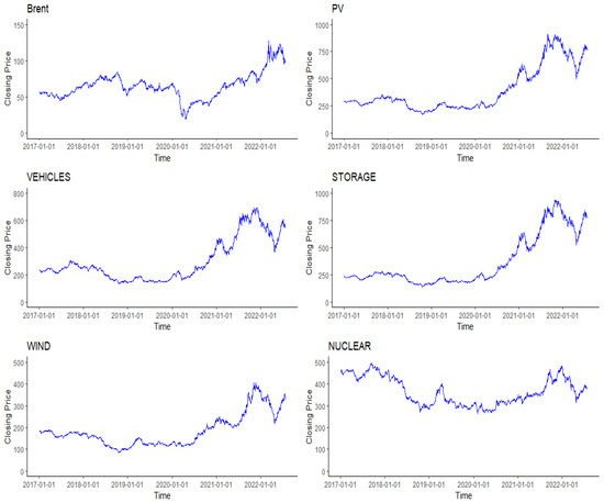
Figure 1.
The Brent oil price and different CSI Index price indices.
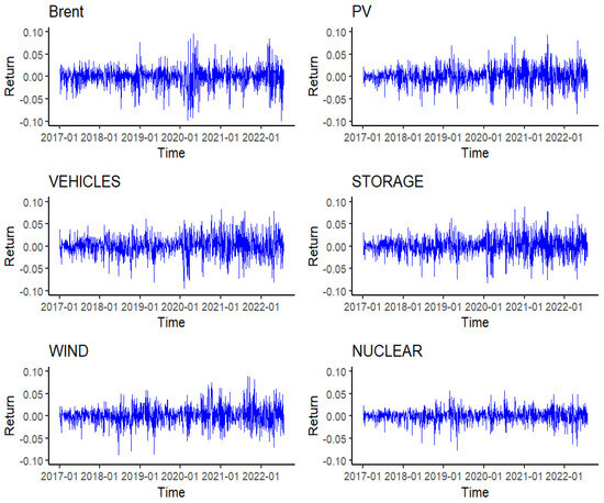
Figure 2.
Returns of the different financial markets.
Table 2 reports the descriptive statistical results of these financial market returns, from which it can be seen that, firstly, due to the arbitrage equilibrium, the means of financial market returns are approximately zero. According to the standard deviation, the stock market price indices of PV and energy storage rise sharply, with more effective means and minor standard deviations. Oil prices fluctuate significantly. Only the Chinese nuclear energy market returns have a negative mean, demonstrating that it has had more days of decline and a more significant decline than an increase. Secondly, all financial markets have negative skewness coefficients, with a significant left-hand bias, implying a greater likelihood of significant price declines in each financial market. The kurtosis coefficients for all financial markets are more prominent than 3, consistent with the properties of sharp peaks. Thirdly, stock returns are not normal according to Jarque–Bera statistics. Because of the left-skewed characteristics of the spikes, the skewed t-distribution is preferred to fit the marginal distribution of the series in the subsequent model fitting. Finally, Engle’s Lagrange Multiplier (LM) test indicates that, at a 5% significance level, there is an autoregressive conditional heteroskedasticity effect in the financial return sequence.
Table 2.
Descriptive statistics of returns of stock markets and the oil market.
4.2. The Marginal Distributions
We chose the values of parameters in the ARMA model based on the principle of maximizing the BIC values, and the optimal value for both parameters is 0. For the marginal distribution of returns in the oil and stock markets, we initially employed the TGARCH model with a skewed t-distribution to construct it, in order to eliminate heteroscedasticity and the asymmetry of positive and negative disturbances. The estimation results show that only the asymmetric effect term coefficient of Brent oil returns is significantly valid. Since there is no short-selling mechanism in the Chinese stock market, the five stock markets’ leverage effect is insignificant. Therefore, the marginal distribution of the return series of the Brent oil market is built on the TGARCH model with the skewed t-distribution. The marginal distributions of the returns of the five Chinese new-energy-related industry stock markets are built on the GARCH model with the skewed t-distribution.
Table 3 presents the estimated values of the model parameters, the Ljung–Box test, and ARCH tests, which are used to evaluate the adequacy of the model. The coefficient of the asymmetric effect for the oil returns is significantly greater than zero, which indicates that bearish news has more significant impacts on the oil market than good news. The Ljung–Box test was applied to the standardized residuals of the TGARCH(1,1) model with a skewed t-distribution. The results did not reject the of the autocorrelation of lag 20 at the 5% significance level. Engle’s LM test indicates that, at the 5% significance level, there is no ARCH effect in any of the yield series. The estimated values of the parameters and their standard deviations indicate that the TGARCH(1,1) model is appropriate. We also verified the applicability of the skewed t-distribution model by testing the null hypothesis (i.e., the standardized residuals are uniformly distributed (0, 1)). Therefore, we adopted the well-known Kolmogorov–Smirnov test method, which compares the sample distribution of standardized residuals with the theoretical distribution. The p-values listed in the last rows of Table 3 indicate that, at the 5% significance level, the null hypothesis that the distribution function is correctly set cannot be rejected. Therefore, the evidence provided by the adjusted Pearson goodness-of-fit test indicates that there are no errors in the specification of these marginal distribution models.
Table 3.
Parameter estimates of TGARCH(1,1) model and GARCH(1,1) model with the skewed t-distribution.
4.3. Estimation and Selection of the Copulas
We estimate three vine copula models, R-vine, C-vine, and D-vine, respectively, in this section. The optimal R-vine and C-vine structures were selected using the maximum spanning tree algorithm. The node order of D-vine was chosen with the repetitive nearest neighbor algorithm [46] to improve the fitting effect. The optimal pair-copula function for each edge was selected according to the AIC. Table 4 shows the evaluation of the three vine structures. The R-vine structure performs the best, followed by C-vine and D-vine. Furthermore, the Vuong test [47] was applied to the three vine structures in pairs, and the results are shown in Table 5. The p-values for these tests indicate that R-vine and C-vine are more suitable than D-vine. Napoles (2010) [48] pointed out that R-vine has a diverse and more flexible dependency structure. We utilized the R-vine structure to construct the subsequent model due to the smaller AIC and BIC values.
Table 4.
The evaluation of the three vine structures.
Table 5.
Vuong test for three vine structures.
Figure 3 illustrates the tree’s structure at each level of the constructed R-vine copula model. We conducted the goodness-of-fit test by combining the PIT with the ECP [49] to verify the validity of the model. The p-value is 0.855. This indicates that at the 5% significance level, the null hypothesis that the distribution function is correctly set cannot be rejected, thereby demonstrating that the model is valid. Nodes 1, 2, 3, 4, 5, and 6 correspond to the Brent oil market, the stock market of the Chinese photovoltaic industry, the Chinese new energy vehicle industry, the Chinese energy storage industry, the Chinese wind power industry, and the Chinese nuclear power industry, respectively.
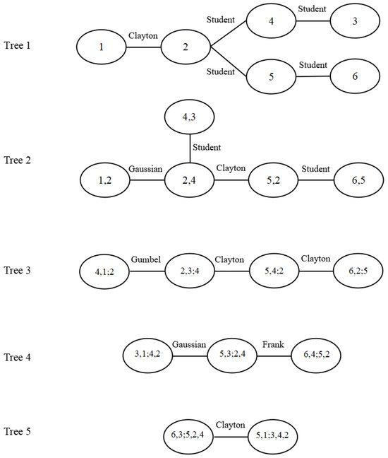
Figure 3.
Interdependent structure of financial markets.
Table 6 shows the parameter estimates of each pair copula in the R-vine copula. The optimal copula functions between stock markets in the Chinese new-energy-related industry are all Student-t copula functions. The dependence of the upper and lower tails between each financial market can be better captured. The upper- and lower-tail dependence between stock markets in the Chinese new-energy-related industry is symmetric and has a strong positive correlation. The Brent oil market is correlated with the Chinese PV stock market and the energy storage stock market in China through the Clayton copula. It indicates that the Brent oil market has an asymmetric dependence on both stock markets, with a stronger lower-tail dependence than upper-tail dependence. In addition, there is a weak positive correlation between the markets, suggesting a greater probability of simultaneous declines in the market indices.
Table 6.
Parameter estimates of R-vine copula model.
The copula functions between the Brent oil market and with stock markets of the Chinese energy storage and wind power industries are Gaussian copula, indicating no tail dependence of these two markets. There is also a weak negative correlation because the correlation coefficients are negative. The Brent oil market is connected to the stock market of the Chinese new energy vehicle industry through the Gumbel copula, indicating an asymmetric dependence on the stock market with a stronger up-tail dependence. There is a weak positive correlation, suggesting that the indices are more likely a simultaneous rise.
4.4. Risk Spillovers from Oil to Five NE Stock Markets
Based on the R-vine copula model, according to the method described in Section 3.2, we calculated , , and to measure the RSE of the Brent oil market on the Chinese new energy industry stock markets. Figure 4 illustrates the variations of VaR and CoVaR for the five stock markets at a 95% confidence level.
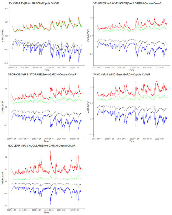
Figure 4.
VaR and CoVaR. Notes: In each subfigure, the black and green lines stand for the VaRs of each stock market. The blue lines stand for the downward risk spillovers. This red line represents the upward RSE of the Brent crude oil market on the Chinese NE stock markets.
In view of Figure 4, it is clear that information spillover from the surge and crash in the Brent oil market has exacerbated the risk exposure of the Chinese new-energy-related stock markets. The steady downward revision of oil production from 2017 to 2018 was influenced by political factors such as US sanctions against Iran and natural factors such as increased pressure on US Gulf Coast refining due to frequent hurricanes. At the same time, oil prices had steadily risen as the global economy returned to recovery, increasing the RSE on Chinese new-energy-related stock markets, particularly in midstream and downstream manufacturing industries such as new energy vehicles. Around 2018, US energy companies broke records in oil production from oil rigs and shale basins. Surging supply and concerns about shrinking demand continued to weigh on oil prices. Meanwhile, the downward risk value of the Chinese new-energy-related stock markets has gradually increased along with the rising trade friction between the US and China.
In early 2020, Saudi Arabia started an oil price war by cutting prices and increasing production. Oil prices in the international market plummeted for a time due to the COVID-19, the world recession, and the imbalance between oil supply and demand, and the spillover effect of oil on new energy stock markets increased. After April 2020, oil demand picked up as more and more countries resumed work and production while preventing and controlling the outbreak. In addition, the supply side of the oil market is tightening. Oil prices rise slowly, with the spillover effect diminishing.
Global gas and coal prices rose sharply in 2021, forcing many power generators to switch from gas to oil and diesel. Oil-producing countries could not meet market demand even after increasing production, fueling a spike in oil prices in October of that year. The spillover effect had increased significantly, with the impacts on the wind, nuclear, and photovoltaic power generation industries becoming more pronounced. In the first half of 2022, oil prices continued to rise and break new highs, supported by factors such as supply risk concerns arising from the Russia–Ukraine situation, with increased RSE.
Table 7 shows the mean values of CoVaR and the results of the tests for RSE. It can be observed that the Brent oil market has a significant RSE on the Chinese new energy stock markets, and the positive and negative spillover effects of this risk are asymmetric. The extreme upward risk in the Brent oil market is shown as a positive sign by investors in the new energy industry that demand for energy in the manufacturing sector is rising between now and sometime in the future and that the market will be in a state that supplies less than demand. This expectation is conducive to driving increased upward risk in the new energy industry. China is re-planning to develop the nuclear power sector, vulnerable to more volatile market influences from other new energy industries. The rapid rise in oil prices has forced more consumers to opt for new energy vehicles, and as a result, stocks in the new energy vehicle industry have risen sharply. The average value of for both industries is more significant than 100%.
Table 7.
Results of RSE and significance test.
In the last two decades, oil prices have been strongly reflected in many international events, such as geopolitical conflicts and financial crises. Fluctuations in energy prices have further influenced regional and even international situations. Investors see the extreme downward risk in the Brent oil market as a warning of instability or recession. Investors are concerned about the reduced demand for energy in the manufacturing sector, and the corresponding stock markets are facing enormous structural selling pressure. Consequently, there is a significant increase in the negative spillover effect from the oil market to the stock markets of new energy, especially new energy generation industries such as nuclear and wind power.
In order to examine the impact of changes in the set of conditions, comparing and in Table 7, it can be found that the absolute value of the mean of each is more significant than , indicating that the occurrence of more extreme events in the oil market has increased the risk to the Chinese new-energy-related stock markets. We use the Kolmogorov–Smirnov test to verify the upward and downward RSE, which compares the CoVaR and VaR. These p-values indicate that the null hypothesis can be rejected at a 1% significance level, thereby proving the existence of a two-way spillover effect of risks from the oil market to the Chinese new-energy-related stock markets.
Comparing the mean of , we find significant differences, which indicates that the upward and downward RSE may be asymmetrical. Furthermore, we performed Wilcoxon signed-rank tests on the . The results show that for the tests of new energy vehicles and the nuclear energy industry, the p-values indicate that the null hypothesis can be rejected at a 1% significance level, which means that the spillover effect of downward risks is significantly higher than that of upward risks. The Wilcoxon signed-rank test results for the new energy vehicle and nuclear energy industries indicate the opposite situation. This implies that the upward RSE of the oil market on these two stock markets is significantly greater than the downward RSE.
4.5. CoVaR Backtesting Results
The backtesting approach mainly includes two steps. Firstly, based on the condition information set, we selected the data that meets the conditions from all the samples and used it as the test sample with a size of T. Secondly, let N represent the number of events where the loss exceeds CoVaR in the test samples, which is the total number of days with a log return rate lower than CoVaR, then one has . The null hypothesis is vs. the alternative hypothesis . Then the likelihood ratio test statistic is constructed as
The risk assessment of the model performs well if the null hypothesis cannot be rejected.
We backtested the CoVaR for the conditional coverage properties. The data that meets the condition set of , was selected as the test sample. The LR test statistic was calculated according to Equation (10). The test results are shown in Table 8.
Table 8.
Test statistics and p-values for CoVaR conditional coverage properties.
The p-values of Table 8 indicate that, at the 5% significance level, cannot be rejected. Therefore, the R-vine copula-CoVaR model effectively measures risk spillovers between multidimensional markets by considering the transmission of risk information across multiple markets.
5. Conclusions
In order to measure the RSE of the oil on the Chinese new-energy-related stock markets, we select the daily closing prices of the Brent oil market, the CSI PV Index, the CSI New Energy Vehicle Index, the CSI Energy Storage Index, the CSI Wind Power Index, and the CSI Nuclear Power Index for the period from January 1, 2017, to July 26, 2022, as the research subjects. First, an R-vine copula model is proposed to detect the nonlinear interdependence between the oil market and the five Chinese new-energy-related stock markets. Second, following Reboredo and Ugolini (2015) [32], we calculate the , , and to measure the upward and downward RSE. Finally, we develop the CoVaR backtesting methodology [6] for the R-vine copula-CoVaR model.
The empirical studies conclude as follows. Firstly, the oil market has a significant RSE on Chinese new-energy-related stock markets. There are differences in the intensity of risk spillovers in different industries. The power generation industry, such as nuclear power, and the downstream industry, such as new energy vehicles, are more sensitive to large fluctuations in oil prices.
Secondly, there is an asymmetry in the upward and downward RSE. Furthermore, different Chinese new-energy-related stock markets have different performances due to the positive and negative impacts of the oil market. The photovoltaic, energy storage, and wind power industries are more sensitive to adverse impacts in the Brent oil market. The new energy vehicle and nuclear power industries are more sensitive to positive impacts.
Thirdly, through CoVaR backtesting, the R-vine copula-CoVaR model can be considered an adequate measure of risk spillovers between multidimensional markets by considering the transmission of risk information across multiple markets.
Finally, based on these findings, we provide important implications for international capital holders and supervisory authorities optimizing investment portfolios and formulating supervision policy. For policymakers, they should pay attention to the tail risk caused by the sharp fluctuations in international oil prices and formulate relevant policies to deal with the spillover effect of the sharp fluctuations in oil prices on the share prices of the new energy industry and further avoid the impact on the capital market as a whole. Based on the information that RSE and strong correlations among new-energy-related industries, relevant enterprises should actively cooperate to reduce the impact of oil price fluctuations on themselves so that the new energy industry can achieve synergistic development.
Author Contributions
Conceptualization, M.Z.; methodology, K.Z.; formal analysis, X.X.; investigation, K.Z. and X.X.; data curation, X.X.; writing—original draft, M.Z.; funding acquisition, M.Z. All authors have read and agreed to the published version of the manuscript.
Funding
This research was funded by the Social Science Foundation of the Anhui Province of China (No.: AHSKF2022D08).
Data Availability Statement
Data will be made available on request.
Conflicts of Interest
The authors declare no conflicts of interest.
References
- Jensen, G.R.; Johnson, R.R.; Mercer, J.M. Efficient use of commodity futures in diversified portfolios. J. Futures Mark. 2000, 20, 489–506. [Google Scholar] [CrossRef]
- Erb, C.B.; Harvey, C.R. The strategic and tactical value of commodity futures. Financ. Anal. J. 2006, 62, 69–97. [Google Scholar] [CrossRef]
- International Energy Agency (IEA). Tracking Clean Energy Progress; IEA: Paris, France, 2017. [Google Scholar]
- International Energy Agency (IEA). World Energy Outlook; IEA: Paris, France, 2018. [Google Scholar]
- Abuzayed, B.; Bouri, E.; Al-Fayoumi, N.; Jalkh, N. Systemic risk spillover across global and country stock markets during the COVID-19 pandemic. Econ. Anal. Policy 2021, 71, 180–197. [Google Scholar] [CrossRef]
- Girardi, G.; Ergun, A.T. Systemic risk measurement: Multivariate GARCH estimation of CoVaR. J. Bank Financ. 2013, 37, 3169–3180. [Google Scholar] [CrossRef]
- Kaneko, T.; Lee, B.S. Relative importance of economic factors in the U.S. and Japanese stock markets. J. Jpn. Inst. Econ. 1995, 9, 290–307. [Google Scholar] [CrossRef]
- Jones, C.M.; Kaul, G. Oil and the stock markets. J. Financ. 1996, 51, 463–491. [Google Scholar] [CrossRef]
- Park, J.; Ratti, R.A. Oil price shocks and stock markets in the US and 13 European countries. Energy Econ. 2008, 30, 2587–2608. [Google Scholar] [CrossRef]
- Li, S.F.; Zhu, H.M.; Yu, K.M. Oil prices and stock market in China: A sector analysis using panel cointegration with multiple breaks. Energy Econ. 2012, 34, 1951–1958. [Google Scholar] [CrossRef]
- Sim, N.; Zhou, H.T. Oil prices, US stock return, and the dependence between their quantiles. J. Bank Financ. 2015, 55, 1–8. [Google Scholar] [CrossRef]
- Chen, Q.; Lv, X. The extreme-value dependence between the crude oil price and Chinese stock markets. Int. Rev. Econ. Financ. 2015, 39, 121–132. [Google Scholar] [CrossRef]
- Bastianin, A.; Conti, F.; Manera, M. The impacts of oil price shocks on stock market volatility: Evidence from the G7 countries. Energy Policy 2016, 98, 160–169. [Google Scholar] [CrossRef]
- Bagchi, B. Volatility spillovers between crude oil price and stock markets: Evidence from BRIC countries. Int. J. Emerg. Mark. 2017, 12, 352–365. [Google Scholar] [CrossRef]
- Fang, S.; Egan, P. Measuring contagion effects between crude oil and Chinese stock market sectors. Q. Rev. Econ. Financ. 2018, 68, 31–38. [Google Scholar] [CrossRef]
- Liu, Z.H.; Ding, Z.H.; Li, R.; Jiang, X.; Wu, J.; Lv, T. Research on differences of spillover effects between international crude oil price and stock markets in China and America. Nat. Hazards 2017, 88, 575–590. [Google Scholar] [CrossRef]
- Tian, M.X.; Alshater, M.M.; Yoon, S.M. Dynamic risk spillovers from oil to stock markets: Fresh evidence from GARCH copula quantile regression-based CoVaR model. Energy Econ. 2022, 115, 106341. [Google Scholar] [CrossRef]
- Henriques, I.; Sadorsky, P. Oil prices and the stock prices of alternative energy companies. Energy Econ. 2008, 30, 998–1010. [Google Scholar] [CrossRef]
- Kumar, S.; Managi, S.; Matsuda, A. Stock prices of clean energy firms, oil and carbon markets: A vector autoregressive analysis. Energy Econ. 2012, 34, 215–226. [Google Scholar] [CrossRef]
- Managi, S.; Okimoto, T. Does the price of oil interact with clean energy prices in the stock market? Jpn. World Econ. 2013, 27, 1–9. [Google Scholar] [CrossRef]
- Reboredo, J.C. Is there dependence and systemic risk between oil and RE stock prices? Energy Econ. 2015, 48, 32–45. [Google Scholar] [CrossRef]
- Ahmad, W. On the dynamic dependence and investment performance of crude oil and clean energy stocks. Res. Int. Bus. Financ. 2017, 42, 376–389. [Google Scholar] [CrossRef]
- Reboredo, J.C.; Ugolini, A. The impact of energy prices on clean energy stock prices. A multivariate quantile dependence approach. Energy Econ. 2018, 76, 136–152. [Google Scholar] [CrossRef]
- Uddin, G.S.; Rahman, M.L.; Hedstrom, A.; Ahmed, A. Cross-quantilogram-based correlation and dependence between renewable energy stock and other asset classes. Energy Econ. 2019, 80, 743–759. [Google Scholar] [CrossRef]
- Adrian, T.; Brunnermeier, M.K. CoVaR; Working Paper; Federal Reserve Bank of New York: New York, NY, USA, 2011. [Google Scholar]
- Drakos, A.A.; Kouretas, G.P. Bank ownership, financial segments and the measurement of systemic risk: An application of CoVaR. Int. Rev. Econ. Financ. 2015, 40, 127–140. [Google Scholar] [CrossRef]
- Petrella, L.; Laporta, A.G.; Merlo, L. Cross-country assessment of systemic risk in the European stock market: Evidence from a CoVaR Analysis. Soc. Indic. Res. 2019, 146, 169–186. [Google Scholar] [CrossRef]
- Engle, R. Dynamic conditional correlation: A simple class of multivariate generalized autoregressive conditional heteroskedasticity models. J. Bus. Econ. Stat. 2002, 20, 339–350. [Google Scholar] [CrossRef]
- Trabelsi, N. Tail dependence between oil and stocks of major oil-exporting countries using the CoVaR approach. Borsa Istanb. Rev. 2017, 17, 228–237. [Google Scholar] [CrossRef]
- Mainik, G.; Schaanning, E. On dependence consistency of CoVaR and some other systemic risk measures. Stat. Risk Model. 2014, 31, 49–77. [Google Scholar] [CrossRef]
- Mensi, W.; Hammoudeh, S.; Shahzad, S.J.H.; Shahbaz, M. Modeling systemic risk and dependence structure between oil and stock markets using a variational mode decomposition-based copula method. J. Bank Financ. 2017, 75, 258–279. [Google Scholar] [CrossRef]
- Reboredo, J.C.; Ugolini, A. A vine-copula conditional value-at-risk approach to systemic sovereign debt risk for the financial sector. N. Am. Econ. Financ. 2015, 32, 98–123. [Google Scholar] [CrossRef]
- Sklar, A. Fonction de répartition à n Dimensions et leurs Marges. Publ. L’Institut Stat. L’Université Paris 1959, 8, 229–231. [Google Scholar]
- Bedford, T.; Cooke, R.M. Probability density decomposition for conditionally dependent random variables modeled by vines. Ann. Math. Artif. Intell. 2001, 32, 245–268. [Google Scholar] [CrossRef]
- Bedford, T.; Cooke, R.M. Vines—A new graphical model for dependent random variables. Ann. Statist. 2002, 30, 1031–1068. [Google Scholar] [CrossRef]
- Kurowicka, D.; Cooke, R.M. Completion problem with partial correlation vine. Linear Alg. Appl. 2006, 418, 188–200. [Google Scholar] [CrossRef]
- Aas, K.; Czado, C.; Frigessi, A.; Bakken, H. Pair-copula constructions of multiple dependence. Insur. Math. Econ. 2009, 44, 182–198. [Google Scholar] [CrossRef]
- Brechmann, E.C.; Czado, C.; Aas, K. Truncated regular vines in high dimensions with application to financial data. Can. J. Stat.-Rev. Can. Stat. 2012, 40, 68–85. [Google Scholar] [CrossRef]
- Dissmann, J.; Brechmann, E.C.; Czado, C.; Kurowicka, D. Selecting and estimating regular vine copulae and application to financial returns. Comput. Stat. Data Anal. 2013, 59, 52–69. [Google Scholar] [CrossRef]
- Nelsen, R.B. An Introduction to Copulas; Springer: New York, NY, USA, 2006. [Google Scholar]
- Benoit, S.; Colletaz, G.; Hurlin, C.; Prignon, C. A Theoretical and Empirical Comparison of Systemic Risk Measures. HEC Paris Research Paper FIN-2014-1030. 2013. Available online: https://shs.hal.science/halshs-00746272v2 (accessed on 11 May 2025).
- Adrian, T.; Brunnermeier, M.K. CoVaR. Am. Econ. Rev. 2016, 106, 1705–1741. [Google Scholar] [CrossRef]
- Bollerslev, T. Generalized autoregressive conditional heteroscedasticity. J. Econ. 1986, 31, 307–327. [Google Scholar]
- Hansen, B. Autoregressive conditional density estimation. Int. Econ. Rev. 1994, 35, 705–730. [Google Scholar] [CrossRef]
- Zakoian, J.M. Threshold heteroskedastic models. J. Econ. Dyn. Control. 1994, 18, 931–955. [Google Scholar] [CrossRef]
- Rosenkrantz, D.J.; Stearns, R.E.; Lewis, P.M., II. An analysis of several heuristics for the traveling salesman problem. SIAM J. Comput. 1977, 6, 563–581. [Google Scholar] [CrossRef]
- Vuong, Q.H. Likelihood ratio tests for model selection and non-nested hypotheses. Econometrica 1989, 57, 307–333. [Google Scholar] [CrossRef]
- Napoles, O.M. Bayesian Belief Nets and Vines in Aviation Safety and Other Applications. Ph.D. Thesis, Delft Institute of Applied Mathematics, Delft, The Netherlands, 2010. [Google Scholar]
- Genest, C.; Remillard, B.; Beaudoin, D. Goodness-of-fit tests for copulas: A review and a power study. Insur. Math. Econ. 2009, 44, 199–213. [Google Scholar] [CrossRef]
Disclaimer/Publisher’s Note: The statements, opinions and data contained in all publications are solely those of the individual author(s) and contributor(s) and not of MDPI and/or the editor(s). MDPI and/or the editor(s) disclaim responsibility for any injury to people or property resulting from any ideas, methods, instructions or products referred to in the content. |
© 2025 by the authors. Licensee MDPI, Basel, Switzerland. This article is an open access article distributed under the terms and conditions of the Creative Commons Attribution (CC BY) license (https://creativecommons.org/licenses/by/4.0/).