Enhanced Ratio-Type Estimators in Adaptive Cluster Sampling Using Jackknife Method

Abstract

Adaptive cluster sampling is a methodology designed for data collection in contexts where the population is rare and spatially clustered. This approach has been effectively applied in various disciplines, including epidemiology and resource management. The present study introduces novel estimators that incorporate auxiliary variable information to improve estimation efficiency. These estimators were developed using the jackknife resampling technique to improve the performance of ratio-type estimators. Theoretical properties, including bias and mean square error (MSE), were derived, and a simulation study was conducted to validate the theoretical findings. The results demonstrated that the proposed estimators consistently outperformed conventional estimators that do not utilize auxiliary variables across all network sample sizes. Furthermore, in several scenarios, the proposed estimators also exhibited superior efficiency to existing ratio estimators that do incorporate auxiliary information.

1. Introduction

Sampling methods are employed when it is impractical to collect data from an entire population. To ensure the validity of statistical inferences, it is essential that the sample be obtained through probability-based sampling techniques. One of the most widely used probability sampling methods is simple random sampling. The population mean for a variable of interest is typically estimated using the sample mean, which is known to be an unbiased estimator. A central objective in sampling theory is to enhance the efficiency of such estimators.

In many cases, the estimation efficiency can be enhanced by utilizing an auxiliary variable that is correlated with the variable of interest. When both variables exhibit a high positive correlation, the ratio estimator, which incorporates the auxiliary variable’s mean, is widely adopted. Numerous studies have proposed improvements to the ratio estimator in the context of simple random sampling. For example, Sisodia and Dwivedi [1] introduced a modified ratio estimator based on the coefficient of variation of the auxiliary variable. Singh and Tailor [2] proposed an estimator that incorporates the population correlation coefficient between the target and auxiliary variables. Yadav et al. [3] developed ratio-cum-product estimators, while Jerajuddin and Kishun [4] enhanced ratio estimators by considering sample size. Soponviwatkul and Lawson [5] proposed further refinements by incorporating the coefficient of variation, correlation coefficient, and regression coefficient.

However, in situations where the population is both rare and clustered, simple random sampling may not be optimal. To address this, Thompson [6] introduced adaptive cluster sampling (ACS) in 1990. In ACS, an initial sample is selected using simple random sampling without replacement. If a unit in this initial sample satisfies a prespecified condition for the variable of interest, its neighboring units are added to the sample. This expansion continues iteratively until no additional units meet the condition. The collection of initial and subsequently added units forms a network. Units that do not meet the condition are referred to as edge units. The union of a network and its edge units constitutes a cluster. If the initial unit fails to satisfy the condition, it remains a singleton network. For this study, neighborhoods were defined as the four orthogonally adjacent units (up, down, left, and right), with mutual neighborhood relationships assumed (Figure 1). ACS has proven effective across a range of survey applications, especially in situations where the target attribute is either rare or exhibits spatial clustering. Numerous studies have employed ACS in diverse fields, including forest ecosystem monitoring [7], herpetofaunal surveys in tropical rainforests [8], evaluations of sea lamprey larval distributions [9], and investigations of freshwater mussel populations [10]. The method has also been utilized in hydroacoustic sampling [11] and in research related to the COVID-19 pandemic [12,13,14]. Beyond ecological and epidemiological contexts, ACS has also been adapted for autonomous systems and Internet of Things (IoT) applications [15,16].

Thompson also proposed an estimator and demonstrated that ACS yields improved efficiency in clustered populations. Analogously to simple random sampling, incorporating auxiliary variable information in ACS can further improve estimator performance. Chao [17] introduced a ratio estimator for ACS, while Dryver and Chao [18] introduced modified ratio estimators. Chutiman and Kumphon [19] presented a ratio estimator using two auxiliary variables. Chutiman [20] and Yadav et al. [21] proposed ratio estimators based on population parameters, including the coefficient of variation, kurtosis, skewness, and correlations with auxiliary variables. Chaudhry and Hanif [22,23] proposed generalized exponential-type estimators, while Bhat et al. [24] developed a generalized class of ratio-type estimators.

Although several studies have proposed enhancements to ratio-type estimators within the framework of ACS, a comprehensive investigation into the application of jackknife resampling techniques for refining ratio-type estimators under ACS remains limited in the existing literature. This study addresses this gap by developing an enhanced version of Chao’s ratio-type estimator for adaptive cluster sampling, which uses the jackknife method to leverage data from a single auxiliary variable, specifically the auxiliary variable’s mean. Section 2 outlines relevant estimators in ACS, Section 3 introduces the proposed jackknife-based estimators, Section 4 presents simulation results, and Section 5 concludes the study.

2. Adaptive Cluster Sampling

In adaptive cluster sampling, an initial sample of units is selected using simple random sampling without replacement.

Let $y$ and $x$ denote the variable of interest and the auxiliary variable, respectively. Let $n$ represent the initial sample size and $\nu$ be the final sample size. Let ${\psi }_i$ denote the network that includes unit $i$, and let $m_i$ represent the number of units in that network.

Let ${\left(w_y\right)}_i$ and ${\left(w_x\right)}_i$ denote the averages of the y- and x-values, respectively, within the network that includes the initial sample unit $i$, where ${\left(w_y\right)}_i={\displaystyle \frac{1}{m_i}}{\displaystyle \sum _{j\in {\psi }_i}{y}_j}$ for the variable of interest and ${\left(w_x\right)}_i={\displaystyle \frac{1}{m_i}}{\displaystyle \sum _{j\in {\psi }_i}{x}_j}$ for the auxiliary variable.

The Hansen–Hurwitz estimator of the population mean for the variable of interest is [25]:

$${\overline{w}}_y={\displaystyle \frac{1}{n}}{\displaystyle \sum _{i=1}^n{\left(w_y\right)}_i}$$

(1)

The mean square error (MSE) of ${\overline{w}}_y$ is:

$$MSE\left({\overline{w}}_y\right)=\left(1-f_n\right){\displaystyle \frac{S_{wy}^2}{n}},$$

(2)

where $f_n={\displaystyle \frac{n}{N}}$ and $S_{wy}^2={\displaystyle \frac{1}{\left(N-1\right)}}{\displaystyle \sum _{i=1}^n{\left[{\left(w_y\right)}_i-{\mu }_y\right]}^2}$.

The modified Hansen–Hurwitz estimator of the population mean of the auxiliary variable is:

$${\overline{w}}_x={\displaystyle \frac{1}{n}}{\displaystyle \sum _{i=1}^n{\left(w_x\right)}_i}$$

(3)

Let $R$ be the population ratio between $y$ and $x$, $R={\displaystyle \frac{{\mu }_y}{{\mu }_x}}$. Chao [17] introduced the following ratio estimator for the population mean:

$${\overline{w}}_R=\left({\displaystyle \frac{{\overline{w}}_y}{{\overline{w}}_x}}\right){\mu }_x=\hat{R}{\mu }_x$$

(4)

where ${\overline{w}}_R$ is a biased estimator of ${\mu }_y$. The bias of ${\overline{w}}_R$ is:

$$Bias\left({\overline{w}}_R\right)={\displaystyle \frac{{\mu }_y}{n}}\left(1-f_n\right)C_{wx}\left(C_{wx}-{\rho }_{wx\cdot wy}{C}_{wy}\right),$$

(5)

where $C_{wx}={\displaystyle \frac{S_{wx}}{{\mu }_x}}$, $S_{wy}^2={\displaystyle \frac{1}{\left(N-1\right)}}{\displaystyle \sum _{i=1}^n{\left[{\left(w_y\right)}_i-{\mu }_y\right]}^2}$, $S_{wx}^2={\displaystyle \frac{1}{\left(N-1\right)}}{\displaystyle \sum _{i=1}^n{\left[{\left(w_x\right)}_i-{\mu }_x\right]}^2}$, $S_{wx\cdot wy}={\displaystyle \frac{1}{\left(N-1\right)}}{\displaystyle \sum _{i=1}^n\left[{\left(w_x\right)}_i-{\mu }_x\right]\left[{\left(w_y\right)}_i-{\mu }_y\right]}$ and ${\rho }_{wx\cdot wy}={\displaystyle \frac{S_{wx\cdot wy}}{S_{wx}{S}_{wy}}}$, ${\rho }_{wx\cdot wy}$ being the correlation coefficient between $w_x$ and $w_y$. The ratio estimator (${\overline{w}}_R$) is biased; however, its bias diminishes as the correlation between $w_x$ and $w_y$ increases.

The mean square error (MSE) of ${\overline{w}}_R$ is:

$$MSE\left({\overline{w}}_R\right)={\displaystyle \frac{{\mu }_y^2}{n}}\left(1-f_n\right)\left(C_{wx}^2+C_{wy}^2-2{\rho }_{wx\cdot wy}{C}_{wx}{C}_{wy}\right)$$

(6)

3. Proposed Estimators in Adaptive Cluster Sampling Using the Jackknife Method

Motivated by the work of Banerjee and Tiwari [26], this study applies Quenouille’s jackknife method [27] to propose a set of ratio-type estimators aimed at improving estimation accuracy.

Three estimators are proposed based on variations of the jackknife method.

(1)

First proposed estimator

This estimator employs a two-group jackknife partition of the sample network. The sample network of size n is randomly divided into two groups, each of size m = n/2.

Let ${\overline{w}}_R^{\left(i\right)}={\displaystyle \frac{{\overline{w}}_y^{\left(i\right)}}{{\overline{w}}_x^{\left(i\right)}}}{\mu }_x$, and $i=1,2$, where ${\overline{w}}_y^{\left(i\right)}$ and ${\overline{w}}_x^{\left(i\right)}$ are the modified Hansen–Hurwitz estimators of the population mean based on a group of size m, for the y- and x-variables, respectively. Here, ${\overline{w}}_R^{\left(i\right)}$ serves as a ratio-type estimator of the population mean based on group $i$ of size $m$.

The first proposed estimator is

$${\overline{w}}_R^{\prime }={\displaystyle \frac{{\overline{w}}_R^{\left(1\right)}+{\overline{w}}_R^{\left(2\right)}}{2}}.$$

(7)

The bias of ${\overline{w}}_R^{\prime }$ is:

$$Bias\left({\overline{w}}_R^{\prime }\right)=E\left({\overline{w}}_R^{\prime }-{\mu }_y\right)={\displaystyle \frac{\left(1-f_m\right)}{m}}{\mu }_y{C}_{wx}\left(C_{wx}-{\rho }_{wx\cdot wy}{C}_{wy}\right).$$

(8)

The MSE of ${\overline{w}}_R^{\prime }$ is:

$$MSE\left({\overline{w}}_R^{\prime }\right)={\displaystyle \frac{1}{2}}\left\{{\displaystyle \frac{{\mu }_y^2}{m}}\left(1-f_m\right)\left(C_{wx}^2+C_{wy}^2-2{\rho }_{wx\cdot wy}{C}_{wx}{C}_{wy}\right)+COV\left({\overline{w}}_R^{\left(1\right)},{\overline{w}}_R^{\left(2\right)}\right)\right\}.$$

(9)

(2)

Second proposed estimator

Building upon the first estimator, this version incorporates a correction term inspired by Banerjee and Tiwari [26].

The second proposed estimator is

$${\overline{w}}_R^{″}={\displaystyle \frac{{\overline{w}}_R-K{\overline{w}}_R^{\prime }}{1-K}},\mathrm{where}K={\displaystyle \frac{Bias\left({\overline{w}}_R\right)}{Bias\left({\overline{w}}_R^{\prime }\right)}}.$$

(10)

${\overline{w}}_R^{″}$ is an unbiased estimator of ${\mu }_y$ to the first order of approximation (based on Banerjee and Tiwari [26]).

The MSE of ${\overline{w}}_R^{″}$ is:

$$MSE\left({\overline{w}}_R^{″}\right)={\displaystyle \frac{1}{{\left(1-K\right)}^2}}\left\{MSE\left({\overline{w}}_R\right)+K^{2}MSE\left({\overline{w}}_R^{\prime }\right)-K\left[COV\left({\overline{w}}_R,{\overline{w}}_R^{\left(1\right)}\right)+COV\left({\overline{w}}_R,{\overline{w}}_R^{\left(2\right)}\right)\right]\right\}.$$

(11)

(3)

Third proposed estimator

This estimator utilizes the jackknife method through a delete-one-network resampling approach. In this case, jackknife samples are obtained by systematically omitting one network at a time. Therefore, $w_{y\left(i\right)}=\left\{{\left(w_y\right)}_1,\dots ,{\left(w_y\right)}_{i-1},{\left(w_y\right)}_{i+1},\dots {\left(w_y\right)}_n\right\}$ and $w_{x\left(i\right)}=\left\{{\left(w_x\right)}_1,\dots ,{\left(w_x\right)}_{i-1},{\left(w_x\right)}_{i+1},\dots {\left(w_x\right)}_n\right\}$. The corresponding ${\overline{w}}_{y\left(i\right)}$ and ${\overline{w}}_{x\left(i\right)}$ represent modified Hansen–Hurwitz estimators of the population mean for the y- and x-variables in the delete network $i$, respectively.

The third proposed estimator is

$${\overline{w}}_{JK}={\displaystyle \frac{1}{n}}{\displaystyle \sum _{i=1}^n{\overline{w}}_{R\left(i\right)}},$$

(12)

where ${\overline{w}}_{R\left(i\right)}={\displaystyle \frac{{\overline{w}}_{y\left(i\right)}}{{\overline{w}}_{x\left(i\right)}}}{\mu }_x$ is the ratio estimator of the population mean for the y-variable in the delete network $i$.

The bias of ${\overline{w}}_{JK}$ is:

$$Bias\left({\overline{w}}_{JK}\right)={\displaystyle \frac{\left(1-f_{\left(n-1\right)}\right)}{n-1}}{\mu }_y{C}_{wx}\left(C_{wx}-{\rho }_{wx\cdot wy}{C}_{wy}\right).$$

(13)

The MSE of ${\overline{w}}_{JK}$ is:

$$MSE\left({\overline{w}}_{JK}\right)={\displaystyle \frac{1}{n^2}}\left\{{\displaystyle \frac{{\mu }_y^2}{n-1}}\left(1-f_{\left(n-1\right)}\right)\left(C_{wx}^2+C_{wy}^2-2{\rho }_{wx\cdot wy}{C}_{wx}{C}_{wy}\right)+{\displaystyle \sum _{i\ne j=1}^n{\displaystyle \sum _{j=1}^{n}COV\left({\overline{w}}_{R\left(i\right)},{\overline{w}}_{R\left(j\right)}\right)}}\right\}.$$

(14)

The detailed derivations of the bias and mean square error (MSE) for each of the proposed estimators are provided in Appendix B.

4. Simulation Study and Discussion

Simulation studies were conducted under two scenarios, categorized by the degree of correlation between the auxiliary variable (X) and the variable of interest (Y):

Case 1: Medium correlation

Case 2: High correlation

Population I: The first population was based on the blue-winged teal dataset [28]. The study area—5000 square kilometers in central Florida—was divided into 50 units of 100 square kilometers each. These data were assigned as y-values. The corresponding x-values [29] were simulated using the model $x_i=4{\left(w_y\right)}_i-{\delta }_i$, where ${\delta }_i~N\left(0,{\left(w_y\right)}_i\times y_i\right)$, ${\left(w_y\right)}_i$ is the average of the y-values within the network that includes unit i of the initial sample. For consistency, x = 0 was assumed whenever y = 0. The population mean of y was 282.580, and the Pearson correlation coefficient between x and y was 0.47320. Initial sample sizes n considered were: 4, 6, 10, 16, and 20. Further insights into the distributional characteristics of the study variables are provided in Appendix A, where Figure A1 and Figure A2 depict Population I based on the variable of interest and the auxiliary variable, respectively. Population II: The second population, adopted from Chao [17], was generated using a linked-pairs process in combination with a bivariate Poisson cluster process, resulting in a 20 × 20 grid (400 units). The population mean of y was 0.6475, and the Pearson correlation coefficient between x and y was 0.7070. The initial sample sizes examined were: 4, 8, 10, 16, 20, 26, 30, 40, 50, 100, and 200. The distributions of the variable of interest and the auxiliary variable are illustrated in Figure A3 and Figure A4 (see Appendix A).

For each simulation iteration, initial sample units were selected via simple random sampling without replacement. The expansion criterion in the adaptive cluster sampling was defined by the condition $Cond=\left\{y:y>0\right\}$. A total of 10,000 iterations were conducted for each estimator. The initial sample size n was varied to evaluate the performance of each estimator under different sampling effort levels. Small initial sample sizes reflected scenarios constrained by limited budget, time, or personnel. Moderate initial sample sizes represented realistic survey conditions under practical resource availability. Large initial sample sizes applied to intensive studies such as epidemiological surveillance, where detailed data collection is necessary.

The expected final sample size $E\left(\nu \right)$ was computed as follows:

$$E\left(\nu \right)={\displaystyle \frac{1}{\mathrm{10,000}}}{\displaystyle \sum _{k=1}^{\mathrm{10,000}}{\nu }_k}.$$

The estimated absolute relative bias was defined as:

$$ARB\left(\overline{w}\right)={\displaystyle \frac{1}{\mathrm{10,000}}}{\displaystyle \sum _{k=1}^{\mathrm{10,000}}\frac{\left|{\overline{w}}_k-{\mu }_y\right|}{{\mu }_y}}.$$

The estimated mean square error of the estimator was defined as:

$$M\hat{S}E\left(\overline{w}\right)={\displaystyle \frac{1}{\mathrm{10,000}}}{\displaystyle \sum _{k=1}^{\mathrm{10,000}}{\left({\overline{w}}_k-{\mu }_y\right)}^2}.$$

The relative efficiency of the proposed estimators was evaluated with respect to ${\overline{w}}_y$ and ${\overline{w}}_R$, denoted as $R{E}_1{\left(\overline{w}\right)}_{pro}={\displaystyle \frac{M\hat{S}E\left({\overline{w}}_y\right)}{M\hat{S}E\left({\overline{w}}_{pro}\right)}}$ and $R{E}_2{\left(\overline{w}\right)}_{pro}={\displaystyle \frac{M\hat{S}E\left({\overline{w}}_R\right)}{M\hat{S}E\left({\overline{w}}_{pro}\right)}}$, respectively.

The flowchart in Figure 2 outlines the simulation procedure, while the estimated absolute relative bias, estimated mean square error (MSE), and relative efficiency of the proposed estimators are presented in

Table 1. Absolute relative bias of population mean estimators.

Population I
$n$	$E\left(\nu \right)$	$ARB\left({\overline{w}}_R\right)$	$ARB\left({\overline{w}}_R^{\prime }\right)$	$ARB\left({\overline{w}}_{JK}\right)$
4	9.6743	0.1089	0.3728	0.2151
8	13.3041	0.0209	0.2094	0.0584
10	18.9176	0.0160	0.0723	0.0138
16	25.2787	0.0074	0.0120	0.0087
20	28.5644	0.0009	0.0110	0.0014
Population II
4	6.8705	0.5189	0.6967	0.6011
8	12.8042	0.2987	0.5419	0.3481
10	15.8498	0.2007	0.4472	0.2344
16	24.8431	0.0638	0.2750	0.0775
20	30.9154	0.0249	0.1920	0.0326
26	38.9001	0.0331	0.1360	0.0348
30	43.8715	0.0258	0.0978	0.0273
40	56.7309	0.0076	0.0381	0.0082
50	68.5383	0.0098	0.0268	0.0101
100	120.1685	0.0018	0.0082	0.0018
200	215.1886	0.0030	0.0004	0.0003

Note: ${\overline{w}}_y$ and ${\overline{w}}_R^{″}$ are unbiased estimators. Therefore, the absolute relative bias is not presented.

,

Table 2. Mean square error (MSE) of population mean estimators.

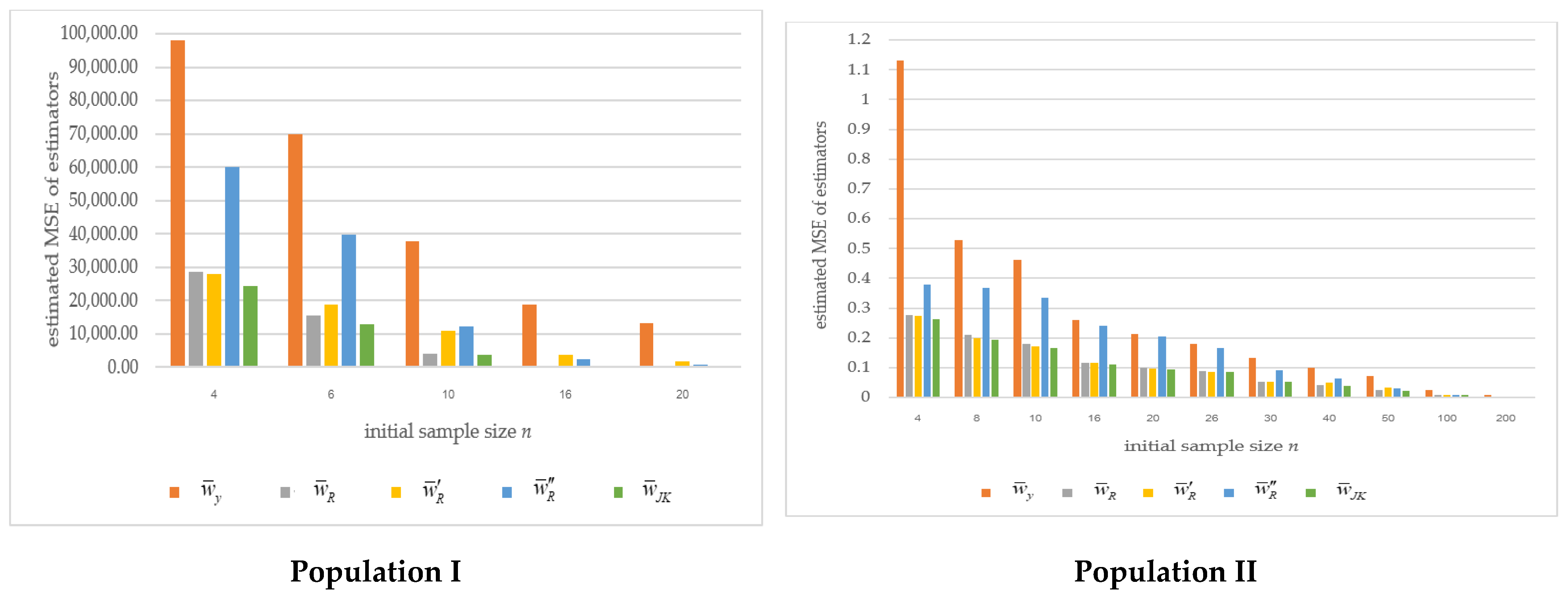
Population I
n	$E\left(\nu \right)$	Estimators without auxiliary variable information		Estimators utilizing auxiliary variable information
		$\overline{y}$	${\overline{w}}_y$	${\overline{w}}_R$	${\overline{w}}_R^{\prime }$	${\overline{w}}_R^{″}$	${\overline{w}}_{JK}$
4	9.6743	460,161.8988	98,093.5592	28,660.4541	28,139.4430	60,246.5137	24,515.0587
8	13.3041	348,211.0954	69,903.2109	15,438.8033	18,899.7352	39,627.6046	12,953.4060
10	18.9176	181,110.7250	37,756.8454	4107.7002	10,795.4605	12,398.3285	3881.9643
16	25.2787	76,613.8482	18,963.6552	533.3519	3771.5275	2526.1157	512.5064
20	28.5644	46,482.3626	13,304.8071	85.8090	1804.1610	763.9441	82.4876
Population II
4	6.8705	10.8216	1.1305	0.2777	0.2730	0.3777	0.2625
8	12.8042	10.8059	0.5291	0.2115	0.1986	0.3679	0.1929
10	15.8498	10.7229	0.4623	0.1792	0.1705	0.3361	0.1649
16	24.8431	9.6113	0.2606	0.1158	0.1149	0.2407	0.1102
20	30.9154	9.2723	0.2122	0.0990	0.0962	0.2040	0.0938
26	38.9001	7.7315	0.1790	0.0873	0.0863	0.1665	0.0856
30	43.8715	6.9521	0.1315	0.0527	0.0521	0.0906	0.0517
40	56.7309	5.9159	0.1004	0.0406	0.0495	0.0651	0.0401
50	68.5383	4.7074	0.0717	0.0252	0.0322	0.0292	0.0215
100	120.1685	1.5727	0.0238	0.0078	0.0091	0.0080	0.0078
200	215.1886	0.2266	0.0076	0.0023	0.0027	0.0024	0.0023

and

Table 3. Relative efficiency of population mean estimators.

Population I
		$\mathrm{RE}\mathrm{of}\mathrm{estimators}\mathrm{compared}\mathrm{with}{\overline{w}}_y$					$\mathrm{RE}\mathrm{of}\mathrm{estimators}\mathrm{compared}\mathrm{with}{\overline{w}}_R$
$n$	$E\left(\nu \right)$	${\overline{w}}_y$	${\overline{w}}_R$	${\overline{w}}_R^{\prime }$	${\overline{w}}_R^{″}$	${\overline{w}}_{JK}$	${\overline{w}}_R$	${\overline{w}}_R^{\prime }$	${\overline{w}}_R^{″}$	${\overline{w}}_{JK}$
4	9.6743	1	3.4226	3.4860	1.6282	4.0014	1	1.0185	0.4757	1.1691
8	13.3041	1	4.5278	3.6986	1.7640	5.3965	1	0.8169	0.3896	1.1919
10	18.9176	1	9.1917	3.4975	3.0453	9.7262	1	0.3805	0.3313	1.0581
16	25.2787	1	35.5556	5.0281	7.5070	37.0018	1	0.1414	0.2111	1.0407
20	28.5644	1	155.0514	7.3745	17.4159	161.2946	1	0.0476	0.1123	1.0403
Population II
4	6.8705	1	4.0712	4.1412	2.9929	4.3076	1	1.0172	0.7352	1.0579
8	12.8042	1	2.5014	2.6639	1.4384	2.7424	1	1.0650	0.5749	1.0964
10	15.8498	1	2.5794	2.7109	1.3755	2.7950	1	1.0510	0.5332	1.0867
16	24.8431	1	2.2500	2.2682	1.0826	2.3652	1	1.0078	0.4811	1.0508
20	30.9154	1	2.1424	2.2061	1.0398	2.2618	1	1.0291	0.4853	1.0554
26	38.9001	1	2.0506	2.0739	1.0754	2.0926	1	1.0116	0.5243	1.0199
30	43.8715	1	2.4950	2.5252	1.4516	2.5452	1	1.0115	0.5817	1.0193
40	56.7309	1	2.4740	2.0307	1.5437	2.5061	1	0.8202	0.6237	1.0125
50	68.5383	1	2.8456	2.2289	2.4582	3.3355	1	0.7826	0.8630	1.1721
100	120.1685	1	3.0606	2.6042	2.9650	3.0606	1	0.8571	0.9750	1.0000
200	215.1886	1	3.2479	2.8464	3.2340	3.2479	1	0.8519	0.9583	1.0000

. Additionally, bar charts in Figure 3 illustrate the behavior of the estimated MSE across various initial sample sizes.

Discussion

Based on the data studied, the variable of interest was positively correlated with the auxiliary variable. The results from the simulation data are presented as follows.

Table 1 presents the estimated absolute relative bias of the biased estimators, namely ${\overline{w}}_R$, ${\overline{w}}_R^{\prime }$, and ${\overline{w}}_{JK}$. For both populations, it can be observed that as the sample size increased, the absolute relative bias for all estimators declined and approached zero.

Table 2 shows that the estimators incorporating auxiliary variable information—given the positive correlation with the variable of interest—consistently yielded lower MSEs than estimators that do not use such information. Notably, ${\overline{w}}_R^{\prime }$ achieved a lower MSE than the traditional ratio estimator ${\overline{w}}_R$ when the initial sample size was small. Among all estimators, ${\overline{w}}_{JK}$ provided the lowest MSE across all initial sample sizes. Although the estimator ${\overline{w}}_R^{″}$ is unbiased, its MSE was higher than that of ${\overline{w}}_R$ despite being lower than that of estimators that do not use auxiliary information. As illustrated in Figure 3, the MSE for all estimators decreased as the sample size increased. Table 3 reports the relative efficiency of each estimator compared with that of ${\overline{w}}_y$ and ${\overline{w}}_R^{\prime }$. Notably, all estimators that incorporate auxiliary variable information demonstrated higher relative efficiency than ${\overline{w}}_y$ across both Population I and Population II. Among them, the estimator ${\overline{w}}_{JK}$ consistently exhibited the highest relative efficiency.

A comparative analysis indicated that both ${\overline{w}}_R^{\prime }$ and ${\overline{w}}_{JK}$ outperformed ${\overline{w}}_R$ in terms of RE, particularly at small to moderate sample sizes. Moreover, as the initial sample size increased, the efficiency of ${\overline{w}}_{JK}$ converged with that of the traditional ratio estimator ${\overline{w}}_R$.

In the case of Population I, while the overall correlation between the auxiliary variable (X) and the variable of interest (Y) was moderate, the correlation between their network-level averages $w_y$ and $w_x$ was substantially higher at 0.99. This strong association accounts for the trends in MSE and relative efficiency (RE) that closely mirror those observed in Population II.

5. Conclusions

Adaptive cluster sampling (ACS) is particularly effective for studying rare and spatially clustered populations. This research proposes three enhanced ratio-type estimators for ACS, building on Chao’s [17] original ratio estimator and employing the jackknife method to reduce bias and improve efficiency. Analytical derivations of bias and MSE were provided for each estimator, and their performance was evaluated through extensive simulation. The simulation results demonstrated that all three proposed estimators outperformed conventional estimators that do not utilize auxiliary variable information. Specifically, ${\overline{w}}_R^{\prime }$ proved to be more efficient than Chao’s estimator for small initial sample sizes, while ${\overline{w}}_{JK}$ exhibited superior efficiency for both small and moderate initial sample sizes. In large-sample settings, the efficiency of ${\overline{w}}_{JK}$ became comparable to that of the traditional ratio estimator. Although ${\overline{w}}_R^{″}$ is an unbiased estimator, its efficiency was the lowest among the estimators that incorporate auxiliary variable information. The practical implications of these findings are particularly relevant for field studies with limited budgets. In such scenarios, the estimators ${\overline{w}}_R^{\prime }$ and ${\overline{w}}_{JK}$ may be the most effective choices because of their superior performance with smaller initial sample sizes. For studies with moderate resource availability requiring a medium-sized initial sample, ${\overline{w}}_{JK}$ continued to demonstrate high efficiency. In cases necessitating a large initial sample size, the ${\overline{w}}_{JK}$ estimator maintained its high efficiency, although its performance became comparable to that of the traditional ratio estimator ${\overline{w}}_R$.

A limitation of the current study lies in the use of a two-group partitioning strategy within the jackknife procedure. The effects of alternative partitioning schemes—such as dividing the sample into three or more groups—have not been explored. Future research could investigate whether multigroup jackknife strategies offer additional improvements in estimator efficiency, particularly in scenarios involving larger sample sizes or more complex population structures. Moreover, this study focused on a single auxiliary variable. Future research could investigate the development of jackknife-based estimators that incorporate multiple auxiliary variables. Such extensions may further improve estimation accuracy, particularly in high-dimensional sampling contexts. Additionally, alternative resampling methods—such as the bootstrap or balanced repeated replication (BRR)—could be explored and compared with the jackknife approach within the framework of adaptive cluster sampling (ACS).

References

- Sisodia, B.V.S.; Dwivedi, V.K.A. Modified ratio Estimator Using Coefficient of Variation of Auxiliary Variable. J. Indian Soc. Agric. Stat. 1981, 33, 13–18. [Google Scholar]
- Singh, H.P.; Tailor, R. Use of Known Correlation Coefficient in Estimating the Finite Population Mean. Stat. Transit. 2003, 6, 553–560. [Google Scholar]
- Yadav, S.K.; Subramani, J.; Mishra, S.S.; Shukla, A.K. Improved Ratio-Cum-Product Estimators of Population Mean Using Known Population Parameters of Auxiliary Variables. Am. J. Oper. Res. 2016, 6, 48–54. [Google Scholar] [CrossRef]
- Jerajuddin, M.; Kishun, J. Modified Ratio Estimators for Population Mean Using Size of the Sample, Selected from Population. Int. J. Sci. Res. Sci. Eng. Technol. 2016, 2, 10–16. [Google Scholar] [CrossRef]
- Soponviwatkul, K.; Lawson, N. New Ratio Estimators for Estimating Population Mean in Simple Random Sampling using a Coefficient of Variation, Correlation Coefficient and a Regression Coefficient. Gazi Univ. J. Sci. 2017, 30, 610–621. [Google Scholar]
- Thompson, S.K. Adaptive cluster sampling. J. Am. Statist. Assoc. 1990, 85, 1050–1059. [Google Scholar] [CrossRef]
- Magnussen, S.; Kurz, W.; Leckie, D.G.; Paradine, D. Adaptive cluster sampling for estimation of deforestation rates. Eur. J. For. Res. 2005, 124, 207–220. [Google Scholar] [CrossRef]
- Noon, B.R.; Ishwar, N.M.; Vasudevan, K. Efficiency of adaptive cluster and random sampling in detecting terrestrial herpetofauna in a tropical rainforest. Wildl. Soc. Bull. 2006, 34, 59–68. [Google Scholar] [CrossRef]
- Sullivan, W.P.; Morrison, B.J.; Beamish, F.W.H. Adaptive cluster sampling: Estimating density of spatially autocorrelated larvae of the sea lamprey with improved precision. J. Great Lakes Res. 2008, 34, 86–97. [Google Scholar] [CrossRef]
- Smith, D.R.; Villella, R.F.; Lemarié, D.P. Application of adaptive cluster sampling to low-density populations of freshwater mussels. Environ. Ecol. Stat. 2003, 10, 7–15. [Google Scholar] [CrossRef]
- Conners, M.E.; Schwager, S.J. The use of adaptive cluster sampling for hydroacoustic surveys. ICES J. Mar. Sci. 2002, 59, 1314–1325. [Google Scholar] [CrossRef]
- Olayiwola, O.M.; Ajayi, A.O.; Onifade, O.C.; Wale-Orojo, O.; Ajibade, B. Adaptive cluster sampling with model based approach for estimating total number of Hidden COVID-19 carriers in Nigeria. Stat. J. IAOS 2020, 36, 103–109. [Google Scholar] [CrossRef]
- Chandra, G.; Tiwari, N.; Nautiyal, R. Adaptive cluster sampling-based design for estimating COVID-19 cases with random samples. Curr. Sci. 2021, 120, 1204–1210. [Google Scholar] [CrossRef]
- Stehlík, M.; Kiseľák, J.; Dinamarca, A.; Alvarado, E.; Plaza, F.; Medina, F.A.; Stehlíková, S.; Marek, J.; Venegas, B.; Gajdoš, A.; et al. REDACS: Regional emergency-driven adaptive cluster sampling for effective COVID-19 management. Stoch. Anal. Appl. 2022, 41, 474–508. [Google Scholar] [CrossRef]
- Hwang, J.; Bose, N.; Fan, S. AUV adaptive sampling methods: A Review. Appl. Sci. 2019, 9, 3145. [Google Scholar] [CrossRef]
- Giouroukis, D.; Dadiani, A.; Traub, J.; Zeuch, S.; Markl, V. A survey of adaptive sampling and filtering algorithms for the internet of things. In Proceedings of the 14th ACM International Conference on Distributed and Event- Based Systems, Montreal, QC, Canada, 13–17 July 2020; pp. 27–38. [Google Scholar] [CrossRef]
- Chao, C.T. Ratio estimation on adaptive cluster sampling. J. Chin. Stat. Assoc. 2004, 42, 307–327. [Google Scholar] [CrossRef]
- Dryver, A.L.; Chao, C.T. Ratio estimators in adaptive cluster sampling. Environmetric 2007, 18, 607–620. [Google Scholar] [CrossRef]
- Chutiman, N.; Kumphon, B. Ratio estimator using two auxiliary variables for adaptive cluster sampling. Thail. Stat. 2008, 6, 241–256. [Google Scholar]
- Chutiman, N. Adaptive cluster sampling using auxiliary variable. J. Math. Stat. 2013, 9, 249–255. [Google Scholar] [CrossRef]
- Yadav, S.K.; Misra, S.; Mishra, S. Efficient estimator for population variance using auxiliary variable. Am. J. Oper. Res. 2016, 6, 9–15. [Google Scholar] [CrossRef]
- Chaudhry, M.S.; Hanif, M. Generalized exponential-cum-exponential estimator in adaptive cluster sampling. Pak. J. Stat. Oper. Res. 2015, 11, 553–574. [Google Scholar] [CrossRef]
- Chaudhry, M.S.; Hanif, M. Generalized difference-cum-exponential estimator in adaptive cluster sampling. Pak. J. Stat. 2017, 33, 335–367. [Google Scholar]
- Bhat, A.A.; Sharma, M.; Shah, M.; Bhat, M. Generalized ratio type estimator under adaptive cluster sampling. J. Sci. Res. 2023, 67, 46–51. [Google Scholar] [CrossRef]
- Thompson, S.K. Sampling, 3rd ed.; John Wiley & Sons, Inc.: Hoboken, NJ, USA, 2012; pp. 319–337. [Google Scholar]
- Banerjie, J.; Tiwari, N. Improved ratio type estimator using jack-knife method of estimation. J. Reliab. Stat. Stud. 2011, 4, 53–63. [Google Scholar]
- Quenouille, M.H. Notes on Bias in Estimation. Biometrika 1956, 43, 353–360. [Google Scholar] [CrossRef]
- Smith, D.R.; Conroy, M.J.; Brakhage, D.H. Efficiency of adaptive cluster sampling for estimating density wintering waterfowl. Biometrics 1995, 51, 777–788. [Google Scholar] [CrossRef]
- Pochai, N. Double and Resampling in Adaptive Cluster Sampling. Doctoral Dissertation, National Institute of Development Administration, Bangkok, Thailand, 2006. [Google Scholar]