Approximated Optimal Solution for Economic Manufacturing Quantity Model

Abstract

This study investigates the use of the bisection algorithm in inventory models to obtain an approximated optimal solution for the economic manufacturing quantity (EMQ) problem under imperfect production conditions. The objectives are threefold. First, we utilize refined estimations of exponential functions to provide tighter lower and upper bounds for the bisection algorithm. Second, we propose three analytical improvements that simplify the solution process, each supported by rigorous proofs. Third, we incorporate recent results from the literature to further enhance the accuracy of exponential function approximations within the EMQ model. Our improved bounding approach significantly reduces the search interval needed by the bisection method and yields an approximate solution that attains a total cost very close to the true optimum. In a numerical example, the proposed method shrinks the initial search range by over 99% compared to prior methods and achieves a production run length that produces a near-minimal average total cost. These findings demonstrate the effectiveness of the enhanced bounds and provide practical insights for inventory models with imperfect processes.

1. Introduction

The optimal production run length is traditionally determined through economic manufacturing quantity (EMQ) models, which assume a perfect and stationary production process. Under this assumption, the system remains stable and continuously produces items that meet quality requirements. However, such an idealized assumption is often unrealistic in practical settings. To address this, several extensions to the traditional EMQ model have been proposed that incorporate imperfect production processes and system deterioration. To address the limitations of traditional EMQ models, Porteus [1] introduced the concept of process deterioration, showing that it is often more economical to produce smaller lot sizes when defects are likely. Rosenblatt and Lee [2] further developed this line of research by assuming that the transition from an in-control to an out-of-control state follows an exponential distribution. Their model demonstrated that when the rate of process deterioration is small, the optimal production run length is shorter than that predicted by classical EMQ models. Subsequent studies have extended these models in various ways. Later works by Hariga and Ben-Daya [3] replaced the exponential assumption with general shift distributions to derive exact solutions. The estimation of exponential functions plays a critical role in determining optimal solutions. Rachamadugu [4] demonstrated the convexity of related cost functions, paving the way for the application of the bisection algorithm. Chung and Lin [5] studied the bisection algorithm for the inventory model with net present value to estimate negative exponential function, and then Chung and Lin [5] tried to find the lower bound and upper bound for positive exponential function. Chung [6] examined the bisection algorithm for the inventory model of Dohi et al. [7]. Chung et al. [8] modified the results of Chung [6], and then Liang et al. [9] provided an improved solution for the open question in Chung et al.’s work [8]. Lan et al. [10] enhanced the upper bound for negative exponential function, and then Yang et al. [11] improved the upper bound for positive exponential function. Lin and Hou [12] extended Rosenblatt and Lee’s model by incorporating restoration costs and imperfect production even in the in-control state. Although their approach provides a pair of bounds to implement the bisection algorithm, there remains room for improvement in terms of precision and convergence— an open problem that has not been resolved in the literature. Our research is aimed at solving this particular problem by providing improved analytical bounds. Lin and Hou [12] provided an upper-bound and lower-bound pair to execute the bisection method to locate the optimal solution. In this study, we present improved pairs of upper bounds and lower bounds to reduce the searching domain to 1%. Moreover, our proposed lower bound attains the minimum value. Our improved bounds significantly reduce the search interval and yield solutions that closely match the optimal production run length. In addition, we provide a closed-form approximation formula that attains the minimum total cost. Our contributions are validated through detailed numerical comparisons with prior models.

Research Objective: The main objective of this research is to develop improved lower-bound and upper-bound functions for the bisection search method in the EMQ model, in order to obtain a more precise approximated optimal solution. We aim to resolve the aforementioned gap by tightening the bounds on the optimal run length and thereby enhancing the accuracy and efficiency of the solution procedure, and then we seek a closed-form approximation of the optimal order quantity for the economic manufacturing quantity model.

Novelty and Contributions: This study offers several novel contributions to the EMQ literature. First, we formulate two refined lower-bound functions and three refined upper-bound functions for the derivative of the total cost function, which dramatically narrows the search interval for locating the optimal production run length. Second, based on these analytical bounds, we propose a new method that finds an approximated optimal run length that achieves the minimum average total cost; this includes providing a closed-form approximate solution for the optimal run length. Third, we present a comprehensive numerical example demonstrating that our improved bounds reduce the initial search range by over 99% compared to Lin and Hou’s approach, thus significantly speeding up convergence to the optimum. Finally, we conduct a sensitivity analysis to offer insights into how key parameters (such as production rate, defect rate, and cost factors) affect the optimal solution, and then we discuss the scope and limitations of the proposed model.

At the time of writing, there are nine papers that have cited Lin and Hou [12] in their references. We examined these nine papers and related papers to discover that they only mention Lin and Hou [12] in their Introduction; as such, we can claim that we are the first paper to provide improvements to the lower and upper bounds for the optimal solution of manufacture run length. We will study the inventory system proposed by Lin and Hou [12] to improve their results for the lower bound and upper bound of the bisection algorithm.

We provide a literature review of economic manufacturing quantity models to indicate the current trends with respect to this hot research topic. With regard to Sustainable Production Inventory Models, Das and Sen [13], Alsaedi [14], Priyan [15], Shahid and Choi [16], Nobil et al. [17], Sivashankari et al. [18], Yee et al. [19], Sebatjane [20,21], Gupta and Khanna [22], and Sivashankari [23] constructed new inventory models to deal with gas emissions and the greenhouse effect. Regarding imperfect production manufacturing problems, Alsaedi [14], Sebatjane [21], Sivashankari [23], Eroğlu and Aydemir [24], Narang and De [25], Utama et al. [26], Hsieh et al. [27], Taleizadeh et al. [28], Deivanayagampillai et al. [29], and Wu et al. [30] developed novel inventory systems to consider rework conditions. Regarding fuzzy inventory models, Alsaedi [14], Priyan [15], Eroğlu and Aydemir [24], Baggiyalakshmi and Maragatham [31], and Wu et al. [32] examined new inventory systems to handle vague environments. Regarding multi-level inventory systems, Hsieh et al. [27], ZolfaghariRazaji et al. [33], Suvetha et al. [34], Malumfashi et al. [35], Madugu et al. [36], Malumfashi et al. [37] and Roy and Ghosh [38] derived solution procedures to locate optimal solutions. Regarding inventory models with stock-dependent demand, Malumfashi et al. [37] and Tshinangi et al. [39] studied their mathematical structure. For inventory systems with time-dependent costs, Gupta et al. [40], Rabiu and Ali [41], and Sivashankari et al. [42] obtained optimal solutions or approximated solutions.

This paper is organized as follows. In Section 1, we review related papers on approximated solutions for this kind of inventory model. In Section 2, we introduce the assumptions and notation. We review previous findings in Section 3. Our improvements are explained in Section 4. To find two lower-bound functions and three upper-bound functions for the objective function, which is related to the first derivative of the average total cost function for inventory model of Rosenblatt and Lee [2] and Lin and Hou [12], we obtain a restriction of $2>x>0$. To derive the desired relationship among these six functions, we improve the criterion to $1>x>0$. To show the abovementioned six functions are all increasing functions, we revise the condition to $\left(2/3\right)>x>0$. We provide a numerical example in Section 5 with detailed comparison with different approximated solutions. Moreover, we present graphs to visualize our analytic results. In Section 6, we construct a formulated approximated optimal solution that also attains the minimum value. We produce a sensitivity analysis with graphical explanations in Section 7. We discuss contributions and limitations in Section 8. Finally, we conclude our study in Section 9 and indicate that our approximated solutions are very close to the genuine optimal solution, such that our proposed lower bound, upper bound, and formulated approximated solutions all attain the minimum value.

2. Assumptions and Notation

For convenience, we use the same notation and assumptions as Rosenblatt and Lee [2] and Lin and Hou [12]:

(A) It is supposed that all the items produced are ready and can be classified as being either conforming or nonconforming, depending on whether their performance meets the products’ requirements or not.

(B) Due to production inconsistency, an item is nonconforming with probability ${\mathsf{\theta }}_1$ (or ${\mathsf{\theta }}_2$) when the production procedure is in control (or out of control), where ${\mathsf{\theta }}_1<{\mathsf{\theta }}_2$.

(C) If the system is in an out-of-control state, it can be repaired to an in-control state with modifications or restoration cost, denoted as $\mathrm{r}$, with $\mathrm{r}>0$ for the next manufacture run.

(D) The nonconforming items will finally be reworked with cost $\mathrm{s}$ so that the function of the production system will be unaffected.

(E) After a manufacture run, the system is set up with cost, denoted as $\mathrm{k}$, with $\mathrm{k}>0$, and is inspected to disclose the state of the system.

(F) Assume that the inventory carrying cost for holding an item per unit time is denoted as $\mathrm{h}$.

(G) Assume that the manufacture rate of the model and the demand rate of the product are denoted as $\mathrm{p}$ and $\mathrm{d}$, respectively, where $\mathrm{p}>\mathrm{d}$.

(H) Given that the manufacture run length is $\mathrm{t}$, the time span of a manufacture cycle $\mathrm{T}$ satisfies the relation $\mathrm{d}\mathrm{T}=\mathrm{p}\mathrm{t}$, and the maximum inventory level is expressed as $\left(\mathrm{p}-\mathrm{d}\right)\mathrm{t}$.

(I) Lin and Hou [12] declared the deterioration of the production process by assuming a shift from an “in-control” to an “out-of-control” state, where the elapsed time of the system in an in-control state follows an exponential distribution with finite mean $1/\mathsf{\lambda }$.

(J) $\mathsf{\beta }=\left(\mathrm{d}\mathrm{r}/\mathrm{p}\right)+\left[\mathrm{d}\mathrm{s}\left({\mathsf{\theta }}_1-{\mathsf{\theta }}_2\right)/\mathsf{\lambda }\right]$ is an abbreviation to simplify the expression.

Moreover, we provide a list of notations to indicate the symbols and variables that are used in the model:

$\mathrm{d}$: demand rate of the product (units per unit time);

$\mathrm{h}$: inventory holding cost (per item per unit time);

$\mathrm{k}$: setup cost incurred for each production run (setup and inspection cost);

$\mathrm{p}$: production rate (units produced per unit time);

$\mathrm{r}$: restoration cost to repair the system after an out-of-control state (per occurrence);

$\mathrm{s}$: cost to rework each nonconforming (defective) item;

$\mathrm{t}$: production run length (decision variable);

$\mathrm{T}$: length of a complete production-inventory cycle.

Since Rosenblatt and Lee [2] studied first economic manufacturing quantity models, there have been eighty-five papers that have referenced this study, such that many extensions in several aspects have been improved and continuously revolved. Lin and Hou [12] provide an important further study of Rosenblatt and Lee [2]. The motivation of this paper is to present an improved pair of lower and upper bounds for the optimal solution with respect to Lin and Hou [12].

3. Overview of Previous Findings

Lin and Hou [12] considered the restoration cost and the probability of nonconforming items during the in-control production procedure, such that they extended the economic manufacturing quantity model to derive the expected total cost per unit time, $\mathrm{T}\mathrm{C}\left(\mathrm{t}\right)$, as follows:

$$\mathrm{T}\mathrm{C}\left(\mathrm{t}\right)=\left(\mathrm{d}\mathrm{k}/\mathrm{p}\mathrm{t}\right)+\left[\mathrm{h}\left(\mathrm{p}-\mathrm{d}\right)\mathrm{t}/2\right]+\mathrm{d}\mathrm{s}{\mathsf{\theta }}_2+\left[\mathsf{\beta }\left(1-{\mathrm{e}}^{-\mathsf{\lambda }\mathrm{t}}\right)/\mathrm{t}\right],$$

(1)

with the following abbreviation:

$$\mathsf{\beta }=\left(\mathrm{d}\mathrm{r}/\mathrm{p}\right)+\left[\mathrm{d}\mathrm{s}\left({\mathsf{\theta }}_1-{\mathsf{\theta }}_2\right)/\mathsf{\lambda }\right].$$

(2)

For a given production run length, $\mathrm{t}$, Equation (1) represents the average total cost per unit time. The optimization problem involves determining the value of t, with the restriction $\mathrm{t}>0$, which minimizes this cost function under the condition $\mathrm{p}>\mathrm{d}$.

They found that

$$\mathrm{d}\mathrm{T}\mathrm{C}\left(\mathrm{t}\right)/\mathrm{d}\mathrm{t}=\left\{\left[\mathrm{h}\left(\mathrm{p}-\mathrm{d}\right){\mathrm{t}}^2/2\right]-\left(\mathrm{d}\mathrm{k}/\mathrm{p}\right)+\mathsf{\beta }\left[\left(1+\mathsf{\lambda }\mathrm{t}\right){\mathrm{e}}^{-\mathsf{\lambda }\mathrm{t}}-1\right]\right\}/{\mathrm{t}}^2.$$

(3)

To simplify the expression, Lin and Hou [17] assumed an auxiliary function, denoted as $\mathrm{f}\left(\mathrm{t}\right)$, as follows:

$$\mathrm{f}\left(\mathrm{t}\right)=\left[\mathrm{h}\left(\mathrm{p}-\mathrm{d}\right){\mathrm{t}}^2/2\right]-\left(\mathrm{d}\mathrm{k}/\mathrm{p}\right)+\mathsf{\beta }\left[\left(1+\mathsf{\lambda }\mathrm{t}\right){\mathrm{e}}^{-\mathsf{\lambda }\mathrm{t}}-1\right].$$

(4)

To locate the optimal solution, that is, the solution of $\mathrm{f}\left(\mathrm{t}\right)=0$, Lin and Hou [12] tried to find two approximations for

$$\left(1+\mathrm{x}\right){\mathrm{e}}^{-\mathrm{x}}-1,$$

(5)

such that they could locate an upper bound and a lower bound to execute the bisection algorithm to locate the optimal solution. Lin and Hou [12] assumed that

$${\mathrm{t}}_1=\sqrt{2\mathrm{d}\mathrm{k}/\mathrm{h}\mathrm{p}\left(\mathrm{p}-\mathrm{d}\right)},$$

(6)

and

$${\mathrm{t}}_2=\sqrt{2\mathrm{d}\mathrm{k}/\left[\mathrm{h}\mathrm{p}\left(\mathrm{p}-\mathrm{d}\right)-\mathrm{p}\mathsf{\beta }{\mathsf{\lambda }}^2\right]},$$

(7)

with ${\mathrm{t}}^{\ast }$ being the optimal solution. We quote their main results in the following:

Proposition 2 of Lin and Hou [12]: If $\mathsf{\beta }\le 0$, then $0<{\mathrm{t}}^{\ast }\le {\mathrm{t}}_1$, and if $\mathsf{\beta }>0$, then ${\mathrm{t}}_1<{\mathrm{t}}^{\ast }<{\mathrm{t}}_2$.

We will offer our improvements for lower and upper bounds with the bisection algorithm proposed by Lin and Hou [12].

4. Our Improvement

To simplify the expression, we will use $\mathrm{x}=\mathsf{\lambda }\mathrm{t}$ as the new variable.

From the numerical example of Lin and Hou [12], we know that

$$\mathrm{d}\mathrm{r}/\mathrm{p}=1.33\times {10}^2,$$

(8)

and

$$\mathrm{d}\mathrm{s}\left({\mathsf{\theta }}_1-{\mathsf{\theta }}_2\right)/\mathsf{\lambda }=-8.12\times {10}^4,$$

(9)

such that

$$\mathsf{\beta }=-8.11\times {10}^4.$$

(10)

Hence, without a loss of generality, we claim the following observation:

Observation 1.

We will explain that from a practical point of view,   $\beta$ is negative, where   $\beta =\left(dr/p\right)+\left[ds\left({\theta }_1-{\theta }_2\right)/\lambda \right]$ is defined by Equation (2) of Lin and Hou [12].

According to Observation 1, in the rest of this paper, we will assume that $\mathsf{\beta }<0$. Now, we recall the estimation for the negative exponential function. Chung and Lin [5] estimated ${\mathrm{e}}^{-\mathrm{x}}$; for $\mathrm{x}>0$,

$$1-\mathrm{x}+\left({\mathrm{x}}^2/2\right)>{\mathrm{e}}^{-\mathrm{x}}>\left[\left(2-\mathrm{x}\right)/\left(2+\mathrm{x}\right)\right].$$

(11)

Lan et al. [10] obtained that for $\mathrm{x}>0$,

$$\left[\left(6-4\mathrm{x}+{\mathrm{x}}^2\right)/\left(6+2\mathrm{x}\right)\right]>{\mathrm{e}}^{-\mathrm{x}}>\left[\left(2-\mathrm{x}\right)/\left(2+\mathrm{x}\right)\right].$$

(12)

Yang et al. [11] showed that for $2>x>0$,

$$\left[\left(2+\mathrm{x}\right)/\left(2-\mathrm{x}\right)\right]\ge \left[\left(6+4\mathrm{x}+{\mathrm{x}}^2\right)/\left(6-2\mathrm{x}\right)\right]\ge {\mathrm{e}}^{\mathrm{x}}.$$

(13)

Consequently, taking the reciprocal of Equation (13), it yields that for $2>x>0$,

$${\mathrm{e}}^{-\mathrm{x}}\ge \left[\left(6-2\mathrm{x}\right)/\left(6+4\mathrm{x}+{\mathrm{x}}^2\right)\right]\ge \left[\left(2-\mathrm{x}\right)/\left(2+\mathrm{x}\right)\right].$$

(14)

Based on the above discussion, we will derive several lower bounds and upper bounds for the bisection algorithm proposed by Lin and Hou [12].

To estimate $\left(1+\mathrm{x}\right){\mathrm{e}}^{-\mathrm{x}}-1$ of Equation (5), Lin and Hou [12] derived that

$$0>\left(1+\mathrm{x}\right){\mathrm{e}}^{-\mathrm{x}}-1.$$

(15)

According to the estimation from Chung and Lin [5] of Equation (11), we can imply that for $2>x>0$,

$$\left[\left({\mathrm{x}}^3-{\mathrm{x}}^2\right)/2\right]>\left(1+\mathrm{x}\right){\mathrm{e}}^{-\mathrm{x}}-1>\left[-{\mathrm{x}}^2/\left(2+\mathrm{x}\right)\right].$$

(16)

Based on Equation (12) proposed by Lan et al. [10], for $2>x>0$,

$$\left[\left({\mathrm{x}}^3-3{\mathrm{x}}^2\right)/\left(6+2\mathrm{x}\right)\right]>\left(1+\mathrm{x}\right){\mathrm{e}}^{-\mathrm{x}}-1>\left[-{\mathrm{x}}^2/\left(2+\mathrm{x}\right)\right].$$

(17)

Owing to the results of the first inequality in Equation (14), which was based on Equation (13) proposed by Yang et al. [11], we imply that for $2>x>0$,

$$\left(1+\mathrm{x}\right){\mathrm{e}}^{-\mathrm{x}}-1>\left[-3{\mathrm{x}}^2/\left(6+4\mathrm{x}+{\mathrm{x}}^2\right)\right].$$

(18)

There is no upper-bound function in Yang et al.’s work [11]. If we try to execute the bisection method, then we will apply the upper bound of Equation (17) as the proposed upper bound. We will use the above results of Equations (16)–(18) to locate improved lower bounds and upper bounds for the bisection algorithm.

For the relations mentioned in Equation (16), the restriction for the variable x is $2>x>0$. In the following, we will explain how to establish the new relations in Equation (19), such that we must revise the condition from $2>x>0$ to $1>x>0$.

For $2>\mathrm{x}>0$, we will find a reasonable condition, such as $0<x<1$, to show that

$$0>{\displaystyle \frac{{\mathrm{x}}^3-{\mathrm{x}}^2}{2}}>{\displaystyle \frac{{\mathrm{x}}^3-3{\mathrm{x}}^2}{6+2\mathrm{x}}}>\left(1+\mathrm{x}\right){\mathrm{e}}^{-\mathrm{x}}-1>{\displaystyle \frac{-3{\mathrm{x}}^2}{6+4\mathrm{x}+{\mathrm{x}}^2}}>{\displaystyle \frac{-{\mathrm{x}}^2}{2+\mathrm{x}}}.$$

(19)

The condition to ensure the first inequality in Equation (19) is $0<x<1$. This is the reason why we need to modify the range from $2>\mathrm{x}>0$, of Equations (16)–(18), to

$$1>x>0.$$

(20)

To verify the second inequality in Equation (19),

$$2{\mathrm{x}}^4+2{\mathrm{x}}^3>0.$$

(21)

Hence, there is no extra condition to guarantee the validation of Equation (21).

The assertion of the third inequality in Equation (19) is already discussed by Lin and Hou [12], as we mentioned with regard to Equation (17).

The fourth inequality in Equation (19) is already discussed in Equation (18).

The condition to ensure the fifth inequality in Equation (19) is

$$6+3\mathrm{x}<6+4x+{\mathrm{x}}^2.$$

(22)

Hence, there is no extra condition to guarantee the validation of Equation (22). We summarize our findings in the next theorem.

Theorem 1.

For   $x$ with   $0<x<1$, then

$$0>{\displaystyle \frac{{\mathrm{x}}^3-3{\mathrm{x}}^2}{2}}>{\displaystyle \frac{{\mathrm{x}}^3-3{\mathrm{x}}^2}{6+2\mathrm{x}}}>\left(1+\mathrm{x}\right){\mathrm{e}}^{-\mathrm{x}}-1>{\displaystyle \frac{-3{\mathrm{x}}^2}{6+4\mathrm{x}+{\mathrm{x}}^2}}>{\displaystyle \frac{-{\mathrm{x}}^2}{2+\mathrm{x}.}}$$

For further discussion under the restriction of $0<x<1$, as mentioned in Theorem 1, we assume the following five auxiliary functions, with the objective function $\mathrm{f}\left(\mathrm{t}\right)$ of Equation (4) in the variable of $\mathrm{x}$, to obtain two lower bounds and three upper bounds for the bisection method to locate the optimal solution of $\mathrm{d}\mathrm{T}\mathrm{C}\left(\mathrm{t}\right)/\mathrm{d}\mathrm{t}=0$.

Under the restriction of $0<x<1$, we assume that

$${\mathrm{L}\mathrm{B}}_2\left(\mathrm{x}\right)=\left[\mathrm{h}\left(\mathrm{p}-\mathrm{d}\right){\mathrm{x}}^2/2{\mathsf{\lambda }}^2\right]-\left(\mathrm{d}\mathrm{k}/\mathrm{p}\right)+\mathsf{\beta }\left[-{\mathrm{x}}^2/\left(2+\mathrm{x}\right)\right].$$

(23)

$${\mathrm{L}\mathrm{B}}_1\left(\mathrm{x}\right)=\left[\mathrm{h}\left(\mathrm{p}-\mathrm{d}\right){\mathrm{x}}^2/2{\mathsf{\lambda }}^2\right]-\left(\mathrm{d}\mathrm{k}/\mathrm{p}\right)+\mathsf{\beta }\left[-3{\mathrm{x}}^2/\left(6+4\mathrm{x}+{\mathrm{x}}^2\right)\right].$$

(24)

$$\mathrm{f}\left(\mathrm{x}\right)=\left[\mathrm{h}\left(\mathrm{p}-\mathrm{d}\right){\mathrm{x}}^2/2{\mathsf{\lambda }}^2\right]-\left(\mathrm{d}\mathrm{k}/\mathrm{p}\right)+\mathsf{\beta }\left[\left(1+\mathrm{x}\right){\mathrm{e}}^{-\mathrm{x}}-1\right].$$

(25)

$${\mathrm{U}\mathrm{B}}_1\left(\mathrm{x}\right)=\left[\mathrm{h}\left(\mathrm{p}-\mathrm{d}\right){\mathrm{x}}^2/2{\mathsf{\lambda }}^2\right]-\left(\mathrm{d}\mathrm{k}/\mathrm{p}\right)+\mathsf{\beta }\left[\left({\mathrm{x}}^3-3{\mathrm{x}}^2\right)/\left(6+2\mathrm{x}\right)\right].$$

(26)

$${\mathrm{U}\mathrm{B}}_2\left(\mathrm{x}\right)=\left[\mathrm{h}\left(\mathrm{p}-\mathrm{d}\right){\mathrm{x}}^2/2{\mathsf{\lambda }}^2\right]-\left(\mathrm{d}\mathrm{k}/\mathrm{p}\right)+\mathsf{\beta }\left[\left({\mathrm{x}}^3-{\mathrm{x}}^2\right)/2\right].$$

(27)

and

$${\mathrm{U}\mathrm{B}}_3\left(\mathrm{x}\right)=\left[\mathrm{h}\left(\mathrm{p}-\mathrm{d}\right){\mathrm{x}}^2/2{\mathsf{\lambda }}^2\right]-\left(\mathrm{d}\mathrm{k}/\mathrm{p}\right).$$

(28)

We will prove that ${\mathrm{L}\mathrm{B}}_{\mathrm{j}}\left(\mathrm{x}\right)$, for $\mathrm{j}=1,2$, $\mathrm{f}\left(\mathrm{x}\right)$, and ${\mathrm{U}\mathrm{B}}_{\mathrm{k}}\left(\mathrm{x}\right)$ for $\mathrm{k}=1,2,3$ are all increasing functions, such that ${\mathrm{L}\mathrm{B}}_{\mathrm{j}}\left(\mathrm{x}\right)=0$ has a solution ${\mathrm{x}}_{\mathrm{L}\mathrm{B}}\left(\mathrm{j}\right)$ for $\mathrm{j}=1,2$ and ${\mathrm{U}\mathrm{B}}_{\mathrm{k}}\left(\mathrm{x}\right)=0$, for $\mathrm{k}=1,2,3$ has a solution ${\mathrm{x}}_{\mathrm{U}\mathrm{B}}\left(\mathrm{k}\right)$ for $\mathrm{k}=1,2,3$. To prove the increasing property of our six studied functions, we need to further improve the restriction from $1>x>0$ to $2/3>x>0$.

We indicate that ${\mathrm{x}}_{\mathrm{U}\mathrm{B}}\left(3\right)=\mathsf{\lambda }{\mathrm{t}}_1$, where ${\mathrm{t}}_1$ is defined in Equation (6) by Lin and Hou [12].

In the following, we will prove that

$$0<{\mathrm{x}}_{\mathrm{L}\mathrm{B}}\left(2\right)<{\mathrm{x}}_{\mathrm{L}\mathrm{B}}\left(1\right)<{\mathrm{x}}^{\ast }<{\mathrm{x}}_{\mathrm{U}\mathrm{B}}\left(1\right)<{\mathrm{x}}_{\mathrm{U}\mathrm{B}}\left(2\right)<{\mathrm{x}}_{\mathrm{U}\mathrm{B}}\left(3\right),$$

(29)

under a further restriction of $0<x<2/3$.

Theorem 2.

Under the condition of   $0<x<2/3$, we claim that   ${LB}_j\left(x\right)$ for   $j=1,2$,   $f\left(x\right)$ and   ${UB}_k\left(x\right)$ for   $k=1,2,3$ are all increasing functions.

Proof of Theorem 2.

The purpose of proving the increasing property for the examined six functions is to guarantee that there is only one zero for those six functions, such that the well-defined problem for the six zeros is proved.

It is trivial that ${\mathrm{U}\mathrm{B}}_3\left(\mathrm{x}\right)$ is an increasing function for $\mathrm{x}>0$, because ${\mathrm{U}\mathrm{B}}_3\left(\mathrm{x}\right)=\left[\mathrm{h}\left(\mathrm{p}-\mathrm{d}\right){\mathrm{x}}^2/2{\mathsf{\lambda }}^2\right]-\left(\mathrm{d}\mathrm{k}/\mathrm{p}\right)$ is a quadratic function without the linear term.

Since

$${\mathrm{d}\mathrm{U}\mathrm{B}}_2\left(\mathrm{x}\right)/\mathrm{d}\mathrm{x}=\left[\mathrm{h}\left(\mathrm{p}-\mathrm{d}\right)\mathrm{x}/{\mathsf{\lambda }}^2\right]+\mathrm{x}\mathsf{\beta }\left[\left(3\mathrm{x}/2\right)-1\right].$$

(30)

to ensure

$${\mathrm{d}\mathrm{U}\mathrm{B}}_2\left(\mathrm{x}\right)/\mathrm{d}\mathrm{x}>0,$$

(31)

owing to $\mathsf{\beta }<0$, we require another constraint:

$$\left(3\mathrm{x}/2\right)-1<0.$$

(32)

This is the exact reason why we restrict the range from $1>x>0$ to

$$\left(2/3\right)>x>0.$$

(33)

From

$${\mathrm{d}\mathrm{U}\mathrm{B}}_1\left(\mathrm{x}\right)/\mathrm{d}\mathrm{x}=\left[\mathrm{h}\left(\mathrm{p}-\mathrm{d}\right)\mathrm{x}/{\mathsf{\lambda }}^2\right]+4\mathrm{x}\mathsf{\beta }\left[\left({\mathrm{x}}^2+6\mathrm{x}-9\right)/{\left(6+2\mathrm{x}\right)}^2\right],$$

(34)

for $1>x>0$, we recall that $\mathsf{\beta }<0$. It follows that in the domain of $1>x>0$,

$${\mathrm{x}}^2+6\mathrm{x}-9<0,$$

(35)

is valid. Thus, there is no extra condition needed to guarantee that

$${\mathrm{d}\mathrm{U}\mathrm{B}}_1\left(\mathrm{x}\right)/\mathrm{d}\mathrm{x}>0.$$

(36)

$\mathrm{f}\left(\mathrm{x}\right)$ is an increasing function, already discussed in Appendix I of Lin and Hou [12].

By

$${\mathrm{d}\mathrm{L}\mathrm{B}}_1\left(\mathrm{x}\right)/\mathrm{d}\mathrm{x}=\left[\mathrm{h}\left(\mathrm{p}-\mathrm{d}\right)\mathrm{x}/{\mathsf{\lambda }}^2\right]-12\mathsf{\beta }\mathrm{x}\left[\left(3+\mathrm{x}\right)/{\left(6+4\mathrm{x}+{\mathrm{x}}^2\right)}^2\right],$$

(37)

and

$${\mathrm{d}\mathrm{L}\mathrm{B}}_2\left(\mathrm{x}\right)/\mathrm{d}\mathrm{x}=\left[\mathrm{h}\left(\mathrm{p}-\mathrm{d}\right)\mathrm{x}/{\mathsf{\lambda }}^2\right]-\mathsf{\beta }\mathrm{x}\left[\left(4+\mathrm{x}\right)/{\left(2+\mathrm{x}\right)}^2\right],$$

(38)

with Observation 1, we know that $\mathsf{\beta }<0$. Hence, we obtain that ${\mathrm{d}\mathrm{L}\mathrm{B}}_{\mathrm{j}}\left(\mathrm{x}\right)/\mathrm{d}\mathrm{x}>0$ for $\mathrm{j}=1,2$ with $\mathrm{x}>0$. □

In the following, we will explain that the restriction of $3\mathrm{x}<2$ will be held from the practical point of view. From the numerical example, we know that $\mathsf{\lambda }=0.2$ under the constraint of $3\mathrm{x}<2$, which means that $\mathrm{t}<\left(2/3\mathsf{\lambda }\right)=10/3$ years, i.e., that we will find the optimal production length within three years and four months. Compared to the optimal production length of three months in the numerical example, our constraint of three years and four months is a big enough range to cover the possible solution. Hence, we conclude the following observation:

Observation 2.

The constraint of $3x=3\lambda t<2$ is a reasonable condition.

The increasing property of the six functions of Equations (23)–(28) yields the uniqueness of the root. To verify the existence of the root, we need another observation on the magnitude of $\mathsf{\lambda }{\mathrm{t}}_1$.

From the numerical example of Lin and Hou [12], we know that

$$\mathsf{\lambda }{\mathrm{t}}_1\approx 0.1,$$

(39)

Hence, we say that without loss of generality,

$$\mathsf{\lambda }{\mathrm{t}}_1<2/3.$$

(40)

Based on our discussion of Equations (39) and (40), we conclude the following observation:

Observation 3.

We show that, from a practical point of view,

$$\mathsf{\lambda }{\mathrm{t}}_1=\mathsf{\lambda }\sqrt{2\mathrm{d}\mathrm{k}/\mathrm{h}\mathrm{p}\left(\mathrm{p}-\mathrm{d}\right)}<2/3.$$

(41)

According to Observation 3, we accept that

$${\mathrm{x}}_{\mathrm{U}\mathrm{B}}\left(3\right)=\mathsf{\lambda }{\mathrm{t}}_1<2/3,$$

(42)

is an acceptable condition. From Observation 1, Theorem 1, and Equations (23)–(28), we imply that for $\left(2/3\right)>x>0$,

$${\mathrm{L}\mathrm{B}}_2\left(\mathrm{x}\right)>{\mathrm{L}\mathrm{B}}_1\left(\mathrm{x}\right)>f\left(\mathrm{x}\right)>{\mathrm{U}\mathrm{B}}_1\left(\mathrm{x}\right)>{\mathrm{U}\mathrm{B}}_2\left(\mathrm{x}\right)>{\mathrm{U}\mathrm{B}}_3\left(\mathrm{x}\right).$$

(43)

From the Intermediate Value Theorem and Theorem 2, there are unique roots for the four auxiliary functions defined by Equations (23), (24), (26), and (27) with the goal function $\mathrm{f}\left(\mathrm{x}\right)$ of Equation (25). Again, using Equation (43), it follows that

$$0<{\mathrm{x}}_{\mathrm{L}\mathrm{B}}\left(2\right)<{\mathrm{x}}_{\mathrm{L}\mathrm{B}}\left(1\right)<{\mathrm{x}}^{\ast }<{\mathrm{x}}_{\mathrm{U}\mathrm{B}}\left(1\right)<{\mathrm{x}}_{\mathrm{U}\mathrm{B}}\left(2\right)<{\mathrm{x}}_{\mathrm{U}\mathrm{B}}\left(3\right).$$

(44)

These refined bounds pave the way for the efficient computation of the optimal run length, as illustrated in the numerical experiments below.

According to Equation (44), we provide two improved lower bounds and two revised upper bounds where ${\mathrm{x}}_{\mathrm{U}\mathrm{B}}\left(3\right)=\mathsf{\lambda }{\mathrm{t}}_1$, as already discovered by Lin and Hou [12]. In the numerical example, we will illustrate that our lower bounds and upper bounds are very accurate, such that they will attain the minimum solution.

5. Numerical Example

To illustrate that our finding is compatible with Lin and Hou [12], we consider the same numerical example as Lin and Hou [12] with the following data: $\mathrm{d}=1000$ unit/year, $\mathrm{p}=1500$ unit/year, $\mathrm{k}=200$$, $\mathrm{r}=200$$, $\mathsf{\lambda }=0.2$ 1/year, $\mathrm{h}=2$$/unit · year, $\mathrm{s}=25$$/unit, ${\mathsf{\theta }}_1=0.1$, and ${\mathsf{\theta }}_2=0.75$. For clarity and consistency, we adopt the same numerical example as used in Lin and Hou [12]. This allows a direct comparison of our improved approach with the original results under identical conditions.

This implies that $\mathsf{\beta }=-8.11\times {10}^4<0$; Lin and Hou [12] found the lower bound, $0$, and upper bound, ${\mathrm{x}}_{\mathrm{U}\mathrm{B}}\left(3\right)/\mathsf{\lambda }=0.516398$. Using the results of Equation (44), we obtain two lower bounds as

$${\mathrm{x}}_{\mathrm{L}\mathrm{B}}\left(2\right)/\mathsf{\lambda }=0.253045<{\mathrm{x}}_{\mathrm{L}\mathrm{B}}\left(1\right)/\mathsf{\lambda }=0.253884<{\mathrm{t}}^{\ast }=0.253891,$$

(45)

and two upper bounds as

$${\mathrm{t}}^{\ast }=0.253891<{\mathrm{x}}_{\mathrm{U}\mathrm{B}}\left(1\right)/\mathsf{\lambda }=0.253898<{\mathrm{x}}_{\mathrm{U}\mathrm{B}}\left(2\right)/\mathsf{\lambda }=0.255695.$$

(46)

We list the relative ratios among the ranges of the upper bounds and lower bounds for different approaches in the next table, where the base is the results of Lin and Hou [12].

From

Table 1. Starting points for the bisection algorithm under different bounds.

Source	Lower Bound	Upper Bound	Range Ratio
Lin and Hou [12]	$0$	$0.516398$	$1$
Chung and Lin [5]	$0.253045$	$0.255695$	$5.1\times {10}^{-3}$
Lan et al. [10]	$0.253045$	$0.253898$	$1.7\times {10}^{-3}$
Yang et al. [11]	$0.253884$	$0.253898$	$2.7\times {10}^{-5}$

, if we apply the results of Chung and Lin [5], then the range can shrink to $0.51\%$. If we use the results of Lan et al. [10], then the range is even smaller at $0.17\%$. Finally, if we employ the findings of Yang et al. [11], then the range can be minimized to $0.003\%$. This indicates that our lower bounds and upper bounds are very close, such that our results dramatically improve the results of Lin and Hou [12]. Moreover, we will compare the total cost among the starting lower bounds and upper bounds with the minimum values in

Table 2. The total cost evaluated at each starting point.

Source	Total Cost at the Beginning: Lower Bound	Total Cost at the Beginning: Upper Bound
Lin and Hou [12]	$1.33\times {10}^8$	$3852.722$
Chung and Lin [5]	$3583.789$	$3583.810$
Lan et al. [10]	$3583.789$	$3583.784$
Yang et al. [11]	$3583.784$	$3583.784$

.

If we examine the total costs listed in Table 2 with the optimal manufacture run length of

$${\mathrm{t}}^{\ast }=0.253891,$$

(47)

and

$$\mathrm{T}\mathrm{C}\left({\mathrm{t}}^{\ast }\right)=3583.784,$$

(48)

then using the results of Yang et al. [11], both the lower bound and the upper bound attained the minimum value. The beginning upper bound and lower bound of Lin and Hou [12] are far away from the minimum value. Our enhanced lower bound dramatically improves the value of the total cost. Moreover, Lan et al. [10] also provided a very closed estimation for the minimum value.

For completeness, we present the following examination of the bisection method with a starting pair of lower and upper bounds, as mentioned in Table 1. With the starting lower bound, denoted as ${\mathrm{L}}_1$, and the starting upper bound, denoted as ${\mathrm{U}}_1$, we then define the middle point, denoted as ${\mathrm{M}}_{\mathrm{k}}=\left({\mathrm{L}}_{\mathrm{k}}+{\mathrm{U}}_{\mathrm{k}}\right)/2$, for $\mathrm{k}=1,2,\dots$. We check the value of $\mathrm{f}\left({\mathrm{M}}_{\mathrm{k}}\right)$ to decide the choice of ${\mathrm{L}}_{\mathrm{k}+1}$ and ${\mathrm{U}}_{\mathrm{k}+1}$, $\mathrm{k}=1,2,\dots$, using the following rules:

(i).

If $\mathrm{f}\left({\mathrm{M}}_{\mathrm{k}}\right)=0$, then we derive that ${\mathrm{t}}^{\ast }={\mathrm{M}}_{\mathrm{k}}$;

(ii).

If $\mathrm{f}\left({\mathrm{M}}_{\mathrm{k}}\right)<0$, then we define that ${\mathrm{L}}_{\mathrm{k}+1}={\mathrm{M}}_{\mathrm{k}}$ and ${\mathrm{U}}_{\mathrm{k}+1}={\mathrm{U}}_{\mathrm{k}}$;

(iii).

If $\mathrm{f}\left({\mathrm{M}}_{\mathrm{k}}\right)>0$, then we define that ${\mathrm{L}}_{\mathrm{k}+1}={\mathrm{L}}_{\mathrm{k}}$ and ${\mathrm{U}}_{\mathrm{k}+1}={\mathrm{M}}_{\mathrm{k}}$.

These rules apply for $\mathrm{k}=1,2,\dots$.

If $\left|{\mathrm{M}}_{\mathrm{k}}-{\mathrm{M}}_{\mathrm{k}+1}\right|$ is less than a pre-designed threshold, then we stop the bisection algorithm. In this paper, the pre-designed threshold is $1\times {10}^{-3}$.

We run the bisection method for the starting pair proposed by Lin and Hou [12], as expressed in the second row of Table 1, and then we list the computation results of the sequence $\left({\mathrm{M}}_{\mathrm{k}}\right)$ for $\mathrm{k}=1,2,\dots$. We derive that ${\mathrm{M}}_1=0.258199$, ${\mathrm{M}}_2=0.129100$, ${\mathrm{M}}_3=0.193649$, ${\mathrm{M}}_4=0.225924$, ${\mathrm{M}}_5=0.242062$, ${\mathrm{M}}_6=0.250130$, ${\mathrm{M}}_7=0.254165$, ${\mathrm{M}}_8=0.252148$, ${\mathrm{M}}_9=0.253156$, ${\mathrm{M}}_{10}=0.253660$, ${\mathrm{M}}_{11}=0.253913$, ${\mathrm{M}}_{12}=0.253786$, ${\mathrm{M}}_{13}=0.253850$, ${\mathrm{M}}_{14}=0.253881$, ${\mathrm{M}}_{15}=0.253897$, ${\mathrm{M}}_{16}=0.253889$, ${\mathrm{M}}_{17}=0.253893$, and ${\mathrm{M}}_{18}=0.253891={\mathrm{t}}^{\ast }$. Hence, the iterative procedure needs eighteen steps for the bisection method with the starting pair proposed by Lin and Hou [12].

We perform the bisection method for the starting pair proposed by Chung and Lin [5], as expressed in the third row of Table 1, and then we list the computation results of the sequence $\left({\mathrm{M}}_{\mathrm{k}}\right)$ for $\mathrm{k}=1,2,\dots$. We obtain that ${\mathrm{M}}_1=0.254371$, ${\mathrm{M}}_2=0.253908$, ${\mathrm{M}}_3=0.254039$, ${\mathrm{M}}_4=0.253873$, ${\mathrm{M}}_5=0.253956$, ${\mathrm{M}}_6=0.253915$, ${\mathrm{M}}_7=0.253894$, ${\mathrm{M}}_8=0.253884$, ${\mathrm{M}}_9=0.253889$, ${\mathrm{M}}_{10}=0.253892$, ${\mathrm{M}}_{11}=0.253890$, and ${\mathrm{M}}_{12}=0.253891={\mathrm{t}}^{\ast }$. Hence, the iterative procedure needs twelve steps for the bisection method with the starting pair proposed by Chung and Lin [5].

We execute the bisection method for the starting pair proposed by Lan et al. [10], as expressed in the third row of Table 1, and then we list the computation results of the sequence $\left({\mathrm{M}}_{\mathrm{k}}\right)$ for $\mathrm{k}=1,2,\dots$. We compute that ${\mathrm{M}}_1=0.253472$, ${\mathrm{M}}_2=0.253685$, ${\mathrm{M}}_3=0.253791$, ${\mathrm{M}}_4=0.253845$, ${\mathrm{M}}_5=0.253871$, ${\mathrm{M}}_6=0.253885$, and ${\mathrm{M}}_7=0.253891={\mathrm{t}}^{\ast }$. Hence, the iterative procedure needs seven steps for the bisection method with the starting pair proposed by Lan et al. [10].

We operate the bisection method for the starting pair proposed by Yang et al. [11], as expressed in the third row of Table 1, and then we list the computation results of the sequence $\left({\mathrm{M}}_{\mathrm{k}}\right)$ for $\mathrm{k}=1,2,\dots$. We evaluate that ${\mathrm{M}}_1=0.253891={\mathrm{t}}^{\ast }$. Hence, the iterative procedure needs one step for the bisection method with the starting pair proposed by Yang et al. [11].

Based on the above discussion, we illustrate that our revised starting lower bound and upper bound dramatically improved the performance of the bisection method.

To visually support our analytical findings, we present three figures illustrating the performance of the cost function and the quality of the exponential function approximations.

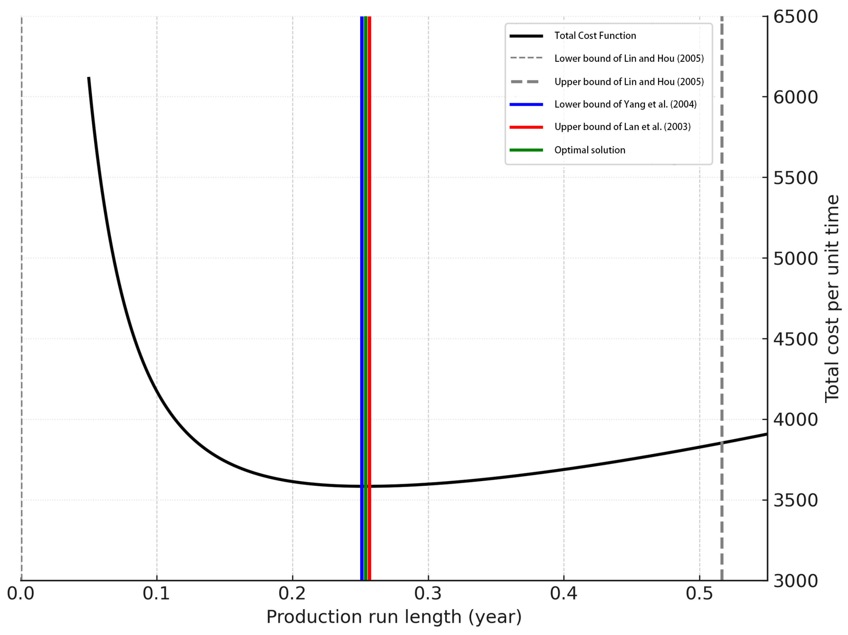
Figure 1 depicts the behavior of the total cost function $\mathrm{T}\mathrm{C}\left(\mathrm{T}\right)$ over a wide range of production run lengths. The curve exhibits a clear unimodal shape, indicating a unique minimum that corresponds to the optimal production cycle length. We also mark the original lower and upper bounds suggested by Lin and Hou [12], alongside our improved bounds based on Chung and Lin [5] and Yang et al. [11]. It is evident that our proposed bounds are much closer to the true minimum, significantly reducing the search interval required for the bisection algorithm.

The black curve in the figure above is the total cost function, which exhibits a convex, bowl-shaped cost with a unique minimum. The green vertical line marks the optimal solution of $\mathrm{T}\mathrm{C}\left(\mathrm{T}\right)$. The blue and red lines on its left and right are the lower bound of [16] and upper bound of [10], respectively—these nearly coincide with the optimum, highlighting the tight bracket achieved by Yang et al. [11] (blue) and Lan et al. [10] (red). The grey-dashed lines at the far left and right represent the lower bound of [12] and upper bound of [12], which are much wider apart, confirming that the newer bounds dramatically improve upon [12]. All lines are clearly distinguishable by color and line style, and the convexity of $\mathrm{T}\mathrm{C}\left(\mathrm{t}\right)$ is visually evident.

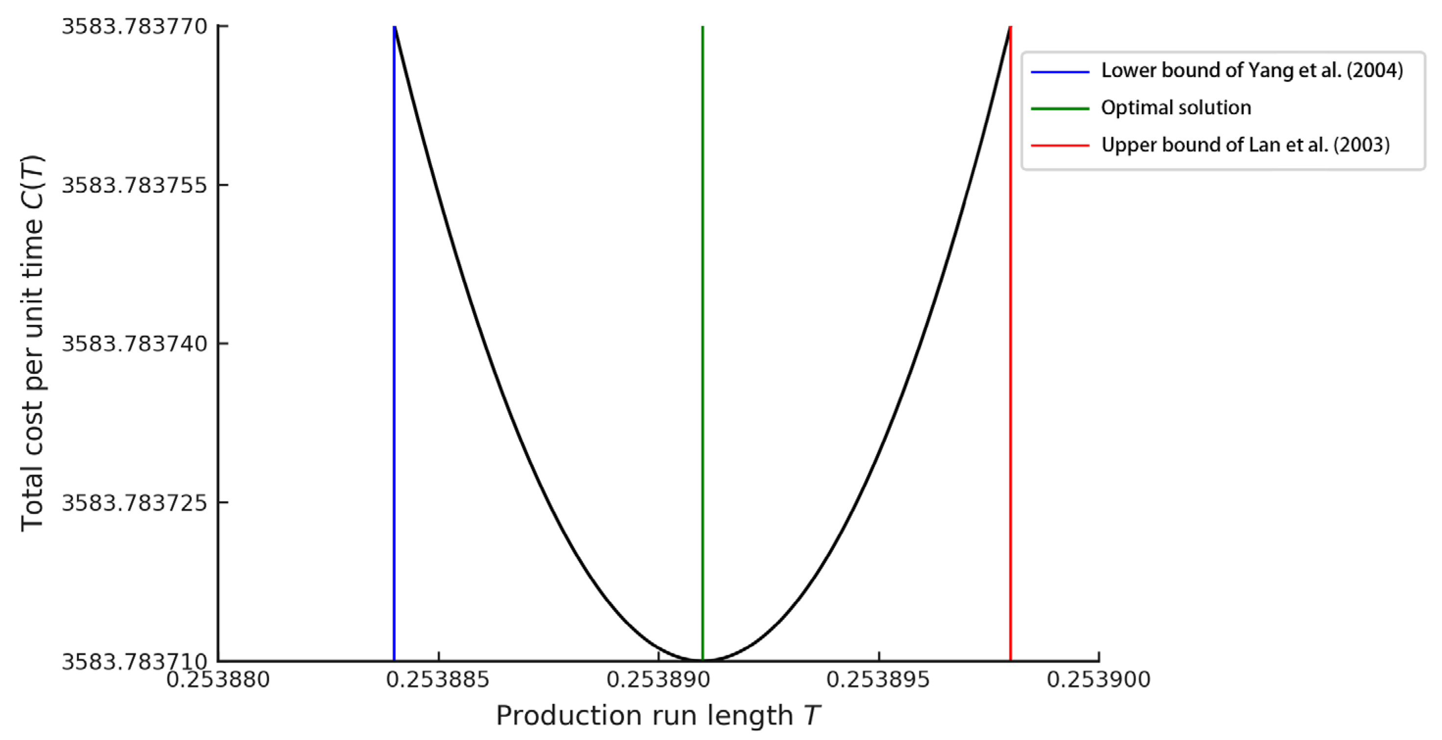
Figure 2 zooms in on the region near the optimal run length to emphasize the precision of the improved bounds. The interval between the new lower and upper bounds is exceedingly narrow, closely bracketing the minimum point of $\mathrm{T}\mathrm{C}\left(\mathrm{t}\right)$. This clearly demonstrates the improved efficiency and accuracy of our approach in locating the optimal solution.

The figure above clearly illustrates how much closer the improved bounds are to the true optimum compared to the initial bounds of [12].

Figure 3 compares the absolute error in approximating the exponential function ${\mathrm{e}}^{-\mathrm{x}}$ using various methods. The upper-bound approximation by Chung and Lin [5] has the highest error across the domain, while the lower-bound method by Yang et al. [11] produces the smallest error. This justifies why the bounds derived from Yang et al. [11] lead to near-optimal solutions with minimal iteration.

These visualizations not only confirm the analytical strength of our improvements, but also enhance the interpretability of the model’s behavior and its sensitivity to exponential function estimation. They further illustrate the practical advantage of applying more accurate approximations in minimizing computational effort and ensuring solution precision.

6. Formulated Approximated Solution

Our previous discussion yields that our lower bound, ${\mathrm{x}}_{\mathrm{L}\mathrm{B}}\left(1\right)$, and upper bound, ${\mathrm{x}}_{\mathrm{U}\mathrm{B}}\left(1\right)$, are very close approximations for the optimal solution. Hence, we will apply Equations (24) and (26) simultaneously to solve ${\mathrm{L}\mathrm{B}}_1\left(\mathrm{x}\right)=0$ and ${\mathrm{U}\mathrm{B}}_1\left(\mathrm{x}\right)=0$ to find a formulated approximation for the optimal solution as follows: We have

$${\mathrm{a}}_1{\mathrm{x}}^4+4{\mathrm{a}}_1{\mathrm{x}}^3+\left(6{\mathrm{a}}_1+{\mathrm{a}}_0-3\mathsf{\beta }\right){\mathrm{x}}^2+4{\mathrm{a}}_0\mathrm{x}+6{\mathrm{a}}_0=0,$$

(49)

and

$$\left(2{\mathrm{a}}_1+\mathsf{\beta }\right){\mathrm{x}}^3+\left(6{\mathrm{a}}_1-3\mathsf{\beta }\right){\mathrm{x}}^2+2{\mathrm{a}}_0\mathrm{x}+6{\mathrm{a}}_0=0,$$

(50)

where

$${\mathrm{a}}_0=-\left(\mathrm{d}\mathrm{k}/\mathrm{p}\right),$$

(51)

and

$${\mathrm{a}}_1=\mathrm{h}\left(\mathrm{p}-\mathrm{d}\right)/2{\mathsf{\lambda }}^2.$$

(52)

We multiply Equation (49) by $\left(2{\mathrm{a}}_1+\mathsf{\beta }\right)$ and then subtract the multiplication of Equation (50) by ${\mathrm{a}}_1\mathrm{x}$ to imply that

$${\mathrm{a}}_1\left(2{\mathrm{a}}_1+7\mathsf{\beta }\right){\mathrm{x}}^3+\left[3\left(4{\mathrm{a}}_1^2-{\mathsf{\beta }}^2\right)+\mathsf{\beta }{\mathrm{a}}_0\right]{\mathrm{x}}^2+2{\mathrm{a}}_0\left({\mathrm{a}}_1+2\mathsf{\beta }\right)\mathrm{x}+6{\mathrm{a}}_0\left(2{\mathrm{a}}_0+\mathsf{\beta }\right)=0,$$

(53)

If we cancel out ${\mathrm{x}}^3$ from the two cubic polynomials in Equations (50) and (53), then a quadratic equation is achieved:

$${\mathrm{b}}_2{\mathrm{x}}^2+{\mathrm{b}}_1\mathrm{x}+{\mathrm{b}}_0=0,$$

(54)

with the coefficients

$${\mathrm{b}}_2=3\left({\mathrm{a}}_1-\mathsf{\beta }\right){\left({2\mathrm{a}}_1-\mathsf{\beta }\right)}^2+\mathsf{\beta }{\mathrm{a}}_0\left(2{\mathrm{a}}_1+\mathsf{\beta }\right),$$

(55)

$${\mathrm{b}}_1=4\mathsf{\beta }{\mathrm{a}}_0\left(\mathsf{\beta }-{\mathrm{a}}_1\right),$$

(56)

and

$${\mathrm{b}}_0=6{\mathrm{a}}_0\left({\mathrm{a}}_1-\mathsf{\beta }\right)\left({2\mathrm{a}}_1-\mathsf{\beta }\right).$$

(57)

If we check the value of

$$\left[\left(-{\mathrm{b}}_1+\sqrt{{\mathrm{b}}_1^2-4{\mathrm{b}}_2{\mathrm{b}}_0}\right)/2{\mathrm{b}}_2\right]/\mathsf{\lambda }=0.253894,$$

(58)

this is very close to the optimal manufacture run length, ${\mathrm{t}}^{\ast }=0.253891$, of Equation (47). Moreover, the total cost evaluated at our formulated approximation of Equation (58) attains the minimum solution as

$$\mathrm{T}\mathrm{C}\left({\mathrm{t}}^{\#}\right)=3583.784.$$

(59)

where

$${\mathrm{t}}^{\#}=0.253894,$$

(60)

is the formulated approximated solution proposed by us in Equation (58).

We recall Çalışkan [43] to claim that closed-form approximations are intuitive and easy to understand and do not require advanced mathematics, making them attractive to practitioners. Furthermore, we note that Çalışkan [44] asserted that numerical studies in the literature show that the approximate solution yields total costs within a tiny fraction, often less than $0.5\%$, of the true optimum. Gijsbrechts et al. [45] analyzed a manufacturer’s inventory policy for when capacity is flexible, and then they proposed a lookahead peak-shaving policy to derive explicit closed-form expressions for time-varying base-stock levels under demand uncertainty. They obtained analytic formulas for the period-dependent reorder points to minimize cost under stochastic demand and capacity conditions. The numerical results from a consumer goods case showed that these formulas reduced inventory and sourcing costs by 7% compared to the firm’s existing policy, demonstrating closed-form analysis in a supply chain inventory context with non-stationary demand. In real-world terms, this means that managers can implement the simplified formula with confidence that any cost increase is negligible, while gaining the benefits of simplicity and speed. These advantages of faster computation, interpretability, and robustness to parameter changes are now clearly expressed by this study.

7. Sensitivity Analysis with Graphical Illustrations

To further investigate the robustness of the proposed model, we conduct a sensitivity analysis on three key parameters: production rate, $\mathrm{p}$, restoration cost, $\mathrm{r}$, and in-control defect rate, ${\mathsf{\theta }}_1$. For each parameter, we observe how variations affect the optimal production run length, ${\mathrm{T}}^{\ast }$, while holding other parameters constant.

Table 3. Sensitivity analysis with respect to the manufacture rate, $\mathrm{p}$.

$\mathbf{p}$	$1300$	$1400$	$1500$	$1600$	$1700$
${\mathrm{t}}^{\ast }$	$0.287516$	$0.269632$	$0.253891$	$0.239924$	$0.227441$
$\mathrm{T}\mathrm{C}\left({\mathrm{t}}^{\ast }\right)$	$3609.629$	$3595.871$	$3583.784$	$3573.077$	$3563.526$
${\mathrm{x}}_{\mathrm{L}\mathrm{B}}\left(1\right)/\mathsf{\lambda }$	$0.287505$	$0.269623$	$0.253884$	$0.239918$	$0.227437$
$\mathrm{T}\mathrm{C}\left({\mathrm{x}}_{\mathrm{L}\mathrm{B}}\left(1\right)/\mathsf{\lambda }\right)$	$3609.629$	$3595.871$	$3583.784$	$3573.077$	$3563.526$
${\mathrm{x}}_{\mathrm{U}\mathrm{B}}\left(1\right)/\mathsf{\lambda }$	$0.287528$	$0.269641$	$0.253898$	$0.239930$	$0.227446$
$\mathrm{T}\mathrm{C}\left({\mathrm{x}}_{\mathrm{U}\mathrm{B}}\left(1\right)/\mathsf{\lambda }\right)$	$3609.629$	$3595.871$	$3583.784$	$3573.077$	$3563.526$
${\mathrm{t}}^{\#}$	$0.287516$	$0.269634$	$0.253894$	$0.239927$	$0.227444$
$\mathrm{T}\mathrm{C}\left({\mathrm{t}}^{\#}\right)$	$3609.629$	$3595.871$	$3583.784$	$3573.077$	$3563.526$

,

Table 4. Sensitivity analysis with respect to the restoration cost, $\mathrm{r}$.

$\mathbf{r}$	$100$	$150$	$200$	$250$	$300$
${\mathrm{t}}^{\ast }$	$0.253811$	$0.253851$	$0.253891$	$0.253931$	$0.253971$
$\mathrm{T}\mathrm{C}\left({\mathrm{t}}^{\ast }\right)$	$3570.783$	$3577.283$	$3583.784$	$3590.284$	$3596.784$
${\mathrm{x}}_{\mathrm{L}\mathrm{B}}\left(1\right)/\mathsf{\lambda }$	$0.253804$	$0.253844$	$0.253884$	$0.253924$	$0.253964$
$\mathrm{T}\mathrm{C}\left({\mathrm{x}}_{\mathrm{L}\mathrm{B}}\left(1\right)/\mathsf{\lambda }\right)$	$3570.783$	$3577.283$	$3583.784$	$3590.284$	$3596.784$
${\mathrm{x}}_{\mathrm{U}\mathrm{B}}\left(1\right)/\mathsf{\lambda }$	$0.253818$	$0.253858$	$0.253898$	$0.253938$	$0.253978$
$\mathrm{T}\mathrm{C}\left({\mathrm{x}}_{\mathrm{U}\mathrm{B}}\left(1\right)/\mathsf{\lambda }\right)$	$3570.783$	$3577.283$	$3583.784$	$3590.284$	$3596.784$
${\mathrm{t}}^{\#}$	$0.253814$	$0.253854$	$0.253894$	$0.253934$	$0.253974$
$\mathrm{T}\mathrm{C}\left({\mathrm{t}}^{\#}\right)$	$3570.783$	$3577.283$	$3583.784$	$3590.284$	$3596.784$

and

Table 5. Sensitivity analysis with respect to the in-control defect rate, ${\mathsf{\theta }}_1$.

${\mathsf{\theta }}_1$	$0.05$	$0.075$	$0.1$	$0.2$	$0.3$
${\mathrm{t}}^{\ast }$	$0.246693$	$0.250215$	$0.253891$	$0.270380$	$0.290516$
$\mathrm{T}\mathrm{C}\left({\mathrm{t}}^{\ast }\right)$	$2364.548$	$2974.275$	$3583.784$	$6019.442$	$8450.710$
${\mathrm{x}}_{\mathrm{L}\mathrm{B}}\left(1\right)/\mathsf{\lambda }$	$0.246687$	$0.250208$	$0.253884$	$0.270372$	$0.290506$
$\mathrm{T}\mathrm{C}\left({\mathrm{x}}_{\mathrm{L}\mathrm{B}}\left(1\right)/\mathsf{\lambda }\right)$	$2364.548$	$2974.275$	$3583.784$	$6019.442$	$8450.710$
${\mathrm{x}}_{\mathrm{U}\mathrm{B}}\left(1\right)/\mathsf{\lambda }$	$0.246700$	$0.250222$	$0.253898$	$0.270389$	$0.290526$
$\mathrm{T}\mathrm{C}\left({\mathrm{x}}_{\mathrm{U}\mathrm{B}}\left(1\right)/\mathsf{\lambda }\right)$	$2364.548$	$2974.275$	$3583.784$	$6019.442$	$8450.710$
${\mathrm{t}}^{\#}$	$0.246695$	$0.250218$	$0.253894$	$0.270385$	$0.290522$
$\mathrm{T}\mathrm{C}\left({\mathrm{t}}^{\#}\right)$	$2364.548$	$2974.275$	$3583.784$	$6019.442$	$8450.710$

present the results of this analysis.

Effect of production rate, $\mathrm{p}$: As shown in Table 3, increasing the production rate from 1300 to 1700 leads to a moderate decrease in ${\mathrm{t}}^{\ast }$ and $\mathrm{T}\mathrm{C}\left({\mathrm{t}}^{\ast }\right)$. On the other hand, for all variations in $\mathrm{p}$, the lower bound, ${\mathrm{x}}_{\mathrm{L}\mathrm{B}}\left(1\right)/\mathsf{\lambda }$, the upper bound, ${\mathrm{x}}_{\mathrm{U}\mathrm{B}}\left(1\right)/\mathsf{\lambda }$, and the closed-form approximated solution, ${\mathrm{t}}^{\#}$, all attain the optimal value. This is because a higher production rate improves inventory turnover, reducing the holding cost per unit time and favoring shorter cycles. However, the effect is relatively mild, indicating that the model is not highly sensitive to moderate changes in $\mathrm{p}$.

Effect of restoration cost, $\mathrm{r}$: Table 4 demonstrates that as the restoration cost increases from 100 to 300, the optimal run length slightly increases. On the other hand, for all variations in $\mathrm{r}$, the lower bound, ${\mathrm{x}}_{\mathrm{L}\mathrm{B}}\left(1\right)/\mathsf{\lambda }$, the upper bound, ${\mathrm{x}}_{\mathrm{U}\mathrm{B}}\left(1\right)/\mathsf{\lambda }$, and the closed-form approximated solution, ${\mathrm{t}}^{\#}$, all attain the optimal value. Higher restoration costs make frequent maintenance less desirable, encouraging longer production runs to spread out the fixed cost of restoration over a longer period.

Effect of in-control defect rate, ${\mathsf{\theta }}_1$: The most significant sensitivity is observed with respect to ${\mathsf{\theta }}_1$, as depicted in Table 5. As the in-control defect rate increases from 0.05 to 0.3, the optimal production cycle length increases noticeably. On the other hand, for all variations in ${\mathsf{\theta }}_1$, the lower bound, ${\mathrm{x}}_{\mathrm{L}\mathrm{B}}\left(1\right)/\mathsf{\lambda }$, the upper bound, ${\mathrm{x}}_{\mathrm{U}\mathrm{B}}\left(1\right)/\mathsf{\lambda }$, and the closed-form approximated solution, ${\mathrm{t}}^{\#}$, all attain the optimal value. A higher defect rate increases the rework cost, making it more economical to extend the production run to limit the accumulation of defective items.

This sensitivity analysis provides practical insights into how different operational conditions influence optimal decision-making. In particular, efforts to maintain a low defect rate can substantially impact production planning, while changes in production rate or maintenance costs have comparatively moderate effects.

Based on the results in Table 3, Table 4 and Table 5, we demonstrate that the lower bound, ${\mathrm{x}}_{\mathrm{L}\mathrm{B}}\left(1\right)/\mathsf{\lambda }$, the upper bound, ${\mathrm{x}}_{\mathrm{U}\mathrm{B}}\left(1\right)/\mathsf{\lambda }$, and the closed-form approximated solution, ${\mathrm{t}}^{\#}$, all attain the optimal value, such that there are nineteen examples to support us to claim the robustness of our proposed lower bound, upper bound, and closed-form approximated solution.

8. Contributions and Limitations

In this study, we developed refined analytical bounds for the EMQ model and demonstrated their effectiveness through theoretical analysis and a numerical example. The results show that our improved lower and upper bounds dramatically reduce the search interval for the bisection algorithm, enabling a much faster convergence to the optimal solution. In fact, in the example we examined, the initial interval containing the optimal solution was reduced to less than 1% of its original length when using our bounds, as compared to the original approach by Lin and Hou [12]. Consequently, the production run length identified by our method yields an average total cost that is virtually identical to the true minimum. These findings confirm that the proposed bounding technique significantly enhances the precision of the EMQ model’s solution without adding computational complexity, which is a valuable outcome for both researchers and practitioners dealing with similar inventory models. Despite the improvements achieved, there are certain limitations to this work. First, our model assumes a specific structure for the production process (e.g., a single product, a two-state in-control/out-of-control process with exponential failure distribution) and relies on known parameter values for costs and defect rates. In practice, these parameters may be uncertain or time-varying, and the performance of the proposed method under such uncertainty would require further investigation. Second, the analytical bounds we derived are based on conditions that ensure that the cost function behaves in an unimodal manner. If the underlying assumptions (such as the restrictions on defect probabilities or cost relationships) are violated, the effectiveness of the bounds may be diminished. Additionally, our approach is focused on improving solution accuracy rather than addressing broader extensions of the EMQ problem. Future research could explore combining our bounding technique with other extensions of the EMQ model—such as multi-stage production systems, learning effects, or stochastic demand and maintenance schedules—to assess its applicability in more complex settings. Finally, while we provided one illustrative example and a sensitivity analysis, more extensive computational experiments could be conducted to further validate the robustness of the proposed method across different scenarios.

9. Conclusions

This paper re-examines the economic manufacturing quantity model under imperfect production conditions and introduces refined bounds for the bisection algorithm. By tightening the lower and upper bounds of the cost function’s root-finding interval, our approach dramatically improves the precision of the approximated optimal solution. The numerical results indicate that the initial search interval can be shrunk to less than 1%, and the proposed approximated run length yields a total cost essentially equal to the true minimum cost. These improvements not only validate the effectiveness of our method, but also provide a more efficient way to solve such inventory models. Overall, the enhanced bounds and the formulated approximate solution developed in this work contribute to the literature by resolving an open issue in the EMQ model and offering a practical tool for inventory optimization. We hope that the ideas presented here will stimulate further research into integrating analytical bounding techniques with other extensions of production inventory models and inspire the application of this approach to broader scenarios in manufacturing systems.