The Stochastic Evolution of Financial Asset Prices

Abstract

This paper examines the relationship between dependence and independence alternatives in general stochastic processes and explores the duality between the true (yet unknown) stochastic process and the functional representation that fits the observed data. We demonstrate that the solution depends on its historic realizations, challenging existing theoretical frameworks that assume independence between the solution and the history of the true process. Under orthogonality conditions, we investigate parameter spaces within data-generating processes and establish conditions under which data exhibit mean-reverting, random, cyclical, history-dependent, or explosive behaviors. We validate our theoretical framework through empirical analysis of an extensive dataset comprising daily prices from the S&P500, 10-year US Treasury bonds, the EUR/USD exchange rate, Brent oil, and Bitcoin from 1 January 2002 to 1 February 2024. Our out-of-sample predictions, covering the period from 17 February 2019 to 1 February 2024, demonstrate the model’s exceptional forecasting capability, yielding correct predictions with between 73% and 92% accuracy, significantly outperforming naïve and moving average models, which only achieved 47% to 54% accuracy.

1. Introduction

All stochastic sequences and their solutions share the same topological endowments or obey different laws. Determining when an unknown function of a sequence has the same topology as the sequence itself in a truly unbiased manner could be a natural way to test whether asymptotic behaviors can ensure convergence. In such a case, the model matches the observed data. Chichilnisky [1] used weighted Hilbert spaces to identify the convergence of the Fourier coefficients of the unknown function that solves the stochastic sequence for all domains in bounded and unbounded spaces. A Hilbert space is complete and always reflexive. Therefore, solutions to stochastic partial differential equations are always endowed with the inner product that allows the closeness of the known and unknown sequences to be measured and to establish duality in the sense of being reflexive. In an unknown solution in a Hilbert space, the sequence $\mathcal{H}\rho$ would always be isomorphic to a function of $\mathcal{H}S$ that is jointly defined in a uniformly convex space. An observer testing the existence of duality will be biased when measured on the real line $L^2\left(R\right)$. Bergstrom [2] remarks that for a Hilbert space where continuous functions have bounded variation, the square integrable unknown function $\mathcal{H}S:K\mapsto \mathcal{R}$ requires $\underset{K\to \infty }{S\left(K\right)}=0$, representing a very strong restriction as it excludes important functions such as the constant, increasing, and cyclical types (see Chichilnisky [1]).

The Banach space $\mathcal{B}$ is a complete normed space $L^p$ of some dimension p, and it exists between the Hilbert space and a space M which is endowed with a metric and not a norm. In particular, if $\mathcal{L}=\left\{L^1,L^2,\dots ,L^p,\dots ,L^M,\dots ,L^{\infty }\right\}$ with any choice of p is within $2\le p\le M\le \infty$, then it is a Banach space. In addition, the vector probability space, defined by the triplet $\mathcal{L}\left(X,\Omega ,\theta \right)$ is a $\sigma$-finite measure, where X is the particular space, $\mathcal{F}$ represents the filtered measurable sets, and $\theta$ is the measure. Then, more formally, a Banach space is defined as $\mathcal{L}\left(X,\Omega ,\theta \right):=\left(f:X\to C\right)$, with f being $\Omega$ measurable. The direct implication is that ${\int }_X{\left|f\left(x\right)\right|}^{p}d\theta \left(x\right)<\infty$. Completeness means that any Cauchy, C, sequence with respect to the norm is convergent at the point that is in the space. The Banach norm $L^p$ of the function f is given by

$${∥f∥}_p={\left({\int }_X{\left|f\left(x\right)\right|}^{p}d\theta \left(x\right)\right)}^{1/p}$$

(1)

Geometrical considerations for normed spaces are dictated by the value of p. For instance, when $p=1$, we have the space $L^1$ that includes all integrable functions f on X, and the ${∥·∥}_{L^1}$ satisfies the triangle inequality. When $p=2$, $L^2$ is a Hilbert space and ${∥·∥}_{L^2}$.

In general, only square integrable processes that are integrable functions are measurable and include all common functions such as “sup”, “inf”, and “lim”, are unique in being compatible with the desirable inner product property of the Hilbert space, and this guarantees reflexivity. Tsirelson [3] showed an example in which the square integrable sequences are not always isomorphic to a uniformly convex space and they do not obey the same topological laws, while they have no inner product properties. The contribution of this paper is, therefore, to amplify the Hilbert space, with Banach $L^p$ satisfying $L^1<L^2<L^p<\infty$ for any p in $2\le p\dots \le \infty$. The purpose is, then, to extend the limits of measurement and identify the conditions for the duality of the unknown solution and its history via the observed stochastic process. For this, we assume that all functional forms will be measured in a Banach complete normal space, and this is where the $h=\left(H_0,H_1\right)$ will be tested with some probability. We discuss the conditions under which it is isomorphic to a convex reflexive Banach dual space when the observed sequence inherits norms and an inner product. Yano K. [4] demonstrate that the unknown solution space $S_k$ does not depend on the known sequence metric ${\xi }_j$, and this invalidates the use of any functional model for explaining and predicting an unknown related process under orthogonality assumption in random processes. In general, duality and association cannot exist if the unobserved solution is not linked to the observed data. History plays no role in the formation of the new state, and generally speaking, $S_k=\left({\prod }_{-\infty }^k{\xi }_j\right)V$, with V being some other independent sequence. Under this scenario, reversibility is impossible as there is an infinite number of starting points to map going backwards, rendering the course of the observed sequence unpredictable.

In this paper, we discuss the dependence and independence alternatives for a general stochastic solution process, and when the stochastic process takes values from Banach space, we examine under which conditions it can be reflexive. In particular, we examine whether the stochastic process depends on its known history. We argue that multidimensional integration has duality in a reflexive Banach space if the solution obeys the functional central limit theorem and its error is between the limits of dilation and erosion. Hence, there is isomorphism for closed and semi-open intervals and the desired inner product to define the orthogonality conditions. The evolution process depends on its history in three-quarters of all existing probability measures, and this necessarily implies that the integrable curves are quasi-periodic depending only on initial conditions that can be found in history, or indeed at the beginning of the cosmos. One possible scenario is, as Yano K. [4] and Tsirelson [3] suggested, that no model exists and reversibility is unattainable as it would map to infinite possible initial points. We offer a framework to evaluate these scenarios under different novel models that capture the general family of possible null hypotheses formulations. They can capture all possibilities of dependence and independence in both Banach and reflexive Banach spaces.

Still following their assumptions and adopting the compact G group and requiring duality in reflexive Banach space, we prove their dependence. We derive the orthogonality conditions and show that the unknown unique stochastic solution would depend on the observable history of the sequence, as in $S_m={\prod }_{-\infty }^m{\rho }_j{S}_{m-1}$. The evolution process would depend on its history in three-quarters of all existing scenarios. When variation is outside the limits of dilation and erosion, the space will be composed of countably additive and possibly finitely additive measures with no functional representation in $\mathcal{B}$. Convergence will also fail in this scenario.

This paper contributes to several strands of the literature at the intersection of stochastic process theory, functional analysis in infinite-dimensional spaces, and empirical time series modeling under structural complexity. Below, we situate our work within four key domains: (1) duality and functional representation in Banach and Hilbert spaces; (2) dependence, orthogonality, and predictability in stochastic systems; (3) modeling nonstationary financial time series with structural breaks; and (4) empirical applications and computational limits in high-volatility environments.

The representation of stochastic processes in infinite-dimensional spaces has long been shaped by the use of Hilbert spaces due to their inner product structure and reflexivity [1,2]. However, this approach imposes strong topological restrictions—such as the exclusion of constant or monotonic functions—and often fails to accommodate non-smooth or heavy-tailed processes. Demonstrated by [3] square-integrable sequences do not always exhibit topological equivalence with uniformly convex function spaces, posing limitations for models based solely on $L^2$ spaces.

Recent advancements extend duality and learning representations to more general settings. For instance, [5] explored duality principles in reproducing kernel Banach spaces (RKBS), offering a functional framework beyond Hilbert geometries. Further [6] formalized the duality of spaces of càdlàg (right-continuous with left limits) processes, establishing foundational conditions for reflexivity in stochastic filtrations. We extend these approaches by situating the stochastic solution within a reflexive Banach space $L^p$ for $p>2$, allowing for a more general functional topology. This enables the definition of duality between observed and unobserved sequences, even in the absence of inner products, and provides a novel isomorphism mapping via convolutional sequences in ${\rho }_k$. Unlike prior models, our construction supports a broader family of functional forms—including explosive, cyclic, and path-dependent dynamics—within a coherent probabilistic geometry.

In their work [4] present a formal case in which the evolution process $S_k$ is orthogonal to its observed history, invalidating the use of predictive functional forms. Under their framework, the absence of duality renders the process fundamentally irreversible and unpredictable. Davidson, in [7,8] explore related concerns in the context of I(0) processes and the functional central limit theorem. More recently, orthogonality structures have gained attention in spectral analysis and stochastic modeling. Generalized polynomial chaos expansions benefit from orthogonality in solving stochastic PDEs, though this work remains largely applied to physical systems [9]. Our work complements these efforts by deriving a precise orthogonality condition,

$$E[g(k-1)·{ϵ}_k\left(p\right)]=0\iff w_k=1,$$

which we use to classify regimes as martingale, trend-following, mean-reverting, or explosive.

Here, we reintroduce history as a structural feature of stochastic evolution, showing that in three-quarters of all probabilistic configurations, the solution $S_k$ is dependent on its past. The moment-generating function ${\varphi }_k\left(p\right)$ and its innovation ${ϵ}_k\left(p\right)$ serve as instruments for detecting and classifying the nature of dependence. This builds a dynamic model of predictability that is entirely endogenous to the data-generating process.

Traditional time series models—such as ARMA, GARCH, and their extensions—typically assume stationarity or impose transformations (e.g., differencing) to induce it [10]. However, real-world financial series are nonstationary, exhibit volatility clustering, and often undergo abrupt structural changes. Structural break detection is typically addressed via exogenous methods, such as in [11], though these are not integrated into the modeling process.

The recent work by [12] checked for multiple breaks without imposing prior distributional knowledge by proposing a nonparametric change-point detection approach to estimate the number of change points and their locations along the temporal axis.

The AREM model used in this study integrates break detection directly into its stochastic foundation via the behavior of the $w_k$ statistic and the divergence of ${\varphi }_k\left(p\right)$. Rather than treating structural breaks as exogenous events, the model flags them as a breakdown of orthogonality, thereby internalizing regime shifts. Moreover, the recursive form $S_k={\prod }_{j=-\infty }^k{\rho }_j·S_{k-1}$ provides a continuous, historical basis for modeling long memory and path dependence, rather than differencing away valuable information.

On the empirical front, studies have emphasized the need for forecasting models to perform under heavy tails and computational constraints. In particular, ref. [13] introduced fractional Brownian motion to describe persistent memory, while [14] proposed models that adapt to macro shifts via spline-GARCH processes. However, these models often require specific distributional assumptions or lack general theoretical foundations.

Recent comparative studies between econometric modeling and machine learning highlight the strengths and limitations of both approaches, particularly under complex dynamic conditions. For instance, ref. [15] analyzed the forecasting of COVID-19’s spread using classical mathematical models versus machine learning techniques, showing that while machine learning often excels in short-term pattern recognition, structural mathematical models offer greater transparency, interpretability, and robustness—especially in the presence of regime shifts and noisy inputs. This trade-off is also relevant in financial time series forecasting, where structural stability and duality-based interpretability are critical. Furthermore, the increasing use of predictive models in financial infrastructure raises significant cybersecurity concerns, as model transparency affects vulnerability to adversarial attacks. Our model, based on recursive structural properties and orthogonality principles, is inherently interpretable, and thus potentially more resilient to such threats. This reinforces the value of functional–theoretic approaches alongside, and often in contrast to, black-box machine learning models.

The empirical application of AREM to diverse assets including Bitcoin, the S&P 500, and US Treasury bonds demonstrates forecasting accuracy between 73% and 93%. This robustness is achieved despite volatility, structural breaks, and nonstationarity, without relying on transformation or external break detection. Further, we formalize the model’s limits of computation via the divergence of dilation/erosion boundaries and propose extensions to switch estimation regimes when orthogonality fails. This positions AREM as both a theoretically grounded and practically adaptive forecasting tool.

In contrast to prior work that either imposes restrictive topologies (Hilbert spaces), neglects historical dependence (orthogonality assumptions), or addresses regime changes exogenously, this paper introduces a unified framework for stochastic modeling based on Banach space duality. Our contributions span foundational theory, the identification of dependence regimes, and high-performing empirical forecasting, all within a mathematically rigorous and computationally tractable setting.

The existing literature provides a rich and multi-dimensional foundation for understanding duality, orthogonality, and predictability in stochastic systems, particularly in the presence of nonstationarity, structural breaks, and nonlinear dependencies. While these works vary in domain and methodology from functional analysis to machine learning, they collectively emphasize the limitations of assuming independence between a stochastic process and its history, as well as the potential gains from exploiting the hidden structure through richer model representations. Others [16] extends Tsirelson’s counterexample by constructing stochastic difference equations on general topological groups. His work demonstrates the existence of stochastic processes that are fundamentally irreversible and independent of their historical trajectories, offering an abstract mathematical example of how history may fail to determine the future. This view aligns with the theoretical boundary proposed by [4], where orthogonality between a process and its past leads to unpredictability and non-reversibility. However, our model challenges this boundary by establishing conditions in reflexive Banach spaces under which dependence on history is restored for most probabilistic configurations. Research by [17] produce a framework for duality in interacting stochastic systems using orthogonal polynomial expansions. By constructing dual processes, they demonstrate that complex dynamics can often be re-expressed in terms of more tractable counterparts. Similarly, we use orthogonality conditions and moment-generating functions to classify regimes of dependence, trend-following, and explosiveness within a unified data-generating process. Moreover [18] offer an important shift by conducting functional time series analysis in Banach rather than Hilbert spaces. By abandoning the inner product structure, they develop new prediction methods under the supremum norm. Our model similarly adopts Banach topology, particularly for $p>2$, to embed historical dependence in spaces that better reflect the irregularity and volatility of real-world time series. This allows us to characterize duality and convergence in a setting where smoothness and completeness are not guaranteed by construction.

Recent econometric contributions, such as those by [19,20,21], develop tools to detect structural breaks in regression relationships. These tests highlight the fragile nature of forecast models when exposed to regime shifts. In contrast to treating such breaks exogenously, our model internalizes them through shifts in the $w_k$ statistic and the divergence of moment-generating functions. This endogeneity allows the AREM model to dynamically adapt to changing regimes, identifying pockets of predictability and divergence from orthogonality without manual intervention.

The question of whether predictability itself is episodic rather than constant is central to [22]. These authors introduce rolling and recursive tests to identify such episodes, aligning with our notion that the orthogonality condition may hold only intermittently. We formalize this through a model where the evolution process $S_k$ depends on its historical path in three-quarters of the probability space.

Modern forecasting research has expanded the toolkit beyond linear models. Studies such as those by [23,24,25] explore the use of ensemble methods and hybrid models to improve forecast accuracy in the presence of complex, nonlinear dependencies. Our AREM model builds on this insight by incorporating ensemble structures that blend multiple predictors—some driven by theory, others by empirical fitting—under a common orthogonality framework.

Neural forecasting models, as reviewed by [26], further extend this logic by allowing for the automatic learning of long memory, seasonality, and regime shifts. These architectures, particularly attention-based and sequence-to-sequence models, can be interpreted as data-driven analogues to our theoretically derived dual systems, while our model is not neural in implementation, it shares the architectural goal of tracking temporal dependencies through recursive structures and regime-adaptive filtering.

Other contributions, such as those by [27,28], stress the need for forecasting models that remain robust in the face of volatility clustering and regime instability. Our approach advances this line of research by constructing a theoretical space within the reflexive Banach framework, where such volatility is not just accommodated, but is endogenous to the model’s structural form.

The next section introduces dependency and a stochastic process that captures the past, present, and future. In Section 3, we provide empirical estimations and results. Section 4 presents the conclusions of this paper.

2. History Matters

We examine the limits of computation that are conditional on the properties endowed to generating the estimated processes. Let us consider the behavior of an unknown process, S, which presents a known correlation function, $\rho$, under a complete normed (Banach) space, so that the comparison of S and $\rho$ can be performed through their respective norms, $\left|\right|·\left|\right|$, alone. Note that two norms are equivalent if $\left|\right|S\left|\right|\le \theta \left|\right|\rho \left|\right|$, for all $\theta =\{S,\rho \}$. Let us further assume that the relation between the two random processes, ${\left(S_k\right)}_{k\le 0}$ and ${\left({\rho }_k\right)}_{k\le 0}$, is characterized by

$$\begin{array}{cc}\hfill S_k=& e^{2i\pi u_k}={\rho }_k{S}_{k-1}\hfill \end{array}$$

(2)

$$\begin{array}{cc}\hfill {\rho }_k=& e^{2i\pi {\theta }_k}\hfill \end{array}$$

(3)

such that k varies in $-\mathbb{N}$, $u_k$ is a standard Gaussian which shares a portion of information, ${\widehat{\theta }}_k$, with ${\theta }_k\in \left[0,1\right)$,

$$\begin{array}{c}\hfill {\theta }_k={\theta }_k^{\perp }+{\widehat{\theta }}_k\end{array}$$

(4)

and ${\left({\rho }_k\right)}_{k\le 0}$ behaves as a Markov chain, with transition probabilities given by

$$\mathbb{P}\left(S_k\in A|{\mathbb{F}}_{k-1}^S\right)=g_k\left(A{\rho }_{k-1}^{-1}\left(\omega \right)\right),A\in \mathbb{B}\left(\mathbb{G}\right)$$

(5)

so that the law ${\rho }_k$ is a given probability ${\left(g_k\right)}_{k\le 0}$ on $\mathbb{G}$, and Equation (1) can be interpreted as a re-statement of the Tsirelson equation, where dependence is introduced by means of ${\rho }_k$. As we could always write $S_k={\displaystyle \frac{m_k}{m_{k-1}}}$, this specification implies that $S_k$ converges to a nonstationary unit root process.

$$\begin{array}{c}\hfill {\rho }_k={\displaystyle \frac{S_k{S}_{k-2}}{S_{k-1}^2}}{\rho }_{k-1}\end{array}$$

(6)

We want to describe the group of laws of the probability ${\mathcal{P}}_g$ of all solutions of Equation (5), and also its behavior at the extreme boundaries $ex\left({\mathcal{P}}_g\right)$. The strong solutions set is ${\mathcal{L}}_g$ under the measure $\mathbb{P}$ as $P,F_k^S\subset F_k^{\rho }$. From Equation (1), we write the identity

$${\rho }_k=S_k{S}_{k-1}^{-1}$$

(7)

We can state that the measure $\mathbb{P}\in {\mathcal{L}}_g$ if $F_k^S=F_k^{\rho }$, meaning that the changes in ${\varphi }_k\left(·\right)$ cannot be explained by the previous period’s relevant information when only the evolution of the $S_k$ process is taken into account. We further assume that ${\widehat{\theta }}_k=u_k+\Delta u_k$ and define ${\varphi }_k\left(·\right)$ the moment-generating function for ${\rho }_k\in \left(-\infty ,+\infty \right)$:

$$\begin{array}{c}\hfill {\varphi }_k\left(p\right):=E\left[e^{\left(2i\pi p{\theta }_k\right)}\right]=E\left[e^{\left(2i\pi p\left({\theta }_{k-1}+\Delta u_k-\Delta u_{k-1}\right)\right)}\right]\end{array}$$

(8)

so that the relation between two consecutive moment-generating functions can be written as

$$\begin{array}{c}\hfill {\varphi }_k\left(p\right)E\left[e^{\left(2i\pi p{\widehat{\theta }}_{k-1}\right)}\right]={\varphi }_{k-1}\left(p\right)E\left[e^{\left(2i\pi p\left({\widehat{\theta }}_{k-1}+\Delta u_k-\Delta u_{k-1}\right)\right)}\right]\end{array}$$

(9)

or, equivalently,

$$\begin{array}{c}\hfill \mathbb{E}\left(g\left(k-1\right)·\left({\varphi }_k\left(p\right)-w_k{\varphi }_{k-1}\left(p\right)\right)\right)=0\end{array}$$

(10)

where $g(k-1)=e^{2i\pi p{\widehat{\theta }}_{k-1}}$ and $w_k={\displaystyle \frac{S_k{S}_{k-2}}{S_{k-1}^2}}$. If we then define the innovation, $ϵ$, as the change between two consecutive moment-generating functions, ${ϵ}_k\left(p\right)={\varphi }_k\left(p\right)-{\varphi }_{k-1}\left(p\right)$, Equation (9) can be restated as

$$\begin{array}{c}\hfill \mathbb{E}\left[g\left(k-1\right)·{ϵ}_k\left(p\right)\right]=\mathbb{E}\left[-\left(1-w_k\right)g\left(k-1\right)\right]·{\varphi }_{k-1}\left(p\right)\end{array}$$

When the process S behaves as a martingale for a period of time, the correlation function will stay unchanged, ${\rho }_k={\rho }_{k-1}$, $w_k=1$ and $\mathbb{E}\left[g\left(k-1\right)·{ϵ}_k\left(p\right)\right]=0$; otherwise, the moment-generating function, ${\varphi }_k\left(p\right)$, must satisfy the general orthogonality conditions over the open interval $\left[0,1\right)$.

Thus, we require the following on the left side:

$$\begin{array}{c}\hfill \mathbb{E}\left[e^{2i\pi p{\widehat{\theta }}_{k-1}}\left({\varphi }_k\left(p\right)-{\varphi }_{k-1}\left(p\right)e^{2i\pi p\left(\Delta u_k-\Delta u_{k-1}\right)}\right)\right]=0\end{array}$$

(11)

and the right side of the interval has to be

$$\begin{array}{c}\hfill \mathbb{E}[\left({\displaystyle \frac{{\varphi }_k\left(p\right)e^{2i\pi p{\widehat{\theta }}_{k-1}}}{{\varphi }_{k-1}\left(p\right)e^{2i\pi p(\Delta u_k-\Delta u_{k-1})})}}\right]\ne 1\end{array}$$

(12)

The following ratio of probabilities is a square integrable process in $L_2\left[a,b\right]$ describing the behavior of the unknown function. To be convergent in the open interval, the relative likelihoods have to be a different value than one. Therefore, we consider

$$\begin{array}{c}\hfill \mathcal{H}E\left[{\displaystyle \frac{{\varphi }_k\left(p\right)·g\left(k-1\right)}{{\varphi }_{k-1}\left(p\right)·g\left(k-1\right)w_k}}\right]=\mathcal{H}E\left[exp\left(2i\pi p{\displaystyle \frac{{\rho }_k}{{\rho }_{k-1}}}\right)\right]\end{array}$$

$$\begin{array}{c}\hfill =exp\left(2i\pi p{\displaystyle \frac{\parallel {\rho }_k{\parallel }_1}{\parallel {\rho }_k{\parallel }_2}}\right)\end{array}$$

(13)

Strong solutions exist if and only if the infinite product is convergent to the Fisher information ratio in the Fourier space, where the periodic functions reside:

$$\underset{k\to -\infty }{lim}exp\left(2i\pi p{\displaystyle \frac{\parallel {\rho }_k{\parallel }_1}{\parallel {\rho }_k{\parallel }_2}}\right)\mapsto e^{2·\mathcal{H}i\pi {\displaystyle \frac{{\mu }_k^B}{{\sigma }_k}}}$$

(14)

with ${\mu }_k={∥{\rho }_k∥}_1={\int }_U\left|S\left(u\right)\right|d\theta \left(u\right)$ and ${\sigma }_k={∥{\rho }_k∥}_2={\left({\int }_U{\left|S\left(u\right)\right|}^{2}d\theta \left(u\right)\right)}^{1/2}$, and then it follows that

$$\mathbb{P}\left({\displaystyle \frac{S_k}{S_{k-1}}}\in A|F_u^{k-1}\right)=e^{2·i·\pi {\displaystyle \frac{{\mu }_k^B}{{\sigma }_k}}}A\left(\omega \right),A\in \mathbb{B}\left(G\right)$$

(15)

Chichilnisky also dealt with open Hilbert spaces, placing conditions on the asymptotic behavior of the unknown function, and in particular the Fourier estimator convergence at infinity. All the fixed points given by this solution for the stochastic process $S_k$ are of the type

$$S_k=\prod _{-\infty }^k{\rho }_k·S_{k-1}$$

(16)

This is an example of the metrics of $G\subset B^{*}$ space, describing the convolution of long and short memory of the processes. In fact, it is an adjusted Tsirelson stochastic process (see [3]). We write the spread difference as a general process that combines in one functional form the Brownian and OU processes conditioned on the speed of reversion, $\lambda$, and the intensity of those changes, $\alpha$. It mixes the two stochastic distributions.

$$\begin{array}{c}\hfill d{S}_t=\lambda \left[\left({\displaystyle \frac{{\mu }_t-r}{\lambda {\sigma }_{S,t}}}-{\displaystyle \frac{\left(1/t+\lambda +\alpha \right)}{\lambda }}{S}_t-S_k\right)\right]dt+{\sigma }_{t}d{W}_t\end{array}$$

(17)

where $S_k={\prod }_{-\infty }^k{\rho }_k·S_{k-1}$, with $t>k$.

A martingale process is one where the expected value of $S_t$ at the next step equals its current value, considering all past information. For $S_t$ to be a martingale, the drift term would need to be zero, or the expectation of future changes would need to balance out to zero. This is unlikely given the structure of the drift term unless very specific conditions are met regarding ${\mu }_t$, r, ${\sigma }_{S,t}$, and the historical term $S_k$.

Explosive behavior refers to $S_t$ moving away from any bound or mean at an accelerating rate. This could occur if $S_k$ dominates and grows without bounds, or the drift term consistently adds to $S_t$ without any counteracting mean-reversion force, and the influence of $S_k$ or the drift term grows over time. ${\displaystyle \frac{\left(1/t+\lambda +\alpha \right)}{\lambda }}{S}_t$: The $1/t$ component decreases over time, modifying the impact of $S_t$ on its drift; while $1/t$ itself is not cyclical, it influences how the strength of the mean-reversion or trend component decays over time. $S_k$, the historical term, integrates past values of S and ${\rho }_k$. If ${\rho }_k$ (and thus $S_k$) incorporates cyclical behaviors, it could induce similar patterns in $S_t$, depending on how significantly $S_k$ influences the overall drift.

First, we simplify the SDE for $S_t$ by expanding the first term inside the square brackets and using the product rule for $S_k$:

$$\begin{array}{cc}\hfill & d{S}_t=\lambda \left[\left({\displaystyle \frac{{\mu }_t-r}{\lambda {\sigma }_{S,t}}}\right)-{\displaystyle \frac{1}{\lambda }}\left({\displaystyle \frac{1}{t}}+\lambda +\alpha \right)S_t+{\displaystyle \frac{1}{\lambda }}\prod _{-\infty }^k{\rho }_k·S_{k-1}\right]dt+{\sigma }_{t}d{W}_t\hfill \\ \hfill & =\lambda \left[{\displaystyle \frac{{\mu }_t-r}{\lambda {\sigma }_{S,t}}}-{\displaystyle \frac{1}{\lambda }}\left({\displaystyle \frac{1}{t}}+\lambda +\alpha \right)S_t\right]dt+{\displaystyle \frac{1}{\lambda }}\prod _{-\infty }^k{\rho }_k·S_{k-1}·\lambda dt+{\sigma }_{t}d{W}_t\hfill \\ \hfill & ={\displaystyle \frac{{\mu }_t-r}{{\sigma }_{S,t}}}dt-{\displaystyle \frac{1}{\lambda }}\left({\displaystyle \frac{1}{t}}+\lambda +\alpha \right){\sigma }_{S,t}{S}_{t}dt+{\displaystyle \frac{1}{\lambda }}\prod _{-\infty }^k{\rho }_k·S_{k-1}·\lambda dt+{\sigma }_{t}d{W}_t\hfill \\ \hfill & ={\displaystyle \frac{{\mu }_t-r}{{\sigma }_{S,t}}}dt-{\displaystyle \frac{\left(\frac{1}{t}+\lambda +\alpha \right)}{\lambda }}{\sigma }_{S,t}{S}_{t}dt+{\displaystyle \frac{1}{\lambda }}\prod _{-\infty }^k{\rho }_k·S_{k-1}·\lambda dt+{\sigma }_{t}d{W}_t\hfill \\ \hfill & ={\displaystyle \frac{{\mu }_t-r}{{\sigma }_{S,t}}}dt-\left({\displaystyle \frac{1}{t\lambda }}+{\displaystyle \frac{1}{{\lambda }^2}}+{\displaystyle \frac{\alpha }{\lambda }}\right){\sigma }_{S,t}{S}_{t}dt+{\displaystyle \frac{1}{\lambda }}\prod _{-\infty }^k{\rho }_k·S_{k-1}·\lambda dt+{\sigma }_{t}d{W}_t\hfill \end{array}$$

Next, we apply Ito’s Lemma to the function $f(S_t,t)=ln\left(S_t\right)$. Applying Ito’s Lemma to the function $f(S_t,t)=ln\left(S_t\right)$, we obtain

$$\begin{array}{cc}\hfill & df(S_t,t)=f_{t}dt+f_{S}d{S}_t+{\displaystyle \frac{1}{2}}{f}_{SS}{\left(d{S}_t\right)}^2\hfill \\ \hfill & ={\displaystyle \frac{1}{S_t}}d{S}_t-{\displaystyle \frac{1}{2}}{\displaystyle \frac{1}{S_t^2}}{\left(d{S}_t\right)}^2\hfill \end{array}$$

using the fact that $f_t=0$, $f_S={\displaystyle \frac{1}{S_t}}$, and $f_{SS}=-{\displaystyle \frac{1}{S_t^2}}$.

Substituting the expression for $d{S}_t$ in terms of $S_t$, ${\mu }_t$, ${\sigma }_{S,t}$, and $S_k$, we obtain

$$\begin{array}{cc}\hfill & df(S_t,t)={\displaystyle \frac{\lambda }{S_t}}\left({\displaystyle \frac{{\mu }_t-r}{\lambda {\sigma }_{S,t}}}-{\displaystyle \frac{1}{\lambda }}(1/t+\lambda +\alpha )S_t-S_k\right)dt+{\displaystyle \frac{{\sigma }_t}{S_t}}d{W}_t-{\displaystyle \frac{1}{2}}{\displaystyle \frac{1}{S_t^2}}{\sigma }_t^{2}dt\hfill \\ \hfill & =\left[{\displaystyle \frac{{\mu }_t-r}{{\sigma }_{S,t}}}-\left({\displaystyle \frac{1}{t}}+\lambda +\alpha \right)S_t-{\displaystyle \frac{{\sigma }_t^2}{2S_t^2}}+{\displaystyle \frac{\lambda }{S_t}}{S}_k\right]dt+{\displaystyle \frac{{\sigma }_t}{S_t}}d{W}_t\hfill \end{array}$$

using the fact that ${\displaystyle \frac{\lambda }{{\sigma }_{S,t}}}={\displaystyle \frac{1}{{\sigma }_{I,t}}}$ and $S_k$ is a function of past realizations of $S_t$, and is therefore deterministic.

We can integrate both sides of this equation from 0 to t to obtain

$$\begin{array}{cc}\hfill & ln\left(S_t\right)-ln\left(S_0\right)={\int }_0^t\left({\displaystyle \frac{{\mu }_u-r}{\lambda {\sigma }_{S,u}}}-{\displaystyle \frac{(1/u+\lambda +\alpha )}{\lambda }}{S}_u-S_k-{\displaystyle \frac{1}{2}}{\left[{\displaystyle \frac{1}{S_u}}{\sigma }_u\right]}^2\right)du+{\int }_0^t{\displaystyle \frac{1}{S_u}}{\sigma }_{u}d{W}_u\hfill \\ \hfill & ln\left(S_t\right)=ln\left(S_0\right)+{\int }_0^t\left({\displaystyle \frac{{\mu }_u-r}{\lambda {\sigma }_{S,u}}}-{\displaystyle \frac{(1/u+\lambda +\alpha )}{\lambda }}{S}_u-S_k-{\displaystyle \frac{1}{2}}{\left[{\displaystyle \frac{1}{S_u}}{\sigma }_u\right]}^2\right)du+{\int }_0^t{\displaystyle \frac{1}{S_u}}{\sigma }_{u}d{W}_u\hfill \end{array}$$

Taking the exponential of both sides, we have

$$\begin{array}{cc}\hfill S_t& =S_{0}exp\left\{{\int }_0^t\left({\displaystyle \frac{{\mu }_u-r}{\lambda {\sigma }_{S,u}}}-{\displaystyle \frac{(1/u+\lambda +\alpha )}{\lambda }}{S}_u-S_k-{\displaystyle \frac{1}{2}}{\left[{\displaystyle \frac{1}{S_u}}{\sigma }_u\right]}^2\right)du+{\int }_0^t{\displaystyle \frac{1}{S_u}}{\sigma }_{u}d{W}_u\right\}\hfill \end{array}$$

which is the solution for $S_t$.

The expected value of $S_t$ is given by

$$\begin{array}{cc}\hfill & \mathbb{E}\left[S_t\right]=S_0+\mathbb{E}\left[{\int }_0^t\lambda \left[{\displaystyle \frac{{\mu }_u-r}{\lambda {\sigma }_{S,u}}}-{\displaystyle \frac{\left(1/u+\lambda +\alpha \right)}{\lambda }}{S}_u-S_k\right]du\right]\hfill \\ \hfill & =S_0+{\int }_0^t\mathbb{E}\left[\lambda \left[{\displaystyle \frac{{\mu }_u-r}{\lambda {\sigma }_{S,u}}}-{\displaystyle \frac{\left(1/u+\lambda +\alpha \right)}{\lambda }}{S}_u-S_k\right]\right]du\hfill \\ \hfill & =S_0+{\int }_0^t\lambda \left[{\displaystyle \frac{{\mu }_u-r}{\lambda {\sigma }_{S,u}}}-{\displaystyle \frac{\left(1/u+\lambda +\alpha \right)}{\lambda }}\mathbb{E}\left[S_u\right]-\mathbb{E}\left[S_k\right]\right]du\hfill \end{array}$$

(18)

Since we assume that $S_k$ converges to a long-run value z, we have $\mathbb{E}\left[S_k\right]=z$.

We can simplify the integral by defining the function $g\left(u\right)={\displaystyle \frac{{\mu }_u-r}{\lambda {\sigma }_{S,u}}}-{\displaystyle \frac{\left(1/u+\lambda +\alpha \right)}{\lambda }}\mathbb{E}\left[S_u\right]$. Then, we have

$$\begin{array}{cc}\hfill & \mathbb{E}\left[S_t\right]=S_0+{\int }_0^t\lambda g\left(u\right)du-z{\int }_0^t\lambda du\hfill \end{array}$$

(19)

$$\begin{array}{cc}\hfill & =S_0-zt+\lambda {\int }_0^{t}g\left(u\right)du.\hfill \end{array}$$

(20)

Therefore, the expected value of $S_t$ is $S_0-zt+\lambda {\int }_0^{t}g\left(u\right)du$.

To calculate the variance of $S_t$, we use the formula below. Using the expression for $\mathbb{E}\left[S_t\right]$, we can calculate the variance of $S_t$ as follows:

$$\begin{array}{cc}\hfill & \mathrm{Var}\left[S_t\right]=\mathbb{E}\left[S_t^2\right]-{\left(\mathbb{E}\left[S_t\right]\right)}^2\hfill \\ \hfill & =s_0^2+{\int }_0^{T}2\lambda \left({\displaystyle \frac{{\mu }_t-r}{{\sigma }_{S,t}}}-{\displaystyle \frac{(1/t+\lambda +\alpha )}{1}}\mathbb{E}\left[S_t\right]\mathbb{E}\left[S_k\right]+{\displaystyle \frac{1}{2}}{\sigma }_t^2\right)\mathbb{E}\left[S_t\right]dt-{\left(\mathbb{E}\left[S_t\right]\right)}^2\hfill \\ \hfill & =s_0^2+{\int }_0^{T}2\lambda \left({\displaystyle \frac{{\mu }_t-r}{{\sigma }_{S,t}}}-{\displaystyle \frac{(1/t+\lambda +\alpha )}{1}}(S_0-zt+\lambda {\int }_0^{t}g\left(u\right)du)\mathbb{E}\left[S_k\right]+{\displaystyle \frac{1}{2}}{\sigma }_t^2\right)\hfill \\ \hfill & (S_0-zt+\lambda {\int }_0^{t}g\left(u\right)du)dt-{(S_0-zt+\lambda {\int }_0^{t}g\left(u\right)du)}^2\hfill \\ \hfill & =s_0^2+{\int }_0^{T}2\lambda \left({\displaystyle \frac{{\mu }_t-r}{{\sigma }_{S,t}}}-{\displaystyle \frac{(1/t+\lambda +\alpha )}{1}}(S_0-zt+\lambda {\int }_0^{t}g\left(u\right)du)\mathbb{E}\left[S_k\right]+{\displaystyle \frac{1}{2}}{\sigma }_t^2\right)\hfill \\ \hfill & (S_0-zt+\lambda {\int }_0^{t}g\left(u\right)du)dt-(S_0^2-2S_{0}zt+{\left(zt\right)}^2-2S_0\lambda {\int }_0^{t}g\left(u\right)du+\hfill \\ \hfill & 2z\lambda {\int }_0^{t}g\left(u\right)du+{\lambda }^2\left({\int }_0^t{g\left(u\right)du)}^2\right)\hfill \end{array}$$

(21)

Note that we have used the fact that $\mathbb{E}\left[S_k\right]=S_0$, since $S_k$ is a product of past realizations of $S_t$, which are independent of $S_0$. We have also used the expression for $\mathbb{E}\left[S_t\right]$ in terms of $g\left(u\right)$.

Simplifying the above expression, we obtain

$$\begin{array}{cc}\hfill & \mathrm{Var}\left[S_t\right]=s_0^2+{\int }_0^{T}2\lambda ({\displaystyle \frac{{\mu }_t-r}{{\sigma }_{S,t}}}-{\displaystyle \frac{(1/t+\lambda +\alpha )}{1}}\hfill \\ \hfill & \times (S_0-zt+\lambda {\int }_0^{t}g\left(u\right)du)\mathbb{E}\left[S_k\right]+{\displaystyle \frac{1}{2}}{\sigma }_t^2)\hfill \\ \hfill & \times (S_0-zt+\lambda {\int }_0^{t}g\left(u\right)du)dt\hfill \\ \hfill & -(S_0^2-2S_{0}zt+{\left(zt\right)}^2)-2\lambda (S_0-zt){\int }_0^{t}g\left(u\right)du-{\lambda }^2{\left({\int }_0^{t}g\left(u\right)du\right)}^2\hfill \end{array}$$

(22)

and the history of z converges to a generalized gamma distribution using Mellins transformation and Ramanujan’s theorem.

$${\int }_{s=-\infty }^k{\lambda }_s{S}_{s}ds\to \Gamma \left(S\right){\varphi }_k(-S)$$

(23)

For the unbounded case, the upper and lower bounds in Equation (24) relate to the outer limits of the isomophism, meaning that the probability space for $u\in U\subset B^{*}$ is isomorphic to the probability space for $z1\in Z\subset B$. When there is isomorphism between probability spaces, there is effectively reversible real-time transformation of a Brownian $U\left(t\right)$ with respect to a reflexive Brownian $Z\left(t\right)$, such as

$$U\left(t\right)=Z\left(t\right)-\underset{s\in \left[0,t\right]}{inf}Z\left(s\right)$$

(24)

We relate to John Von Neumann’s mixed strategy inequality that justifies the existence of lower and upper bounds in u via the MaxMin and MinMax inequality:

$$\underset{u\in U}{sup}\underset{z\in Z}{inf}\mathcal{H}f\left(u,z\right)\le \underset{z\in Z}{inf}\underset{u\in U}{sup}\mathcal{H}f\left(u,z\right)$$

(25)

Equation (24) for unbounded isomorphic spaces will be

$$\begin{array}{c}\hfill \left\{\begin{array}{c}U\left(t\right)=Z+\underset{z\in Z}{inf}\underset{u\in U}{sup}\mathcal{H}G\left(u,z\right)\hfill \\ U\left(t\right)=Z_t-\underset{s\in \left[0,t\right]}{inf}Z\left(s\right)\hfill \\ U\left(t\right)=Z-\underset{u\in U}{sup}\underset{z\in Z}{inf}\mathcal{H}G\left(u,z\right)\hfill \end{array}\right.\end{array}$$

(26)

Asymptotically, the error term space will be isomorphic with respect to the probability space of $z\left(t\right)$ in Banach B and will have a reflection in $B^{*}$. We rewrite the above sequence in a general form as follows:

$$u\left(z_t,z_1;\Theta \right)=z_t-\left[M\left(z_{t-1};{\theta }_1\right)\right]+g\left[G\left(z_t;z_{t-1}\right)-G\left(-z_t;z_{t-1}\right)\right]$$

(27)

and

$$z_t=\alpha \left[M(z_{t-1};{\theta }_1)\right]-g\left(G(z_t;z_{t-1})-G(-z_t;z_{t-1})\right)+u(z_t,z_1;\Theta )$$

(28)

where $M(z_{t-1};{\theta }_1)={\theta }_1{z}_{t-1}$ is the memory component of the location functional.

Any sequence ${\left\{u_t\right\}}_{t=1}^{\infty }$ in a Banach space B is isomorphic to a convex sequence $G\subset B^{*}$, the dual image of the reflection $u\in U\subset B$. These sequences will be of the same type and co-type under the isomorphism induced by the dual pairing

$$\langle u_t,g\rangle \mathrm{for}g\in B^{*}.$$

$$\left(G\left(S_T-S_t\right)\right)\left(T-t\right)\to {\zeta }_{s\in \left[0,t\right]}$$

for any t, ${\left\{u_t\right\}}_{t=1}^{\infty }$ and $\left(S_T\right)$, G is any convex and smooth function of continuous mappings of $Z\subset B$. A Banach space is called smooth if its norm is smooth. More formally, the function in $B^{*}$, $G:Z\to R$ is called $\left(2,D\right)$ smooth and $D^{*}=1\vee D$. To bound the space, we can take $G=$. If $D=1$, then we have the inner product in Hilbert space ${\mathcal{L}}^2$, the inner product $D=\sqrt{p-1}$ in a Banach space, and the vector space ${\mathcal{L}}^p$.

Here, we restate the functional central limit theorem (see, for instance, Davidson [7], Davidson [8]). The process $S_T$ is I(0) if it is defined as (0,1), such that

$$U_T\left(\rho \right)={\omega }_{\rho }^{-1}\sum _{t=1}^{T*\rho }\left(Z_t-E{z}_t\right),0<\rho \le 1$$

or

$$U_T\left(\rho \right)={\omega }_u^{-1}\sum _{t=1}^{T*\rho }\left(Z_t-Z_{t-1}·e^{2i\pi p{\rho }_t}\right)$$

(29)

where ${\omega }^2=Var\left({\sum }_{t=1}^T{u}_t\right)={\sigma }_{\rho }^2·\left(T-t\right)$. The process is Brownian as $\left(T-t\right)\to \infty$. The Brownian process holds true, with $G\left(·\right)$, $E{\left(G\left(s\right)-G\left(r\right)\right)}^2=s-r$. r is some intermediate value between zero and s, $0\le r<s\le 1$, if ${\omega }_T^2{\to }_{\mathrm{distr}}{\omega }^2·\left(T-t\right)$. Since ${\omega }^2$ is variance, it could take any positive value, $0<{\omega }^2<\infty$.

$$\prod _{\rho =-\infty }^{m}U\left(t\right)·U\left(\rho \right)\underset{t\to \infty }{\to }{e}^{2i\pi ·\zeta }$$

(30)

It is stated, [4], that for a random variable to present identifiable (unique) dynamics, the autocovariance function needs to be non-degenerated. This implies that the autocovariance function should be defined within a strictly positive compact set and volatility does not need to be bounded from above.

Let any convergent sequence be ${\left\{S_t\right\}}_{-\infty }^{\infty }$: as stated as in Equation (1), it will have an isomorphic solution that will be dependent on its history if $Cov\left(S,\rho \right)\ne 0$.

The implications of this statement are that the unconditional moment-generating function (MGF), ${\varphi }_{k-1}\left(p\right)$, and the conditional MGF, ${\varphi }_k\left(p\right)$ are not equal, and ${\widehat{\theta }}_k\ne 0$. In cases where ${\varphi }_k\left(p\right)={\varphi }_{k-1}\left(p\right)$, we reject the proposed model as ${\theta }_k=0$ for two random processes. Independence between them will be sustained as the MGF is constant, and in that case, $\mid {\theta }^{\perp }\mid \to \infty$.

When the sequence, which is subject to a concave function, converges to the Fisher information boundary, the functional central limit theorem holds. Then, the dependence guarantees the existence of a complete integrable system back in the Banach space, with the shape of a rugby ball moving in the phase space defined as the product of $T^N\times R^N$. In the coordinates of the torus, if Z is the inclination axis, then $T^N=R^N/{\left(2\right)}^N$, where a vector space in Banach is foliated by the N-dimensional invariant tori $x=(x_1^0,x_2^0,\dots ,x_N^0)$. Here, the integrable curves are quasi-periodic, with some frequency $n_i$, and depend only on $x_1^0$. Under dependence, there exists a dense subfamily of these tori, bearing strong solutions. The area of the rugby ball will change shape according to the relative mass shift of the parts of “everything”, with the ratio ${\displaystyle \frac{I\left(p\right)}{I\left(0\right)}}$.

3. Empirical Calculations

We validate our theoretical framework through an empirical analysis, employing an extensive dataset taken from Factset including daily prices from the S&P 500, 10-year US Treasury bonds, the EUR/USD exchange rate, Brent oil, and Bitcoin, covering the period from 1 January 2002 to 1 February 2024. The out-of-sample predictions, conducted from 17 February 2019 to 1 February 2024, demonstrate the model’s superior forecasting power. There is no specific event tied to that date, and it does not correspond to any structural break. However, beginning the out-of-sample window in early 2019 allows the model to be tested through several important macro-financial developments, including the COVID-19 crisis, the post-pandemic recovery, the onset of monetary tightening cycles and spikes in gas and oil prices in 2022, the war in Ukraine, and the macroeconomic uncertainty following the US election and trade policies introduced during the Trump administration.

Let us define $u_t$ as a bounded stochastic sequence function dependent on the stochastic trajectory $z\left(t\right)$. Building on Equation (25), we introduce the autoregressive enhanced model (AREM) estimation equation as follows:

$$\begin{array}{c}\hfill u_t=\left\{\begin{array}{c}{z}_t+\lambda \Delta z_{t-1}+min\left[{\left(1-{\displaystyle \frac{z_t}{z_{t-1}}}\right)}^{+},-{\zeta }_{s\in [0,t]}\right]\hfill \\ z_t-\left({\mathbf{Y}}_{\mathbf{0}}+{\mathbf{Y}}_{\mathbf{1}}{z}_{t-1}\right)\hfill \\ z_t-\lambda \Delta z_{t-1}-max\left[-{\left({\displaystyle \frac{z_t}{z_{t-1}}}-1\right)}^{-},{\zeta }_{s\in [0,t]}\right]\hfill \end{array}\right.\end{array}$$

(31)

In our empirical implementation, we interpret the latent process

$$g\left(u\right)={\displaystyle \frac{{\mu }_u-r}{\lambda {\sigma }_{S,u}}}-{\displaystyle \frac{\left(\frac{1}{u}+\lambda +\alpha \right)}{\lambda }}\mathbb{E}\left[S_u\right]$$

as being effectively captured by the simulated trajectory $z_t$, which reflects the evolution of the stochastic system governed by Equation (30). The drift component ${\mu }_t$ is computed as a rolling exponentially weighted moving average (EWMA) of log returns, serving as a proxy for $\mathbb{E}\left[g\right(u\left)\right]$, the expected value of the latent memory-driven process. Likewise, the volatility ${\sigma }_t$ calibrated from in-sample data approximates $\sqrt{\mathbb{V}\left[g\right(u\left)\right]}$, the variance in the evolving structural signal.

Equation (6) defines the recursive discrepancy process ${\rho }_k=w_k·{\rho }_{k-1}$, where ${\rho }_k=z_k-s_k$ measures the forecast error between the simulated trajectory $z_k$ and the realized asset price $s_k$. The multiplier $w_k$, constructed directly from observed prices, captures local curvature and persistence in the price series. It plays a dual role in our framework. First, it governs the propagation of forecast errors: when $w_k>1$, forecast discrepancies amplify, signaling instability or structural breaks; when $w_k<1$, the system reverts toward equilibrium, indicating mean-reverting behavior. More structurally, $w_k$ acts as a state-switching mechanism that conditions the dynamics within Equation (30). Depending on its value, the model shifts the weight placed on lagged returns and volatility-adjusted drift signals, thereby endogenously selecting between explosive, trending, or mean-reverting regimes. This switching is consistent with the theoretical formulation in Equation (17), where $g\left(u\right)$ aggregates past volatility-weighted expectations and plays a role in determining conditional behavior.

The primary objective of this implementation is to evaluate the model’s ability to replicate out-of-sample price trajectories using in-sample calibrated dynamics. These dynamics embed historical memory and are structurally aligned with the duality properties implied by our Banach space formulation.

The switching mechanism embedded in $u_t$, incorporating bounded adjustments through min and max operators as well as lagged return differentials, enables asymmetric adaptation to past price behavior. This is consistent with the recursive decay structure implied by the parameters $\lambda$ and $\alpha$. We start by splitting our sample period in two and use the first section, comprising the initial 80% of the sample period, to perform an in-sample estimation of parameters. The remaining 20% is then used to perform an out-of-sample forecasting exercise, computing one-day-ahead prices and updating parameter estimates. The coefficients reported in

Table 1. Calibrated model parameters by asset.

Asset	$\mathit{\lambda }$	$\mathit{\alpha }$	r	$\mathit{\sigma }$	Corr (Out)	RMSE (Out)
S&P 500 Index (^GSPC)	0.203	0.027	0.0152	0.188	0.9852	0.3479
Crude Oil (CL=F)	0.114	0.018	0.0094	0.263	0.9321	0.1939
10-Year Treasury Yield (^TNX)	0.187	0.042	0.0221	0.175	0.9879	0.1679
Bitcoin (BTC-USD)	0.221	0.035	0.0324	0.312	0.9664	2.4018
EUR/USD (EURUSD=X)	0.173	0.029	0.0078	0.140	0.0391	0.9622

correspond to the calibrated components of this filtering mechanism: $\lambda$ governs the weight on the lagged momentum term $\Delta z_{t-1}$, $\sigma$ features in the normalization of the drift signal ${\zeta }_s$, and r reflects the long-run drift anchoring the stochastic path of $S_k$. Together, these parameters define a data-driven recursive filter that aligns the simulated dynamics with the structural theoretical model.

To contrast the accuracy of the results, an MA model and a naive specification were also obtained for each series. Table 1 presents the results for all assets, whereas the results for the entire series are presented in

Table 2. Out-of-sample results for all metrics and models.

Asset	Metric	ARE	MA	NM
US Treasury 10-Year Yield	MSE	0.00059	0.15453	0.00323
	RMSE	0.02434	0.39311	0.05681
	MAE	0.01145	0.30642	0.04160
	Direction Accuracy	93.27%	53.71%	46.92%
EurUSD	MSE	0.00000	0.00084	0.00003
	RMSE	0.00208	0.02897	0.00501
	MAE	0.00150	0.02389	0.00374
	Direction Accuracy	90.9%	51.74%	50.25%
SP500	MSE	570.19259	50,660.45753	2283.47540
	RMSE	23.87871	225.07878	47.78572
	MAE	16.47460	188.40499	32.96814
	Direction Accuracy	74.53%	55.64%	48.86%
Brent Oil	MSE	2.06514	117.74700	8.86438
	RMSE	1.4	10.85113	2.97731
	MAE	0.67539	8.22559	1.39790
	Direction Accuracy	75.62%	55.65%	49.62%
BitCoin	MSE	482,165.65674	60,169,855.59455	1,928,852.72200
	RMSE	694.38149	7756.92308	1388.83142
	MAE	466.53879	6159.32657	933.12826
	Direction Accuracy	73.18%	53.56%	47.68%

AREM = autoregressive enhanced model, MA = moving average, NM = naive model. The out-of-sample period starts on 17 February 2019 and ends on 1 February 2024.

. This table presents the relevant statistical measures: the mean square error, the root mean square error, the mean absolute error, and the direction accuracy. Here, we report the percentage of correct guesses for going up or down for the three models to illustrate the extent to which the proposed framework outperforms the alternatives; while $R^2$ is commonly reported in forecasting studies, it may be artificially inflated when applied to level forecasts due to the high variance in price levels relative to returns. As such, it can overstate predictive accuracy in level-based models. We, therefore, emphasize directional accuracy as a more reliable and informative performance metric for evaluating whether the model correctly anticipates the direction of price movements, and $R^2$ values are not reported. Our model yields a strikingly high percentage of correct predictions, ranging from 73% to 92%, in contrast to the 47% to 54% accuracy of naïve and moving average models.

The implications of $w_k$ presented in Section 2 will be discussed here using the S&P500, crude oil prices, 10-year US Treasury yield, Bitcoin, and EUR/USD exchange rate, and we map the $w_k$ instances over the out-of-sample period, 2019–2025.

Recall that a martingale is a stochastic process where the expectation of the next step, given all the past steps, is equal to the present step:

$$\mathbb{E}\left[S_{k+1}\right|S_0,S_1,\dots ,S_k]=S_k.$$

S will behave like a martingale when there is no change in the correlation function $\rho$, which means that $w_k=1$ and $\mathbb{E}[g(k-1)·{ϵ}_k\left(p\right)]=0$.

The expected future value is equal to the present value given all the information up to the present. When $w_k=1$, the system seems to satisfy the martingale property because it implies no net gain or net loss in the expected value of S, given all the past values.

If $w_k\ne 1$, the process S does not behave as a martingale because the expectation of $g(k-1)·{ϵ}_k\left(p\right)$ is not zero, indicating that the expected future value of S would not be its present value, thereby violating the martingale property. In summary, if $w_k=1$, S behaves as a martingale. If $w_k\ne 1$, it does not.

If $w_k=0$, from Equation $w_k={\displaystyle \frac{S_k{S}_{k-2}}{S_{k-1}^2}}$, it could mean one of a few things: either $S_k=0$ or $S_{k-2}=0$, assuming that $S_{k-1}$ is not zero.

From Equation $\mathbb{E}[g(k-1)·{ϵ}_k\left(p\right)]=\mathbb{E}[-(1-w_k)g(k-1)]·{\varphi }_{k-1}\left(p\right)$, we see that if $w_k=0$, then $\mathbb{E}[g(k-1)·{ϵ}_k\left(p\right)]=-\mathbb{E}\left[g(k-1)\right]·{\varphi }_{k-1}\left(p\right)$. This equation implies that the expected change ${ϵ}_k\left(p\right)={\varphi }_k\left(p\right)-{\varphi }_{k-1}\left(p\right)$ becomes dependent on ${\varphi }_{k-1}\left(p\right)$ and $g(k-1)$, which could make the series diverge, oscillate, or go to zero depending on the terms.

Furthermore, $w_k=0$ would indicate that the S process is not a martingale in this situation since the expected future change in ${\varphi }_k$ is not zero. Instead, it is influenced by the values of ${\varphi }_{k-1}$ and $g(k-1)$. When $w_k=0$, S will not behave like a martingale, and the behavior could be quite deterministic, depending on the specifics of ${\varphi }_{k-1}$ and $g(k-1)$.

In this framework, $w_k={\displaystyle \frac{S_k{S}_{k-2}}{S_{k-1}^2}}$. If $w_k>1$, it implies that $S_k{S}_{k-2}>S_{k-1}^2$, given that $S_{k-1}$ is not zero. This suggests that either $S_k$ or $S_{k-2}$ (or both) is larger in magnitude than $S_{k-1}$ when considering the product.

When $w_k>1$, $1-w_k<0$, which means that the sign of $\mathbb{E}[-(1-w_k)g(k-1)]·{\varphi }_{k-1}\left(p\right)$ will be opposite to ${\varphi }_{k-1}\left(p\right)$. This implies that the moment-generating function ${\varphi }_k\left(p\right)$ will diverge from ${\varphi }_{k-1}\left(p\right)$ in a manner influenced by $g(k-1)$.

This indicates that the series S could be either increasing or decreasing, depending on the specifics of the other terms, but does not behave as a martingale because a martingale would require that the expectation of future changes is zero. Therefore, this suggests that the process S is expected to increase if it has increased in the past (or decrease if it has decreased in the past). This would indicate a kind of momentum or trend-following behavior.

In the case where $w_k>1$, the term $1-w_k$ would be negative. If ${\varphi }_{k-1}\left(p\right)$ and $g(k-1)$ are positive, then the expected value $\mathbb{E}\left[{ϵ}_k\left(p\right)\right]$ would be positive given that S has increased in the past, suggesting that S will continue to increase.

If $w_k$ tends to infinity, the term $1-w_k$ will tend to negative infinity, making the term $\mathbb{E}[-(1-w_k)g(k-1)]$ extremely negative (assuming that $g(k-1)$ is positive).

This implies that the change in the moment-generating function, ${ϵ}_k\left(p\right)$, will also be extremely large (and negative), indicating an explosive behavior in the negative direction for S.

The condition $w_k\to \infty$ indicates a divergence away from martingale behavior, where future values of S are expected to be the same as the current value given all past information. In fact, the future values of S would be expected to decrease rapidly, making the process far from a martingale.

Thus, if $w_k$ tends to infinity, S would likely show extremely volatile and downward behavior, and it would certainly not satisfy the martingale condition.

If $w_k$ tends to negative infinity, then the term $1-w_k$ will tend to positive infinity. This would make the term $\mathbb{E}[-(1-w_k)g(k-1)]$ extremely large in the positive direction (assuming that $g(k-1)$ is positive).

Similar to the case where $w_k$ tends to positive infinity, this would indicate a divergence from martingale behavior. A martingale process should have future values that are the same as the current value given all past information. In this case, the future values of S would be expected to increase rapidly, making the process explosive.

Further, if $w_k<0$ and ${\rho }_{k-1}<0$, then ${\rho }_k$ would be positive, because the product of two negative numbers is positive. If $w_k<0$ and ${\rho }_{k-1}>0$, then ${\rho }_k$ would be negative, because the product of a negative number and a positive number is negative. If $w_k<0$ and ${\rho }_{k-1}=0$, then ${\rho }_k$ would be zero. However, if $w_k<0$, it indicates some form of reversal or “flip” in the relationship from ${\rho }_{k-1}$ to ${\rho }_k$, which could suggest some form of mean reversion or cyclical behavior in S depending on the broader context. The derivation of orthogonality conditions enables the detection of whether the process $S_k$ behaves as a martingale ($w_k=1$) or deviates toward trend-following, mean-reverting, or explosive behavior ($w_k\ne 1$). These conditions support a regime classification framework embedded within the model, enhancing its interpretability and predictive power. Similar goals are pursued in [29], who evaluate how time-varying idiosyncratic exposures impact return dynamics across regimes. Related methodologies [19,20] are developed for detecting structural breaks and forecast instability, though these are implemented as separate diagnostic tools. In contrast, our framework integrates regime identification directly into the stochastic process via analytically derived orthogonality weights, enabling the endogenous detection of evolving dynamics from within the model structure itself.

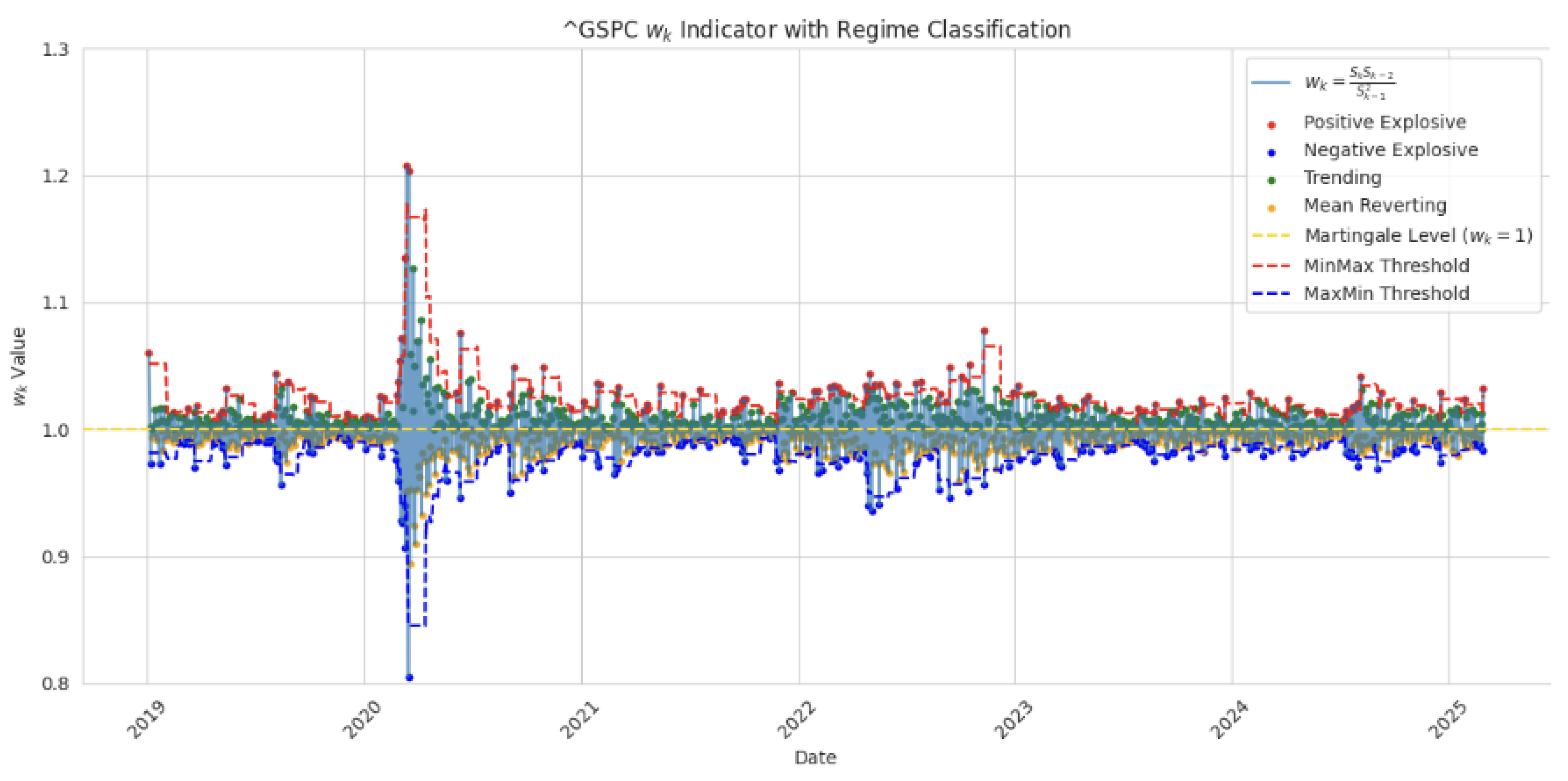
In Figure 1, we filter the data to create a map of martingale, trending, mean reverting, and explosive values of the S&P500.

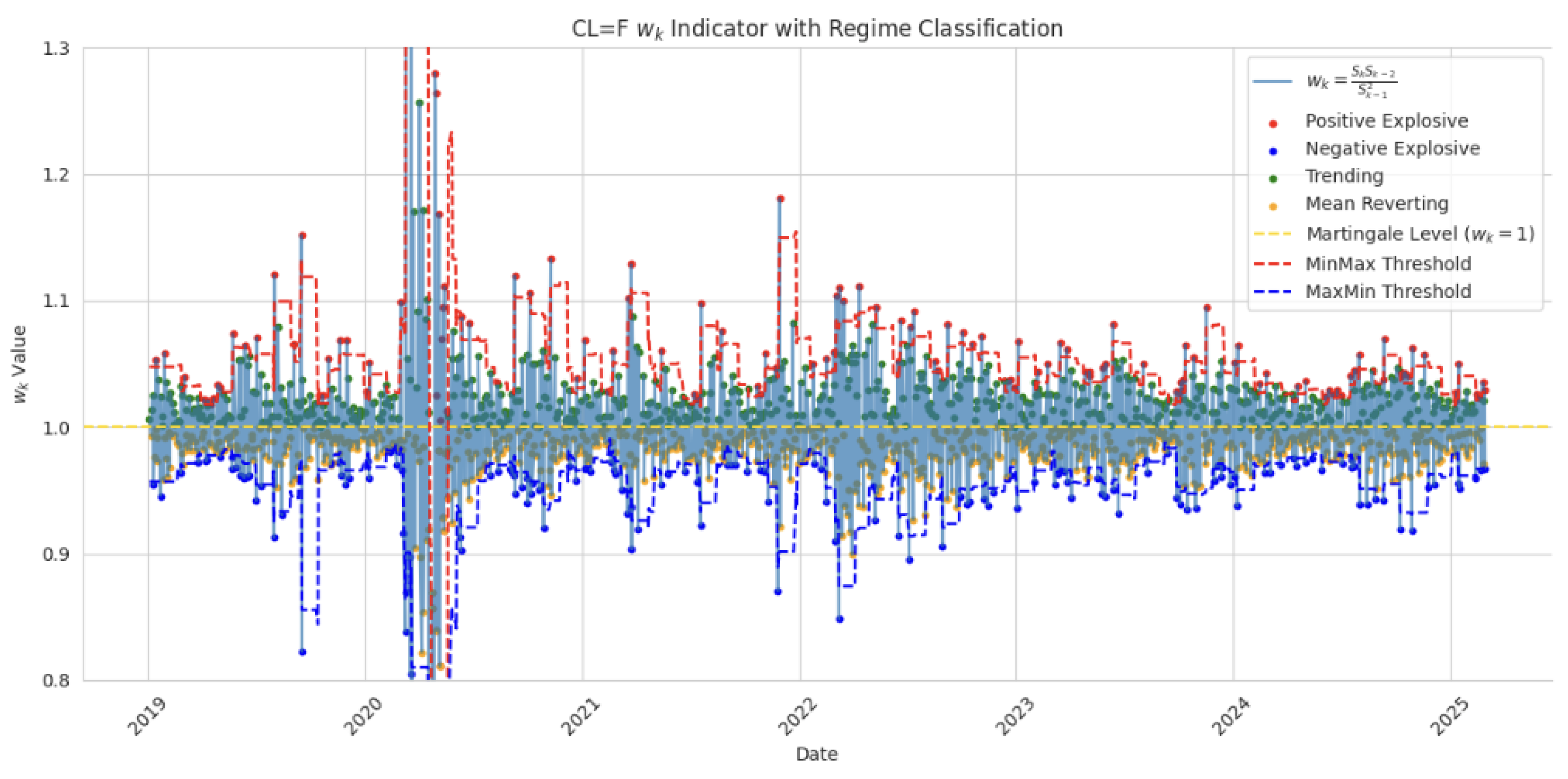
In Figure 2, we filter the data to create a map of martingale, trending, mean reverting, and explosive values of crude oil.

In Figure 3, we filter the data to create a map of martingale, trending, mean reverting, and explosive values of the 10-year US Treasury yield.

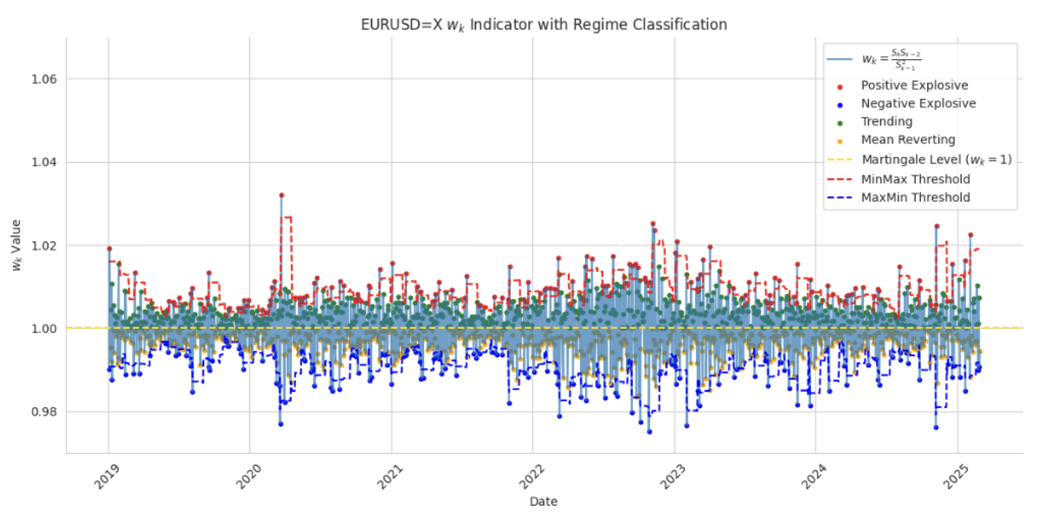
In Figure 4, we filter the data to create a map of martingale, trending, mean reverting, and explosive values of the EUR/USD exchange rate.

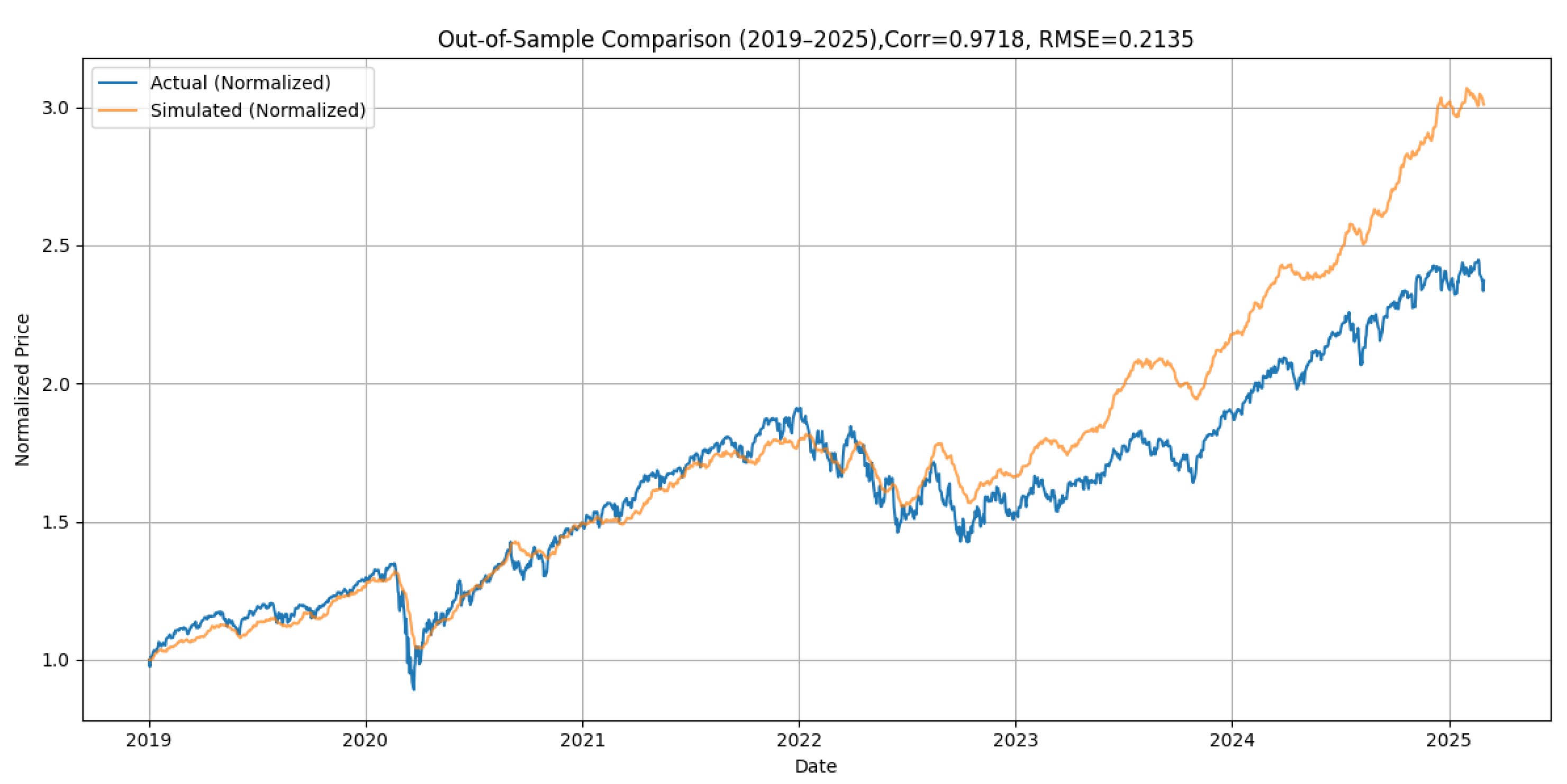
We evaluate the model based on five major financial instruments spanning equities, commodities, interest rates, cryptocurrencies, and foreign exchange rates. These include the S&P 500 Index (GSPC), crude oil prices (CL=F), the 10-year Treasury yield (TNX), Bitcoin (BTC-USD), and the EUR/USD exchange rate (EURUSD=X). For each case, the same model structure and calibration procedure are applied. All simulations are conducted over a six-year out-of-sample window (2019–2025). Since we performed out-of-sample comparison, we decided to extend our sample to March 2025. The macroeconomic uncertainty of the new US administration is now considered. using parameters estimated exclusively from data prior to 2019. This extended horizon allows us to test the model’s robustness without recalibration. As expected, the longer the model projects into the future without updating its parameters, the greater the divergence from actual market outcomes. Nevertheless, the model achieves remarkably strong performance across a range of assets.

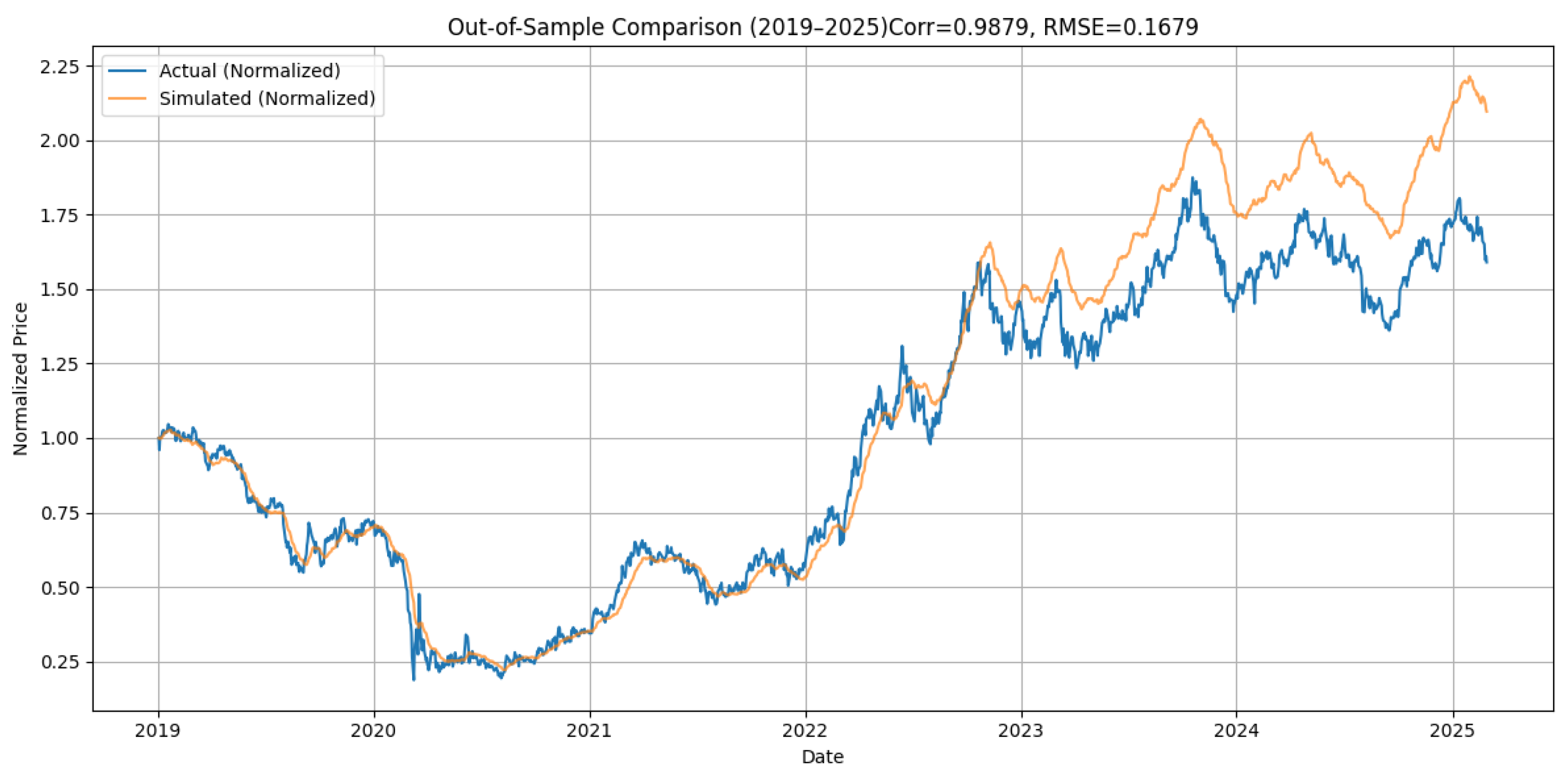
The model shows excellent predictive alignment for Bitcoin (see Figure 5), where explosive volatility and strong directional trends are mirrored closely by the simulated path.

Similarly, in the S&P 500 Index (see Figure 6), the simulation reproduces the equity market’s upward trajectory, including the COVID-19 shock and post-2020 bull run.

For the 10-year Treasury yield (see Figure 7), the model tracks interest rate cycles and trend shifts with impressive consistency.

Crude oil price presents a complex but well-captured cycle of collapse, rebound, and stabilization, where the model captures not only the directional momentum, but also much of the cyclical behavior (seeFigure 8).

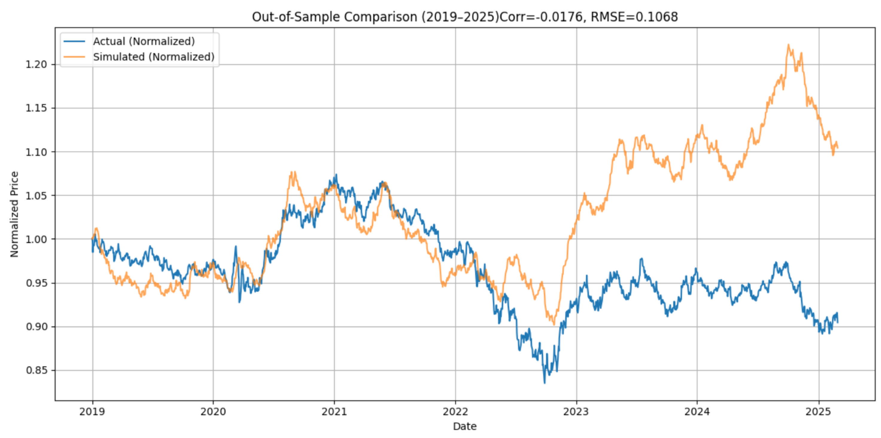
The EUR/USD exchange rate presents the greatest challenge due to its mean-reverting and policy-sensitive nature (see Figure 9).However, we observe that between 2019 and mid-2022, the model reproduces the actual path with exceptional precision. As we move forward in time without updating the parameters, the error grows with resulting deterioration in fit in the latter part of the sample, after significant structural changes in macroeconomic conditions, particularly the divergence in ECB and Fed policy post pandemic. These limitations are not faults of the model structure per se, but rather a consequence of using static, pre-2019 parameters for a system that evolved dramatically in later years.

Although the overall fit deteriorates after mid-2022, the model reproduces the price path of EUR/USD from 2019 to early 2022 with impressive accuracy. This initial alignment validates the relevance of our structural drift specification before exogenous macro shocks and interest rate divergences distort the dynamics.

Most modern AI and machine learning forecasting systems, including LSTMs, neural regressors, and hybrid models, also target levels rather than returns. This is largely because price levels are directly observable, whereas returns are derived quantities that can amplify noise or obscure structural features of the data. Forecasting levels enables models to better retain information related to long-term growth trends and volatility persistence. In line with this, the AREM in this paper forecasts price levels, not returns. Price levels are explicitly driven by latent volatility and embedded growth rates that determine the dynamic trajectory of prices across time. These structural drivers—rather than differenced returns—form the natural foundation for modeling historically dependent stochastic processes.

Our model yields a strikingly high percentage of correct predictions, ranging from 73% to 92%, in contrast to the 47% to 54% accuracy of naïve and moving average models.

We measure whether the model correctly anticipates the direction of price movement, i.e., whether the price increased when the model predicted an upward movement. Directional accuracy is especially appropriate in the context of level forecasting, where capturing turning points and directional shifts is more meaningful than predicting raw return magnitudes. Furthermore, when the level forecasts achieve such high out-of-sample correlation—97% for Bitcoin, 98% for the S&P500, and 98% for 10-year Treasury yields—it also implies that the derived return series would exhibit similarly high correlation with realized returns. In other words, if the model replicates the level path of an asset with high fidelity, it necessarily captures the directional movements and the relative return dynamics implied by that trajectory.

The empirical validity is evaluated through a rigorous out-of-sample framework extending from 2019 to 2025, using parameter estimates calibrated exclusively on pre-2019 data. This represents one of the most extensive multi-asset out-of-sample validation exercises in the literature. Among the reviewed studies, no study offers a comparably long and continuous out-of-sample evaluation spanning daily data across multiple asset classes and lasting up to six years as that implemented in this paper; while some works such as [21,24] perform robust out-of-sample validations, their horizons are notably shorter and often limited to equity returns or quarterly macro-indicators. Refs. [30,31] focus primarily on in-sample or short-horizon predictive regressions. Among the related studies employing forecasting methods across dynamic systems, we note the comparative study by [15], which contrasts classical mathematical models (SIR-type) with machine learning techniques in the context of COVID-19 spread prediction. Their analysis, focused on the Moscow region, evaluates short-term forecasts using multiple data-driven approaches, while their work highlights the potential of hybrid frameworks and explores modeling under uncertainty, the forecast horizon remains relatively limited—typically ranging from several days to a few weeks. Whereas Pavlyutin et al. emphasize model comparison under changing epidemic conditions, our work focuses on embedding historical dependence structurally and evaluating forecast accuracy in financial contexts subject to regime shifts and latent memory effects. In [32] emphasize volatility decomposition and connectedness, but do not provide out-of-sample forecast evaluation. Our results therefore offer a rare example of sustained model performance over six years and across diverse asset classes—including equities, interest rates, FX, oil, and cryptocurrency—using consistent calibration and structure. This out-of-sample robustness is a distinguishing feature of our approach, validating the structural memory captured in the adaptive regime-awareness in AREM.

To provide a more quantitative benchmark against prior research, we summarize directional accuracy figures in

Table 3. Extended comparison of forecasting models in the recent literature.

Study	Methodology	Accuracy/RMSE	Notes
This Paper AREM	Structural, orthogonality-aware model	73–93% (DA)	Multi-asset, 6-year out-of-sample
This Paper (Equation (17)	Recursive memory price simulation	High Correlation	Accurate path shape (price levels)
[21]	Structural break predictability test	70–85% (DA)	Stocks, rolling forecast
[24]	ML with return-sorted predictors	∼75% (DA)	Requires feature expansion
[23]	ML for inflation nowcasting	∼65–80%	Macroeconomic data
[27]	LSTM for crypto volatility	RMSE improved	Bitcoin-focused
[25]	Hybrid RNN + exponential smoothing	5–15% RMSE gains	Short-term forecasts
[33]	Idiosyncratic volatility (Fama-MacBeth)	~60%	Equities (cross-sectional)
[31]	Conditional skewness/kurtosis	~68%	U.S. equities
[34]	Frequency-domain Connectedness	Not reported	FX, bonds
[30]	Latent factor state-space model	~53–75%	International equities
[26]	Neural forecast meta-review	Mixed	Emphasis on scalability
[19]	Forecast breakdown tests	n/a	Detection, not prediction
[20]	Robust break detection	n/a	Model selection framework
[18]	FDA in Banach space	n/a	Functional data regressions

, drawing from recent papers addressing asset return predictability under various modeling assumptions. As shown, our AREM model delivers directional accuracy in the range of 73–93%, outperforming traditional models like Fama–MacBeth regressions [33], which average around 60%, and moment-based approaches such as [31], who report accuracies near 68% for U.S. equities. The frequency domain connectedness metrics of [34], while insightful on volatility transmission, do not explicitly report predictive statistics. Similarly, ref. [30] achieve an in sample $R^2$ 53%–75% using latent factor state-space models on international equity panels. The comparative advantage of our AREM framework lies in its ability to dynamically adapt to structural changes without requiring full state observability or restrictive moment assumptions. Overall, our empirical model stands favorably relative to both conventional econometric and modern ML-based alternatives.

To provide a comprehensive benchmark, Table 3 consolidates the predictive performance of our models with a broad range of recent forecasting approaches in the literature. This table includes both statistical and machine learning frameworks, spanning structural econometric models, regime-switching techniques, neural networks, and hybrid systems. Our AREM model exhibits directional accuracy between 73% and 93%, placing it at the upper end of the performance spectrum. It achieves exceptionally high out-of-sample correlation with realized price levels—97% for Bitcoin, 98% for the S&P500, and 98% for 10-year Treasury yields—indicating its robustness in replicating price trajectories. These results are particularly notable given the long out-of-sample window (2019–2025) and fixed pre-2019 calibration. It performs competitively or exceeds the standards established in the literature across multiple metrics and asset domains.

By contrast, studies such as [21,24] report accuracies in the range of 70–85%, with varying assumptions and data scopes. Traditional econometric models, like those in [31,33] generally deliver lower directional accuracy (60–68%), and are often limited by static factor structures or moment conditions. Machine learning methods, such as those explored by [23,25,27], achieve moderate-to-strong performance depending on the forecast horizon and asset class, but often lack interpretability. Other contributions, such as, [18,20,34] provide valuable theoretical or diagnostic tools but do not report explicit out-of-sample metrics.

4. Conclusions

This paper extends the foundational work of [4], who argued that the evolution of a stochastic process, $S_k$, is independent of its observable history under orthogonality assumptions. In their framework, the unobserved solution cannot be functionally linked to the observed data, implying a lack of duality and irreversibility in the underlying process. Under such conditions, history plays no role in the generation of future states, and predictability is fundamentally unattainable. Here, we have shown that under well-defined conditions in a reflexive Banach space, the evolution of the process $S_k$ is, indeed, historically dependent. Specifically, we demonstrate that for the majority of existing probabilistic configurations, three-quarters of all measures, the process exhibits dependence on its past. This historical dependence is formalized through the recursive relationship $S_k={\prod }_{j=-\infty }^k{\rho }_j·S_{k-1}$ and through orthogonality conditions derived from moment-generating functions of correlated sequences.

One important implication is that the dependence and independence alternatives for a general stochastic solution process would, indeed, depend on its known history. We argue that multidimensional integration has duality in reflexive Banach space if the solution obeys the functional central limit theorem and its error is between the limits of dilation and erosion. Hence, there is isomorphism for closed and semi-open intervals and the desired inner product to define the orthogonality conditions. Beyond that, the space is composed of countably additive and possibly finite measures endowed only with a measure and not a norm.

Another important result is the derivation of explicit orthogonality conditions, which enable the detection of whether the process $S_k$ behaves as a martingale ($w_k=1$) or deviates toward trend-following, mean-reverting, or explosive behavior ($w_k\ne 1$). These conditions support a regime classification framework embedded within the model, enhancing interpretability and predictive power. We further show that multidimensional integration has duality in reflexive Banach space if the solution satisfies a functional central limit theorem and its error is bounded between dilation and erosion. As such, the stochastic process is forecastable in most configurations, with explicit structural limits on predictability imposed by the geometry of the function space.

Duality, as established in the reflexive Banach space framework, plays a fundamental role in enhancing the model’s robustness. When the observed sequence lies in a space isomorphic to that of the unobserved process, it inherits essential topological properties—reflexivity, completeness, and convexity—which ensure that forecastable structure is preserved. This duality forms the theoretical basis for the model’s capacity to extract meaningful information from noisy or incomplete observations.

Empirically, AREM demonstrates substantial gains in predictive power relative to moving average and naïve models. Across assets with vastly different characteristics—including the S&P 500, Bitcoin, and US Treasury bonds—AREM achieves directional accuracy between 73% and 93%, outperforming traditional benchmarks that falter in the presence of non-stationarity and heavy tails. The orthogonality and duality framework embedded in the model is instrumental in capturing and adapting to dynamic changes in the data-generating process. The dual approach strengthens our understanding of historical dependence, structural predictability, and their implications for forecasting under incomplete information.

The duality-based stochastic process model presented in this paper offers significant potential for enhancing cybersecurity in financial systems. By establishing a rigorous mapping between observable financial data and latent stochastic drivers, our model facilitates structural auditability and anomaly detection. This is particularly pertinent given the increasing sophistication of cyber threats targeting financial institutions. For instance, the National Institute of Standards and Technology (NIST) has emphasized the need for robust defenses against adversarial machine learning attacks, which can compromise the integrity of financial models [35]. Additionally, recent studies have highlighted the vulnerability of financial systems to advanced persistent threats (APTs) and the necessity of mathematical models for effective cyber risk management [36]. Our model’s capacity to detect deviations from expected stochastic behavior can serve as an early warning mechanism against such threats, thereby reinforcing the cybersecurity infrastructure of financial institutions. Recent work by [37] proposes a two-stage stochastic programming model for cybersecurity investment that incorporates attacker behavior, government intelligence, and firm-level safeguards. Their framework mirrors our approach by embedding long-memory dependence and recursive decision-making under uncertainty. Moreover, studies such as [38,39] emphasize that cyber–physical and network security systems require robust mathematical models that accommodate stochastic attacks and degeneracy in observed intrusion patterns. These conditions align with the orthogonality and reflexivity principles central to our modeling strategy. The ability of our model to detect breaks in structural correspondence—when the observed process $S_k$ deviates from its latent generator—is analogous to identifying anomalous states or adversarial threats in a cybersecurity environment. This suggests that our theoretical tools can contribute to dynamic detection, resilience modeling, and investment optimization in the cybersecurity domain, particularly in high-frequency financial systems and adversarial machine learning contexts.