
A Semi-Parametric KDE-GPD Model for Earthquake Magnitude Analysis

Abstract
1. Introduction
2. Semi-Parametric Mixture Model
3. Parameter Estimation of the Semi-Parametric Mixture Model
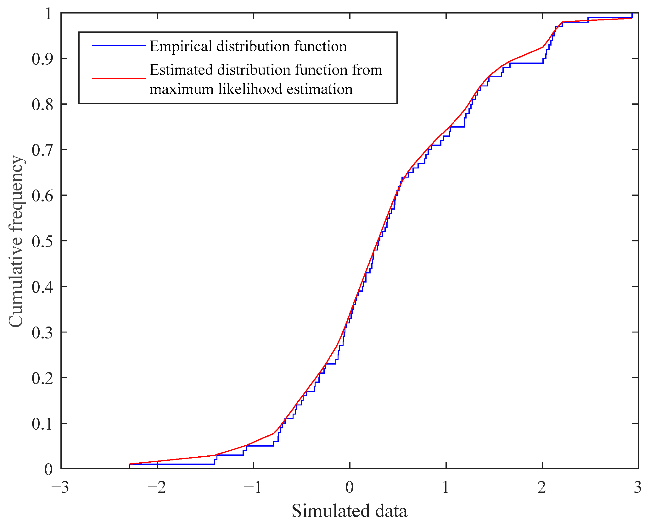
3.1. MLE of Parameters
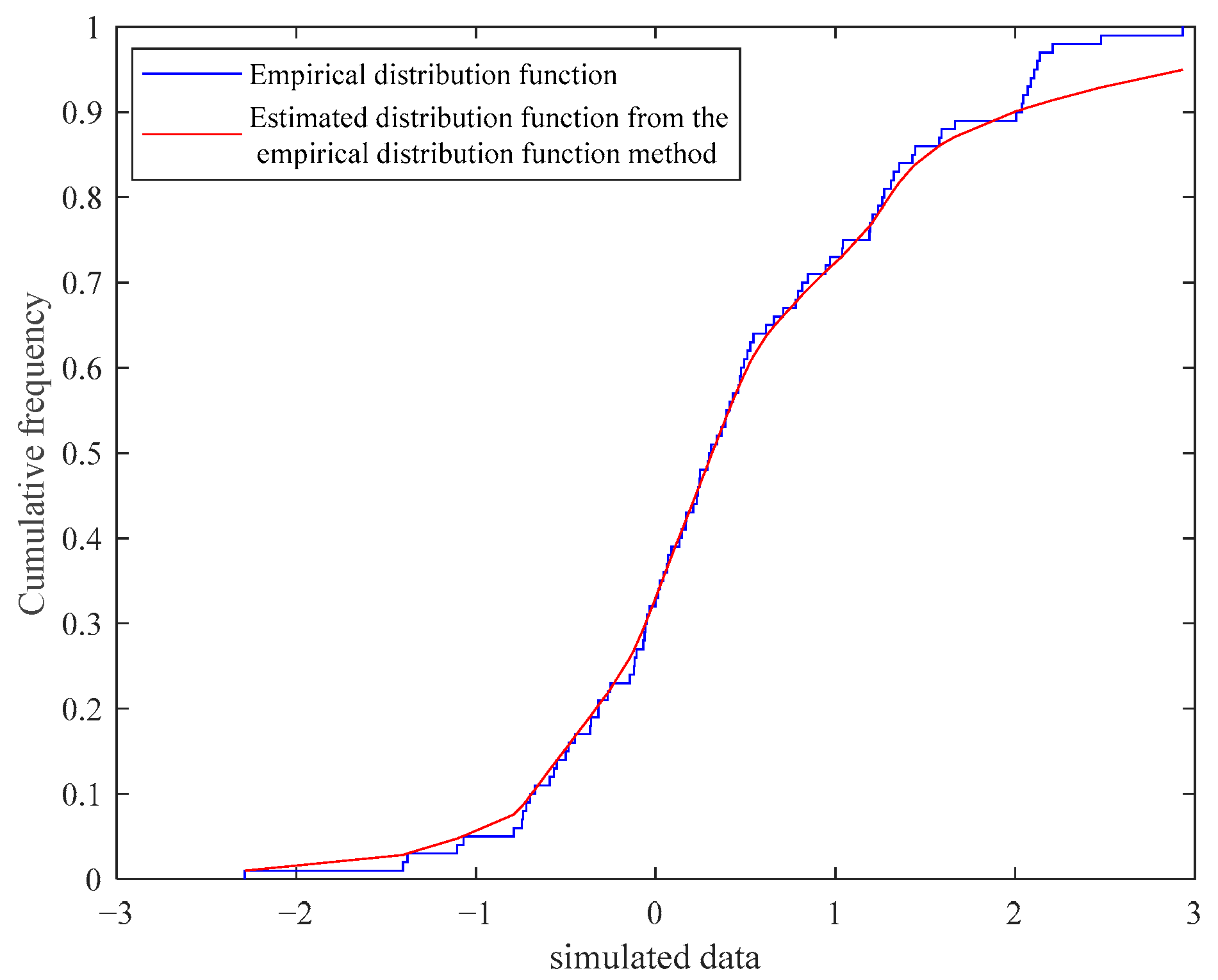
3.2. Parameter Estimation Method Based on the EDF
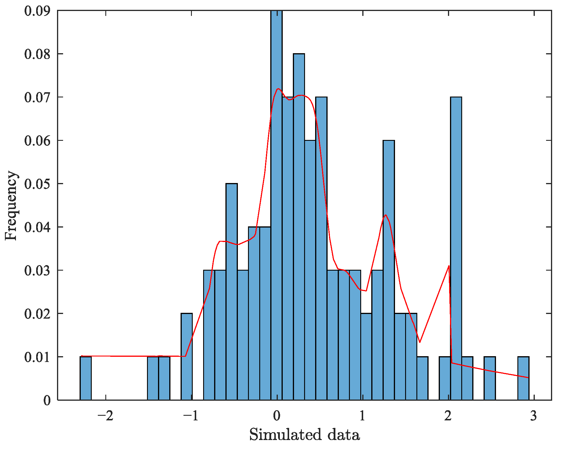
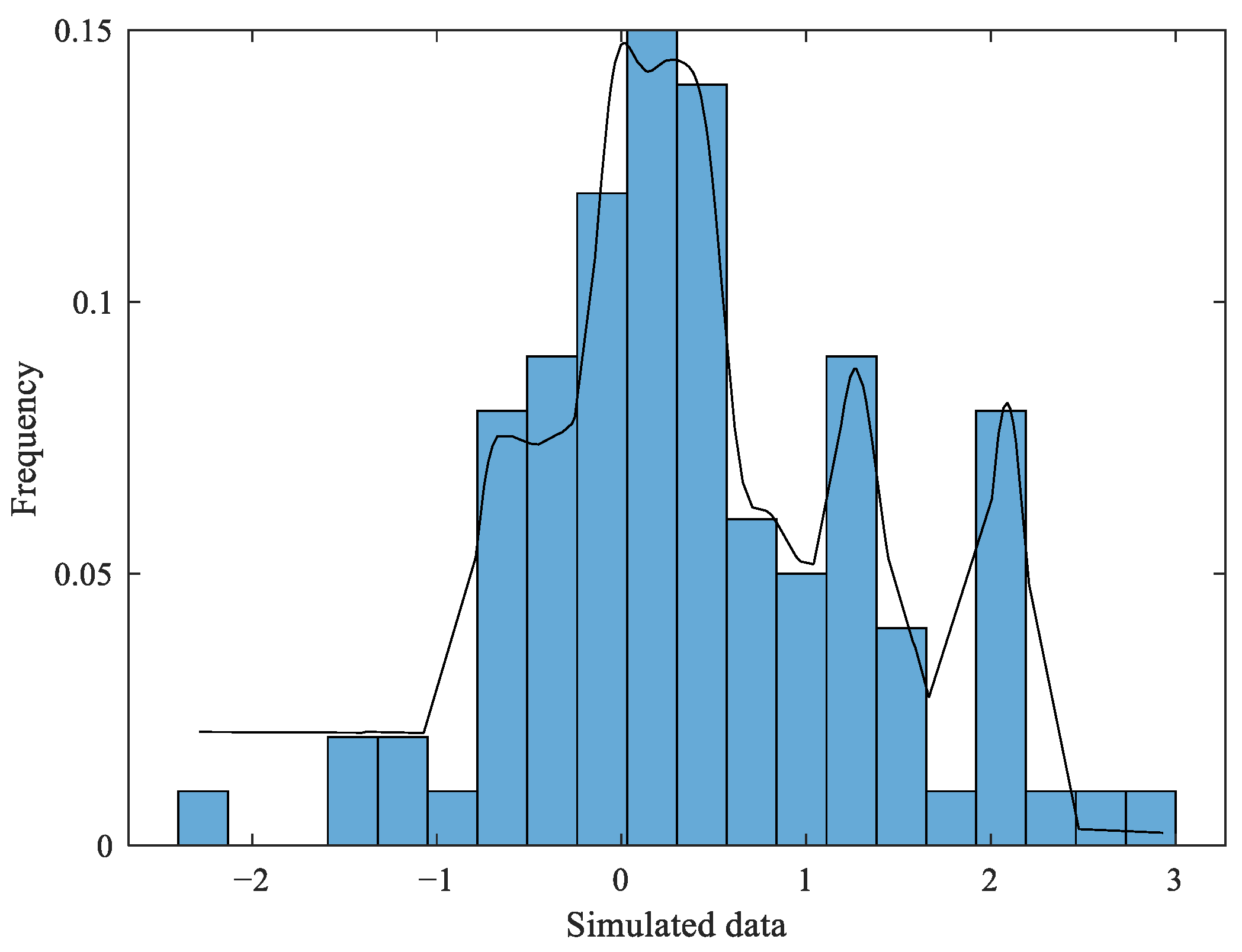
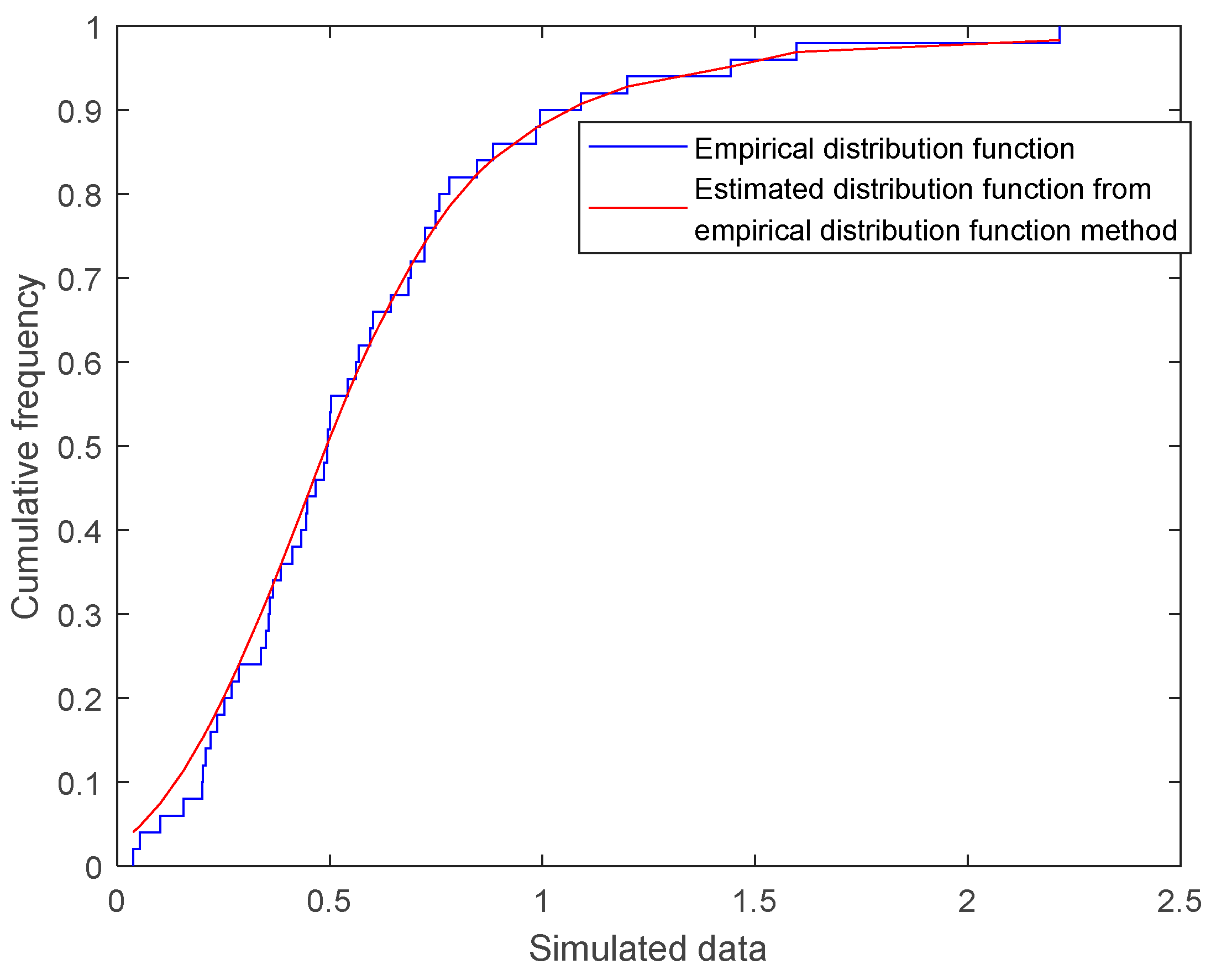
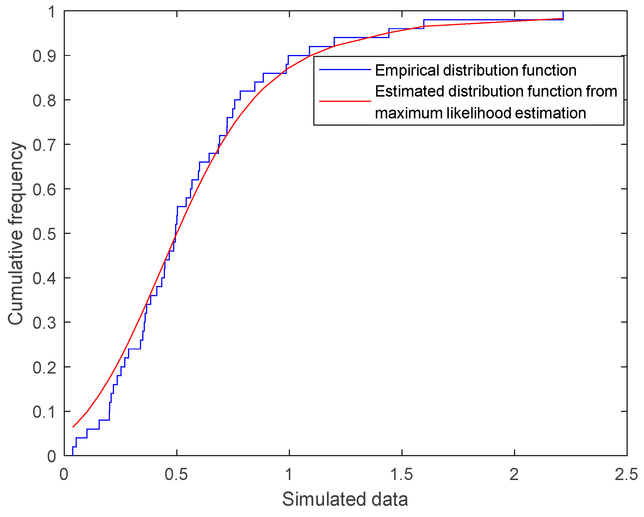
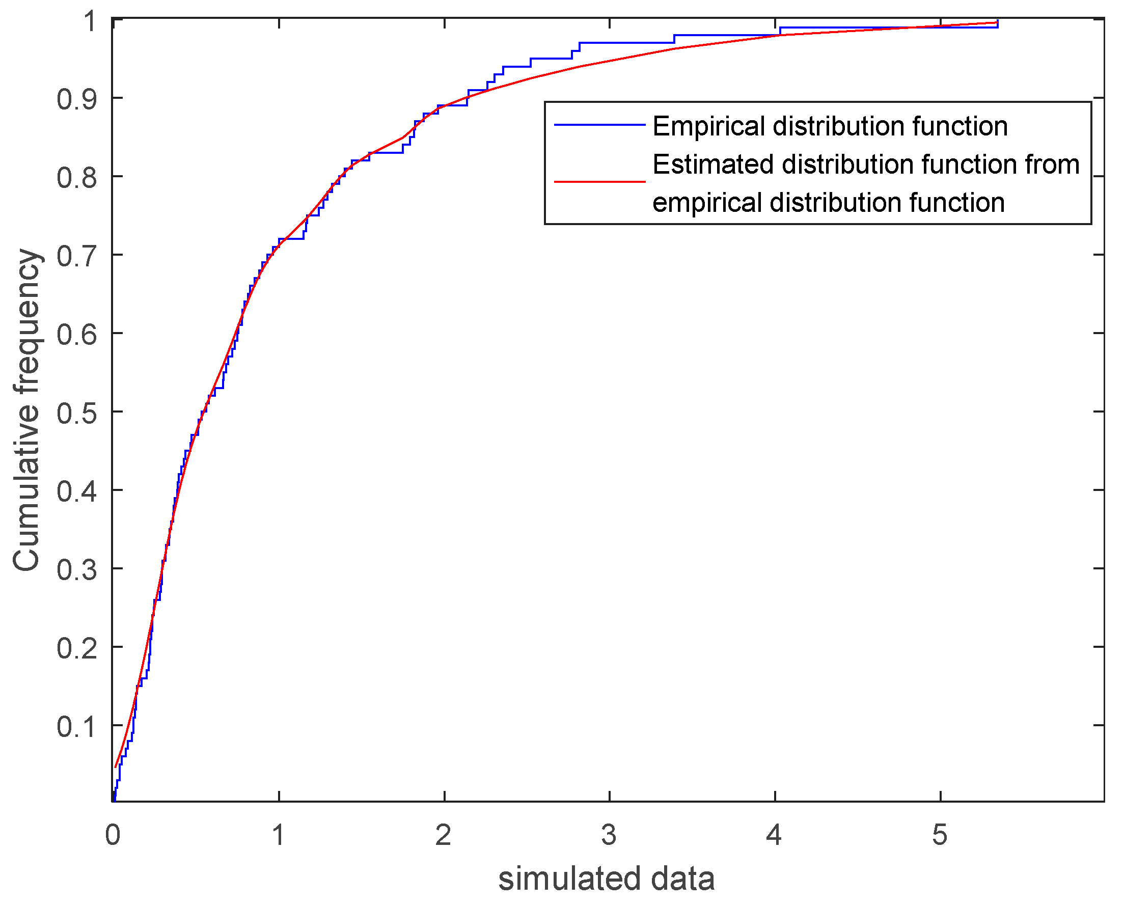
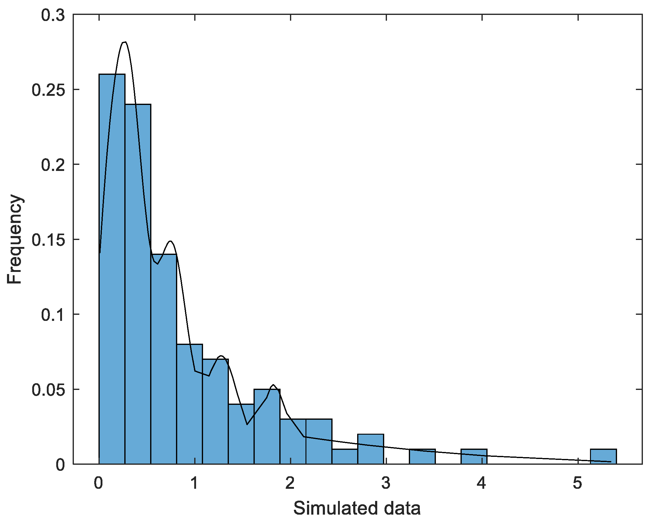
4. Simulation of Parameter Estimation for Semi-Parametric Mixture Models
- Normal (shape = 1, scale = 4) + GPD.
- Weibull (shape = 1.5, scale = 2) + GPD.
- Gamma (shape = 1, scale = 2) + GPD.
5. Statistical Characteristic Analysis of Seismic Magnitude Data in the Eastern Bayan Har Block
5.1. Data Statistics
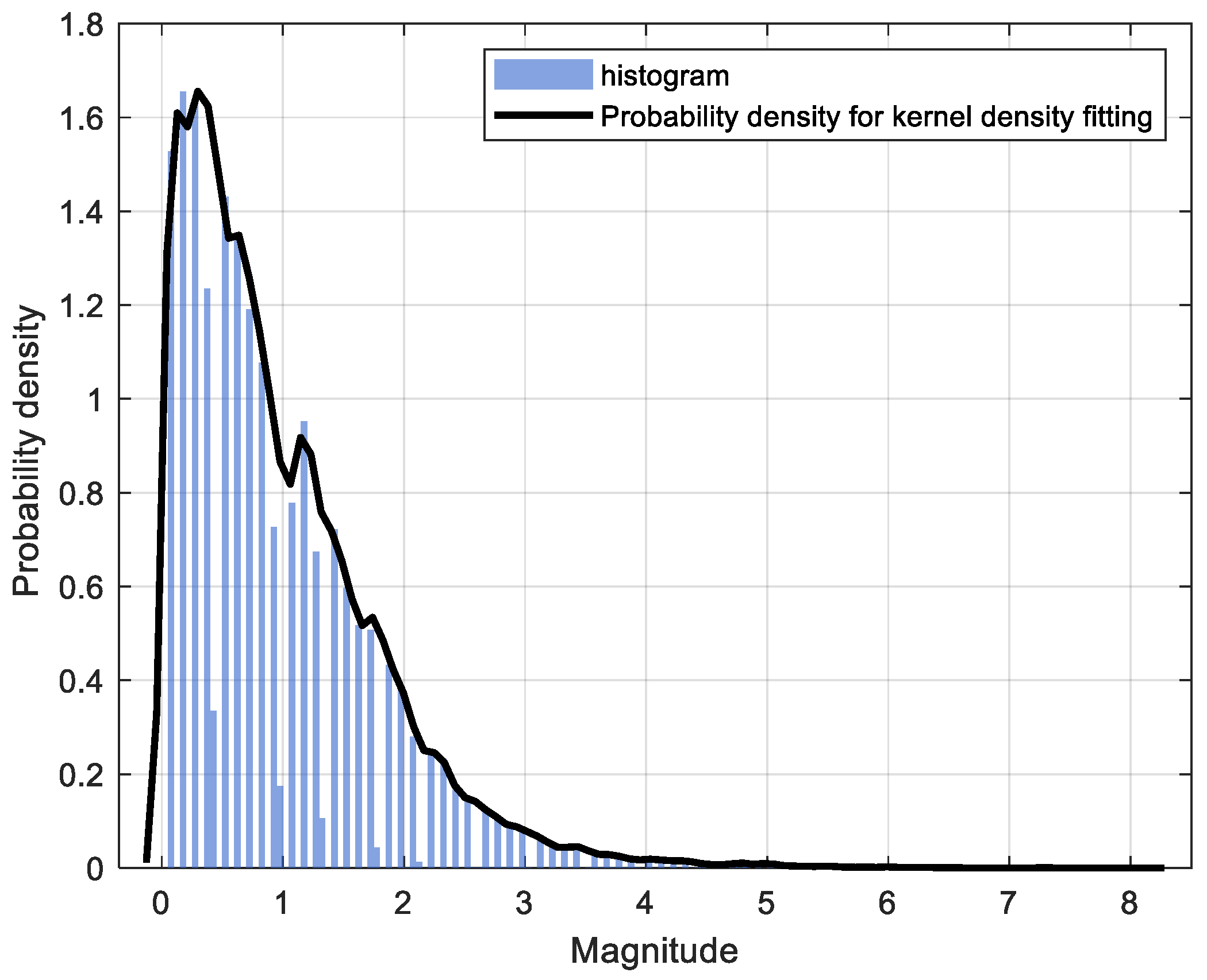
5.2. Nonparametric KDE of the Data
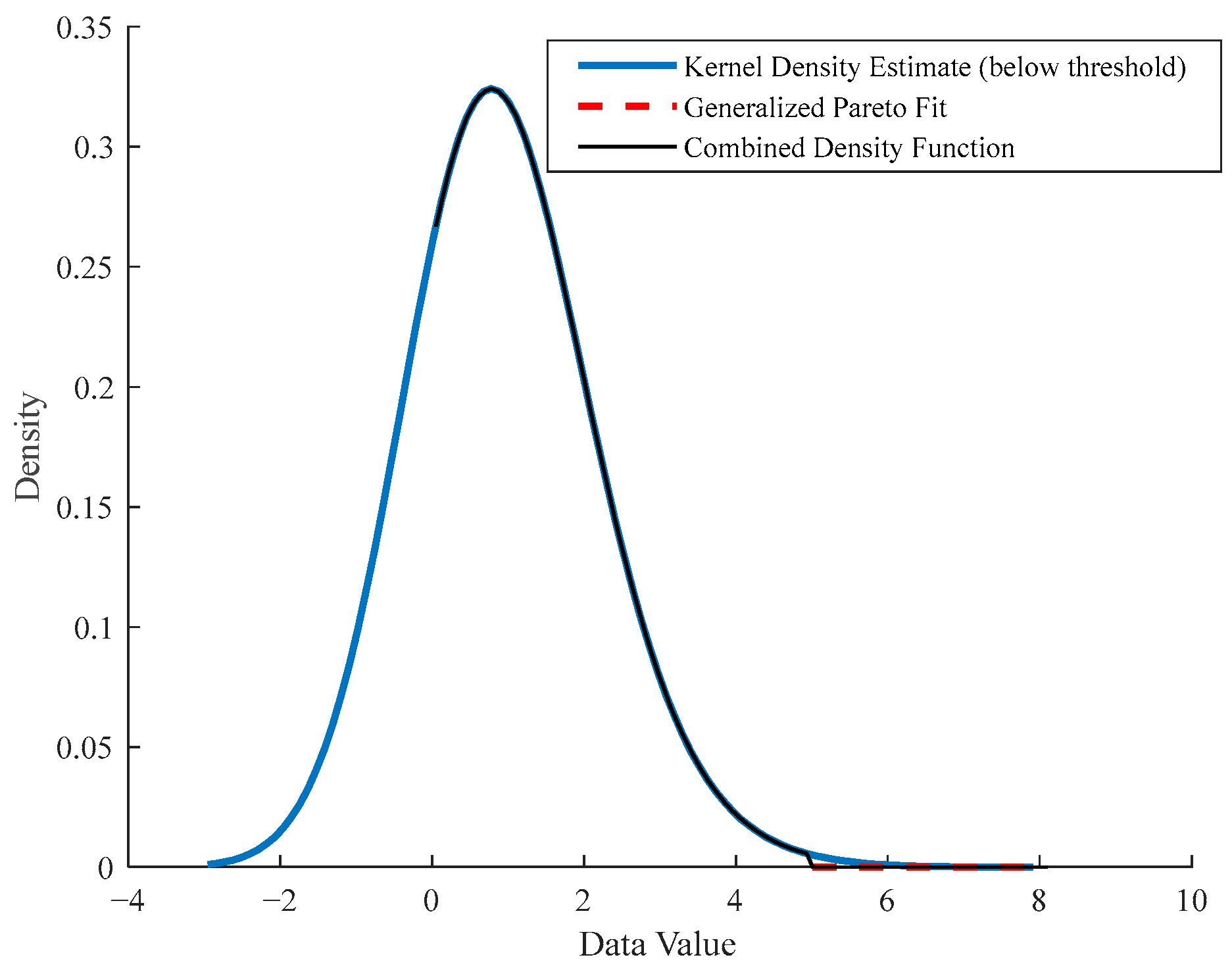
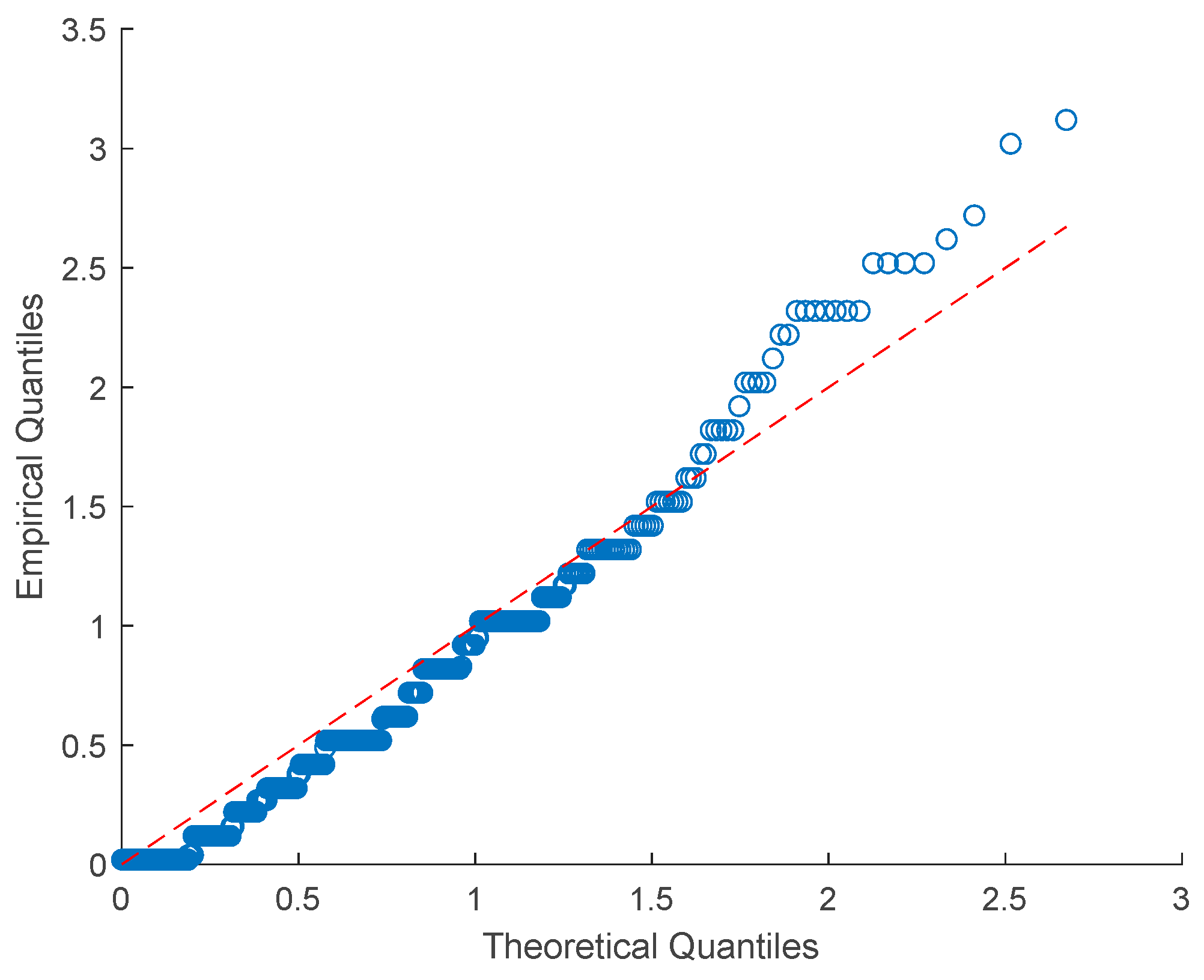
5.3. Data Fitting Using the Semi-Parametric Mixture Model
6. Conclusions
Author Contributions
Funding
Data Availability Statement
Conflicts of Interest
References
- Gutenberg, B.; Richter, C.F. Magnitude and energy of earthquakes. Ann. Geophys. 2010, 53, 7–12. [Google Scholar] [CrossRef]
- Dutfoy, A. Estimation of tail distribution of the annual maximum earthquake magnitude using extreme value theory. Pure Appl. Geophys. 2019, 176, 527–540. [Google Scholar] [CrossRef]
- Dutfoy, A. Earthquake recurrence model based on the generalized Pareto distribution for unequal observation periods and imprecise magnitudes. Pure Appl. Geophys. 2021, 178, 1549–1561. [Google Scholar] [CrossRef]
- Zhang, Y.F.; Zhao, Y.B.; Ren, Q.Q. Seismic risk in the east of the Bayan Har block based on the POT model. Geomat. Nat. Hazards Risk 2022, 13, 2697–2711. [Google Scholar] [CrossRef]
- Frigessi, A.; Haug, O.; Rue, H. A dynamic mixture model for unsupervised tail estimation without threshold selection. Extremes 2002, 5, 219–235. [Google Scholar] [CrossRef]
- Mendes, B.V.d.M.; Lopes, H.F. Data driven estimates for mixtures. Comput. Stat. Data Anal. 2004, 47, 583–598. [Google Scholar] [CrossRef]
- Behrens, C.N.; Lopes, H.F.; Gamerman, D. Bayesian analysis of extreme events with threshold estimation. Stat. Model. 2003, 4, 227–244. [Google Scholar] [CrossRef]
- Zhang, Y.; Wang, F.; Zhao, Y. Statistical characteristics of earthquake magnitude based on the composite model. AIMS Math. 2024, 9, 607–624. [Google Scholar] [CrossRef]
- Heckman, J.; Singer, B. A method for minimizing the impact of distributional assumptions in econometric models for duration data. Econometrica 1984, 52, 271–320. [Google Scholar] [CrossRef]
- Wang, Y.; Chee, C.-S. Density estimation using non-parametric and semi-parametric mixtures. Stat. Model. 2012, 12, 67–92. [Google Scholar] [CrossRef]
- Fienberg, S.E.; Bromet, E.J.; Follmann, D.; Lambert, D.; May, S.M. Longitudinal analysis of categorical epidemiological data: A study of Three Mile Island. Environ. Health Perspect. 1985, 63, 241–248. [Google Scholar] [CrossRef] [PubMed]
- Follmann, D.A.; Lambert, D. Generalizing logistic regression by nonparametric mixing. J. Amer. Statist. Assoc. 1989, 84, 295–300. [Google Scholar] [CrossRef]
- Davies, R.B. Nonparametric control for residual heterogeneity in modelling recurrent behaviour. Comput. Stat. Data Anal. 1993, 16, 143–160. [Google Scholar] [CrossRef]
- Hall, P.; Zhou, X.-H. Nonparametric estimation of component distributions in a multivariate mixture. Ann. Stat. 2003, 31, 201–224. [Google Scholar] [CrossRef]
- Hall, P.; Neeman, A.; Pakyari, R.; Elmore, R. Nonparametric inference in multivariate mixtures. Biometrika 2005, 92, 667–678. [Google Scholar] [CrossRef]
- Bordes, L.; Delmas, C.; Vandekerkhove, P. Semiparametric estimation of a two-component mixture model where one component is known. Scand. J. Stat. 2006, 33, 733–752. [Google Scholar] [CrossRef]
- Hunter, D.R.; Wang, S.; Hettmansperger, T.P. Inference for mixtures of symmetric distributions. Ann. Stat. 2007, 35, 224–251. [Google Scholar] [CrossRef]
- Song, S.; Nicolae, D.L.; Song, J. Estimating the mixing proportion in a semiparametric mixture model. Comput. Stat. Data Anal. 2010, 54, 2276–2283. [Google Scholar] [CrossRef]
- Bordes, L.; Kojadinovic, I.; Vandekerkhove, P. Semiparametric estimation of a mixture of two linear regressions where one component is known. Electron. J. Stat. 2013, 7, 2603–2644. [Google Scholar] [CrossRef]
- Bordes, L.; Vandekerkhove, P. Semiparametric two-component mixture model with a known component: An asymptotically normal estimator. Math. Methods Stat. 2010, 19, 22–41. [Google Scholar] [CrossRef]
- Xiang, S.; Yao, W.; Wu, J. Minimum profile Hellinger distance estimation for a semiparametric mixture model. Can. J. Stat. 2014, 42, 246–267. [Google Scholar] [CrossRef]
- Xiang, S.; Yao, W.; Yang, G. An overview of semiparametric extensions of finite mixture models. Stat. Sci. 2019, 34, 391–404. [Google Scholar] [CrossRef]
- Huang, M.; Wang, S.; Wang, H.; Jin, T. Maximum smoothed likelihood estimation for a class of semiparametric pareto mixture densities. Stat. Interface 2018, 11, 31–40. [Google Scholar] [CrossRef]
- Young, D.; Hunter, D. Mixtures of regressions with predictor-dependent mixing proportions. Comput. Stat. Data Anal. 2010, 54, 2253–2266. [Google Scholar] [CrossRef]
- Huang, M.; Yao, W. Mixture of regression models with varying mixing proportions: A semiparametric approach. J. Am. Stat. Assoc. 2012, 107, 711–724. [Google Scholar] [CrossRef]
- Macdonald, A.; Scarrott, C.; Lee, D.; Darlow, B.; Reale, M.; Russell, G. A flexible extreme value mixture model. Comput. Stat. Data Anal. 2011, 55, 2137–2157. [Google Scholar] [CrossRef]
- Pommeret, D.; Vandekerkhove, P. Semiparametric density testing in the contamination model. Electron. J. Stat. 2019, 13, 4743–4793. [Google Scholar] [CrossRef]
- Yin, A.; Yuan, A. Multi-dimensional classification with semiparametric mixture model. Stat. Interface 2020, 13, 347–359. [Google Scholar] [CrossRef]
- Tan, X.; Yan, M. Semi-parametric density estimation method based on regular penalty. J. Chongqing Technol. Bus. Univ. Chin. 2025, 42, 1–9. [Google Scholar]
- Martins-Ferreira, T.; Sampaio, A.F.; Figueiredo, R.; Lopes, A.R.; Reis, M.T.; Fortes, C.J.E.M.; Silva, R. Hybrid transformer-exceedance models for compound flooding. Nat. Hazards Earth Syst. Sci. 2024, 24, 801–817. [Google Scholar]
- Chen, Y.; Zhang, R. Adaptive Bayesian threshold selection for extreme value mixtures. Technometrics 2023, 65, 511–525. [Google Scholar]
- Vinayan, S.; Kumar, V.S.; Sajeev, R. Variabilities in the estimate of 100-year return period wave height in the Indian shelf seas. J. Oceanogr. 2024, 80, 377–391. [Google Scholar] [CrossRef]
- Liu, Q.; Zhou, H. Massively parallel continuity constraints for semi-parametric extremes. Comput. Stat. Data Anal. 2025, 189, 107831. [Google Scholar]
- Kinnison, R.R. Applied Extreme Value Statistics, 1st ed.; Battelle Press: Columbus, OH, USA, 1985; pp. 132–166. [Google Scholar]
- Epanechnikov, V.A. Non-parametric estimation of a multivariate probability density. Theory Probab. Appl. 1969, 14, 153–158. [Google Scholar] [CrossRef]
- Gramacki, A. Kernel density estimation outperforms orthogonal series and maximum entropy methods. In Nonparametric Kernel Density Estimation and Its Computational Aspects, 1st ed.; Springer International Publishing: Cham, Switzerland, 2018; pp. 23–47. [Google Scholar]
- Sheather, S.J.; Jones, M.C. A reliable data-based bandwidth selection method for kernel density estimation. J. R. Stat. Soc. Ser. B 1991, 53, 683–690. [Google Scholar] [CrossRef]
- Kamer, Y.; Hiemer, S. Data-driven spatial b value estimation with applications to California seismicity. J. Geophys. Res. Solid Earth 2015, 120, 2601–2618. [Google Scholar] [CrossRef]
- Silverman, B.W. Density Estimation for Statistics and Data Analysis; Chapman and Hall: London, UK, 1986; pp. 68–96. [Google Scholar]
- Wand, M.P.; Jones, M.C. Multivariate plug-in bandwidth selection. Comput. Stat. Data Anal. 1994, 17, 97–116. [Google Scholar]
- Tancredi, A.; Anderson, C.; O’Hagan, A. Accounting for threshold uncertainty in extreme value estimation. Extremes 2006, 9, 87–106. [Google Scholar] [CrossRef]
- Habbema, J.; Hermans, J.; van den Broek, K. A stepwise discriminant analysis program using density estimation. In Compstat; Bruckmann, G., Ed.; Physica-Verlag: Vienna, Austria, 1974; pp. 101–110. [Google Scholar]
- Duin, R.P.W. On the choice of smoothing parameters for Parzen estimators of probability density functions. IEEE Trans. Comput. C 1976, 25, 1175–1179. [Google Scholar] [CrossRef]
- Bowman, A.W. A note on consistency of the kernel method for the analysis of categorical data. Biometrika 1980, 67, 682–684. [Google Scholar] [CrossRef]
- Bowman, A.W. An alternative method of cross-validation for the smoothing of density estimates. Biometrika 1984, 71, 353–360. [Google Scholar] [CrossRef]
- Chen, L.; Liu, J.; Chen, Y.; Chen, L.S. Aftershock deletion in seismicity analysis. Acta Geophys. Sin. 1998, 41 (Suppl. 1), 244–252. (In Chinese) [Google Scholar]


| Parameter estimations by EDF | 0.6005 | 2.0153 | −0.2358 | 1.4802 |
| Standard deviation | 0.0052 | 0.0211 | 0.0498 | 0.0001 |
| Confidence interval (confidence level ) | (0.6000, 0.6001) | (1.752, 2.0664) | (−0.3750, −0.0589) | (1.3800, 1.5816) |
| Parameters by MLE | 0.3817 | 2.0053 | −0.2388 | 1.4901 |
| Standard deviation | 0.1213 | 0.0142 | 0.0388 | 0.0008 |
| Confidence interval (confidence level ) | (0.1035, 0.5811) | (1.300, 2.1438) | (−0.3419, 0.1207) | (1.331, 1.6734) |
| Parameter estimations by EDF | 0.6235 | 2.0003 | −0.1958 | 1.9802 |
| Standard deviation | 0.1241 | 0.0002 | 0.0498 | 0.1950 |
| Confidence interval (confidence level ) | (0.1003, 0.8005) | (1.8725, 2.0346) | (0.2975, 0.1018) | (1.2943, 2.2473) |
| Parameters by MLE | 0.7482 | 2.003 | −0.2080 | 1.7744 |
| Standard deviation | 0.1774 | 0.0142 | 0.0247 | 0.0877 |
| Confidence interval (confidence level ) | (0.1203, 0.8011) | (2.0064, 2.2438) | (−0.3419, −0.1007) | (1.3351, 1.8281) |
| Parameter estimations by EDF | 0.1001 | 2.0051 | −0.2463 | 1.4901 |
| Standard deviation | 0.0005 | 0.0124 | 0.0235 | 0.0430 |
| Confidence interval (confidence level ) | (0.1001, 0.80121) | (1.5764, 2.5995) | (−0.2803, 0.1484) | (1.3802, 1.5682) |
| Parameters by MLE | 0.1072 | 2.0235 | −0.2176 | 1.4880 |
| Standard deviation | 0.0141 | 0.0507 | 0.0683 | 0.0295 |
| Confidence interval (confidence level ) | (0.1103, 0.6012) | (1.7003, 2.3644) | (−0.1504, −0.0146) | (1.3213, 1.6180) |
| Minimum | Maximum | Mean | First Quartile (Q1) | Third Quartile (Q3) | Variance | Skewness | Kurtosis |
|---|---|---|---|---|---|---|---|
| 0.0500 | 8.1000 | 0.9617 | 0.3900 | 1.4100 | 0.6575 | 1.5523 | 6.7771 |
| Models | ||||
|---|---|---|---|---|
| KDE | 0.0591 | |||
| Semi-parametric mixture model (KDE-GPD) | 1.0001 | 4.9801 | −0.2021 | 0.7514 |
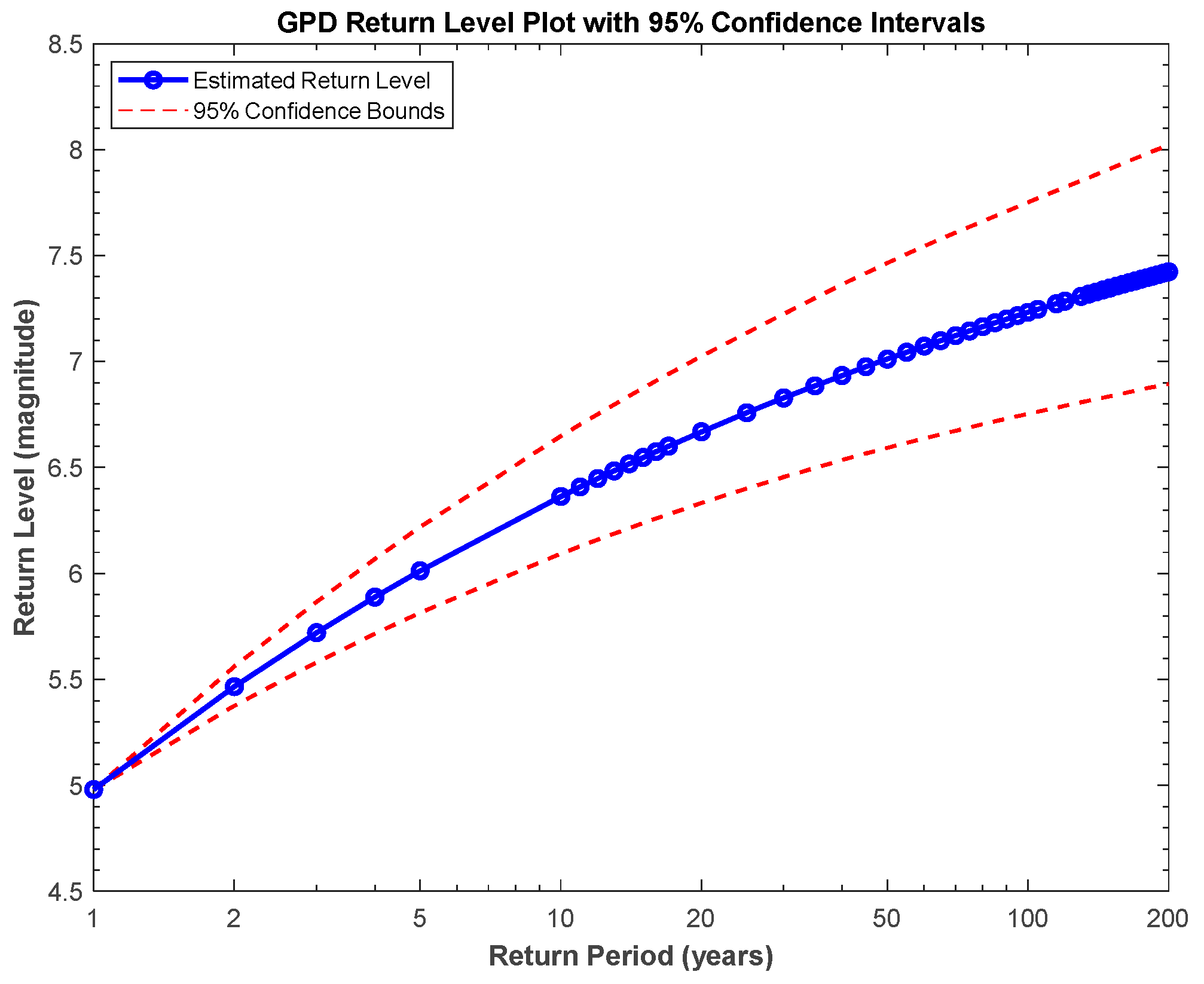
| Return Period (Years) | Return Level |
|---|---|
| 10 | 6.3635 |
| 20 | 6.6687 |
| 30 | 6.8283 |
| 50 | 7.0117 |
| 60 | 7.0727 |
| 80 | 7.1645 |
| 100 | 7.2322 |
Disclaimer/Publisher’s Note: The statements, opinions and data contained in all publications are solely those of the individual author(s) and contributor(s) and not of MDPI and/or the editor(s). MDPI and/or the editor(s) disclaim responsibility for any injury to people or property resulting from any ideas, methods, instructions or products referred to in the content. |
© 2025 by the authors. Licensee MDPI, Basel, Switzerland. This article is an open access article distributed under the terms and conditions of the Creative Commons Attribution (CC BY) license (https://creativecommons.org/licenses/by/4.0/).
Share and Cite
Zhang, Y.; Zhao, Y.; Wang, F. A Semi-Parametric KDE-GPD Model for Earthquake Magnitude Analysis. Mathematics 2025, 13, 2003. https://doi.org/10.3390/math13122003
Zhang Y, Zhao Y, Wang F. A Semi-Parametric KDE-GPD Model for Earthquake Magnitude Analysis. Mathematics. 2025; 13(12):2003. https://doi.org/10.3390/math13122003
Chicago/Turabian StyleZhang, Yanfang, Yibin Zhao, and Fuchang Wang. 2025. "A Semi-Parametric KDE-GPD Model for Earthquake Magnitude Analysis" Mathematics 13, no. 12: 2003. https://doi.org/10.3390/math13122003
APA StyleZhang, Y., Zhao, Y., & Wang, F. (2025). A Semi-Parametric KDE-GPD Model for Earthquake Magnitude Analysis. Mathematics, 13(12), 2003. https://doi.org/10.3390/math13122003