Abstract
Piezoelectric actuators are commonly used in high precision, micro-displacement applications. However, nonlinear phenomena, like hysteresis, may reduce their performance. This article compares several control approaches—based on the combination of sliding mode control and artificial neural networks—for coping with these nonlinearities and improving actuator positioning accuracy and robustness. In particular, it discusses the application of diverse order sliding mode control techniques, such as conventional, twisting algorithms, super-twisting algorithms, and the prescribed convergence law, in combination with artificial neural networks. Moreover, it validates experimentally, with a commercial piezoelectric actuator, the application of these control structures using a dSPACE 1104 controller board. Finally, it evaluates the computational time consumption for the control strategies presented. This work intends to guide the designers of PEA commercial applications to select the best control algorithm and identify the hardware requirements.
MSC:
93-08; 93-10; 93-05
1. Introduction
The manipulation and observation at atomic perspectives have been improved in the last 30 years with the improvements of microelectromechanics (MEMS) [1]. These allowed advances in fields such as aerospace or biology [2,3]. Nevertheless, MEMS are conditional on small devices for precise movements, which are dependent on micro/nano actuators [4]. Piezoelectric actuators (PEA) are commonly used in these roles because of their capacity to produce micro-displacements with high precision and even with loads due to their stiffness [5].
Piezoelectric materials generate an electric charge when mechanical stress or deformation is applied to them, a phenomenon known as the piezoelectric effect [6]. In the same way, these materials are stretched when a voltage is applied, which is known as the inverse piezoelectric effect [7]. This last effect is the one used for PEAs, and theoretically, it is produced as a consequence of the noncentrosymmetric atomic arrangement in a lattice; thus, an induced voltage in the material creates electrostatic forces in the atoms, and the lattice will extend or compress [8]. Hence, when a voltage is applied, the lattice expands, which causes an increment in the material size. Nevertheless, this polarization has a major downside, which is related to the effect known as hysteresis, which appears during the strain response and is also associated with the movement of the domain walls [9]. The latter-mentioned concept is known as planar defects in piezoelectrics, which are linked with pole reorientation and contribute to the material properties [10].
At the macroscopic level, hysteresis is a meaningful effect to be reduced since it induces instabilities and inaccuracies in PEAs [11]. From the point of view of material engineering, the hysteresis can be diminished when a redesign in the structure is performed. This implies that materials need to be harder but at the cost of reducing the Curie temperature, the value at which the piezoelectric properties are weak [12]. According to Dragan Damjanovic, hysteresis can also be decreased through an active control system, provided that the physical properties of the PEA are well understood [13].
Linear schemes can be an early approach to designing compensation for the hysteresis in PEAs. Mainly, proportional–integral–derivative (PID) controllers have been used widely for innovation and comparison of advanced proposals. Han et al. analyzed a complex fast steering mirror system that was driven by PEAs, where they embedded a PID due to its simplicity [14]. Experiments showed that the rotational precision achieved was in the required design range. On the other hand, another method reviewed is the linear quadratic Gaussian (LQG) controller, which has been implemented by the authors of [15]. In this research, they studied an active vibration isolation control, which is a common application of PEAs due to their fast response. The design was combined with a loop transfer recovery (LTR) in order to retrieve properties like robustness with phase and gain margins [16]. Results showed enhanced features related to vibrations with the proposed structure.
However, hysteresis is a strong nonlinear effect, and linear techniques can have problems in dealing with modeling uncertainty and external effects, which may lead to poor performance and stability [17].
Nonlinear control strategies are able to enhance the performance of a system, especially when a design is embedded [18]. In this sense, Fuzzy Logic Control (FLC) is an intuitive and simple method of which the main advantage is the unnecessary model requirement for its design since it has been developed through rules that originated from expert knowledge about a particular system [19]. It has been used for various purposes, such as in electric energy management [20] and generation [21], as well as in the control of various systems such as electric motors [22] and PEAs. An implementation of FLC in PEAs has been performed by the authors of [23] in a precision manipulation mechanism. In their study, they used an adaptive FLC method, which was embedded in a control platform. Results showed improvements of 40% in contrast to conventional techniques. Although this study showed significant enhancements, the comparison had been carried out against a PID. Another similar study was produced by Luo et al., where they developed an active vibration control with FLC with suitable results different from an uncontrolled system [24]. On the other hand, nonlinear model predictive control (NLMPC) is another example to review; this approach is based on a nonlinear mathematical model that predicts future states for which an optimization of the control law is to be applied [25]. The authors of [26] designed an NLMPC based on an artificial neural network (ANN) for a PEA. This research presented the experimental validation of the proposed controller, where the results of tracking accuracy showed significant improvements compared to a simple PID. Nevertheless, the disadvantages of the previously mentioned strategies are related to the high computational workload. NLMPC has an optimization process that requires high computational resources, whereas FLC has the same issue when the number of rules is increased [27]. Nevertheless, in [28], the authors investigated the effects of the rules in FLC and observed that these variations in the rule decision tables do not cause any instability in the proposed fuzzy logic controller, achieving a lower computational cost. In addition, various optimization methods for FLC type controllers have been evaluated, such as the authors of [29], who manage to optimize an FLC to obtain the minimum possible response time by means of a Nelder–Mead simplex search method.
Sliding mode control (SMC) is a robust algorithm frequently used in nonlinear systems where disturbances and uncertainties are meaningful [30]. This is exemplified by the studies of SMC in systems such as electromechanical systems [31], microgrids [32], and robotics [33]. This is also combined with low computational workload due to its simple calculation [34]. Liang et al. implemented a discrete SMC for a micro-gripper mechanism actuated by a piezoelectric actuator [35]. The objective was to control the position and force, which are both affected by the PEA hysteresis. The researchers were able to achieve errors of 0.2 µm during steady reference following while an accurate force control was also accomplished. The authors of [36] embedded an SMC for a medical device aiming to improve accuracy. Even though they studied the system under unknown disturbances and uncertainties, they were able to accomplish a suitable accuracy in terms of the error. However, the hysteresis was omitted in the study.
SMC can also be enchanted as in [37] in order to accommodate parametric uncertainties, nonlinearities, including the hysteresis effect, and other unmodeled disturbances without any form of feed-forward compensation. For the purpose of achieving it, they specify a target performance and formulate an enhanced sliding mode control law based on the variable structure control approach. Thus, the proposed SMC shows errors of 0.35 µm during motion and less than 0.03 µm at steady-state. On the other hand, a nonlinear sliding surface can be established in order to obtain a nonlinear SMC as in [38], which achieves superior control performances compared with a linear SMC. However, one of the drawbacks of SMC is the generation of chattering, which is caused by neglected dynamics, and in implementations where the sampling rate is finite; thus, it cannot be ignored [39].
Chattering in SMC can be attenuated with different options, such as the usage of boundary layer technique [40], replacement of the signum function by sigmoid [41], and asymptotic SMC [42]. Also, the usage of surface derivatives may help to decrease this effect, which has been named as high-order sliding mode controllers (HOSMC) by Levantovskii [43]. When derivatives are used in the sliding surface, the finite time convergence is guaranteed to the origin, while conventional SMC only yields asymptotic stability [44]. In this sense, Fridman et al. defined that the twisting algorithm (TA) is the second generation of SMCs (while conventional SMC belongs to the first one) [45]. Nevertheless, when derivatives are employed, they can induce high noise in a feedback loop [46]. Another tool that could counteract these issues is the super-twisting algorithm (STA)(which also belongs to HOSMC), which has an integral term and avoids the usage of high-order derivatives [47]. Taking advantage of the algorithm, the authors of [48] proposed an HOSMC based on STA to compensate for the random delay of the communication network and process delay in the presence of model uncertainties, thus demonstrating the efficacy of the controller in terms of chattering, delay compensation, and faster convergence. Other authors, trying to minimize the effect of unmodeled perturbations, suggested an Adaptive Second-order Sliding Mode Control(AS-SMC) that provides lower tolerance responses than the behavior of the basic SMC, improving the system stability [49]. An unconventional structure that was also found is the prescribed convergence law (PCL), which is a second-order algorithm known for its convergence rate and tracking capabilities [50]. Implementation of the mentioned algorithms on PEAs was found in the work of Xu et al. [51], where they conducted simulations and experiments in which results were shown for tracking, yielding suitable outcomes. Nevertheless, they used a hysteresis mathematical model based on uncertainty. Although conventional designs of SMC approaches require the usage of a mathematical description to reach the sliding surface, hysteresis models still have deficiencies for implementation [52]. As summary, the next Table 1 is presented compiling all the mentioned works.

Table 1.
Summary of the control algorithms used for PEA.
Classical approaches for hysteresis description are classified in mathematical and physical theories [53]. In this background review, mathematical models will be surveyed since physical ones like Jill Atherton and domain wall are mainly employed for magnetism description [54]. Ferenc Preisach proposed his theory in 1935, which was initially used for magnetism and is perhaps one of the most used in research due to its simplicity [55]. The base of this theory is the “hysteron operator”, also called “relays”, whose sum of several terms can lead to a suitable hysteresis curve [56]. It has also been employed for PEAs, as demonstrated by Li et al. in their work [57]. Another well-known model is Prandtl–Ishlinskii (PI), which is based on a linear combination of hysteron operators [58]. The PI model has also been used in the past in works like [59], where they achieved suitable error ranges in tracking accuracy. The major downside of hysteron theories is the computational requirement when a high fidelity inverse model is required for control of PEAs [60]. Although strategies like the vectorial approach can improve memory consumption, these are still complex tools to implement in real-time systems [61]. A model that can tackle these disadvantages due to its easy solution for implementation, even its inversion, is Bouc–Wen [62]. This model has been recently used by Li et al. in [63], where a novel hysteresis compensation feedback control strategy based on time delay estimation was proposed. However, parameter identification is still the main issue with this approach, which can vary for each operative condition [64].
Nevertheless, improvements to classical approaches have been made. The authors in [65] added the PEA’s dynamical model to the Bouc–Wen approach to design the proposed controller, and they managed to outperform existing controllers in terms of tracking error in all trajectory profiles at different frequencies ranging from 5 Hz to 200 Hz. Sun et al., in their work [66], developed a rate-dependent direct inverse Preisach model with input iteration that avoids deriving the parameters of the inverse compensator from the hysteresis model, allowing it to be employed directly as the inverse compensator. They also managed to reduce the experimental burden in identifying models by using a newly proposed data expression method and accomplished online input iteration to further suppress the hysteresis effect.
Neural networks (NN), by their very nature, are able to mimic estimation or compensation algorithms, such as those mentioned above, from a data set as stated in [67], where Recurrent Neural Network (RNN) and Convolutive Neural Network (CNN) models proved effective at predicting hysteresis dynamics. In [68], for example, an RNN is used as a lumped uncertainty estimator that aids the control of a backstepping SMC integral for the nano-positioning of a PEA. Using the network, they obtained an increase in robustness and a reduction in chattering with respect to the more basic controls such as PID and SMC. In [69], they compensate the hysteresis based on a NARX Neural Network, achieving higher accuracy in modeling hysteresis compared to the Bouc–Wen model. Neural Networks were also applied in [70], where a nonlinear autoregressive moving average with exogenous inputs (NARMAX) model based on a Backpropagation (BP) neural network is proposed to describe hysteresis behavior. They developed a rate-dependent hysteresis model that can describe with high accuracy the different hysteresis loops at different input frequencies. A Hopfield Neural Network (HNN) is proposed by Wang et al. in [71] as an estimator to adjust the parameters of the proposed neural network-based Direct Adaptive Control(DAC). On the other hand, the authors of [72] proposed a feedforward neural network capable of modeling the dynamic features of the hysteresis using velocity, which showed better prediction results compared to classical approaches. In [73] a Gated Recurrent unit-based Recurrent Neural Network (GRU-RNN) was designed, which effectively models temporal dependencies in the data while mitigating issues like over-fitting and achieved fluctuating errors between 0 and 0.05 V.
However, as explained in [74], NN-based models are limited in practical applications due to the lack of a principled framework to determine the components in the model (e.g., architecture and active function design for NN). As an alternative, the authors used a kernel machine-based Gaussian Process (GP) that removes the need of selecting many parameters while retaining the power of nonlinear dynamic description. The results showed that a GP approach achieves a higher accuracy rate-dependent hysteresis model compared to a Modified Prandtl–Ishlinskii (MPI), obtaining errors below 2 µm at 200 Hz.
In response to the state-of-the-art reviewed in this work, we want to explore the application of neural networks due to their better results compared to classical approaches and their implementation advantages of not needing any mathematical model of the system. As for the controller, HOSMCs are robust and have a remarkable ability to work with nonlinear models, as well as with uncertainties and disturbances. In the works reviewed, it has been possible to reduce chattering to a minimum [48] and achieve a finite convergence in contrast to conventional SMCs [51]. Because of the possibilities offered by HOSMCs, they are the ones chosen for testing with an ANN. Thus, the main contributions of this work are as follows:
- Based on our previous works [75,76], we compare HOSMCs based on artificial neural network (ANN) compensation as the replacement of the equivalent term. The TDNN previously designed in our works is implemented with conventional SMC, TA, STA, and PCL.
- Real-time implementation and validation of the designed control schemes over a commercial PEA through dSPACE DS1104. Thus, their performance can be compared in real-time applications.
- An analysis of the time consumption and tracking performance of each algorithm, through which we obtain the relationship between performance and computational cost.
- Taking into account the implementation and validation in real time, this work could serve as a guide to evaluate the needs of a real application for the presented controllers in terms of performance and computational cost and, in this way, help to choose the hardware with which to implement them.
The structure of this manuscript is as follows. Section 2 provides a rough description of the hardware employed, like the control board and the commercial PEA. Section 3 provides a theoretical development of the control algorithms used, the performance metrics used for further conclusions, and a description of the ANN used. Finally, the results are shown in Section 4, where the implementations in terms of error, control signal analysis, and time consumption are discussed. The major conclusions of the research made are provided in Section 5.
2. Material and Methods
2.1. Experimental Hardware Details
The experiments were conducted on a real-time platform test bench aimed at finding suitable parameters for each control strategy. The main device was a commercial piezoelectric actuator model PK4FYC2 manufactured by Thorlabs, Inc. (Newton, NJ, USA) and sourced from Munich, Germany, with all additional components in the setup also sourced from the same manufacturer. This PEA was manufactured with multiple piezoelectric crystals made of zirconate titanate (PZT), which were stuck with epoxy and glass beads. This configuration allows a maximum displacement of 38.5 µm. The displacement sensor is based on four metal foil strain gauges arranged in a full-bridge Wheatstone configuration. These strain gauges are bonded to the durable epoxy resin coating that seals both the actuator and its wire leads, with each gauge covered by a short strip of polyimide tape.
Additionally, since the Thorlabs PEA uses a 0–150 V range for the displacement of 0–38.5 µm, a driver cube from the same manufacturer is linked. This device, also from Thorlabs, whose model is KPZ101, uses a 0–10 V from an external signal generator and augments this range into the required voltage for the PEA driving. Other peripheral devices are related to displacement acquisition. In this sense, the Wheatstone bridge produces a small voltage signal, which is enlarged with a Pre-Amplifier AMP002 from Thorlabs into a 0–2 V. Therefore, another cube (also from Thorlabs with the model code KSG101) boosts this value into a 0–10 V for reading in an external acquisition board.
Because the driving and acquisition signals are in the range of 0–10 V, a DS1104 manufactured by dSPACE GmbH (Paderborn, Germany) was used for these purposes. This is a controller board used for research and development aimed at rapid control prototyping. It has several input/output interfaces with a real-time processor that is able to reach up to 250 MHz. Additionally, a major capability is the real time interface (RTI), which helps in the design of controllers in Simulink through blocks for input/output configuration.
In regards to the software involved, dSPACE provides support to ControlDesk usage. This tool helps in terms of visualization of acquired data in real time, recording, and tuning parameters. When the data were acquired, Matlab 2022B was used for the post-processing and graph editing of the results, which will be shown in the following sections.
A graphical abstract of the hardware–software configuration is provided in Figure 1.
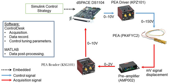
Figure 1.
Hardware–software configuration designed for the experiments.
2.2. Hysteresis and Reference Design
The typical profiles of references used in PEA guidance are triangular and sine waves [77]. Mainly, the hysteresis is better viewed with triangular waves, and this encourages another challenge for the control designer: these are complex signals with high-frequency harmonics and sharpened slope changes [78]. The selected amplitude was 140 V in order to avoid unnecessary saturations in the actuation signal and with a period of 4 s.
Figure 2 is a representation of the hysteresis acquired during the experiments in this investigation. In this case, 8 s of data were saved, which implies there are 2 cycles of the mentioned triangular signal. At the beginning, in point (a), known as the initial point, the PEA was calibrated at zero input voltage and displacement (these are capabilities that the KPZ101 and KSG101 provide). As the voltage was increased, the displacement did the same, which produced the curve C1 (named as the first ascending curve) until point (b). The latter, known as the upper converging point, is the point at which the maximum displacement (due to the 140 V) is reached. Thereafter, the voltage began to decrease as a consequence of the negative slope, and the curve C2 was generated. The latter ended in point (c), established as the lower converging point. It should be noticed that point (c) is different from (a). The second cycle begins from (c) and drew the curve C3 when the voltage increased and the displacement was acquired. The data converges at point (b) when the maximum voltage is reached again. The final voltage drop generates curve C4, which overlaps with the previous C2, and the same situation happens at the lower converging point where (c) is equal to (d).
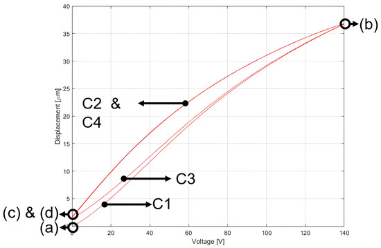
Figure 2.
PEA hysteresis graph acquired from experiments.
From the previous description and Figure 2, further details can be highlighted: (1) curve C1 was generated for the first half period from an initial calibration, which means that this path is unique for the first time; (2) the following cycles recurred between C2 and C3, which implies that the hysteresis takes place in an unique path provided that the voltage, signal type and period are constant; (3) points (a) and (c) are drift apart as a consequence of the creep effect [79]; (4) the hysteresis of the PEA used is asymmetric, which is a complex challenge in the design of advanced controllers.
On the other hand, the dynamic model of the PEA with nonlinear hysteresis can be described as Equation (1) [40].
where m, b, k, x, d, , h, and P are, respectively, mass, damping constant, stiffness, position, piezoelectric coefficient, input voltage, hysteresis, and general perturbations or unmodeled dynamics. The term represents the hysteresis that depends on the position.
2.3. Artificial Neural Network
The state-of-the-art reviews on hysteresis models in the introduction showed that these have certain limitations in modeling the real phenomenon. Even in some cases, realistic models may induce complex calculations that can increase the computational requirement. Thus, an ANN can be used to compensate for the hysteresis effect and reduce the computational cost, simplifying the system’s control. These are well known for their capabilities of compensation as black box models [80].
An ANN is described by four main features: its topology, training method, association type between input/output data, and information presentation [81]. In this case, a time delay neural network (TDNN) was used as it is known for its assets in system identification for time series [82]. As with any ANN, a TDNN has complex relationships that consist of processing units (known as “neurons”), which are linked with weights to other units to develop a network; but, in this case, the feature that distinguishes the structure from the others is that the input is weighted by delays, thus generating a finite dynamic response from input data series based on its previous history [83].
It has also been considered to use a Layer Recurrent Neural Network (LRNN) network, which shows similar characteristics. However, in TDNN time, aspect is only inserted through its inputs, unlike LSTM, which also needs the predicted future value as input. This characteristic makes TDNN less robust than LSTM for predicting values but requires less processing and is easier to train, which is in line with the idea of its implementation in a real environment with less powerful hardware than dSPACE.
The structure is resumed in Figure 3 where the inputs are delayed in n orders at the input layer. These are weighted in the hidden layer with k neurons plus biases, which are injected in a tansig activation function, known for its nonlinearity and robustness against noises [84]. The output r(t) from the hidden layer is fed into the output layer with a similar mechanism as the previous step but with a different activation function, like purelin. The latter is a common nonlinear function used in output layers of data series prediction models in ANNs [85].
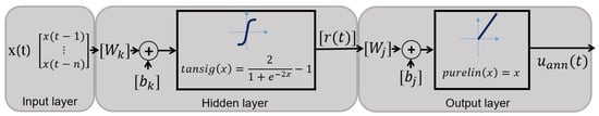
Figure 3.
Time-delay artificial neural network structure.
3. Control Strategies Design
The main experimental objective was to track a reference in contrast to four controllers: SMC, TA, STA, and PCL. The performance of each controller will be analyzed in terms of robustness and precision in graphics and numerical results. Hence, for further calculations, the error e is defined as in Equation (2), which is the difference between the measured position X and the given reference .
The general command expression of each control, according to the design proceedings of SMCs, is a split of two terms as shown in Equation (3): equivalent and switching (). Though the first one mentioned is usually achieved using a mathematical model of the system, an ANN was used in this case (). This is mainly because of the issues mentioned in Section 1 about hysteresis models. On the other hand, the switching term ensures the robustness of the scheme by means of the sliding behavior [86].
In order to provide a better understanding of the control strategy, Figure 4 is presented below.
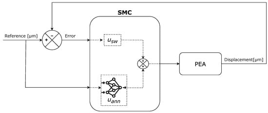
Figure 4.
Control strategy block diagram.
3.1. Conventional Sliding Mode Control
The first step in the design of an SMC is the choice of a suitable surface. In this sense, the guideline was followed through the criterion of Slotine et al. [87] that is expressed in Equation (4). The latter has the terms r and that are, respectively, the relative degree of the system and a positive constant.
Based on previous works [75], the relative degree from the system is 2. Therefore, the chosen sliding surface is as Equation (5) shows. This surface is also common for all the analyzed controllers in the following subsections.
The control law of the proposed controllers is established by a neural compensation to reach the sliding surface rather than an equivalent term that comes from a mathematical model, as it was explained in the introduction of this manuscript. Thus, the expression of the control signal for the conventional SMC is defined in Equation (6), where is the neural compensation (that will be explained in further sections) and is the switching term that provides robustness to the system. As in this case, the conventional SMC is being highlighted, the expression of is defined in Equation (7). The choice of should be positive, but what should be taken into account is that the bigger it gets, the higher the generated oscillations become [88].
Based on the former explanation, a formal stability proof has been performed using the system and the SMC algorithm. Considering previous Equation (1), the compensation term of the neural network of the Equation (6) can be considered, following the next Equation (8), as a superposition of a linear term (without perturbations or hysteresis, detailed in Equation (9)) named as and another which contemplates the nonlinearities that is defined as , which express the difference between the value of the ANN and the PEA physical model.
Hence, if the error is defined as in Equation (2), a system based on this variable is gathered in Equation (10). Also, it is considered that the ANN has an uncertainty in the fitting capabilities, for which reason it is defined as an approximation error .
In order to study the stability, the candidate Lyapunov function (based on the sliding surface S) proposed a quadratic Equation (11) and its derivative Equation (12), following the classical Lyapunov stability theory [87].
The previously defined surface in Equation (4) can be derivated and combined with the error second derivative from Equation (10). Therefore, through replacement, the first derivative of the Lyapunov function results in Equation (13):
where
For practical purposes, the term must tend toward a constant value since the error is expected to be small over time, and the perturbations with the neural network approximation will be finite and generally constant. Therefore, an upper and lower bound can be established based on the absolute value of a constant G such that [89]. Hence, with this assumption, Equation (15) is generated with the condition of stability according to Lyapunov’s theorem.
Hence, the previous expression can be achieved provided that , which will allow the second negative term to govern the stability condition of Lyapunov.
3.2. Twisting Algorithm
Similarly to the previously presented technique, the surface will be the same, but the control switching term is different as Equation (16) shows where the condition of the gains is that both are positive and [90].
In this case, a stability proof is fairly complex since conventional Lyapunov functions are not suitable for the analyzed system. Additionally, alternative proposals might result in a non-asymptotic stability (even using Lasalle’s theorem). Thus, the Lyapunov candidate function for this algorithm is meant to be Equation (17), the development of which can be found in the work of Santiesteban et al. [91].
3.3. Super-Twisting Algorithm
STA has been designed to reduce the chattering that TA produced as a first generation algorithm. Thus, the expression in this case corresponds with the one from Equation (18) that helps to provide a continuous control signal [92]. In this formula, the necessary conditions are that the constants K4 and K5 should be positive design parameters which will be gathered through minimization of the IAE. Additional details about the Lyapunov demonstration can be found in previous research from the authors [75].
3.4. Prescribed Convergence Law
PCL is a second-order SMC that ensures the surface and its derivatives (full dynamical collapse) will be null along the time and, therefore, the errors will converge to zero [93]. The minimum conditions that guarantee this statement are when and are positive numbers, whereas more related stability conditions can be found in the works from [94,95].
To summarize, the described four controllers with their key features are shown in the next Table 2.
Table 2.
Resume of the controllers and their key feature.
4. Results
4.1. Performance Metrics
The determination of the best performance was not only concluded on graph analysis but also under numerical reasoning. For this case, since the goal is to follow a reference, error-based metrics were taken into account. In real time, the calculation of the integral of the absolute error (IAE) was performed to achieve suitable control parameters based on the minimization of this metric Additional parameters that were calculated after the collection of the data were the root mean squared error (RMSE) and relative root mean squared error (RRMSE), which are also commonly used in tracking problems [96]. The three previously described tools are explained in Equation (21) where is the sampling time (which has been configured as 1 kHz), N points gathered for calculation and is the i-th trajectory point.
An additional parameter that will be introduced in this research is the duration of the computing unit of each controller. This has been performed through instructions “RTLIB_TIC_START()” and “RTLIB_TIC_READ()” from the capabilities of the dSPACE language library. These will provide the information of execution time measurement from the controller block.
4.2. Neural Network Training Results
The described TDNN was offline trained with data from triangular waves with an amplitude of 140 V and 4 s of period. Since the acquired data were the PEA displacement, this was used as an input in the ANN because an inverse model was needed in order to generate a compensation voltage.
In Table 3 the training parameters of the TDNN are presented. For the training algorithm, several were tested, and Levenberg–Marquadt (LM) provided the best results in terms of fitting and mean-squared error. This algorithm is able to solve nonlinear least squares for fitting problems with gradient-descent and Gauss-Newton methods [97].
Table 3.
TDNN training parameters.
In order to obtain the 10,000 Data points, the mentioned triangular waves with an amplitude of 140 V and 4 s of period were recorded along 10 s with a sampling time of 1 kHz. This allowed sufficient data that were split in typical ranges such as 70/15/15 for training, validation, and test sets, respectively [98].
It should be mentioned that the delay order chosen for the TDNN was obtained based on the optimization procedure by means of simulations, and it was determined to be 5. Moreover, for the training procedure, a last generation Dell Precision 3640 was employed in parallel configuration with 7 cores requiring 16.5 h to complete the training.
Figure 5 shows a test made in which the experimental results were contrasted against the output of the trained TDNN during a period of 4 s. The objective of this attempt was to evaluate the performance of the ANN as an inverse hysteresis model for the proposed controllers. Therefore, Figure 5a shows an error that averages around 0 V in the ascending curve until the first slope changes at 2 s. Surrounding this point, the error increases its amplitude to around 0.6 V, which means less than 1% of difference to the expected value, which is a satisfactory range.
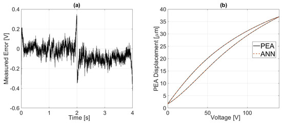
Figure 5.
Fitting capability of the configured ANN: (a) fitting error; (b) hysteresis contrasted with the experimental data.
4.3. Control Implementation Results
All four described strategies had been embedded in the dSPACE platform, which provided information that was processed for graphical and numerical analysis. The following figures present the collected information achieved during the tracking of a triangular signal with an amplitude of 140 V and a period of 2 s. All controllers showed different performance and control signals, which are both analyzed as follows. It should be noted that time delays introduced by sensors, actuators, computational delays, etc., are not considered in this test.
The gains of each controller that were gathered by means of minimization of IAE are shown in Table 4.
Table 4.
Achieved gains through minimization of IAE for each controller.
Figure 6 demonstrates the acquired error during 8s, which is two triangular wave cycles. This reference was selected since it allows us to observe the performance of the controllers in the peaks of the hysteresis curve where the ANN showed the worst errors. Graphically, the main spots to be analyzed are the slope changes (2 s, 4 s, and 6 s), and a general conclusion can be achieved through numerical tools to grant a better verdict. Figure 6a displays the error in the first slope switch from rising to decreasing voltage in a short time range. It can be seen that all the controllers behave similarly in the change since an overshoot is generated. In this sense, the strategy that provided the higher overshoot has been TA (0.17 V) whereas the lowest one was STA (0.12 V), which also gave the best settling time (near 0.018 s). It can also be seen that after 2 s, TA showed more variation in the amplitude than the conventional SMC, expected to be the algorithm with more chattering.
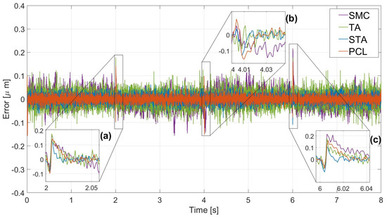
Figure 6.
Tracking error comparison of the embedded controllers: (a) first slope change; (b) second slope change; (c) third slope change.
At the lower converging point in 4 s (shown in Figure 6b), the performance of the controllers is rather different, though the TA still has enough variation. The PCL algorithm seems to provide the highest undershoot because the amplitude was around 0.25 V in contrast to the 0.08 V from STA, which specified the lowest value. The settling time has also achieved the best value with STA, which has been around 0.016 s.
Despite that it was expected a similar behavior at 6 s, SMC and TA behaved differently. Figure 6c sights a higher error value in the generated amplitude of SMC with a slower settling time in comparison to the other controllers. Additionally, it also shows higher chattering along the time than TA until 6.03 s, which is when the situation changes and TA generates even more.
Numerical results were achieved based on the data gathered from Figure 6, which are mirrored in Table 5 by tools explained in Section 4.1. The values of IAE and RMSE had been referenced to the SMC, which showed the highest in both metrics. TA exhibited a similar value in both metrics with a difference below 10%. Nevertheless, STA boosted the difference as it reached almost 50% of dissimilarity with SMC. Thus, the PCL algorithm prevails over the rest of the options as it showed a significant enhancement of above 55% in IAE and RMSE. The RRMSE expressed the same trend since the difference between SMC and PCL was progressive: the PCL showed half of the value of the SMC.
Table 5.
Metrics comparison for the tested controllers.
Figure 7 represents the acquired control signal, which was produced by the algorithms along with the error compensation that has been previously analyzed. Although saturation can damage the actuator, which was unseen during experiments, several zoomed windows are provided to accomplish a better analysis in each part. For instance, Figure 7a shows an expected scenario during the beginning where the TA generated a considerable variable signal in contrast to the other algorithms. Actually, it can be seen that PCL was able to provide a softer response indeed; these phenomena can be seen in Figure 7e. In Figure 7b,d, otherwise, a sudden change in control signal can be seen. This happens because the controller needs to compensate for the hysteresis effect. If the displacement of the PEA does not reach the maximum, where the two curves of the hysteresis converge, the system goes from one curve to another (from C3 to C4 of Figure 2 or vice versa), immediately forcing the controller to compensate that change.
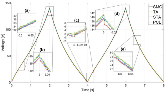
Figure 7.
Control signal comparison of the embedded controllers: (a) first interest point; (b) first slope change; (c) second slope change; (d) third slope change; Fifth interest point (e).
Later, in Figure 7c, the previous trend is still the same as the TA provided more chattering than other options. It is also possible to see that all the controllers made a necessary sharp switch due to the slope change, but PCL had the lowest amplitude change. Nevertheless, in Figure 7c, the switch was softer, with slight overshoots in all the frameworks.
Lastly, Figure 8 provides the required computational time with its mean and standard deviation for each control strategy. The computational time is the one needed to execute once the control algorithm, which differs from the sample time of 1 ms (1 kHz). These data are an important feature because it provides an idea to a designer about the choice required for a hardware control board. At first, it can be seen that the SMC requires the lowest time (which means 1.07 µs) due to its simplicity. TA uses a derivative term, which makes sense as the value increment is 1.42 µs, which is a 32% increase in comparison to SMC. However, TA provided a lower standard deviation in comparison. On the other hand, STA shows an almost similar computational time to TA since its value is 1.53 µs, which is 42% more than SMC. Finally, PCL gave the highest value, which has been almost 2 µs with the highest standard deviation in comparison with all the other algorithms. This implies that PCL has 86% higher time consumption than conventional SMC. This leads to the conclusion, taking into account the values obtained in the previous Table 5, that the better the performance of the controller, the higher the computational cost.
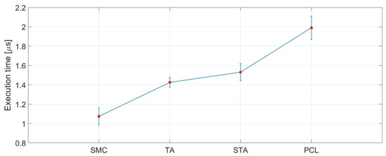
Figure 8.
Computational time comparison of the embedded controllers.
Thus, it can be concluded that, in general terms, there is an indirect relationship between execution time and performance: the longer the computation time (as in the case of PCL), the higher the computational cost, but also the better the tracking performance and the controller’s ability to handle complex scenarios. However, the STA controller, despite having a moderate execution time, has proven to be the most robust against disturbances and system uncertainties. On the other hand, TA, whose performance is similar to that of SMC, shows a slight increase in execution time without a significant improvement in control performance.
In terms of application, SMC may be suitable for embedded systems with limited resources or simple control tasks. TA and STA offer intermediate solutions, ideal for environments requiring a balance between efficiency and performance—although TA’s tracking performance is comparable to that of conventional SMC, making STA the preferable choice in such scenarios. Finally, PCL appears to be the best option for critical systems where high performance is essential and more powerful hardware is available.
5. Conclusions
In this research, four sliding controllers with a neural combination for tracking reference following were analyzed and embedded in a PEA. Traditional methods like conventional SMC and TA were contrasted with the advanced ones such as STA or PCL; the outcomes were correlated to determine the best performance of each in a complex reference to be followed, including a triangular wave.
An experimental setup was built using a commercial PEA (PK4FYC2) and Thorlabs peripherals, which were interfaced with a DS1104 board. Hysteresis properties were characterized by comparing the first and subsequent cycle curves, thus highlighting the creep effect. Using these data, an ANN was trained to replace classical approaches, addressing computational load and parameter identification issues. The resulting TDNN showed good fitting performance with the PEA hysteresis, making it suitable for integration into a control system.
Results showed that STA developed the best response due to the lowest under-/overshoot and settling time. Therefore, the STA combined with an ANN is established as the most robustly tested algorithm, as observed graphically. Furthermore, in numerical metrics, PCL achieved better performance over the rest of the algorithm. Behind the PCL, STA also provided a suitable demeanour, which implies that it has not only delivered the most robust development but also generated one of the best numerical results.
The consumption time of each algorithm was also analyzed. Overall, the study reveals a trade-off between execution time and control performance: more complex controllers like PCL offer superior tracking and adaptability at the cost of higher computational demands. Among the alternatives, STA stands out for its robustness and balanced execution time, making it a strong candidate for systems facing uncertainties. Despite being slightly more demanding than SMC, TA does not provide notable performance gains. In terms of applicability, SMC suits simple or resource-constrained systems, STA is ideal when robustness is key, and PCL is recommended for high-performance, computation-rich environments.
In future research, the expected studies will first focus on the investigation of various ANNs, which can allow for a better hysteresis reflection. Complex architectures like long short-term memory or gate recurrent units can be evaluated in sliding controllers. In terms of control approaches, an evaluation of other sliding controllers, such as global and terminal structures, can be embedded in the real-time control board.
Author Contributions
Conceptualization, C.N. and O.B.; methodology, C.N. and O.B.; software, C.N.; validation, O.B.; formal analysis, C.N. and O.B.; investigation, C.N.; resources, O.B.; data curation, C.N.; writing—original draft preparation, C.N.; writing—review and editing, J.U., O.B., I.C., E.A. and A.d.R.; visualization, J.U. and E.A.; supervision, O.B. and I.C.; project administration, O.B. and I.C. All authors have read and agreed to the published version of the manuscript.
Funding
This research received no external funding.
Data Availability Statement
The original contributions presented in this study are included in the article. Further inquiries can be directed to the corresponding authors.
Acknowledgments
The authors wish to express their gratitude to the Basque Government, through the project NEWHEGAZ (ELKARTEK KK-2025/00074), to the UPV/EHU, through the project GIU23/002, and to the MobilityLab Foundation (CONV23/14, CONV23/12) for supporting this work.
Conflicts of Interest
The authors declare no conflicts of interest.
References
- Esashi, M. MEMS development focusing on collaboration using common facilities: A retrospective view and future directions. Microsyst. Nanoeng. 2021, 7, 60. [Google Scholar] [CrossRef] [PubMed]
- Zou, H.; Chen, H.; Zhu, X. Piezoelectric energy harvesting from vibrations induced by jet-resonator system. Mechatronics 2015, 26, 29–35. [Google Scholar] [CrossRef]
- Goyal, J.; Khandnor, P.; Aseri, T.C. Classification, Prediction, and Monitoring of Parkinson’s disease using Computer Assisted Technologies: A Comparative Analysis. Eng. Appl. Artif. Intell. 2020, 96, 103955. [Google Scholar] [CrossRef]
- McClintock, H.; Temel, F.Z.; Doshi, N.; sung Koh, J.; Wood, R.J. The milliDelta: A high-bandwidth, high-precision, millimeter-scale Delta robot. Sci. Robot. 2018, 3, eaar3018. [Google Scholar] [CrossRef]
- Son, N.N.; Van Kien, C.; Anh, H.P.H. Parameters identification of Bouc–Wen hysteresis model for piezoelectric actuators using hybrid adaptive differential evolution and Jaya algorithm. Eng. Appl. Artif. Intell. 2020, 87, 103317. [Google Scholar] [CrossRef]
- De Jong, M.C.; Kosaraju, K.C.; Scherpen, J.M. On control of voltage-actuated piezoelectric beam: A Krasovskii passivity-based approach. Eur. J. Control 2023, 69, 100724. [Google Scholar] [CrossRef]
- Liu, R.; Wen, Z.; Cao, T.; Lu, C.; Wang, B.; Wu, D.; Li, X. A precision positioning rotary stage driven by multilayer piezoelectric stacks. Precis. Eng. 2022, 76, 226–236. [Google Scholar] [CrossRef]
- Judy, J.W. Microactuators. In MEMS: A Practical Guide to Design, Analysis, and Applications; Springer: Berlin/Heidelberg, Germany, 2006; Chapter 14; pp. 751–803. [Google Scholar] [CrossRef]
- Damjanovic, D.; Demartin, M. Contribution of the irreversible displacement of domain walls to the piezoelectric effect in barium titanate and lead zirconate titanate ceramics. J. Phys. Condens. Matter 1997, 9, 4943–4953. [Google Scholar] [CrossRef]
- Fancher, C.; Brewer, S.; Chung, C.; Röhrig, S.; Rojac, T.; Esteves, G.; Deluca, M.; Bassiri-Gharb, N.; Jones, J. The contribution of 180° domain wall motion to dielectric properties quantified from in situ X-ray diffraction. Acta Mater. 2017, 126, 36–43. [Google Scholar] [CrossRef]
- Zhong, J.; Nishida, R.; Shinshi, T. A digital charge control strategy for reducing the hysteresis in piezoelectric actuators: Analysis, design, and implementation. Precis. Eng. 2021, 67, 370–382. [Google Scholar] [CrossRef]
- Zheng, T.; Wu, J.; Xiao, D.; Zhu, J. Recent development in lead-free perovskite piezoelectric bulk materials. Prog. Mater. Sci. 2018, 98, 552–624. [Google Scholar] [CrossRef]
- Damjanovic, D. Hysteresis in piezoelectric and ferroelectric materials. In The Science of Hysteresis; Academic Press: Cambridge, MA, USA, 2006; Chapter 4; pp. 338–452. [Google Scholar] [CrossRef]
- Han, W.; Shao, S.; Zhang, S.; Tian, Z.; Xu, M. Design and modeling of decoupled miniature fast steering mirror with ultrahigh precision. Mech. Syst. Signal Process. 2022, 167, 108521. [Google Scholar] [CrossRef]
- Wang, S.; Chen, Z.; Liu, X.; Jiao, Y. Feedforward Feedback Linearization Linear Quadratic Gaussian With Loop Transfer Recovery Control of Piezoelectric Actuator in Active Vibration Isolation System. J. Vib. Acoust. 2018, 140, 041009. [Google Scholar] [CrossRef]
- Yeh, Y.L. Output Feedback Tracking Sliding Mode Control for Systems with State- and Input-Dependent Disturbances. Actuators 2021, 10, 117. [Google Scholar] [CrossRef]
- Vestroni, F.; Casini, P. Nonlinear Dynamics and Phenomena in Oscillators with Hysteresis. In Modern Trends in Structural and Solid Mechanics 2; John Wiley & Sons, Ltd.: New York, NY, USA, 2021; Chapter 8; pp. 185–202. [Google Scholar] [CrossRef]
- Iqbal, J.; Ullah, M.; Khan, S.G.; Khelifa, B.; Ćuković, S. Nonlinear control systems - A brief overview of historical and recent advances. Nonlinear Eng. 2017, 6, 301–312. [Google Scholar] [CrossRef]
- Dumitrescu, C.; Ciotirnae, P.; Vizitiu, C. Fuzzy Logic for Intelligent Control System Using Soft Computing Applications. Sensors 2021, 21, 2617. [Google Scholar] [CrossRef]
- Dawei, M.; Yu, Z.; Meilan, Z.; Risha, N. Intelligent fuzzy energy management research for a uniaxial parallel hybrid electric vehicle. Comput. Electr. Eng. 2017, 58, 447–464. [Google Scholar] [CrossRef]
- Roselyn, J.P.; Devaraj, D.; Venkatesan, R.; Raj, A.; Chandran, C.P. Development and real time implementation of intelligent holistic power control for stand alone solar photovoltaic generation system. Comput. Electr. Eng. 2021, 96, 107519. [Google Scholar] [CrossRef]
- Chiu, C.H.; Hung, Y.T. One wheel vehicle real world control based on interval type 2 fuzzy controller. Mechatronics 2020, 70, 102387. [Google Scholar] [CrossRef]
- Zhang, X.; Chen, X.; Zhu, G.; Su, C.Y. Output Feedback Adaptive Motion Control and Its Experimental Verification for Time-Delay Nonlinear Systems With Asymmetric Hysteresis. IEEE Trans. Ind. Electron. 2020, 67, 6824–6834. [Google Scholar] [CrossRef]
- Luo, Y.; Zhang, X.; Zhang, Y.; Qu, Y.; Xu, M.; Fu, K.; Ye, L. Active vibration control of a hoop truss structure with piezoelectric bending actuators based on a fuzzy logic algorithm. Smart Mater. Struct. 2018, 27, 085030. [Google Scholar] [CrossRef]
- Schwenzer, M.; Muzaffer, A.; Bergs, T.; Dirk, A. Review on model predictive control: An engineering perspective. Int. J. Adv. Manuf. Technol. 2021, 117, 1327–1349. [Google Scholar] [CrossRef]
- Du, Z.; Zhou, C.; Cao, Z.; Wang, S.; Cheng, L.; Tan, M. A neural network-based model predictive controller for displacement tracking of piezoelectric actuator with feedback delays. Int. J. Adv. Robot. Syst. 2021, 18, 17298814211057698. [Google Scholar] [CrossRef]
- Chanal, P.M.; Kakkasageri, M.S.; Manvi, S.K.S. Chapter 7 - Security and privacy in the internet of things: Computational intelligent techniques-based approaches. In Recent Trends in Computational Intelligence Enabled Research; Bhattacharyya, S., Dutta, P., Samanta, D., Mukherjee, A., Pan, I., Eds.; Academic Press: Cambridge, MA, USA, 2021; pp. 111–127. [Google Scholar] [CrossRef]
- Eminoǧlu, I.; Altaş, I.H. The effects of the number of rules on the output of a fuzzy logic controller employed to a PM d.c. motor. Comput. Electr. Eng. 1998, 24, 245–261. [Google Scholar] [CrossRef]
- Nagi, F.; Perumal, L. Optimization of fuzzy controller for minimum time response. Mechatronics 2009, 19, 325–333. [Google Scholar] [CrossRef]
- Wang, J.; Shao, C.; Chen, Y.Q. Fractional order sliding mode control via disturbance observer for a class of fractional order systems with mismatched disturbance. Mechatronics 2018, 53, 8–19. [Google Scholar] [CrossRef]
- Özbek, N.S. Design and real-time implementation of a robust fractional second-order sliding mode control for an electromechanical system comprising uncertainties and disturbances. Eng. Sci. Technol. Int. J. 2022, 35, 101212. [Google Scholar] [CrossRef]
- Jena, N.K.; Sahoo, S.; Sahu, B.K.; Nayak, J.R.; Mohanty, K.B. Fuzzy adaptive selfish herd optimization based optimal sliding mode controller for frequency stability enhancement of a microgrid. Eng. Sci. Technol. Int. J. 2022, 33, 101071. [Google Scholar] [CrossRef]
- Kwan, C.; Dawson, D.M.; Lewis, F.L. Robust Adaptive Control of Robots Using Neural Network: Global Stability. Asian J. Control 2001, 3, 111–121. [Google Scholar] [CrossRef]
- Napole, C.; Derbeli, M.; Barambones, O. A global integral terminal sliding mode control based on a novel reaching law for a proton exchange membrane fuel cell system. Appl. Energy 2021, 301, 117473. [Google Scholar] [CrossRef]
- Liang, C.; Wang, F.; Shi, B.; Huo, Z.; Zhou, K.; Tian, Y.; Zhang, D. Design and control of a novel asymmetrical piezoelectric actuated microgripper for micromanipulation. Sens. Actuators A Phys. 2018, 269, 227–237. [Google Scholar] [CrossRef]
- Lau, J.Y.; Liang, W.; Liaw, H.C.; Tan, K.K. Sliding Mode Disturbance Observer-based Motion Control for a Piezoelectric Actuator-based Surgical Device. Asian J. Control 2018, 20, 1194–1203. [Google Scholar] [CrossRef]
- Liaw, H.C.; Shirinzadeh, B.; Smith, J. Enhanced sliding mode motion tracking control of piezoelectric actuators. Sens. Actuators A Phys. 2007, 138, 194–202. [Google Scholar] [CrossRef]
- Chang, K.M.; Chen, J.M.; Liu, Y.T. Nonlinear sliding mode control for piezoelectric tool holder with bellows-type hydraulic displacement amplification mechanism. Sens. Actuators A Phys. 2023, 361, 114543. [Google Scholar] [CrossRef]
- Zare, M.; Pazooki, F.; Haghighi, S.E. Hybrid controller of Lyapunov-based and nonlinear fuzzy-sliding mode for a quadrotor slung load system. Eng. Sci. Technol. Int. J. 2022, 29, 101038. [Google Scholar] [CrossRef]
- Chouza, A.; Barambones, O.; Calvo, I.; Velasco, J. Sliding Mode-Based Robust Control for Piezoelectric Actuators with Inverse Dynamics Estimation. Energies 2019, 12, 943. [Google Scholar] [CrossRef]
- Xu, R.; Zhou, M. Sliding mode control with sigmoid function for the motion tracking control of the piezo-actuated stages. Electron. Lett. 2017, 53, 75–77. [Google Scholar] [CrossRef]
- Shtessel, Y.B.; Shkolnikov, I.A.; Brown, M.D. An Asymptotic Second-Order Smooth Sliding Mode Control. Asian J. Control 2003, 5, 498–504. [Google Scholar] [CrossRef]
- Wang, X.; Zhang, Y.; Gao, P. Design and Analysis of Second-Order Sliding Mode Controller for Active Magnetic Bearing. Energies 2020, 13, 5965. [Google Scholar] [CrossRef]
- Utkin, V.; Poznyak, A.; Orlov, Y.; Polyakov, A. Conventional and high order sliding mode control. J. Frankl. Inst. 2020, 357, 10244–10261. [Google Scholar] [CrossRef]
- Fridman, L.; Moreno, J.A.; Bandyopadhyay, B.; Kamal, S.; Chalanga, A. Continuous Nested Algorithms: The Fifth Generation of Sliding Mode Controllers. In Recent Advances in Sliding Modes: From Control to Intelligent Mechatronics; Springer International Publishing: Berlin/Heidelberg, Germany, 2015; Chapter 2; pp. 5–35. [Google Scholar] [CrossRef]
- Deepika, D.; Kaur, S.; Narayan, S. Integral terminal sliding mode control unified with UDE for output constrained tracking of mismatched uncertain non-linear systems. ISA Trans. 2020, 101, 1–9. [Google Scholar] [CrossRef]
- Wang, G.; Wang, B.; Zhang, C. Fixed-Time Third-Order Super-Twisting-like Sliding Mode Motion Control for Piezoelectric Nanopositioning Stage. Mathematics 2021, 9, 1770. [Google Scholar] [CrossRef]
- Shah, D.; Shah, A.; Mehta, A. Higher order networked sliding mode controller for heat exchanger connected via data communication network. Eur. J. Control 2021, 58, 301–314. [Google Scholar] [CrossRef]
- Seyedtabaii, S. Modified adaptive second order sliding mode control: Perturbed system response robustness. Comput. Electr. Eng. 2020, 81, 106536. [Google Scholar] [CrossRef]
- Li, C.; Wang, Y.; Liu, L. Path Following Control of Ship Based on Time-Varying Threshold Prescribed Convergence Law Sliding Mode. In Proceedings of the 2018 37th Chinese Control Conference (CCC), Wuhan, China, 25–27 July 2018; pp. 525–530. [Google Scholar] [CrossRef]
- Xu, Q. Continuous Integral Terminal Third-Order Sliding Mode Motion Control for Piezoelectric Nanopositioning System. IEEE/ASME Trans. Mechatronics 2017, 22, 1828–1838. [Google Scholar] [CrossRef]
- Napole, C.; Barambones, O.; Calvo, I.; Derbeli, M.; Silaa, M.; Velasco, J. Advances in Tracking Control for Piezoelectric Actuators Using Fuzzy Logic and Hammerstein-Wiener Compensation. Mathematics 2020, 8, 2071. [Google Scholar] [CrossRef]
- Armin, M.; Roy, P.N.; Das, S.K. A Survey on Modelling and Compensation for Hysteresis in High Speed Nanopositioning of AFMs: Observation and Future Recommendation. Int. J. Autom. Comput. 2020, 17, 479. [Google Scholar] [CrossRef]
- Shi, P. One-dimensional magneto-mechanical model for anhysteretic magnetization and magnetostriction in ferromagnetic materials. J. Magn. Magn. Mater. 2021, 537, 168212. [Google Scholar] [CrossRef]
- Thiele, G.; Fey, A.; Sommer, D.; Kruger, J. System identification of a hysteresis-controlled pump system using SINDy. In Proceedings of the 2020 24th International Conference on System Theory, Control and Computing (ICSTCC), Sinaia, Romania, 8–10 October 2020; pp. 457–464. [Google Scholar] [CrossRef]
- Semenov, M.; Reshetova, O.; Borzunov, S.; Meleshenko, P. Self-oscillations in a system with hysteresis: The small parameter approach. Eur. Phys. J. Spec. Top. 2021, 230, 3565–3571. [Google Scholar] [CrossRef]
- Li, Z.; Shan, J.; Gabbert, U. A Direct Inverse Model for Hysteresis Compensation. IEEE Trans. Ind. Electron. 2021, 68, 4173–4181. [Google Scholar] [CrossRef]
- Al Janaideh, M.; Davino, D.; Krejčí, P.; Visone, C. Comparison of Prandtl–Ishlinskiı˘ and Preisach modeling for smart devices applications. Phys. B Condens. Matter 2016, 486, 155–159. [Google Scholar] [CrossRef]
- Zheng, L.; Weijie, D. Position and force self-sensing piezoelectric valve with hysteresis compensation. J. Intell. Mater. Syst. Struct. 2021, 33, 1045389X2110116. [Google Scholar] [CrossRef]
- Lin, J.; Chiang, M. Tracking Control of a Magnetic Shape Memory Actuator Using an Inverse Preisach Model with Modified Fuzzy Sliding Mode Control. Sensors 2016, 16, 1368. [Google Scholar] [CrossRef] [PubMed]
- Riccardo, S.; Riganti-Fulginei, F.; Laudani, A.; Quandam, S. Algorithms to reduce the computational cost of vector Preisach model in view of Finite Element analysis. J. Magn. Magn. Mater. 2022, 546, 168876. [Google Scholar] [CrossRef]
- Shao, M.; Wang, Y.; Gao, Z.; Zhu, X. Discrete-time rate-dependent hysteresis modeling and parameter identification of piezoelectric actuators. Trans. Inst. Meas. Control 2022, 44, 10. [Google Scholar] [CrossRef]
- Li, Z.; Li, J.; Weng, T.; Zheng, Z. Adaptive Backstepping Time Delay Control for Precision Positioning Stage with Unknown Hysteresis. Mathematics 2024, 12, 1197. [Google Scholar] [CrossRef]
- Zhu, X.; Lu, X. Parametric Identification of Bouc-Wen Model and Its Application in Mild Steel Damper Modeling. Procedia Eng. 2011, 14, 318–324. [Google Scholar] [CrossRef]
- Salah, M.; Saleem, A. Hysteresis compensation-based robust output feedback control for long-stroke piezoelectric actuators at high frequency. Sens. Actuators A Phys. 2021, 319, 112542. [Google Scholar] [CrossRef]
- Sun, Y.; Ma, H.; Li, Y.; Liu, Z.; Xiong, Z. A Novel Rate-dependent Direct Inverse Preisach Model With Input Iteration for Hysteresis Compensation of Piezoelectric Actuators. Int. J. Control. Autom. Syst. 2024, 22, 1277–1288. [Google Scholar] [CrossRef]
- Licciardi, S.; Ala, G.; Francomano, E.; Viola, F.; Giudice, M.L.; Salvini, A.; Sargeni, F.; Bertolini, V.; Schino, A.D.; Faba, A. Neural Network Architectures and Magnetic Hysteresis: Overview and Comparisons. Mathematics 2024, 12, 3363. [Google Scholar] [CrossRef]
- Lin, F.J.; Lee, S.Y.; Chou, P.H. Intelligent Integral Backstepping Sliding-mode Control Using Recurrent Neural Network For Piezo-flexural Nanopositioning Stage. Asian J. Control 2016, 18, 456–472. [Google Scholar] [CrossRef]
- Meng, D.; Xia, P.; Lang, K.; Smith, E.C.; Rahn, C.D. Neural Network Based Hysteresis Compensation of Piezoelectric Stack Actuator Driven Active Control of Helicopter Vibration. Sens. Actuators A Phys. 2020, 302, 111809. [Google Scholar] [CrossRef]
- Li, W.; Chen, X. Compensation of hysteresis in piezoelectric actuators without dynamics modeling. Sens. Actuators A Phys. 2013, 199, 89–97. [Google Scholar] [CrossRef]
- Wang, Y.F.; Zhou, M.L.; Shen, C.L.; Cao, W.J.; Huang, X.L. Time delay recursive neural network-based direct adaptive control for a piezo-actuated stage. Sci. China Technol. Sci. 2023, 66, 1397–1407. [Google Scholar] [CrossRef]
- Yan, G. Inverse neural networks modelling of a piezoelectric stage with dominant variable. J. Braz. Soc. Mech. Sci. Eng. 2021, 43, 387. [Google Scholar] [CrossRef]
- Artetxe, E.; Barambones, O.; Calvo, I.; del Rio, A.; Uralde, J. Combined Control for a Piezoelectric Actuator Using a Feed-Forward Neural Network and Feedback Integral Fast Terminal Sliding Mode Control. Micromachines 2024, 15, 757. [Google Scholar] [CrossRef]
- Tao, Y.D.; Li, H.X.; Zhu, L.M. Rate-dependent hysteresis modeling and compensation of piezoelectric actuators using Gaussian process. Sens. Actuators A Phys. 2019, 295, 357–365. [Google Scholar] [CrossRef]
- Napole, C.; Barambones, O.; Derbeli, M.; Calvo, I.; Silaa, M.Y.; Velasco, J. High-Performance Tracking for Piezoelectric Actuators Using Super-Twisting Algorithm Based on Artificial Neural Networks. Mathematics 2021, 9, 244. [Google Scholar] [CrossRef]
- Napole, C.; Barambones, O.; Derbeli, M.; Calvo, I. Advanced Trajectory Control for Piezoelectric Actuators Based on Robust Control Combined with Artificial Neural Networks. Appl. Sci. 2021, 11, 7390. [Google Scholar] [CrossRef]
- Xiong, R.; Liu, X.; Lai, Z. Modeling of Hysteresis in Piezoelectric Actuator Based on Segment Similarity. Micromachines 2015, 6, 1805–1824. [Google Scholar] [CrossRef]
- Qin, Y.; Duan, H. Single-Neuron Adaptive Hysteresis Compensation of Piezoelectric Actuator Based on Hebb Learning Rules. Micromachines 2020, 11, 84. [Google Scholar] [CrossRef] [PubMed]
- Tang, H.; Li, Y. Feedforward nonlinear PID control of a novel micromanipulator using Preisach hysteresis compensator. Robot. Comput.-Integr. Manuf. 2015, 34, 124–132. [Google Scholar] [CrossRef]
- Fu, J.; Yang, R.; Li, X.; Sun, X.; Li, Y.; Liu, Z.; Zhang, Y.; Sunden, B. Application of artificial neural network to forecast engine performance and emissions of a spark ignition engine. Appl. Therm. Eng. 2022, 201, 117749. [Google Scholar] [CrossRef]
- Marugán, A.P.; Márquez, F.P.G.; Perez, J.M.P.; Ruiz-Hernández, D. A survey of artificial neural network in wind energy systems. Appl. Energy 2018, 228, 1822–1836. [Google Scholar] [CrossRef]
- Drgoňa, J.; Picard, D.; Kvasnica, M.; Helsen, L. Approximate model predictive building control via machine learning. Appl. Energy 2018, 218, 199–216. [Google Scholar] [CrossRef]
- Khoshand, A. Application of artificial intelligence in groundwater ecosystem protection: A case study of Semnan/Sorkheh plain, Iran. Environ. Dev. Sustain. 2021, 23, 16617–16631. [Google Scholar] [CrossRef]
- Ghazvini, A.; Abdullah, S.N.H.S.; Kamrul Hasan, M.; Bin Kasim, D.Z.A. Crime Spatiotemporal Prediction With Fused Objective Function in Time Delay Neural Network. IEEE Access 2020, 8, 115167–115183. [Google Scholar] [CrossRef]
- Amani, P.; Vajravelu, K. Intelligent modeling of rheological and thermophysical properties of green covalently functionalized graphene nanofluids containing nanoplatelets. Int. J. Heat Mass Transf. 2018, 120, 95–105. [Google Scholar] [CrossRef]
- Eker, İ. Second-order sliding mode control with experimental application. ISA Trans. 2010, 49, 394–405. [Google Scholar] [CrossRef]
- Slotine, J.; Li, W. Sliding Surfaces. In Applied Nonlinear Control; Prentice Hall: Englewood Cliffs, NJ, USA, 1991; Chapter Sliding Control; pp. 278–279. [Google Scholar]
- Zhang, B.; Nie, K.; Chen, X.; Mao, Y. Development of Sliding Mode Controller Based on Internal Model Controller for Higher Precision Electro-Optical Tracking System. Actuators 2022, 11, 16. [Google Scholar] [CrossRef]
- Moreno, J.A.; Osorio, M. Strict Lyapunov Functions for the Super-Twisting Algorithm. IEEE Trans. Autom. Control 2012, 57, 1035–1040. [Google Scholar] [CrossRef]
- Shtessel, Y.; Edwards, C.; Fridman, L.; Levant, A. Second-Order Sliding Mode Controllers and Differenciators. In Sliding Mode Control and Observation; Springer: New York, NY, USA, 2014; Chapter 4; pp. 143–182. [Google Scholar] [CrossRef]
- Santiesteban, R.; Fridman, L.; Moreno, J. Finite-time convergence analysis for “Twisting” controller via a strict Lyapunov function. In Proceedings of the 2010 11th International Workshop on Variable Structure Systems (VSS), Mexico City, Mexico, 26–28 June 2010; pp. 1–6. [Google Scholar] [CrossRef]
- Moreno, J.; Ríos, H.; Ovalle, L.; Fridman, L. Multivariable Super-Twisting Algorithm for Systems with Uncertain Input Matrix and Perturbations. IEEE Trans. Autom. Control 2021, 67, 6716–6722. [Google Scholar] [CrossRef]
- Shtessel, Y.; Edwards, C.; Fridman, L.; Levant, A. Introduction: Intuitive Theory of Sliding Mode Control. In Sliding Mode Control and Observation; Springer: New York, NY, USA, 2014; Chapter 1; pp. 1–42. [Google Scholar] [CrossRef]
- Fridman, L.; Levant, A. Higher-Order Sliding Modes; CRC Press: Boca Raton, FL, USA, 2002; Volume 11, Chapter 3; pp. 53–101. [Google Scholar] [CrossRef]
- Shtessel, Y.B.; Ghanes, M.; Ashok, R.S. Hydrogen Fuel Cell and Ultracapacitor Based Electric Power System Sliding Mode Control: Electric Vehicle Application. Energies 2020, 13, 2798. [Google Scholar] [CrossRef]
- Wang, Y.; Zhang, Y.; Wu, J.; Huang, P.; Zhang, P. Tracking control of dielectric elastomer actuators for soft robots based on inverse dynamic compensation method. Inf. Sci. 2022, 583, 202–218. [Google Scholar] [CrossRef]
- Pachouly, J.; Ahirrao, S.; Kotecha, K.; Selvachandran, G.; Abraham, A. A systematic literature review on software defect prediction using artificial intelligence: Datasets, Data Validation Methods, Approaches, and Tools. Eng. Appl. Artif. Intell. 2022, 111, 104773. [Google Scholar] [CrossRef]
- Bilal, D.K.; Unel, M.; Tunc, L.T.; Gonul, B. Development of a vision based pose estimation system for robotic machining and improving its accuracy using LSTM neural networks and sparse regression. Robot. Comput.-Integr. Manuf. 2022, 74, 102262. [Google Scholar] [CrossRef]
Disclaimer/Publisher’s Note: The statements, opinions and data contained in all publications are solely those of the individual author(s) and contributor(s) and not of MDPI and/or the editor(s). MDPI and/or the editor(s) disclaim responsibility for any injury to people or property resulting from any ideas, methods, instructions or products referred to in the content. |
© 2025 by the authors. Licensee MDPI, Basel, Switzerland. This article is an open access article distributed under the terms and conditions of the Creative Commons Attribution (CC BY) license (https://creativecommons.org/licenses/by/4.0/).