Prediction of Water Quality in Agricultural Watersheds Based on VMD-GA-LSTM Model

Abstract

As agricultural non-point source pollution becomes increasingly severe and constitutes the primary source of water quality degradation, accurately predicting water quality in agricultural watersheds has become critical for environmental protection. In order to solve the nonlinear and non-stationary characteristics of water quality data, this paper proposes a combined model based on variational modal decomposition and genetic algorithm optimization of long short-term memory networks (VMD-GA-LSTM) for agricultural watershed water quality prediction. The VMD-GA-LSTM model utilizes the variational mode decomposition technique to decompose the time series data into multiple intrinsic mode functions and then uses the optimized LSTM network to predict each component to improve the accuracy of water quality prediction. The analysis of water quality data from the Baima River in China demonstrated that the VMD-GA-LSTM model significantly reduced prediction errors compared to other similar models. The VMD-GA-LSTM predictive model proposed in this paper effectively addresses the volatility characterizing water quality in agricultural watersheds, improves prediction accuracy, and it reveals valuable trends in water quality dynamics, providing practical solutions for sustainable agricultural practices and environmental governance.

1. Introduction

Water quality management in agricultural watersheds is pivotal to sustaining ecological integrity and human well-being globally. Agricultural activities, particularly fertilizer overuse and livestock waste runoff, are dominant contributors to aquatic pollution, releasing excess ammonia and nitrogen into water systems [1]. These pollutants cause eutrophication, toxic algal blooms, and biodiversity loss, damaging aquatic ecosystems and regional economies [2]. According to a survey, agricultural non-point source pollution accounts for 47% of nitrogen and 68% of phosphorus entering water bodies [3]. Mitigating these pollutants is consistent with urgent national priorities, including the 14th Five-Year Plan’s emphasis on sustainable resource management. The socio-environmental stakes underscore the need for advanced predictive tools to address the complex interplay between farming practices and hydrological dynamics.

Predicting water quality in agricultural watersheds is inherently complex due to the nonlinear and non-stationary nature of pollution dynamics. Agricultural pollution sources, such as fertilizer application and livestock waste, interact with hydrological processes in ways that defy simple linear relationships. Nutrient runoff is influenced by seasonal farming practices, irregular rainfall events, and soil heterogeneity, creating time-dependent variability that complicates modeling efforts [4].

Traditional predictive statistical models face significant limitations in addressing these challenges. Statistical methods like autoregressive moving average (ARMA) [5], autoregressive integrated moving average (ARIMA) [6], and multiple linear regression (MLR) [7] struggle to capture nonlinear interactions. For instance, ARIMA models are limited by their inability to capture nonlinear patterns in water quality time series, often requiring hybrid approaches to improve prediction accuracy [8]. Similarly, MLR has linear inherence, which often leads to poor generalization of non-smooth data [9]. ARMA models are limited to linear and stationary processes, making them less effective for forecasting non-stationary or non-linear hydrological time series [10]. With the development of research, machine learning has been widely used in time series forecasting. Support vector regression (SVR) is suitable for handling nonlinear data by using kernel functions to map the input feature space to a higher dimensional feature space [11]. Random Forest improves the predictive performance of the model by combining multiple decision trees with high accuracy and performs well on many benchmark datasets [12].

Advances in deep learning give new ideas and directions for water quality prediction. Deep learning has powerful nonlinear modeling capabilities and also demonstrates excellent performance in terms of transfer and generalization [13,14,15]. Zhang et al. [16] developed a dynamic sliding-window-based BP neural network model incorporating principal component analysis, which showed higher accuracy in predicting dissolved organic carbon, total nitrogen, and turbidity concentrations. Li et al. [17] proposed a novel water quality prediction model combining recurrent neural network (RNN) with improved Dempster–Shafer evidence theory, which can effectively solve the long-term dependency problem in time series data. However, traditional recurrent neural networks encounter the problem of gradient vanishing when processing long sequences [18]. Recurrent neural networks with long short-term memory (LSTM) employ gating mechanisms to mitigate explosive and vanishing gradients when learning long-term dependencies, and thus LSTMs are widely used [19]. Li et al. [20] used an LSTM model to predict the water quality in the Haihe River Basin in China, and it showed excellent performance in several indicators. Farhi et al. [21] improved the prediction performance by predicting ammonia nitrogen and nitrate concentrations in wastewater treatment plants based on an LSTM model combined with climate data. Gao et al. [22] applied an LSTM network to predict the water quality parameters of Xiaoqing River and proved that the model has superior performance over traditional methods such as Random Forest and ARMAX in the prediction of key water quality indicators.

Although deep learning models are adept at capturing temporal dependencies, their performance is constrained by the irregular fluctuations of raw signals that have not been processed [23]. In the established model, complex nonlinear data can be decomposed into multiple frequency-domain signals to reduce the effect of input data noise and explore the deep time characteristics of the input data [24]. Yang et al. [25] used wavelet decomposition to noise reduction for each original feature and then input the noise reduction data into LSTM for estimation, and the prediction performance was better than the original LSTM prediction model. The EMD method is based on the local characteristic time scale of the signal, which can decompose a complex signal function into multiple IMFs and is suitable for the analysis of nonlinear and nonsmooth processes, reducing the complexity of the sequence [26]. Zhang et al. [27] utilized empirical mode decomposition for data preprocessing and LSTM for time series prediction to accurately predict the water quality of urban drainage networks. Dong et al. [28] constructed a hybrid EMD-transformer-BiLSTM model for short-term air quality prediction to improve the prediction accuracy by decomposing air quality index data using empirical model decomposition. Despite its widespread adoption in environmental signal analysis for decomposing nonlinear and non-stationary data, EMD is constrained by two critical limitations: the absence of a rigorous mathematical foundation and susceptibility to mode mixing. These issues can lead to unstable component extraction and reduced accuracy in practical applications.

Variational mode decomposition (VMD) is a signal decomposition method grounded in a variational optimization framework. It adaptively decomposes complex signals into multiple quasi-orthogonal narrowband intrinsic mode functions by presetting the number of modes (K) and iteratively solving a constrained variational problem. Designed to address the mathematical limitations and mode-mixing issues inherent in traditional time-frequency analysis methods like EMD, VMD offers a robust and theoretically rigorous alternative. Yang et al. [29] proposed a hybrid model combining variational mode decomposition for data decomposition and long short-term memory (LSTM) for time series prediction, achieving high accuracy in stock price forecasting. Ding et al. [30] proposed a hybrid VMD-LSTM-rolling model for predicting significant wave height in the South Sea of China utilizing rolling VMD decomposition to address non-stationarity and improve prediction accuracy over traditional models. However, the selection of hyperparameters has a significant impact on the prediction accuracy of the model. Through global optimization techniques such as genetic algorithm (GA), the optimal hyperparameter combinations can be searched adaptively to effectively improve the prediction accuracy. In the prediction of water quality in agricultural watersheds, the combined model based on genetic algorithm optimization can more accurately capture the dynamic fluctuations of non-stationary water quality parameters.

This paper combines variational mode decomposition with long short-term memory network and optimized hyperparameters through genetic algorithm to establish a VMD-GA-LSTM framework for water quality prediction based on agricultural non-point source pollution. The VMD approach non-recursively decomposes signals into a preset number of band-limited intrinsic mode functions through variational optimization, achieving precise spectrum separation. This method enhances noise robustness while maintaining decomposition consistency across policy cycles. Each component is predicted using LSTM to improve the accuracy of the prediction. The integrated GA adaptively optimizes the hyperparameters of LSTM to avoid the limitation of manual parameter tuning and significantly improves the prediction accuracy. In addition, this study advances the integration of predictive analytics with actionable environmental governance, linking predictive analytics with policy to provide evidence-based strategies for pollution reduction.

The remainder of this paper is structured as follows: Section 2 introduces the source and preprocessing of water quality data, including missing value filling, outlier handling, and normalization. Section 3 outlines the methods used—VMD, LSTM, and GA—and explains the framework structure of the model. Section 4 compares and presents the results as well as policy implications derived from the trend analysis. Section 5 summarizes the work done and future research directions.

2. Data Source and Preprocessing

2.1. Study Area and the Data

The Baima River, located in the southern part of Shandong Province, China, is a critical tributary of the Yi River system. This river flows through Feixian County and its surrounding areas in Linyi City, with a total length of approximately 80 km and a drainage area of about 600 square km. It is located in the temperate semi-humid monsoon climate zone [31]. The river’s path is characterized by its winding course, with mountainous terrain in the upstream and alluvial plains in the middle and lower reaches. The fertile soils along its banks make it a significant agricultural zone, contributing greatly to the regional economy. Furthermore, the Bai Ma River boasts rich ecological diversity, playing a crucial role in local agricultural activities and environmental sustainability. The study area of this paper is shown in Figure 1.

For this study, water quality data were obtained from the China National Environmental Monitoring Station (CNEMC), which provides data every four hours. To minimize diurnal fluctuations influenced by sunlight and human activities, daily data at 8:00 a.m. were extracted for analysis, and the data used for analysis spanned from May 2020 to November 2024. There are a total of 1676 groups of data, which can better reflect the changes in water quality. As the main pollutants of agricultural water pollution are excessive nitrogen and phosphorus [32], ammonia nitrogen (NH₃-N), total nitrogen (TN), and total phosphorus (TP) were selected as water quality prediction indicators to reflect the degree of agricultural water pollution.

2.2. Missing Value Handling

In this study, the monitoring data provided by the China National Environmental Monitoring Station is generally comprehensive, but there are some missing values due to equipment malfunctions, data transmission interruptions, or other reasons. These missing values can disrupt the continuity of the dataset and affect the accuracy of model training and prediction. Therefore, it is essential to handle missing data effectively to ensure that the time series remains intact.

The missing value of each index data is less than 10%, and linear interpolation is very suitable to fill in the missing data of water quality time series [33]. Linear interpolation is a widely used technique that estimates missing data points by assuming a linear relationship between adjacent known data points. Assume that $x_1$ and $x_2$ are the time points before and after the missing values, and that $y_1$ and $y_2$ are the values corresponding to these time points. $x$ and $y$ are the missing points in time and their corresponding values, and the formula is as follows:

$$y=y_1+{\displaystyle \frac{x-x_1}{x_2-x_1}}\cdot \left(y_2-y_1\right)$$

(1)

By using this method to fill in missing values, the dataset becomes complete, allowing for more accurate analysis and modeling.

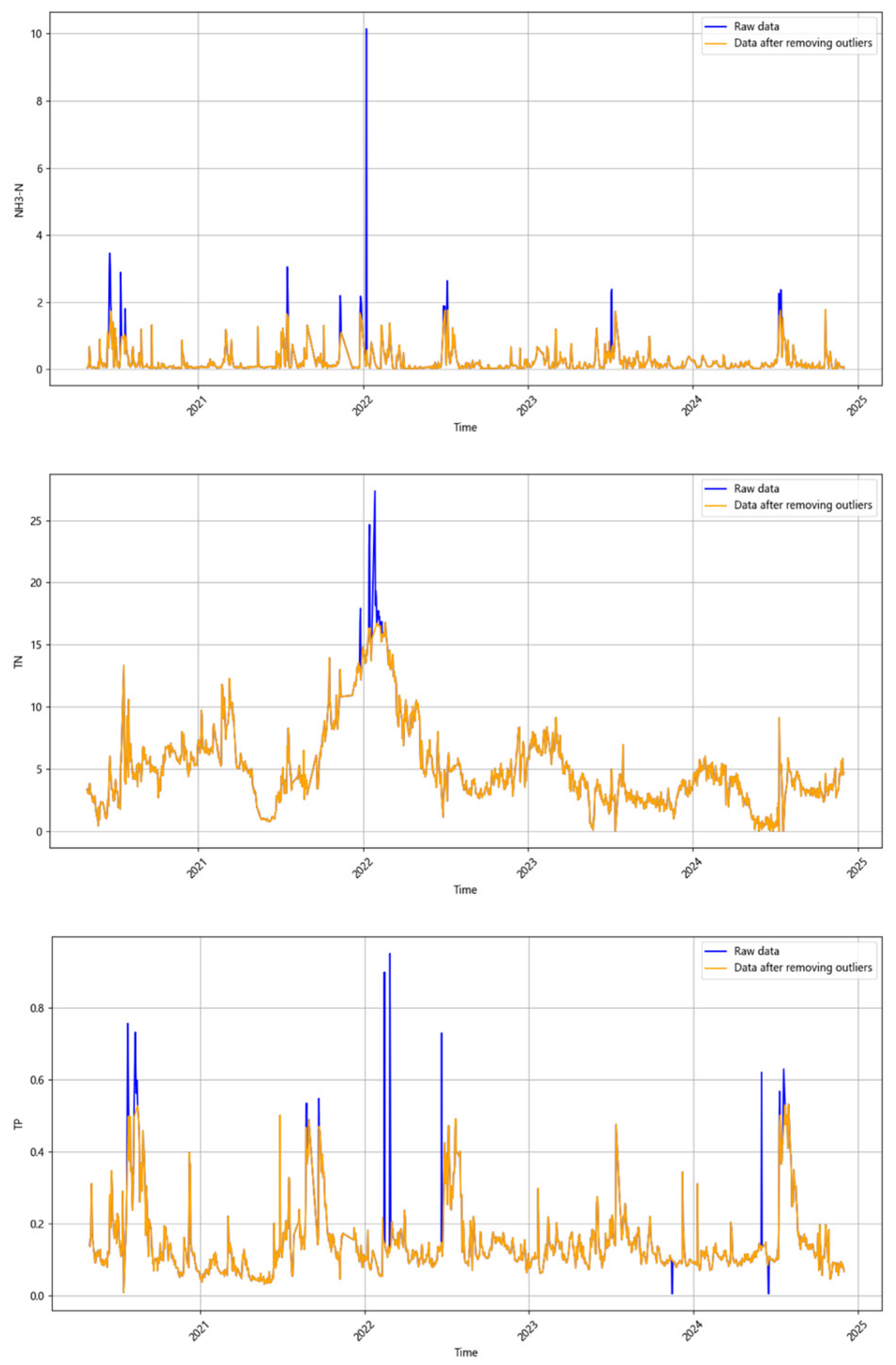
2.3. Outlier Handling

In the process of data collection, water quality time series data may contain outliers, defined as data points that deviate significantly from the majority of observations and are likely caused by non-representative events or errors. In this study, outliers are characterized by anomalous values (extremely high or low) that do not reflect the typical dynamics of water quality parameters (NH₃-N, TN, TP). These deviations are primarily attributed to factors such as extreme weather events (e.g., intense rainfall causing unusual dilution or pollutant runoff spikes), instrument malfunctions, or data transmission errors. Such outliers can introduce substantial noise, disrupt the continuity of the dataset, and negatively impact the stability of model training and the accuracy of predictions.

This study employs the Isolation Forest algorithm to detect outliers [34].The isolated forest algorithm is an unsupervised machine learning technique that isolates anomalies by randomly selecting features and then randomly selecting the split between the maximum and minimum values of the selected features. These splits produce smaller subsets until each point is isolated in a separate partition. Because outliers are located in sparse areas of the data set, they are easier to isolate. The anomaly score is calculated using the number of partitions required to isolate a point.

The number of trees is set to 100, and the contamination ratio is set to 0.015. The detected outliers were removed, and linear interpolation was applied, with Figure 2 presenting the comparison of the three water quality indicators before and after processing. The raw time series data is plotted as a blue solid line, the data after removing the outliers is plotted as an orange solid line, and the comparison of the two clearly shows the outliers.

2.4. Data Normalization

To mitigate the influence of varying scales among water quality parameters, min-max normalization was applied to transform all features into a uniform range of [0, 1] [35]. This method preserves the relative relationships between data points while accelerating model convergence. The normalization formula is expressed as:

$$x_{\mathrm{norm}}={\displaystyle \frac{x-x_{\min }}{x_{\max }-x_{\min }}}$$

(2)

where $x_{norm}$ denotes the normalized data, and $x_{\min }$ and $x_{\max }$ denote the minimum and maximum values of each parameter in the training dataset, respectively. This step reduces computational complexity during training and enhances the stability of gradient updates, which is critical for handling the nonlinear dynamics in agricultural pollution time series.

3. Methods

3.1. Variational Mode Decomposition

Variational mode decomposition (VMD) is an adaptive signal decomposition method designed to decompose a complex signal $f\left(t\right)$ into a set of quasi-orthogonal intrinsic mode functions (IMFs) with sparse spectral representations [36]. The core idea of VMD is to formulate a constrained variational optimization problem, where each IMF $u_k\left(t\right)$ is compact around a central frequency $w_k$, and the sum of all IMFs reconstructs the original signal. The VMD algorithm seeks to minimize the total bandwidth of all IMFs while ensuring their summation equals the original signal. The optimization problem is defined as:

$$\left\{\begin{array}{c}{\min }_{\left\{u_k\right\},\left\{{\omega }_k\right\}}{\displaystyle \sum _{k=1}^K{‖{\partial }_t\left[\left(\delta (t)+\frac{j}{\pi t}\right)⁎u_k(t)\right]e^{-j{\omega }_{k}t}‖}_2^2}\\ \mathrm{s}.\mathrm{t}.{\displaystyle \sum _{k=1}^K{u}_k(t)}=f(t)\end{array}\right.$$

(3)

where $K$ is the predefined number of IMFs, ${\partial }_t$ denotes the time derivative, $\delta \left(t\right)$ is the Dirac delta function, ⁎ represents convolution, and j is the imaginary unit. The analytic signal of $u_k\left(t\right)$, generated by the Hilbert transform $\left(\delta \left(t\right)+{\displaystyle \frac{j}{\pi t}}\right)⁎u_k\left(t\right)$, is shifted to the baseband via $e^{-j{w}_{k}t}$ [37]. The $L^2$- norm of its gradient quantifies the compactness of the IMF around $w_k$.

To solve the constrained problem, an augmented Lagrangian function $\mathcal{L}$ is introduced with a quadratic penalty term $\alpha$ and a Lagrangian multiplier $\lambda \left(t\right)$:

$$\mathcal{L}=\alpha {\displaystyle \sum _{k=1}^K{‖{\partial }_t\left[\left(\delta (t)+\frac{j}{\pi t}\right)⁎u_k(t)\right]e^{-j{\omega }_{k}t}‖}_2^2}+{‖f(t)-{\displaystyle \sum _{k=1}^K{u}_k(t)}‖}_2^2+\langle \lambda (t),f(t)-{\displaystyle \sum _{k=1}^K{u}_k(t)}\rangle$$

(4)

where $\alpha$ controls the bandwidth of IMFs (higher $\alpha$ enforces tighter frequency localization), and $〈 , 〉$ denotes the inner product.

The problem is efficiently solved in the frequency domain using the Alternating Direction Method of Multipliers (ADMM) [38]. The steps are:

1.

Each IMF $u_k\left(w\right)$ in the frequency domain is updated as:

$$u_k^{n+1}\left(\omega \right)={\displaystyle \frac{f\left(\omega \right)-{\displaystyle \sum _{i¡\ne k}{u}_i\left(w\right)}+\frac{\lambda \left(\omega \right)}{2}}{1+2\alpha {\left(\omega -{\omega }_k^n\right)}^2}}$$

(5)

where $f\left(w\right)$ is the Fourier transform of $f\left(t\right)$, and the denominator enforces spectral sparsity around $w_k$.

2.

The central frequency $w_k$ is updated as the centroid of the corresponding IMF power spectrum:

$${\omega }_k^{n+1}={\displaystyle \frac{{\displaystyle {\int }_0^{\infty }\omega }|u_k^{n+1}\left(\omega \right){|}^{2}d\omega }{{\displaystyle {\int }_0^{\infty }|}{u}_k^{n+1}\left(\omega \right){|}^{2}d\omega }}$$

(6)

3.

The Lagrangian multiplier $\lambda \left(w\right)$ is updated to penalize reconstruction errors:

$${\lambda }^{n+1}\left(\omega \right)={\lambda }^n\left(\omega \right)+\tau \left(f\left(\omega \right)-{\displaystyle \sum _{k=1}^K{u}_k^{n+1}}\left(\omega \right)\right)$$

(7)

where $\tau$ is the step size.

4.

The iteration stops when the relative change in IMFs falls below a tolerance ϵ:

$${\displaystyle \sum _{k=1}^K\frac{\Vert u_k^{n+1}-u_k^n{\Vert }_2^2}{\Vert u_k^n{\Vert }_2^2}<ϵ}$$

(8)

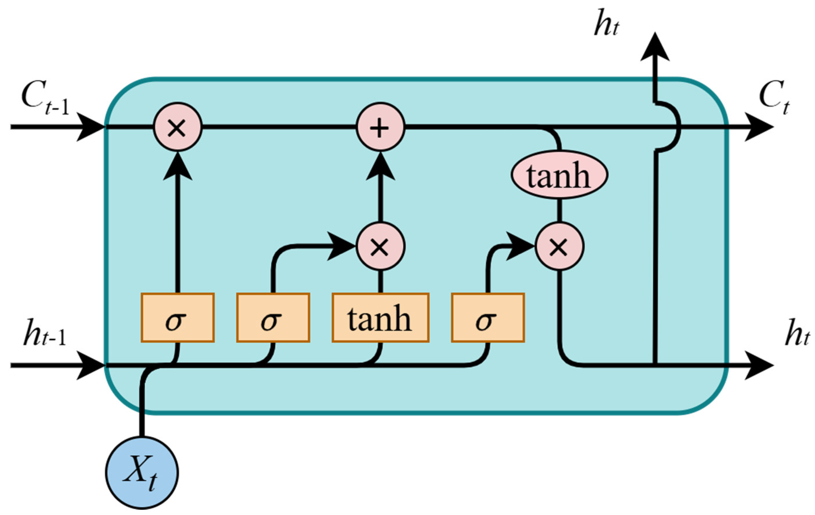
3.2. Long Short-Term Memory Networks

Long short-term memory (LSTM) networks are a type of recurrent neural network (RNN) designed to address the issues of vanishing and exploding gradients that are common in traditional RNNs [39]. An LSTM unit comprises three gates—forget gate, input gate, and output gate—that regulate information flow within the cell, and the structure is shown in Figure 3.

The forget gate determines which information to discard from the cell state $C_{t-1}$. It uses a sigmoid activation function to generate a value between 0 and 1, where 0 means “completely forget” and 1 means “completely retain”.

$$\sigma \left(x\right)={\displaystyle \frac{1}{1+e^{-x}}}$$

(9)

$$f_t=\sigma \left(W_f\cdot \left[h_{t-1},x_t\right]+b_f\right)$$

(10)

The input gate updates the cell state by filtering new information:

$$i_t=\sigma \left(W_i\cdot \left[h_{t-1},x_t\right]+b_i\right)$$

(11)

$$\tan \mathrm{h}\left(x\right)={\displaystyle \frac{1-e^{-2x}}{1+e^{-x}}}$$

(12)

$${\tilde{C}}_t=\tan \mathrm{h}\left(W_C\cdot \left[h_{t-1},x_t\right]+b_C\right)$$

(13)

The cell state update mechanism combines the previous state $C_{t-1}$ with the new candidate values ${\tilde{C}}_t$:

$$C_t=f_t\odot C_{t-1}+i_t\odot {\tilde{C}}_t$$

(14)

The output gate controls the output $h_t$ based on the updated cell state:

$$o_t=\sigma \left(W_o\cdot \left[h_{t-1},x_t\right]+b_o\right)$$

(15)

$$h_t=o_t\odot \tan \mathrm{h}\left(C_t\right)$$

(16)

where ⊙ represents element-wise multiplication, $W$ and $b$ are learnable weights and biases, $x_t$ is the input at time $t$, and $h_t$ is the hidden state.

3.3. Genetic Algorithm

To enhance the predictive performance of the LSTM network, a genetic algorithm (GA) was employed to optimize its hyperparameters. GA is a metaheuristic inspired by natural selection processes, characterized by its global search capability and robustness in navigating complex, nonlinear optimization landscapes [40].

The genetic algorithm followed an iterative “initialization-evaluation-evolution” cycle to optimize LSTM hyperparameters. During initialization, a population of 50 candidate solutions was generated, with each individual encoding hyperparameters including learning rate, number of hidden layers, units per layer, activation functions, batch size, and training epochs. In the evaluation phase, each candidate configuration underwent full LSTM training, with the mean absolute error (MAE) on a validation set serving as the fitness metric. Lower MAE values indicated higher fitness.

The evolutionary phase employed a hybrid strategy:

• Tournament selection: Groups of several individuals were randomly selected, retaining only the one with the best fitness to populate the mating pool. This approach effectively maintains population diversity while ensuring selection pressure, reducing premature convergence risks compared to roulette wheel selection [41].
• Arithmetic crossover: Parent hyperparameters were blended using domain-specific rules. Learning rates were averaged in logarithmic space, training epochs were integer-averaged, and activation functions were randomly inherited from either parent.
• Gaussian mutation: The learning rate was randomly adjusted according to a log-normal distribution, while the activation function and the number of training epochs were randomly replaced based on probability. This ensures the local search capability while maintaining the possibility of exploring new solution spaces [42].

The entire evolutionary process continuously optimizes the population quality through multiple generations of iterations and eventually converges to the parameter combination with the highest fitness.

3.4. VMD-GA-LSTM Model

The VMD-GA-LSTM model used in this study integrates variational mode decomposition (VMD) and genetic algorithm (GA)-optimized long short-term memory (LSTM) networks for predicting water quality parameters (ammonia, total phosphorus, and total nitrogen) in an agricultural watershed. This approach effectively combines the strengths of both decomposition techniques and deep learning models to enhance prediction accuracy and capture the intricate temporal dynamics associated with agricultural pollution in water bodies. The model framework is shown in Figure 4.

The proposed VMD-GA-LSTM framework for predicting water quality parameters can be formally expressed as follows:

$$IM{F}_k=VM{D}_k(X;K,\alpha )\hspace{1em}\forall k\in \{1,2,\dots ,K\}$$

(17)

where $X=[x_1,x_2,\dots ,x_T]$ is the input water quality time series, $K$ is the number of intrinsic mode functions (IMFs), and $\alpha$ is the bandwidth control parameter.

$${\widehat{IMF}}_k={\mathrm{LSTM}}_{{\theta }_k}({\mathrm{IMF}}_k)\hspace{1em}\forall k\in \{1,2,\dots ,K\}$$

(18)

where ${\mathrm{LSTM}}_{{\theta }_k}$ denotes the LSTM model predicting the k-th IMF component.

$$\widehat{Y}={\displaystyle \sum _{k=1}^K{\widehat{IMF}}_k}$$

(19)

where $\widehat{Y}=[{\widehat{y}}_{T+1},{\widehat{y}}_{T+2},\dots ,{\widehat{y}}_{T+H}]$ is the final predicted water quality series for $H$ future time steps.

The optimal hyperparameters ${\phi }^{⁎}$ for the ensemble of LSTM models are determined by the genetic algorithm to minimize the prediction error on a validation set:

$${\phi }^{⁎}=\arg {\min }_{\phi }\mathcal{L}(Y_{\mathrm{val}},{\widehat{Y}}_{\mathrm{val}}(\phi ))$$

(20)

where $\phi$ represents the hyperparameter configuration space (e.g., learning rate, number of layers, units per layer, batch size, epochs), $Y_{\mathrm{val}}$ is the ground truth in the validation set, ${\widehat{Y}}_{\mathrm{val}}(\phi )$ is the prediction using hyperparameter set $\phi$, and $\mathcal{L}$ is the loss function.

Thus, the final prediction model utilizes the optimal hyperparameters ${\phi }^{⁎}$ to configure the LSTM predictors:

$$\widehat{Y}={\displaystyle \sum _{k=1}^K{\mathrm{LSTM}}_{{\theta }_k}}({\phi }^{⁎})({\mathrm{VMD}}_k(X;K,\alpha ))$$

(21)

The key steps of the framework are as follows:

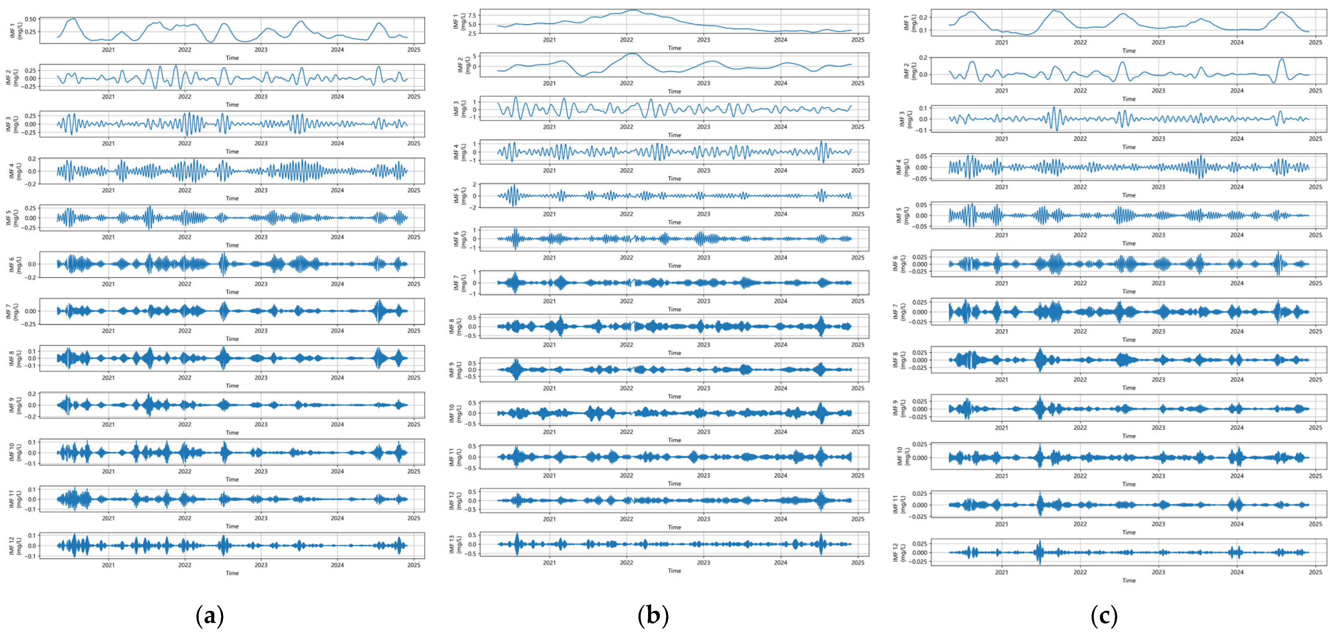
• The preprocessed water quality time series data is first decomposed using variational mode decomposition (VMD), splitting it into multiple intrinsic mode functions (IMFs). Each IMF represents a specific frequency component of the water quality parameters. This decomposition helps isolate different frequency characteristics in the data.
• After decomposition, each IMF is individually processed using long short-term memory (LSTM) networks. These LSTMs are trained separately for each IMF to capture short-term and long-term temporal dependencies. The LSTM model is optimized to minimize the prediction error, providing a forecast for each IMF.
• The convergence of each IMF-LSTM pair is achieved through iterative optimization. During training, the LSTM parameters (weights and biases) are adjusted to minimize the prediction error for each IMF, ensuring the model has captured the temporal dynamics. The convergence occurs when the error stabilizes to a minimum value, indicating effective model performance.
• A genetic algorithm (GA) is employed to optimize the hyperparameters of the LSTM networks for each IMF. The GA searches for the best set of parameters (e.g., learning rate, number of layers, batch size) by evaluating the LSTM performance through a fitness function.
• After each IMF is processed by its corresponding LSTM, the final water quality prediction is obtained by linearly summing the individual predictions of all IMFs. This summation combines the information from all frequency components, providing a comprehensive prediction of water quality parameters (NH₃-N, TP, TN).

3.5. Evaluation Indicators

To comprehensively assess the predictive performance of the VMD-LSTM model for NH₃-N, TN, and TP, three widely adopted evaluation metrics were employed: Root Mean Squared Error (RMSE), mean absolute error (MAE), and the Coefficient of Determination (R²). RMSE measures the average deviation between predicted values and observed values. It is particularly sensitive to outliers, and the smaller the value, the more accurate the prediction result. MAE provides the size of the mean absolute error, and again, the smaller it is, the more accurate it is. R² represents the degree of fit; the closer to 1 the better. These indicators quantify prediction accuracy, error magnitude, and model explanatory power, respectively, and are defined as follows:

$$\mathrm{RMSE}=\sqrt{{\displaystyle \frac{1}{n}}{\displaystyle \sum _{i=1}^n{\left(y_i-{\widehat{y}}_i\right)}^2}}$$

(22)

$$\mathrm{MAE}={\displaystyle \frac{1}{n}}{\displaystyle \sum _{i=1}^n}|y_i-{\widehat{y}}_i|$$

(23)

$$R^2=1-{\displaystyle \frac{{\displaystyle \sum _{i=1}^n{\left(y_i-{\widehat{y}}_i\right)}^2}}{{\displaystyle \sum _{i=1}^n{\left(y_i-\overline{y}\right)}^2}}}$$

(24)

where $n$ is the number of samples, $y_i$ is the measured value, ${\widehat{y}}_i$ is the predicted value, and $\overline{y}$ is the average value of the measured data.

3.6. Experimental Environment

The experimental setup utilized a Xiaomi laptop (manufactured by Xiaomi Inc., Beijing, China) equipped with a 12th Gen Intel Core i7-12650H CPU and an NVIDIA GeForce RTX 2050 GPU to accelerate deep learning computations. The software environment was configured on a Windows 11 64-bit operating system, with TensorFlow 2.12.0 as the core deep learning framework, leveraging CUDA 11.8 and cuDNN 8.6.0 libraries for GPU-accelerated training.

4. Results and Discussion

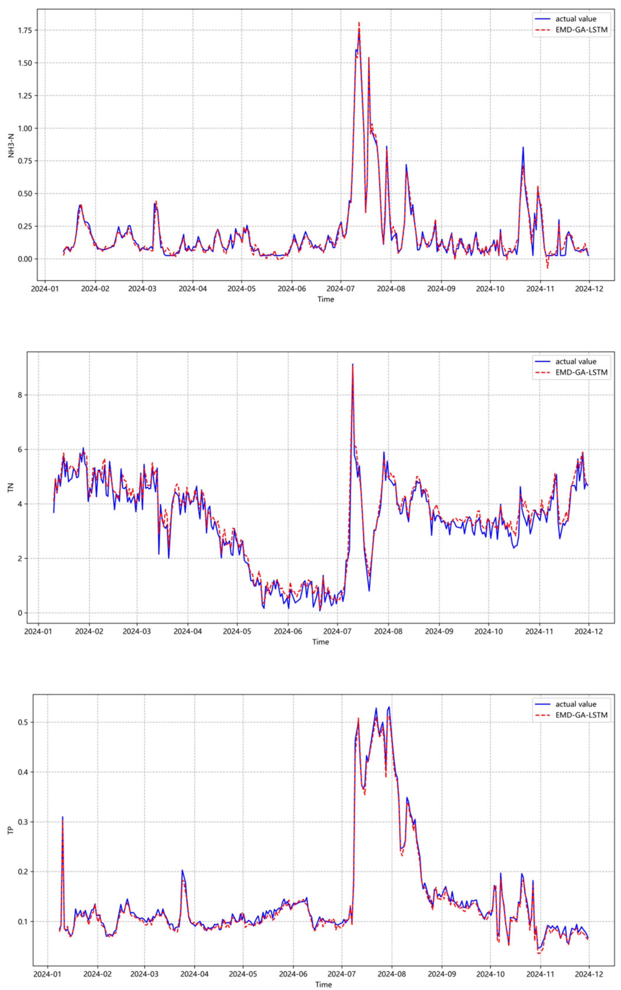
4.1. Empirical Analysis of EMD-GA-LSTM Model

After data preprocessing, the VMD method was used to decompose the time series data of ammonia nitrogen (NH₃-N), total nitrogen (TN), and total phosphorus (TP) water quality. The performance of VMD critically depends on two key parameters: the number of modes K and the bandwidth penalty factor α. Improper selection of K may lead to under-decomposition (insufficient separation of signal components) or over-decomposition (redundant modes containing noise), while an inappropriate α can result in either excessive mode overlap in the frequency domain or loss of signal details [43]. In this study, the optimal parameters for NH₃-N were determined by the iterative trial-and-error method combined with quantitative assessment to be K = 12 and α = 2000, for TN to be K = 13 and α = 2000, and for TP to be K = 12 and α = 2000.

The decomposition process produces multiple intrinsic mode functions (IMFs), where IMF1 represents the lowest-frequency component, and higher-indexed IMFs progressively capture higher-frequency oscillations. The lowest frequency IMF reflects long-term trends and provides valuable information for understanding the general direction of water quality change. The decomposition results are shown in Figure 5.

The VMD decomposition of the TN time series shows an increase in the low-frequency component (i.e., IMF1) between 2020 and early 2022, followed by a clear decrease in the following years. The early uptick may be related to heightened agricultural activity during the COVID-19 pandemic. The epidemic led to a decline in agricultural total factor productivity, and the main way to make up for the loss of total factor productivity was to increase advanced input factors such as fertilizers and machinery [44]. More nitrogen fertilizer naturally led to an increase in TN. The decline after 2022 may reflect the effect of strengthened policies. China has strengthened the control of agricultural non-point source pollution in the 14th Five-Year Plan (2021–2025), especially the control of pollution from fertilizers, livestock, and poultry breeding. In addition, the “Implementation Plan for Agricultural Non-point Source Pollution Control and Supervision Guidance” released in 2021 pointed out that it would focus on supporting the reduction and efficiency increase of fertilizers and pesticides and require the reduction of nitrogen and phosphorus loss loads.

Unlike the low-frequency component of TN, which significantly increased and then decreased, the IMF1 components of NH₃-N and TP did not show an intuitive trend. However, quantitative analysis based on linear regression showed a statistically significant negative trend in both IMF1 components. This downward trend suggests that stricter nitrogen and phosphorus emissions regulations and better agricultural management practices aimed at reducing nutrient loads have had a positive impact. Since China implemented the Water Pollution Prevention and Control Action Plan in 2015, it has included total phosphorus in key control indicators and strengthened restrictions on phosphate fertilizers and supervision of pollution discharge.

The dataset spanning from May 2020 to November 2024 was partitioned into training (80%) and testing (20%) sets, maintaining temporal continuity to avoid data leakage. To assess model robustness and hyperparameter stability, we implemented a 5-fold cross-validation within the training set. Prior to forecasting, the structure and parameters of the VMD-GA-LSTM prediction model were optimally estimated by a genetic algorithm. After empirical testing of window sizes (8, 10, 12, 14), a time window of 10 historical steps was selected as optimal for capturing short-term temporal dependencies in water quality dynamics. The Adam optimizer was uniformly adopted for all models due to its adaptive learning rate capabilities and computational efficiency [45]. For each prediction target, independent hyperparameter optimization was conducted to account for the distinct temporal dynamics and nonlinear relationships inherent in each indicator. The hyperparameter search space for genetic algorithm optimization is defined as follows: (i) learning rate: {0.1, 0.01, 0.001, 0.0001}; (ii) hidden layers: {1, 2, 3, 4}; (iii) units per layer: {50, 100, 200,300}; (iv) activation functions: ReLU and Tanh; (v) batch size: {16, 32, 48, 64}; and (vi) training epochs: {10, 20… 80}.

Table 1. Five-fold cross-validation results (mean ± std) on training set.

Water Quality Indicators	RMSE	MAE	R2
NH3-N	0.019 ± 0.002	0.014 ± 0.001	0.994 ± 0.003
TN	0.136 ± 0.008	0.104 ± 0.006	0.993 ± 0.002
TP	0.004 ± 0.000	0.003 ± 0.000	0.995 ± 0.001

reports the mean ± standard deviation of RMSE, MAE, and R² across all folds, demonstrating consistent performance. The optimal hyperparameter configuration of the predictive model explored is shown in

Table 2. Optimal hyperparameter configurations for NH₃-N, TN, and TP prediction models.

Parameter	Meaning	NH3-N	TN	TP
Learning rate	Controls the step size for updating model weights	0.001	0.001	0.001
Hidden layer	The number of intermediate layers in the neural network	1	1	1
Units	The number of neurons in each hidden layer	300	200	100
Activation	The activation function	Tanh	Tanh	Tanh
Batch size	The number of samples used in each training iteration	16	32	16
Epochs	The number of dataset iterations during training	50	60	60

.

Cross-validation demonstrated robust performance across folds, and final test results aligned closely with cross-validation metrics. The VMD-GA-LSTM model achieved an RMSE of 0.019, an MAE of 0.014, and an R² of 0.994 for NH₃-N on the test set. Similarly, TN predictions showed strong generalizability, attaining a testing RMSE of 0.152 (MAE: 0.115, R²: 0.990). TP predictions exhibited the highest precision, with a testing RMSE at 0.007 (MAE: 0.005, R²: 0.993). Figure 6 illustrates the prediction results of each prediction model for each of the three water quality indicators.

4.2. Model Comparison

In order to fully verify the superiority of the VMD-GA-LSTM model in the prediction of water quality pollution from agricultural non-point sources, the LSTM model, back propagation neural network (BPNN) model, support vector regression (SVR) model, and EMD-LSTM model were selected for experimental comparison. RMSE, MAE, and R2 were used as evaluation indexes, and the prediction results of each model are shown in

Table 3. Model evaluation results.

Water Quality Indicators	Model	RMSE	MAE	R2
NH3-N	SVR	0.129	0.069	0.697
	BP	0.127	0.073	0.712
	LSTM	0.120	0.067	0.741
	EMD-LSTM	0.041	0.029	0.975
	VMD-GA-LSTM	0.024	0.017	0.991
TN	SVR	0.758	0.435	0.763
	BP	0.840	0.551	0.712
	LSTM	0.737	0.434	0.778
	EMD-LSTM	0.332	0.251	0.955
	VMD-GA-LSTM	0.152	0.115	0.990
TP	SVR	0.034	0.020	0.877
	BP	0.037	0.024	0.853
	LSTM	0.033	0.015	0.886
	EMD-LSTM	0.011	0.008	0.988
	VMD-GA-LSTM	0.007	0.005	0.993

.

SVR and BPNN exhibited the highest errors, particularly for TN and NH₃-N, due to their inability to resolve the multi-scale temporal dependencies inherent in agricultural runoff. While standalone LSTM reduced TN RMSE by 12.9% compared to SVR, its R² remained ≤0.886, highlighting spectral insensitivity to high-frequency noise and low-frequency trends. EMD-LSTM showed significant improvement, with much better prediction accuracy for all three water quality metrics compared to LSTM, verifying the necessity of signal decomposition for noise separation. However, the mixing of residual modes in EMD also leaves the method with room for improvement.

The proposed VMD-GA-LSTM model showed higher prediction accuracy for all three water quality indicators (NH₃-N, TN, and TP) compared with the other selected models. Compared to second-best model (EMD-LSTM), VMD-GA-LSTM reduced the average RMSE by 41.5% (NH₃-N), 54.2% (TN), and 36.4% (TP) and the MAE by 41.4% (NH₃-N), 54.2% (TN), and 37.5% (TP). R² enhancement was 0.016 (NH₃-N), 0.035 (TN), 0.005 (TP). These results highlight that combining variational mode decomposition with LSTM can effectively address the non-stationarity and nonlinearity issues in agricultural non-point source water quality data.

4.3. Sensitivity Analysis on Data Noise Robustness

To evaluate the robustness of the VMD-GA-LSTM model against data perturbations, Gaussian noise with varying intensities was introduced to the original water quality time series. The noise was generated with a mean of zero and standard deviations equivalent to 5% and 10% of the original data’s standard deviation. The performance metrics (RMSE, MAE, and R²) were recalculated and compared against the baseline (noise-free testing data).

Table 4. Sensitivity of prediction errors to data noise.

Water Quality Indicators	Noise Level	RMSE	MAE	R2
NH3-N	0% (Baseline)	0.024	0.017	0.991
	5%	0.025	0.019	0.990
	10%	0.025	0.022	0.987
TN	0% (Baseline)	0.152	0.115	0.990
	5%	0.154	0.120	0.988
	10%	0.159	0.122	0.985
TP	0% (Baseline)	0.007	0.005	0.993
	5%	0.007	0.005	0.991
	10%	0.009	0.007	0.989

summarizes the prediction errors under different noise levels. For NH₃-N, RMSE remained stable (≤4.2% increase) under noise, indicating strong noise resilience. TN exhibited gradual error increments (≤4.6%), reflecting its capacity to absorb perturbations in complex temporal dynamics. The sensitivity of TP was slightly higher compared to NH₃-N and TN, which may be due to the fact that the value of baseline was too low to amplify the effect of noise. Despite this, all R² values exceeded 0.985, confirming robust predictive performance. The VMD-GA-LSTM framework exhibited sufficient robustness to handle realistic data imperfections, reinforcing its applicability in practical agricultural water quality management scenarios.

4.4. Policy Recommendations for Sustainable Agricultural Management

Based on the VMD-GA-LSTM predictions and observed trends in NH₃-N, TN, and TP concentrations, the following policy recommendations are proposed to mitigate agricultural non-point source pollution and promote sustainable watershed management:

4.4.1. Precision Agriculture Practices

The temporal patterns of NH₃-N and TP low-frequency components highlight the critical influence of fertilizer application timing and intensity on water quality. Implementing precision agriculture techniques can optimize fertilizer use efficiency and reduce water pollution. Predictive models like VMD-GA-LSTM can be integrated into decision-support systems to forecast seasonal nutrient demands, enabling farmers to dynamically adjust fertilizer application rates. More reasonable fertilization technology can effectively reduce pollution and achieve sustainable agricultural development [46].

4.4.2. Policy Incentives for Circular Agricultural Systems

Circular agriculture focuses on producing agricultural products using minimal external inputs, closing the nutrient cycle, and reducing negative emissions to the environment [47].The continued decline in the low-frequency components of TN after 2022 reflects the effectiveness of China’s circular agriculture system. Subsidies for slow-release fertilizers, biochar-enhanced compost [48], and livestock manure recycling systems could then be expanded to incentivize circular agriculture and reduce pollution. The VMD-GA-LSTM model could be integrated into a regional decision support system, which would simulate the impact of different policy incentives, such as subsidies or regulations on fertilizer use, on water quality at both farm and regional levels. The system could help policymakers assess the effectiveness of various interventions in improving water quality and reducing agricultural non-point source pollution.

4.4.3. Farmer Education and Cross-Sectoral Collaboration

Limited technical knowledge and economic barriers hinder adoption of sustainable practices. Multidisciplinary extension programs should train farmers in climate-smart practices, such as training them to interpret pollution alerts via mobile platforms so they can proactively adjust irrigation and fertilization schedules. Additionally, fostering collaboration between agricultural cooperatives, environmental agencies, and AI developers can accelerate the co-design of context-specific pollution mitigation strategies. By integrating VMD-GA-LSTM model predictions into educational platforms, farmers can receive real-time feedback on water quality, empowering them to make data-driven decisions. The dashboard could include features such as forecasting pollution levels and providing recommendations on when to adjust fertilizer application based on model predictions.

5. Conclusions

This study constructed an agricultural non-point source water quality prediction model based on VMD-GA-LSTM to address the challenges brought by the nonlinearity and non-stationarity of water quality time series. By combining variational mode decomposition with deep learning, the model effectively captured both short-term fluctuations and long-term trends in water quality dynamics. A genetic algorithm was introduced to adaptively optimize the hyperparameter combinations of LSTM models, which significantly improved the prediction accuracy and robustness. The decomposition of TN time series revealed an initial increase in the low-frequency component during the COVID-19 pandemic, likely linked to intensified fertilizer use, followed by a post-2022 decline attributable to China’s strengthened agricultural pollution control policies. In contrast, the low-frequency components of NH₃-N and TP exhibited a consistent downward trajectory, reflecting the long-term success of related pollution prevention and control actions.

By comparing the RMSE, MAE, and R² of various models, the results show that the VMD-GA-LSTM model has the lowest error and extremely high accuracy, indicating that using VMD to decompose the sequence into different components can significantly improve the accuracy. From a policy perspective, the predictive capabilities of the VMD-GA-LSTM model provide actionable insights for sustainable agricultural practices. Precision agriculture, optimized fertilizer scheduling, and circular farming systems—supported by real-time monitoring and predictive analytics—are critical to mitigating non-point source pollution. Additionally, farmer education and cross-sector collaboration are essential to scale adoption of eco-friendly practices, ensuring alignment with national pollution control targets.

In future studies, we will explore and implement more systematic or automated methods for determining optimal VMD parameters. This will address the current reliance on empirical trial-and-error and significantly improve the reproducibility, robustness, and ease of application of the model. We will also undertake a dedicated effort to benchmark it against a broader range of state-of-the-art (SOTA) models. This includes more recent deep learning architectures and sophisticated hybrid models reported in the recent literature. This comparative analysis will offer deeper insights into the specific strengths and potential limitations of our approach under varying data conditions. The development and implementation of these enhancements will leverage algorithmic optimizations and evolving hardware capabilities to improve computational efficiency and runtime performance.

References

1. Zahoor, I.; Mushtaq, A. Water pollution from agricultural activities: A critical global review. Int. J. Chem. Biochem. Sci. 2023, 23, 164–176. [Google Scholar]
2. Cooper, C. Biological effects of agriculturally derived surface water pollutants on aquatic systems—A review. J. Environ. Qual. 1993, 22, 402–408. [Google Scholar] [CrossRef]
3. Hussain, F.; Ahmed, S.; Muhammad Zaigham Abbas Naqvi, S.; Awais, M.; Zhang, Y.; Zhang, H.; Raghavan, V.; Zang, Y.; Zhao, G.; Hu, J. Agricultural Non-Point Source Pollution: Comprehensive Analysis of Sources and Assessment Methods. Agriculture 2025, 15, 531. [Google Scholar] [CrossRef]
4. Juncal, M.J.L.; Masino, P.; Bertone, E.; Stewart, R.A. Towards nutrient neutrality: A review of agricultural runoff mitigation strategies and the development of a decision-making framework. Sci. Total Environ. 2023, 874, 162408. [Google Scholar] [CrossRef] [PubMed]
5. Zhang, J.; Xiao, H.; Fang, H. Component-based reconstruction prediction of runoff at multi-time scales in the source area of the Yellow River based on the ARMA model. Water Resour. Manag. 2022, 36, 433–448. [Google Scholar] [CrossRef]
6. Montanari, A.; Rosso, R.; Taqqu, M.S. Fractionally differenced ARIMA models applied to hydrologic time series: Identification, estimation, and simulation. Water Resour. Res. 1997, 33, 1035–1044. [Google Scholar] [CrossRef]
7. Thoe, W.; Lee, J.H. Daily forecasting of Hong Kong beach water quality by multiple linear regression models. J. Environ. Eng. 2014, 140, 04013007. [Google Scholar] [CrossRef]
8. Faruk, D.Ö. A hybrid neural network and ARIMA model for water quality time series prediction. Eng. Appl. Artif. Intell. 2010, 23, 586–594. [Google Scholar] [CrossRef]
9. Chen, Y.; Song, L.; Liu, Y.; Yang, L.; Li, D. A review of the artificial neural network models for water quality prediction. Appl. Sci. 2020, 10, 5776. [Google Scholar] [CrossRef]
10. Karthikeyan, L.; Kumar, D.N. Predictability of nonstationary time series using wavelet and EMD based ARMA models. J. Hydrol. 2013, 502, 103–119. [Google Scholar] [CrossRef]
11. Zhang, F.; O’Donnell, L.J. Support vector regression. In Machine Learning; Elsevier: Amsterdam, The Netherlands, 2020; pp. 123–140. [Google Scholar] [CrossRef]
12. Pham, L.T.; Luo, L.; Finley, A.O. Evaluation of Random Forest for short-term daily streamflow forecast in rainfall and snowmelt driven watersheds. Hydrol. Earth Syst. Sci. Discuss. 2020, 25, 2997–3015. [Google Scholar] [CrossRef]
13. Neu, D.A.; Lahann, J.; Fettke, P. A systematic literature review on state-of-the-art deep learning methods for process prediction. Artif. Intell. Rev. 2022, 55, 801–827. [Google Scholar] [CrossRef]
14. Han, Z.; Zhao, J.; Leung, H.; Ma, K.F.; Wang, W. A review of deep learning models for time series prediction. IEEE Sens. J. 2019, 21, 7833–7848. [Google Scholar] [CrossRef]
15. Bi, J.; Lin, Y.; Dong, Q.; Yuan, H.; Zhou, M. Large-scale water quality prediction with integrated deep neural network. Inf. Sci. 2021, 571, 191–205. [Google Scholar] [CrossRef]
16. Mengdi, Z.; Qing, X.; Zhenhong, L.; Chunyan, M.; Pin, G. Prediction of water quality time series based on the dynamic sliding window BP neural network model. J. Environ. Eng. Technol. 2022, 12, 809–815. [Google Scholar] [CrossRef]
17. Li, L.; Jiang, P.; Xu, H.; Lin, G.; Guo, D.; Wu, H. Water quality prediction based on recurrent neural network and improved evidence theory: A case study of Qiantang River, China. Environ. Sci. Pollut. Res. 2019, 26, 19879–19896. [Google Scholar] [CrossRef]
18. Noh, S.-H. Analysis of gradient vanishing of RNNs and performance comparison. Information 2021, 12, 442. [Google Scholar] [CrossRef]
19. Landi, F.; Baraldi, L.; Cornia, M.; Cucchiara, R. Working memory connections for LSTM. Neural Netw. 2021, 144, 334–341. [Google Scholar] [CrossRef]
20. Li, Q.; Yang, Y.; Yang, L.; Wang, Y. Comparative analysis of water quality prediction performance based on LSTM in the Haihe River Basin, China. Environ. Sci. Pollut. Res. 2023, 30, 7498–7509. [Google Scholar] [CrossRef]
21. Farhi, N.; Kohen, E.; Mamane, H.; Shavitt, Y. Prediction of wastewater treatment quality using LSTM neural network. Environ. Technol. Innov. 2021, 23, 101632. [Google Scholar] [CrossRef]
22. Gao, Z.; Chen, J.; Wang, G.; Ren, S.; Fang, L.; Yinglan, A.; Wang, Q. A novel multivariate time series prediction of crucial water quality parameters with Long Short-Term Memory (LSTM) networks. J. Contam. Hydrol. 2023, 259, 104262. [Google Scholar] [CrossRef] [PubMed]
23. Doğan, E. Robust-LSTM: A novel approach to short-traffic flow prediction based on signal decomposition. Soft Comput. 2022, 26, 5227–5239. [Google Scholar] [CrossRef]
24. Xu, R.; Hu, S.; Wan, H.; Xie, Y.; Cai, Y.; Wen, J. A unified deep learning framework for water quality prediction based on time-frequency feature extraction and data feature enhancement. J. Environ. Manag. 2024, 351, 119894. [Google Scholar] [CrossRef] [PubMed]
25. Yang, M.; Tong, L.; Xia, A.; Fang, K. A multi-factor water quality prediction method based on wavelet transform and lstm. In Proceedings of the International Conference on Heterogeneous Networking for Quality, Reliability, Security and Robustness, Shenzhen, China, 8–9 October 2023; pp. 130–144. [Google Scholar] [CrossRef]
26. Junsheng, C.; Dejie, Y.; Yu, Y. Research on the intrinsic mode function (IMF) criterion in EMD method. Mech. Syst. Signal Process. 2006, 20, 817–824. [Google Scholar] [CrossRef]
27. Zhang, Y.; Li, C.; Jiang, Y.; Sun, L.; Zhao, R.; Yan, K.; Wang, W. Accurate prediction of water quality in urban drainage network with integrated EMD-LSTM model. J. Clean. Prod. 2022, 354, 131724. [Google Scholar] [CrossRef]
28. Dong, J.; Zhang, Y.; Hu, J. Short-term air quality prediction based on EMD-transformer-BiLSTM. Sci. Rep. 2024, 14, 20513. [Google Scholar] [CrossRef]
29. Yujun, Y.; Yimei, Y.; Wang, Z. Research on a hybrid prediction model for stock price based on long short-term memory and variational mode decomposition. Soft Comput. 2021, 25, 13513–13531. [Google Scholar] [CrossRef]
30. Ding, T.; Wu, D.a.; Shen, L.; Liu, Q.; Zhang, X.; Li, Y. Prediction of significant wave height using a VMD-LSTM-rolling model in the South Sea of China. Front. Mar. Sci. 2024, 11, 1382248. [Google Scholar] [CrossRef]
31. Wei, Y.; Qiao, X.; Zhang, Z.; Yang, Y.; Niu, H. Trade-off and driving mechanisms for farmland ecosystem services basedon climatic zones and agricultural regionalization. Trans. Chin. Soc. Agric. Eng. 2022, 38, 220–228. (In Chinese) [Google Scholar]
32. Dębska, K.; Rutkowska, B.; Szulc, W.; Gozdowski, D. Changes in selected water quality parameters in the Utrata River as a function of catchment area land use. Water 2021, 13, 2989. [Google Scholar] [CrossRef]
33. Gnauck, A. Interpolation and approximation of water quality time series and process identification. Anal. Bioanal. Chem. 2004, 380, 484–492. [Google Scholar] [CrossRef] [PubMed]
34. Liu, F.T.; Ting, K.M.; Zhou, Z.-H. Isolation-based anomaly detection. ACM Trans. Knowl. Discov. Data (TKDD) 2012, 6, 3. [Google Scholar] [CrossRef]
35. Ali, P.J.M.; Faraj, R.H.; Koya, E.; Ali, P.J.M.; Faraj, R.H. Data normalization and standardization: A technical report. Mach. Learn. Tech. Rep. 2014, 1, 1–6. [Google Scholar] [CrossRef]
36. Liu, Y.; Yang, G.; Li, M.; Yin, H. Variational mode decomposition denoising combined the detrended fluctuation analysis. Signal Process. 2016, 125, 349–364. [Google Scholar] [CrossRef]
37. Kurbatsky, V.G.; Sidorov, D.N.; Spiryaev, V.A.; Tomin, N.V. Forecasting nonstationary time series based on Hilbert-Huang transform and machine learning. Autom. Remote Control 2014, 75, 922–934. [Google Scholar] [CrossRef]
38. Boyd, S.; Parikh, N.; Chu, E.; Peleato, B.; Eckstein, J. Distributed optimization and statistical learning via the alternating direction method of multipliers. Found. Trends Mach. Learn. 2011, 3, 1–122. [Google Scholar] [CrossRef]
39. Sherstinsky, A. Fundamentals of recurrent neural network (RNN) and long short-term memory (LSTM) network. Phys. D Nonlinear Phenom. 2020, 404, 132306. [Google Scholar] [CrossRef]
40. Ding, S.; Su, C.; Yu, J. An optimizing BP neural network algorithm based on genetic algorithm. Artif. Intell. Rev. 2011, 36, 153–162. [Google Scholar] [CrossRef]
41. Shapiro, J. Genetic algorithms in machine learning. In Advanced Course on Artificial Intelligence; Springer: Cham, Switzerland, 1999; pp. 146–168. [Google Scholar] [CrossRef]
42. Saravanan, N.; Fogel, D.B.; Nelson, K.M. A comparison of methods for self-adaptation in evolutionary algorithms. BioSystems 1995, 36, 157–166. [Google Scholar] [CrossRef]
43. Zhang, X.; Miao, Q.; Zhang, H.; Wang, L. A parameter-adaptive VMD method based on grasshopper optimization algorithm to analyze vibration signals from rotating machinery. Mech. Syst. Signal Process. 2018, 108, 58–72. [Google Scholar] [CrossRef]
44. Zhang, S.; Wang, S.; Yuan, L.; Liu, X.; Gong, B. The impact of epidemics on agricultural production and forecast of COVID-19. China Agric. Econ. Rev. 2020, 12, 409–425. [Google Scholar] [CrossRef]
45. Kingma, D.P.; Ba, J. Adam: A method for stochastic optimization. arXiv 2014, arXiv:1412.6980. [Google Scholar] [CrossRef]
46. Xu, H.; Tan, X.; Liang, J.; Cui, Y.; Gao, Q. Impact of agricultural non-point source pollution on river water quality: Evidence from China. Front. Ecol. Evol. 2022, 10, 858822. [Google Scholar] [CrossRef]
47. Zadgaonkar, L.A.; Darwai, V.; Mandavgane, S.A. The circular agricultural system is more sustainable: Emergy analysis. Clean Technol. Environ. Policy 2022, 24, 1301–1315. [Google Scholar] [CrossRef]
48. Wang, C.; Luo, D.; Zhang, X.; Huang, R.; Cao, Y.; Liu, G.; Zhang, Y.; Wang, H. Biochar-based slow-release of fertilizers for sustainable agriculture: A mini review. Environ. Sci. Ecotechnol. 2022, 10, 100167. [Google Scholar] [CrossRef]
Figure 1. Study area.
Mathematics 13 01951 g001
Figure 2. Outlier handling results.
Mathematics 13 01951 g002
Figure 3. Structure of LSTM.
Mathematics 13 01951 g003
Figure 4. The framework of the VMD-GA-LSTM prediction model.
Mathematics 13 01951 g004
Figure 5. VMD decomposition results of the (a) NH3-N, (b) TN, and (c) TP time series.
Mathematics 13 01951 g005
Figure 6. VMD-GA-LSTM model prediction results.
Mathematics 13 01951 g006