The Well-Posedness and Ergodicity of a CIR Equation Driven by Pure Jump Noise

Abstract

The current paper is devoted to the dynamical property of the stochastic Cox–Ingersoll–Ross (CIR) model with pure jump noise, which is an extension of the CIR model. Firstly, we characterize the existence and 2-moment of the CIR process with a pure jump process. Consequently, we provide sufficient conditions for the compensated Poisson random measure under which the CIR process with a pure jump process is ergodic. Moreover, the stationary solution can be constructed from the invariant measure. Some numerical simulations are provided to visualize the theoretical results.

1. Introduction

Modeling the term structure of interest rates is a long-standing topic in financial economics. Many stochastic interest rate models have been proposed in the past decades to provide a realistic and tractable method of describing the term structure; some early contributions include Vasicek [1], Dothan [2], Cox et al. [3], and Hull-White [4]. If the interest rate is determined by only one stochastic differential equation, the model is referred to as a one-factor model. Cox et al. [3] assume that the evolution of the interest rate dynamics and the stochastic volatility is given by

$$\begin{array}{c}\hfill \mathrm{d}r\left(t\right)=k(\theta -r\left(t\right))\mathrm{d}t+ϵ\sqrt{r\left(t\right)}\mathrm{d}B\left(t\right),r\left(0\right)=r_0,\end{array}$$

(1)

where the constants $\theta ,k,ϵ$ characterize the long time mean, the volatility, and the speed of adjustment, respectively. In the classical case, $B\left(t\right)$ is assumed to be the standard Brownian motion. The stochastic differential equation (SDE) defined by (1) is said to be a CIR model. It is well known that the CIR model (1) is nonnegative and has some empirically relevant properties. In this model, when $k>0$, the interest rate $r\left(t\right)$ has a light-tailed stationary distribution; when $k<0$, the interest rate $r\left(t\right)$ does not have a stationary distribution (see Shreve [5]). Single-factor term structure models have been extended to multi-factor models in the literature, for example, by Longstaff–Schwartz [6] and Duffie–Kan [7]. According to the memory phenomena in the real market, an appropriate modification (see e.g., [8,9,10,11,12,13]) for the CIR model is to replace the standard Brownian motion by the fractional Brownian motion (fBm) with Hurst parameter H. For example, Hong et al. [8] investigated the first result on strong convergence rate for the numerical approximation of (1) when $H\in (1/2,1)$ in which case (1) is understood as a pathwise Riemann–Stieltjes integral equation.

As is known, interest rates usually undergo sudden changes; see [14,15,16] and references therein. In the real world, we observe that asset price processes have jumps or spikes, and risk managers have to take them into consideration. Therefore, we consider the CIR model driven by pure jump noise,

$$\begin{array}{c}\hfill \mathrm{d}r\left(t\right)=k(\theta -r\left(t\right))\mathrm{d}t+ϵ{\int }_Z\sqrt{r\left(t\right)}\tilde{\eta }(\mathrm{d}t,\mathrm{d}z),r\left(0\right)=r_0,\end{array}$$

(2)

where Z is a function space and $\tilde{\eta }$ is a compensated Poisson random measure on Z with intensity measure $\nu$, and $k>0,\theta >0$ and $ϵ>0$ are constants. However, Jin et al. [15] dealt with the pure jump noise in an additive sense,

$$\begin{array}{c}\hfill \mathrm{d}r\left(t\right)=\left(a-br\left(t\right)\right)\mathrm{d}t+\sigma \sqrt{r\left(t\right)}\mathrm{d}B\left(t\right)+\mathrm{d}{J}_t,t\ge 0,X_0\ge 0,\end{array}$$

where $a\ge 0$, $b>0$, $\sigma >0$ are constants and ${\left(J_t\right)}_{t\ge 0}$ is a pure jump Lévy process with its Lévy measure $\nu$ concentrating on $(0,\infty )$ and satisfying

$${\int }_0^{\infty }(z\wedge 1)\nu \left(\mathrm{d}z\right)<\infty ,$$

where they proved the ergodicity under certain conditions. Compared to a classical CIR model (1), we replace the standard Brownian motion by pure jump process to reflect sudden changes in the stock market, forward market, etc. Compared with Jin [15], we consider the multiplicative noise rather than additive noise, which better reflects the influence of the classical CIR model itself. The main goal of this paper is to prove the well-posedness and ergodicity of the CIR model driven by pure jump noise, and construct the stationary solution of the CIR model (2).

Compared to the standard Brownian setting, the main difficulty in studying equations driven by pure jump noise is that the trajectory is not continuous, which makes the Kolmogorov continuity criterion inapplicable in such situation. We will use the truncation method and Picard iteration to prove the existence and uniqueness of truncated equation, and estimate the lower bound of the solution to truncated equation and Equation (2); thus, the well-posedness of Equation (2) can be obtained by the convergence of solution. As for providing ergodicity, we perform some estimations to obtain the irreducibility; then, the ergodicity can be obtained with the Feller property. In addition, to the best of our knowledge, there are few papers about the CIR model driven by pure jump noise in a multiplicative sense.

The paper is organized as follows. In Section 2, we introduce definitions and properties of Poisson jump process, the corresponding Poisson random measure, transition semigroup, transition probability, invariant measure, etc. In Section 3, we show the well-posedness of the solution and estimate it. Subsequently, we obtain the ergodicity of CIR model driven by the pure jump process in Section 4. Eventually, using the Skorohod embedding theorem, we construct the stationary solution to Equation (2) from the invariant measure in Section 5.

2. Preliminaries

Let $\mathcal{B}=(\Omega ,\mathcal{F},{\left\{{\mathcal{F}}_t\right\}}_{t\ge 0},\mathbb{P})$ be a filtered probability space, $H=\left\{{u\left(t\right)|\parallel u\left(t\right)\parallel }_2<\infty \right\}$ for each $t>0$, and denoted by ${\parallel ·\parallel }_2={\left[\mathbb{E}\right|·|}^2{]}^{1/2}$ the $L^2$-norm.

Assumption 1.

Assume that

$\left(i\right)$

$\forall u\in H$; there exists a positive constant $C<\infty$, such that

$${\int }_Z|\sqrt{u}{|}_H^2\nu \left(dz\right)\le {C(1+|u|}_H^2).$$

$\left(ii\right)$

$\nu \left(0\right)=0,{\int }_Z{\left|z\right|}^2\nu \left(dz\right)<\infty ,\nu \left(Z\right)=\rho <\infty$, and $\forall t\ge 0$; it permits that $u\left(t\right)-u(t-)\ge 0$.

Lemma 1 ([17]).

Assume that λ is a probability measure on S, where S is a separable and complete metric space. Then, for any $\epsilon >0$ small enough, there exists a compact set $K\subset S$, such that $\lambda \left(K\right)\ge 1-\epsilon$.

Definition 1 ([17]).

Denote by $r(t,s,x)$ the value at time t of the solution to (2), starting at time s from x. Define

$$P_{s,t}\varphi \left(x\right):=\mathbb{E}\varphi \left(r(t,s,x)\right),t\ge s\ge 0,\varphi \in B_b\left(H\right),x\in H,$$

and for all $t\ge s\ge 0$, $x\in H$, and $\Gamma \in \mathcal{B}\left(H\right)$,

$$P(s,x,t,\Gamma ):=\mathbb{P}\left(r\right(t,s,x)\in \Gamma ),$$

We call ${\left\{P_{s,t}\right\}}_{0\le s\le t}$ the transition semigroup, and $P(s,x,t,\Gamma )$ the corresponding transition function.

3. The Existence and Uniqueness of Solution

Considering the CIR equation driven by pure jump process, we denote $f\left(r\right(t\left)\right)=k(\theta -r(t\left)\right)$, $g\left(r\left(t\right)\right)=\sqrt{r\left(t\right)}$. As for the well-posedness of (2), we have the following conclusion.

Theorem 1.

If Assumption 1 holds and $2k>3ϵ\rho$, then for any arbitrary $r_0>0$ fixed, there exists a unique solution to (2) with the form

$$r\left(t\right)=r_0+{\int }_0^{t}k(\theta -r\left(s\right))\mathrm{d}s+ϵ{\int }_0^t{\int }_Z\sqrt{r\left(s\right)}\tilde{\eta }(\mathrm{d}s,\mathrm{d}z),$$

and

$$\mathbb{E}\left[\underset{0\le t\le T}{sup}{\left|r\left(t\right)\right|}^2\right]\le D,$$

where $D=3\mathbb{E}|r_0{|}^2\exp \left(3K^{2}T+24K^2{ϵ}^2\rho T\right)$, $K={\displaystyle \frac{1}{2}}max\left\{2k,r_0^{-1/2},{\theta }^{-1/2}\right\}.$

In order to prove Theorem 1, we need following two lemmas.

Lemma 2.

For any fixed $r_0>0$ and $T>0$, if $r\left(t\right)$ is the solution to (2), then $r\left(t\right)\ge min\{r_0,\theta \}$ holds uniformly on $t\in [0,T]$.

Proof. 

On the contrary, we assume that there exists a time $t^{★}\in (0,T]$ such that $r\left(t^{★}\right)=\underset{0\le t\le T}{min}r\left(t\right)$, and $r\left(t^{★}\right)<min\{r_0,\theta \}$. Without generality, we assume that $r_0\le \theta$; then, we have $r\left(t^{★}\right)<\theta$. Considering the properties of Poisson process, for a small $\delta >0$, we assume there is no jump happened on $(t^{★}-\delta ,t^{★})$ (otherwise there will be a time $t^{\prime }\le t^{★}$, $r\left(t^{\prime }\right)<r\left(t^{★}\right)$). Therefore, on interval $(t^{★}-\delta ,t^{★})$, the Equation (2) reduces to

$$\begin{array}{c}\hfill \left\{\begin{array}{c}dr\left(t\right)=k(\theta -r(t\left)\right)dt,\hfill \\ r\left(0\right)=r_0,\hfill \end{array}\right.\end{array}$$

(3)

which is an ODE and the trajectory of $r\left(t\right)$ is continuous on $(t^{★}-\delta ,t^{★})$. It often follows that there exists $0<{\delta }^{★}<\delta$, and $r\left(t\right)<\theta$ for $t\in (t^{★}-{\delta }^{★},t^{★})$. However, on the interval $(t^{★}-{\delta }^{★},t^{★})$, $k(\theta -r(t\left)\right)>0$ holds and $r\left(t\right)$ strictly increases, which is contrary to our assumption $r\left(t^{★}\right)=\underset{0\le t\le T}{min}r\left(t\right)$. The proof is complete. □

Consequently, we use truncation methods with Equation (2) and denote

$$\begin{array}{c}\hfill h\left(r_m\left(t\right)\right)=\sqrt{r_m\left(t\right)}\wedge m\left|r_m\left(t\right)\right|,\end{array}$$

if $|r_m| \le {\displaystyle \frac{1}{m^2}}$, $|v_m| \le {\displaystyle \frac{1}{m^2}}$, then $h\left(r_m\right)=m\left|r_m\right|$, $h\left(v_m\right)=m\left|v_m\right|$, and we have $|h\left(r_m\right)-h\left(v_m\right)| \le m|r_m-v_m|$. If $|r_m| >{\displaystyle \frac{1}{m^2}}$, $|v_m| >{\displaystyle \frac{1}{m^2}}$, then $h\left(r_m\right)=\sqrt{r_m}$, $h\left(v_m\right)=\sqrt{v_m}$, and we have $|h\left(r_m\right)-h\left(v_m\right)| \le {\displaystyle \frac{m}{2}}|r_m-v_m|$. If $|r_m| <{\displaystyle \frac{1}{m^2}}<\left|v_m\right|$, then $h\left(r_m\right)=m\left|r_m\right|$, $h\left(v_m\right)=\sqrt{v_m}$, and we have $|h\left(r_m\right)-h\left(v_m\right)| =\sqrt{v_m}-m|r_m| \le m|v_m| - m|r_m| \le m|r_m-v_m|$. Then Equation (2) after being truncated can be rewritten as

$$\begin{array}{c}\hfill \left\{\begin{array}{c}d{r}_m\left(t\right)=f\left(r_m\left(t\right)\right)dt+ϵ{\int }_{Z}h\left(r_m\left(t\right)\right)\tilde{\eta }(dt,dz),\hfill \\ r_m\left(0\right)=r_0,\hfill \end{array}\right.\end{array}$$

(4)

obviously, it is easy to verify that f and h satisfy the Lipschitz condition and linear growth, i.e., there exists a constant $K_m>0$ such that

$$\begin{array}{c}\hfill |f\left(u_m\right)-f\left(v_m\right){|}^2\le K_m|u_m-v_m{|}^2,|h\left(u_m\right)-h\left(v_m\right){|}^2\le K_m{|u_m-v_m|}^2,\end{array}$$

and

$$\begin{array}{c}\hfill |f\left(u_m\right){|}^2+{\int }_Z|h\left(u_m\right){|}^2\nu \left(dz\right)\le K_m(1+|u_m{|}^2).\end{array}$$

Thus, we can use Picard iteration to prove the existence and uniqueness of the solution, and give the estimation of the solution on $[0,T]$ with the bounded initial data.

Lemma 3 ([18]).

There exists a unique solution $r_m={\left\{r_m\left(t\right)\right\}}_{t\ge 0}$ of Equation (4), and $r_m$ is cádlág.

Proof. 

Define a sequence of processes $(r_m^k,k\in \mathbb{N}\cup \left\{0\right\})$, $r_m^0\left(t\right)=r_0$, and for all $k\in \mathbb{N}\cup \left\{0\right\},t\ge 0$,

$$\begin{array}{c}\hfill d{r}_m^{k+1}\left(t\right)=f\left(r_m^k(t-)\right)dt+ϵ{\int }_{Z}h\left(r_m^k(t-)\right)\tilde{\eta }(dt,dz).\end{array}$$

A simple inductive argument and use of Theorem 4.2.12 in [18], $r_m^k$ is cádlág. For each $k\in \mathbb{N}\cup \left\{0\right\},t\ge 0$, we have

$$\begin{array}{cc}\hfill r_m^{k+1}\left(t\right)-r_m^k\left(t\right)=& {\int }_0^t(f\left(r_m^k(s-)\right)-f\left(r_m^{k-1}(s-)\right))ds\hfill \\ \hfill & +ϵ{\int }_0^t{\int }_Z(h\left(r_m^k(s-)\right)-h\left(r_m^{k-1}(s-)\right))\tilde{\eta }(ds,dz).\hfill \end{array}$$

We need to make some estimates, and for $k=0$, for each $t\ge 0$, we have

$$\begin{array}{cc}\hfill |r_m^1\left(t\right)-r_m^0{\left(t\right)|}^2& \le 2{({\int }_0^{t}f\left(r\left(0\right)\right)ds)}^2\hfill \\ \hfill & +2{(ϵ{\int }_0^t{\int }_{Z}h\left(r\left(0\right)\right)\tilde{\eta }(ds,dz))}^2\hfill \\ \hfill & \le 2t^2{\left(f\left(r_0\right)\right)}^2+2{(ϵ{\int }_{Z}h\left(r\left(0\right)\right)\tilde{\eta }(t,dz))}^2.\hfill \end{array}$$

Take the expectations and apply Doob’s martingale inequality; the following can be obtained:

$$\begin{array}{c}\hfill \mathbb{E}(\underset{0\le s\le t}{sup}|r_m^1\left(s\right)-r_m^0\left(s\right){|}^2)\le 2t^2\mathbb{E}{\left(f\left(r_0\right)\right)}^2+8t{ϵ}^2{\int }_Z\mathbb{E}{\left(h\left(r_0\right)\right)}^2\nu \left(dz\right).\end{array}$$

With the linear growth of f and h, we can finally deduce that

$$\begin{array}{c}\hfill \mathbb{E}(\underset{0\le s\le t}{sup}|r_m^1\left(s\right)-r_m^0{\left(s\right)|}^2)\le C(t,ϵ)t{K}_m(1+\mathbb{E}(|r_0{|}^2\left)\right),\end{array}$$

(5)

where $C(t,ϵ)=max\{2t,4{ϵ}^2\}$ and, moreover, for general, $k\in \mathbb{N}$. Similarly, we can obtain

$$\begin{array}{cc}\hfill \mathbb{E}(\underset{0\le s\le t}{sup}|r_m^{k+1}\left(s\right)-r_m^k\left(s\right){|}^2)& \le 2\mathbb{E}(\underset{0\le s\le t}{sup}{({\int }_0^s(f\left(r_m^k(u-)\right)-f\left(r_m^{k-1}(u-)\right))du)}^2)\hfill \\ \hfill & +8{ϵ}^2\mathbb{E}({({\int }_0^t{\int }_Z(h\left(r_m^k(s-)\right)-h\left(r_m^{k-1}(s-)\right))\tilde{\eta }(ds,dz))}^2).\hfill \end{array}$$

Via Cauchy–Schwarz inequality, we can obtained

$$\begin{array}{c}\hfill {({\int }_0^s(f\left(r_m^k(u-)\right)-f\left(r_m^{k-1}(u-)\right))du)}^2\le s{\int }_0^s{(f\left(r_m^k(u-)\right)-f\left(r_m^{k-1}(u-)\right))}^{2}du,\end{array}$$

for all $s\ge 0$. In addition, by It$\widehat{o}$’s isometry, the following can be obtained:

$$\begin{array}{cc}\hfill \mathbb{E}(\underset{0\le s\le t}{sup}|r_m^{k+1}\left(s\right)-r_m^k\left(s\right){|}^2)\le & C(t,ϵ)[{\int }_0^t\mathbb{E}\left(\right|f\left(r_m^k(s-)\right)-f\left(r_m^{k-1}(s-)\right){|}^2)ds\hfill \\ \hfill & +{\int }_0^t{\int }_Z\mathbb{E}\left(\right|h\left(r_m^k(s-)\right)-h\left(r_m^{k-1}(s-)\right){|}^2\left)v_m\left(dz\right)ds\right],\hfill \end{array}$$

according to the Lipschitz condition, it can be easily found that

$$\begin{array}{c}\hfill \mathbb{E}(\underset{0\le s\le t}{sup}|r_m^{k+1}\left(s\right)-r_m^k{\left(s\right)|}^2)\le C(t,ϵ)K_m{\int }_0^t\mathbb{E}(\underset{0\le s\le t}{sup}|r_m^k\left(s\right)-r_m^{k-1}\left(s\right){|}^2)ds.\end{array}$$

(6)

By induction based on (5) and (6), we can perform some iterations and integrals, and we deduce the key estimation:

$$\begin{array}{c}\hfill \mathbb{E}(\underset{0\le s\le t}{sup}|r_m^k\left(s\right)-r_m^{k-1}\left(s\right){|}^2)\le {\displaystyle \frac{D{\left(t\right)}^k{M}^k}{k!}},\end{array}$$

(7)

for all $k\in \mathbb{N}$, where $D\left(t\right)=tC(t,ϵ)$, $M=K_m(1+\mathbb{E}(|r_0{|}^2\left)\right)$.

One can easily find that $(r_m^k\left(t\right),t\ge 0)$ is convergent in $L^2$ for each $t\ge 0$. In fact, we can denote the $L^2$ -norm by $\left|\right|·{\left|\right|}_2={\left[\mathbb{E}\right(|·|}^2{\left)\right]}^{1/2}$; thus, for each $p,q\in \mathbb{N}$ and for each $0\le s\le t$, the following can be obtained:

$$\begin{array}{c}\hfill \left|\right|r_m^p\left(s\right)-r_m^q{\left(s\right)\left|\right|}_2\le {\Sigma }_{i=q+1}^p\left|\right|r_m^i\left(s\right)-r_m^{i-1}\left(s\right){\left|\right|}_2\le {\Sigma }_{i=q+1}^p{\displaystyle \frac{D{\left(t\right)}^{i/2}{M}^{i/2}}{{(i!)}^{1/2}}};\end{array}$$

moreover, the right term converging implies that each $(r_m^k,k\in \mathbb{N})$ is Cauchy, and obviously convergent to some $r_m\left(s\right)\in L^2(\Omega ,\mathcal{F},\mathbb{P})$. Through standard limiting argument, it yields a useful estimate

$$\begin{array}{c}\hfill \left|\right|r_m\left(s\right)-r_m^q\left(s\right){\left|\right|}_2\le {\Sigma }_{i=q+1}^{\infty }{\displaystyle \frac{D{\left(t\right)}^{i/2}{M}^{i/2}}{{(i!)}^{1/2}}},\end{array}$$

(8)

for each $q\in \mathbb{N}\cup \left\{0\right\}$, and $0\le s\le t$.

Frequently, the almost sure convergence of $(r_m^k,k\in \mathbb{N})$ needs to be established. Via the Chebyshev–Markov inequality given in (7), it can be deduced that

$$P(\underset{0\le s\le t}{sup}|r_m^k\left(s\right)-r_m^{k-1}\left(s\right)| \ge {\displaystyle \frac{1}{2^k}})\le {\displaystyle \frac{{\left(4MD\left(t\right)\right)}^k}{k!}},$$

from which we see that

$$P(lim\underset{k\to \infty }{sup}\underset{0\le s\le t}{sup}|r_m^k\left(s\right)-r_m^{k-1}\left(s\right)|\ge {\displaystyle \frac{1}{2^k}})=0,$$

through Borel’s lemma. Moreover, $(r_m^k,k\in \mathbb{N})$ is almost surely uniformly convergent to $r_m\left(s\right)$ on finite intervals $[0,t]$; thus, it follows that $r_m\left(s\right)$ is cádlág.

At present, we need to verify that $r_m\left(s\right)$ satisfies the Equation (4). We can define a stochastic process ${\tilde{r}}_m=({\tilde{r}}_m\left(t\right),t\ge 0)$ by

$$\begin{array}{c}\hfill {\tilde{r}}_m\left(t\right)=r_0+{\int }_0^{t}f\left(r_m(s-)\right)ds+ϵ{\int }_0^t{\int }_{Z}h\left(r_m(s-)\right)\tilde{\eta }(ds,dz).\end{array}$$

Hence, for each $k\in \mathbb{N}\cup \left\{0\right\}$,

$$\begin{array}{cc}\hfill {\tilde{r}}_m\left(t\right)-r_m^k\left(t\right)=& {\int }_0^t(f\left(r_m(s-)\right)-f\left(r_m^k(s-)\right))ds\hfill \\ \hfill & +ϵ{\int }_0^t{\int }_Z(h\left(r_m(s-)\right)-h\left(r_m^k(s-)\right))\tilde{\eta }(ds,dz).\hfill \end{array}$$

According to (8), for all $0\le s\le t<\infty$, the following can be obtained:

$$\begin{array}{cc}\hfill \mathbb{E}\left(\right|{\tilde{r}}_m\left(s\right)-r_m^k\left(s\right){|}^2)& \le C(t,ϵ)K_m{\int }_0^t\mathbb{E}\left(\right|r_m\left(u\right)-r_m^k\left(u\right){|}^2)du\hfill \\ \hfill & \le D\left(t\right)K_m\underset{0\le u\le t}{sup}\mathbb{E}\left(\right|r_m\left(u\right)-r_m^k\left(u\right){|}^2)\hfill \\ \hfill & \le D\left(t\right)K_m{({\Sigma }_{i=k+1}^{\infty }{\displaystyle \frac{D{\left(t\right)}^{i/2}{M}^{i/2}}{{(i!)}^{1/2}}})}^2\hfill \\ \hfill & \to 0,k\to \infty .\hfill \end{array}$$

Hence, each ${\tilde{r}}_m\left(s\right)=r_m\left(s\right)$ as required, and the existence has been proved. Let $r_m^1\left(s\right)$ and $r_m^2\left(s\right)$ be two distinct solutions to (4). Hence, for each $t\ge 0$,

$$\begin{array}{cc}\hfill r_m^1\left(t\right)-r_m^2\left(t\right)=& {\int }_0^t(f\left(r_m^1(s-)\right)-f\left(r_m^2(s-)\right))ds\hfill \\ \hfill & +ϵ{\int }_0^t{\int }_Z(h\left(r_m^1(s-)\right)-h\left(r_m^2(s-)\right))\tilde{\eta }(ds,dx).\hfill \end{array}$$

Similar to the argument used in deducing (6), it can be found that

$$\mathbb{E}(\underset{0\le s\le t}{sup}|r_m^1\left(s\right)-r_m^2{\left(s\right)|}^2)\le C(t,ϵ)K_m{\int }_0^t\mathbb{E}(\underset{0\le u\le s}{sup}|r_m^1\left(u\right)-r_m^2\left(u\right){|}^2)ds,$$

thus, by Gronwall’s inequality,

$$\mathbb{E}(\underset{0\le s\le t}{sup}|r_m^1\left(s\right)-r_m^2\left(s\right){|}^2)=0;$$

therefore, the following can be obtained:

$$r_m^1\left(s\right)=r_m^2\left(s\right),0\le s\le ta.s.$$

With the continuity of probability, we have

$$P(r_m^1\left(t\right)=r_m^2\left(t\right),t\ge 0)=P\left({\cap }_{N\in \mathbb{N}}(r_m^1\left(t\right)=r_m^2\left(t\right),0\le t\le N)\right)=1.$$

□

The rest of the proof is to assure that the solution of (4) converges to the solution of (2) as $m\to \infty$, which implies $\underset{m\to \infty }{lim}{r}_m\left(t\right)=r\left(t\right)$. Now, we will show the proof of Theorem 1.

Proof of Theorem 1.

From Lemma 2, the solution to truncated Equation (4) is

$$r_m=r_0+{\int }_0^{t}f\left(r_m\right)ds+ϵ{\int }_0^t{\int }_{Z}h\left(r_m\right)\tilde{\eta }(ds,dz).$$

The key to prove $\underset{m\to \infty }{lim}{r}_m\left(t\right)=r\left(t\right)$ is to prove that there exists an integer $n\in \mathbb{N}$, for any $m>n$, $h\left(r_m\right)=\sqrt{r_m}$. Let us analyze it. If we go back to the truncation method $h\left(r_m\right)=\sqrt{r_m}\wedge m\left|r_m\right|$, obviously, if $|r_m| \le {\displaystyle \frac{1}{m^2}}$, $h\left(r_m\right)=m\left|r_m\right|$, and if $|r_m| >{\displaystyle \frac{1}{m^2}}$, $h\left(r_m\right)=\sqrt{r_m}$. With Lemma 2, it is easy to find that there exists an integer $n=\lceil min\{{\displaystyle \frac{1}{\sqrt{r_0}}},{\displaystyle \frac{1}{\sqrt{\theta }}}\}\rceil +1$; for any $m>n$, we have ${\displaystyle \frac{1}{m^2}}<min\{r_0,\theta \}$, which implies $h\left(r_m\right)=\sqrt{r_m}$. Therefore, the solution to Equation (4) is in the form of

$$r_m=r_0+{\int }_0^{t}k(\theta -r_m\left(s\right))ds+ϵ{\int }_0^t{\int }_Z\sqrt{r_m\left(s\right)}\tilde{\eta }(ds,dz),$$

which satisfies Equation (2). Hence, there is a unique solution to Equation (2) with the form

$$r\left(t\right)=r_0+{\int }_0^{t}k(\theta -r\left(s\right))ds+ϵ{\int }_0^t{\int }_Z\sqrt{r\left(s\right)}\tilde{\eta }(ds,dz),m\ge n.$$

In fact, with Lemma 2, it is easy to find that the global Lipschitz condition holds. Indeed, since $r\left(t\right)\ge min\{r_0,\theta \}$,

$$|\sqrt{u}-\sqrt{v}|={\displaystyle \frac{|u-v|}{\sqrt{u}+\sqrt{v}}}\le {\displaystyle \frac{1}{min\{2\sqrt{r_0},2\sqrt{\theta }\}}}|u-v|,$$

together with $\left|f\right(u)-f(v\left)\right|=k|u-v|$, the Lipschitz constant $K=max\{k,{\displaystyle \frac{1}{2\sqrt{r_0}}},{\displaystyle \frac{1}{2\sqrt{\theta }}}\}$. Meanwhile, since

$${\left|r\left(t\right)\right|}^2\le 3{\left|r_0\right|}^2+3|{\int }_0^{t}k(\theta -r\left(s\right))ds{|}^2+3{ϵ}^2|{\int }_0^t{\int }_Z\sqrt{r\left(s\right)}\tilde{\eta }(ds,dz){|}^2,$$

with Doob inequality, we obtain

$$\begin{array}{cc}\hfill \mathbb{E}\left[\underset{0\le t\le T}{sup}{\left|r\left(t\right)\right|}^2\right]& \le 3\mathbb{E}|r_0{|}^2+3K^{2}T{\int }_0^t{\mathbb{E}\left|r\left(s\right)\right|}^{2}ds+24\rho K^2{ϵ}^2{\int }_0^t\mathbb{E}{\left|r\left(s\right)\right|}^{2}ds\hfill \\ \hfill & =3\mathbb{E}|r_0{|}^2+(3K^{2}T+24K^2{ϵ}^2\rho ){\int }_0^t\mathbb{E}{\left|r\left(s\right)\right|}^{2}ds;\hfill \end{array}$$

with Gronwall inequality,

$$\mathbb{E}\left[\underset{0\le t\le T}{sup}{\left|r\left(t\right)\right|}^2\right]\le 3\mathbb{E}{\left|r_0\right|}^2{e}^{(3K^{2}T+24K^2{ϵ}^2\rho )T}.$$

The proof is completed. □

4. Ergodicity

In this section, we are supposed to prove the existence and uniqueness of invariant measure by using Krylov–Bogoliubov theorem. Firstly, we introduce the most original Krylov–Bogoliubov theorem. E is denoted as a Polish space, $\mathcal{E}=\mathcal{B}\left(E\right)$ is the $\sigma$-field of all Borel subsets of E, and ${\mathcal{M}}_1\left(E\right)$ is the set of all probability measures defined on $(E,\mathcal{E})$.

Lemma 4 ([19]).

Assume that ${\left\{P_t\right\}}_{t\ge 0}$ is a Feller semigroup. If for some $\nu \in {\mathcal{M}}_1\left(E\right)$ and some sequence $T_n>0$, $\left\{T_n\right\}\to \infty$, and $R_{T_n}^{★}\nu \to \mu$ weakly as $n\to \infty$, then μ is the invariant measure for ${\left\{P_t\right\}}_{t\ge 0}$, where $x\in \mathcal{E}$, $T\in R^{+}$,

$$\begin{array}{c}\hfill R_{T_n}^{★}\nu (\Gamma )={\int }_E{R}_T(x,\Gamma )\nu \left(dx\right),R_T(x,\Gamma )={\displaystyle \frac{1}{T}}{\int }_0^T{P}_t(x,\Gamma )dt,\Gamma \in \mathcal{E}.\end{array}$$

However, we usually prove the existence of invariant measures in a condition weaker than Lemma 4.

Lemma 5 ([20]).

For $N>0$, let $K_N={\{r:|\left|r\right||}^2\le N\}$, and $A_N=\{r\in L^2\setminus K_N\}$. For the solution process $r\left(t\right)$, suppose that the transition probability function $P(r_0,t,·)$ has the Feller property, and satisfies the following condition:

For some $r_0\in L^2$, there exists a sequence $\left\{T_n\right\}$, strictly increasing to $+\infty$ such that

$$\underset{N\to \infty }{lim}{\displaystyle \frac{1}{T_n}}{\int }_0^{T_n}P(r_0,t,A_N)dt=0,$$

uniformly in n. Then, there is an invariant measure μ on $(L^2,\mathcal{B}\left(L^2\right))$.

In other words, once the Feller property and irreducibility of the transfer semigroup is proved, then the existence of the invariant measure can be obtained. Moreover, we will prove the uniqueness of the invariant measure for the Equation (2), and use the invariant measure to construct stationary solutions in the next section.

Lemma 6.

If the conditions in Theorem 1 hold, for each $t\in [0,T]$, there exists a positive constant $D^{★}>0$, such that

$$\mathbb{E}{\int }_0^t{\left|r\left(s\right)\right|}^{2}ds\le D^{★}.$$

Proof. 

For $r\left(t\right)$, using Itô formula and Young inequality, we can obtain

$$\begin{array}{cc}\hfill {\mathbb{E}\left|r\left(t\right)\right|}^2& \le \mathbb{E}|r_0{|}^2+2\mathbb{E}{\int }_0^t⟨r\left(s\right),f\left(r\left(s\right)\right)⟩ds+\mathbb{E}ϵ\rho {\int }_0^{t}2⟨r(s-),\sqrt{r\left(s\right)}⟩+{\left|\sqrt{r\left(s\right)}\right|}^{2}ds\hfill \\ \hfill & \le \mathbb{E}|r_0{|}^2+\mathbb{E}{\int }_0^t\left[2k\theta \left|r\left(s\right)\right|-{2k\left|r\left(s\right)\right|}^2+{2ϵ\rho \left|r(s-)\right|}^2+2\rho ϵ\left|r\left(s\right)\right|+{ϵ\rho \left|r\left(s\right)\right|}^2+ϵ\rho \right]ds\hfill \\ \hfill & \le \mathbb{E}|r_0{|}^2+\mathbb{E}{\int }_0^t\left[{2k\theta a\left|r\left(s\right)\right|}^2+{3ϵ\rho \left|r(s-)\right|}^2+{2aϵ\rho \left|r\left(s\right)\right|}^2-2k{\left|r\left(s\right)\right|}^2\right]ds+C(ϵ,k,\theta ,a)t,\hfill \end{array}$$

where $0<a<{\displaystyle \frac{2k-3ϵ\rho }{2k\theta +2ϵ\rho }}$; thus, it can be deduced that

$$\begin{array}{c}\hfill \mathbb{E}\left[{\int }_0^t{\left|r\left(s\right)\right|}^{2}ds\right]\le {\displaystyle \frac{1}{2k-(2k\theta a+3ϵ\rho +2aϵ\rho )}}\left(\mathbb{E}|r_0{|}^2+C(ϵ,k,\theta ,a)t\right),0\le t\le T.\end{array}$$

(9)

Obviously, the left is uniformly bounded for all $t\in [0,T]$. □

Theorem 2.

If Lemma 6 holds, there exists a unique invariant measure for Equation (2).

Proof. 

Assume that $r^{\alpha }\left(t\right)$ and $r^{\beta }\left(t\right)$ are solutions to Equation (2) with initial data $\alpha$ and $\beta$, respectively; with inequality (9), we obtain

$$\begin{array}{cc}\hfill \mathbb{E}|r^{\alpha }\left(t\right)-r^{\beta }{\left(t\right)|}^2& {\le |\alpha -\beta |}^2+2\mathbb{E}{\int }_0^t⟨f\left(r^{\alpha }\left(s\right)\right)-f\left(r^{\beta }\left(s\right)\right),r^{\alpha }\left(s\right)-r^{\beta }\left(s\right)⟩ds\hfill \\ \hfill & \hspace{1em}+2\mathbb{E}{ϵ}^2{\int }_0^t{\int }_Z⟨\sqrt{r^{\alpha }\left(s\right)}-\sqrt{r^{\beta }\left(s\right)},r^{\alpha }\left(s\right)-r^{\beta }\left(s\right)⟩\tilde{\eta }(ds,dz)\hfill \\ \hfill & {\le |\alpha -\beta |}^2+C_{1}t-C_2{\int }_0^t\mathbb{E}{|r^{\alpha }\left(s\right)-r^{\beta }\left(s\right)|}^{2}ds,\hfill \end{array}$$

thus, by Gronwall inequality,

$$\begin{array}{c}\hfill \mathbb{E}|r^{\alpha }\left(t\right)-r^{\beta }{\left(t\right)|}^2\le e^{-C_{2}t}{\left(\right|\alpha -\beta |}^2+C_{1}t),t\ge 0.\end{array}$$

(10)

For any $\Phi \in C_b\left(H\right)$, it can be approximated pointwise by a sequence of functions in $C_b^1\left(H\right)$. Therefore, it suffices to take a bounded Lipschitz-continuous function $\Phi$ to verify the Feller property. Thus, for $\alpha ,\beta \in H$, and $s,t\in [0,T]$,

$$\begin{array}{cc}\hfill |(P_t\Phi )\left(\alpha \right)-(P_s\Phi )\left(\beta \right)|& \le |\left[(P_t-P_s)\Phi \right]\left(\alpha \right)|+|(P_s\Phi )\left(\alpha \right)-(P_s\Phi )\left(\beta \right)|\hfill \\ \hfill & \le \mathbb{E}|\Phi \left(r_t^{\alpha }\right)-\Phi \left(r_s^{\beta }\right)|+\mathbb{E}|\Phi \left(r_s^{\alpha }\right)-\Phi \left(r_s^{\beta }\right)|\hfill \\ \hfill & \le b\left[{\left(\mathbb{E}|r^{\alpha }\left(s\right)-r^{\beta }{\left(s\right)|}^2\right)}^{1/2}+{\left(\mathbb{E}|r^{\alpha }\left(t\right)-r^{\alpha }{\left(s\right)|}^2\right)}^{1/2}\right],\hfill \end{array}$$

where $b>0$ is Lipschitz constant. Making use of (10), the Feller property follows. Since the probability measure ${\mu }_t^{\beta }$ of the solution $r\left(t\right)$ supported in $L^2$,

$$P(\beta ,t,Z_N)=\mathbb{P}\left\{|r^{\beta }\left(t\right)|>N\right\},$$

together Chebyshev inequality with (9), it can be deduced that

$$\begin{array}{cc}\hfill {\displaystyle \frac{1}{T}}{\int }_0^{T}P(\beta ,t,Z_N)dt& ={\displaystyle \frac{1}{T}}{\int }_0^{T}P\left\{|r^{\beta }{\left(t\right)|}_{L^2}>N\right\}dt\le {\displaystyle \frac{1}{N^{2}T}}{\int }_0^T\mathbb{E}\left[|r^{\beta }{\left(t\right)|}^2\right]dt\hfill \\ \hfill & {\displaystyle \frac{\le |r_0{|}^2+C(ϵ,k,\theta ,C_{ϵ})T}{N^{2}T(2k-2k\theta C_{ϵ}+2ϵ+2C_{ϵ}ϵ+C_{ϵ}^2ϵ)}},\hfill \end{array}$$

which converges to zero as $N\to \infty$ uniformly in $T\ge 1$. Hence by Lemma 4, there exists an invariant measure $\mu$. By the convergence, for $\Phi \in C_b\left(H\right)$,

$$(P_t\Phi )\left(\beta \right)={\int }_H\Phi \left(g\right){\mu }_t^{\beta }\left(d\alpha \right)\to {\int }_H\Phi \left(\alpha \right)\mu \left(d\alpha \right),$$

now, for any invariant measure $\nu \in {\mathcal{M}}_1\left(H\right)$, it can be obtained that

$${\int }_H\Phi \left(\beta \right)\nu \left(d\beta \right)=\underset{t\to \infty }{lim}{\int }_H(P_t\Phi )\left(\alpha \right)\nu \left(d\alpha \right)={\int }_H\Phi \left(\alpha \right)\mu \left(d\alpha \right),$$

which implies $\mu$ is the unique invariant measure. □

5. Stationary Solution

In Section 4, we proved that the sequences of solution $\left\{r_m\right\}$ to the truncated Equation (4) are convergent in $\mathbb{D}(0,T;{\mathbb{R}}_{+})$, and there exists a unique invariant measure. Hence, we can construct the stationary solution to (2) by approximation scheme and Skorohod embedding theorem [21].

Theorem 3.

If Assumption 1 holds, then there exists a stationary solution to Equation (2).

Proof. 

Take Equation (4) into account and define a sequence Lipschitz continuous function $\left\{l_n\right\}$, which converges to h uniformly on bounded sets in $L^2$. Let $r_m^n$ be a solution of the following equation

$$\begin{array}{c}\hfill \left\{\begin{array}{c}d{r}_m^n\left(t\right)=f\left(r_m^n\left(t\right)\right)dt+ϵ{\int }_Z{l}_n\left(r_m^n\left(t\right)\right)\tilde{\eta }(dt,dz),\hfill \\ r_m^n\left(0\right)=r_0.\hfill \end{array}\right.\end{array}$$

(11)

Similarly, the ergodicity of (11) can be obtained, and denoted by ${\mu }_m$. We can construct a new stochastic basis $({\Omega }^{\prime },{\mathcal{F}}^{\prime },{\left\{{\mathcal{F}}_t^{\prime }\right\}}_{t\ge 0},{\mathbb{P}}^{\prime })$, and on this basis, the Poisson random measure ${\eta }^{\prime }(dt,dz)$ is the same as $\tilde{\eta }(dt,dz)$. Then, in the following equation

$$\begin{array}{c}\hfill \left\{\begin{array}{c}d{r}_m^{\prime }\left(t\right)=f\left(r_m^{\prime }\left(t\right)\right)dt+{\int }_Z{l}_n\left(r_m^{\prime }\left(t\right)\right){\eta }^{\prime }(dt,dz),\hfill \\ r_m^{\prime }\left(0\right)=r_0^{\prime },\hfill \end{array}\right.\end{array}$$

(12)

where $r_0^{\prime }$ is a ${\mathcal{F}}_0^{\prime }$-measurable stochastic process with laws ${\mu }_m$, and takes values in $\mathbb{D}(0,T;{\mathbb{R}}_{+})$, satisfying $E^{\prime }\left[|r_0^{\prime }{|}^2\right]\le C;$ thus, it can be deduced that the corresponding solutions $r_m^{\prime }\left(t\right)$ of Equation (12) are stationary processes in $\mathbb{D}(0,T;{\mathbb{R}}_{+})$. It follows from Section 4 that $\left(r_m^{\prime }\left(t\right)\right)$ is convergent in $\mathbb{D}(0,T;{\mathbb{R}}_{+})$; through Skorohod embedding theorem [21], there exists a $\mathbb{D}(0,T;{\mathbb{R}}_{+})$-valued stochastic process $r_m^{★}\left(t\right)$ and $r^{★}\left(t\right)$ on $(\Omega ,\mathcal{F},{\left\{{\mathcal{F}}_t\right\}}_{t\ge 0},\mathbb{P})$, such that $r_m^{★}\left(t\right)$ has the same law of $r_m^{\prime }\left(t\right)$; thus, $r_m^{★}\left(t\right)$ is a $\mathbb{D}(0,T;{\mathbb{R}}_{+})$-valued stationary process. And it follows from Section 3 that $r_m^{★}\left(t\right)\to r^{★}\left(t\right)$$\mathbb{P}$-a.s.; hence, $r^{★}\left(t\right)$, which is both the solution to Equation (2) and also a $\mathbb{D}(0,T;{\mathbb{R}}_{+})$-valued stationary process. □

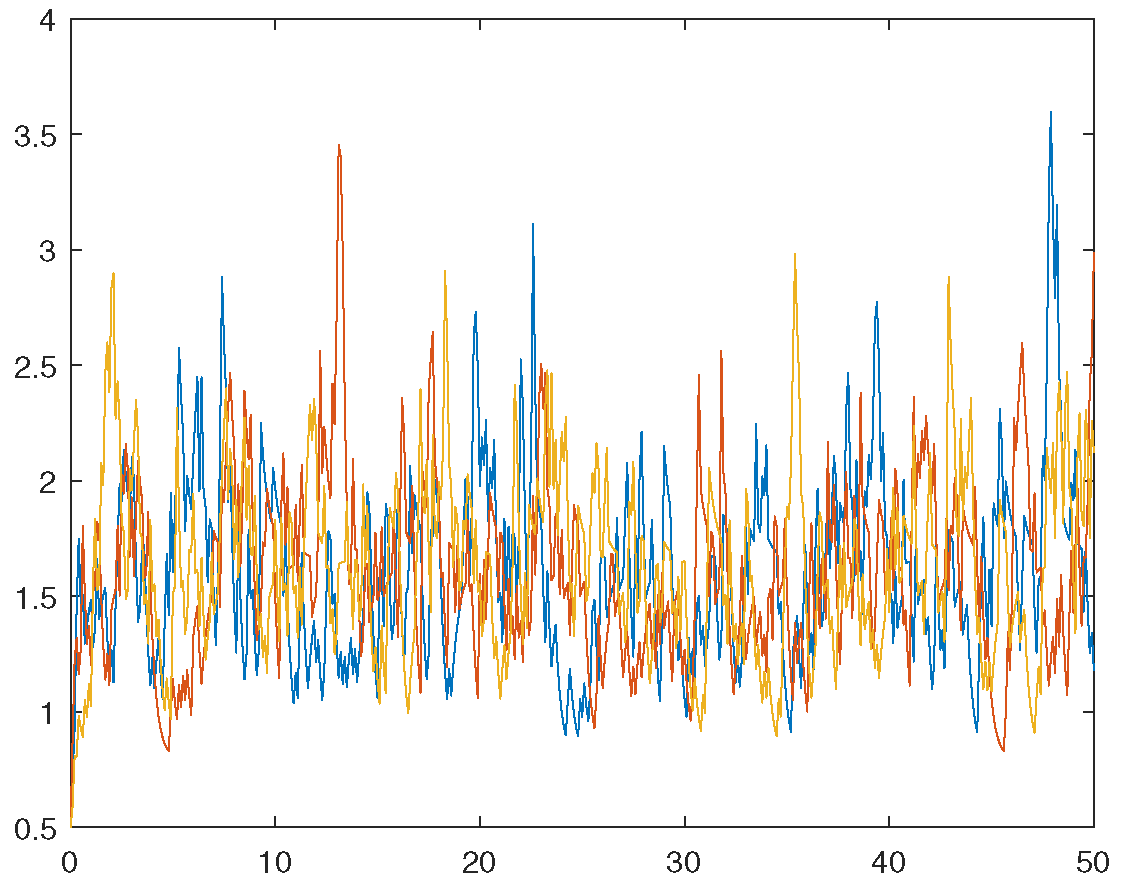
6. Numerical Simulation

In this section, we will perform some numerical simulations to visualize and verify our theoretical results. For a concrete CIR model driven by pure jump process, we take Poisson parameter $\lambda =10$, and as for the CIR model itself, we take $k=3,\theta =0.8$, and $ϵ=0.2$. In order to verify the boundedness of $r\left(t\right)$, we take different initial data $r_0=0.5$ and $r_0=5$; then, we have explicit CIR as follows

$$\begin{array}{c}\hfill \mathrm{d}r\left(t\right)=3(0.8-r\left(t\right))\mathrm{d}t+0.2{\int }_Z\sqrt{r\left(t\right)}\tilde{\eta }(\mathrm{d}t,\mathrm{d}z),r\left(0\right)=r_0.\end{array}$$

(13)

We will use the Euler–Maruyama method to iteration [22], in which the time interval $[0,T]=[0,50]$ and step length $dt={10}^{-1}$. Firstly, we present three sample paths of the solution $r\left(t\right)$ to verify the boundedness of $r\left(t\right)$ in time. Hence, we take the initial data $r_0=0.5$ in Figure 1 and $r_0=5$ in Figure 2, respectively.

Figure 1. Sample paths with $r_0=0.5$.

Figure 2. Sample paths with $r_0=5$.

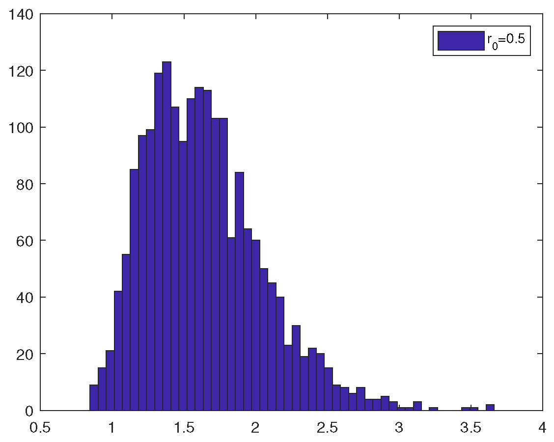
Remark 1.

In Figure 1 and Figure 2, we show sample paths at random, and they undergo great ups and downs, which shows the influence of the Poisson process on the properties of the equation solution well. Meanwhile, the trend of the trajectory shows the effect of the item, $k(\theta -r)$, on the solution, which makes its distribution concentrated as is supposed. Furthermore, the phenomenon verifies our discussion about the boundedness of the solution $r\left(t\right)$ quite well.

In order to show the statistical characteristics to verify the ergodicity of (13), similarly, we take two different initial data $r_0=0.5$ and $r_0=5$ and calculate and count the data of 1000 sample paths. Moreover, the statistical characteristics with different initial data are as follows. In Figure 3 and Figure 4, the values of the 1000 trajectories at the final moment show a tendency to concentrate, which explains the invariant measure numerically.

Figure 3. Empirical density with $r_0=0.5$.

Figure 4. Empirical density with $r_0=5$.