Hierarchical Multi-Scale Decomposition and Deep Learning Ensemble Framework for Enhanced Carbon Emission Prediction

Abstract

Carbon emission prediction is critical for climate change mitigation across industrial, transportation, and urban sectors. Traditional statistical and machine learning methods struggle to capture complex multi-scale temporal patterns and long-range dependencies in emission data. This paper proposes a hierarchical multi-scale decomposition and deep learning ensemble framework that addresses these limitations. We integrate complete ensemble empirical mode decomposition with adaptive noise (CEEMDAN) to decompose carbon emission time series into intrinsic mode functions (IMFs) capturing different frequency bands. Each IMF is processed through a hybrid convolutional neural network (CNN)–Transformer architecture: CNNs extract local features and transformers model long-range dependencies via multi-head attention. An adaptive ensemble mechanism dynamically weights component predictions based on stability and performance metrics. Experiments on four real-world datasets (133,225 observations) demonstrate that our CEEMDAN–CNN–Transformer framework outperforms 12 state-of-the-art methods, achieving a 13.3% reduction in root mean square error (RMSE) to 0.117, 12.7% improvement in mean absolute error (MAE) to 0.088, and 13.0% improvement in continuous ranked probability score (CRPS) to 0.060. The proposed framework not only improves predictive accuracy, but also enhances interpretability by revealing emission patterns across multiple temporal scales, supporting both operational and strategic carbon management decisions.

1. Introduction

Accurate carbon emission prediction has become increasingly critical across numerous domains, including energy production, industrial manufacturing, transportation, urban planning, and environmental policy development [1].In these fields, forecasting errors can lead to substantial consequences, resulting in misallocated resources, ineffective mitigation strategies, and potentially harmful policy decisions [2,3]. The ability to predict future emission values with high precision directly impacts the effectiveness of carbon reduction initiatives, climate action plans, and ultimately, the sustainability of both business operations and public environmental management [4,5]. Despite significant advancements in computational capabilities and algorithmic innovations, carbon emission prediction remains challenging due to the complex nature of temporal dependencies [6], non-linearity, and the presence of both deterministic and stochastic components in real-world emission data [7].

Carbon emission prediction has evolved significantly over the past decade, with researchers progressively moving from traditional statistical methods to sophisticated deep learning frameworks.

Table 1. Comprehensive comparison of carbon emission prediction approaches.

Category	Method	Key Contribution	Limitations
Traditional Decomposition [8]	CEEMDAN-LSTM	Novel secondary decomposition for short-term carbon emission prediction with LSTM network	Single decomposition method, limited to short-term forecasting
Hybrid Deep Learning [9]	LSTM-CNN with Spatial Weights	Coupling LSTM and CNN for accurate provincial carbon emission prediction	Spatial weighting limited to provincial scale, lacks multi-temporal analysis
Multi-scale Decomposition [10]	CEEMDAN-PE-LSTM	Carbon price hybrid model with data multi-scale decomposition and machine learning	Focused on price rather than emission quantity, limited temporal scales
Ensemble Learning [11]	Secondary Decomposition + Stacking	Multi-step carbon emission prediction with secondary decomposition and ensemble strategy	Computational complexity high, ensemble weights not adaptive
Attention Mechanism [12]	ATT-CNN-LSTM	Carbon emission prediction in Zhejiang province using attention-enhanced CNN-LSTM	Attention mechanism complexity, limited to single province
Advanced Decomposition [13]	LSTM–Random Forest Ensemble	High-precision electric carbon factor prediction using deep learning and ensemble learning	Focused on electric carbon factors, not comprehensive emissions
Spatiotemporal Modeling [14]	Hybrid Deep Learning Framework	Spatiotemporal carbon emission prediction considering temporal and spatial correlations	Limited to building-scale emissions, scalability concerns
Reinforcement Learning [15]	Model Matching + Reinforcement Learning	Novel carbon price forecasting with adaptive decomposition and RL ensemble strategy	Complex parameter tuning, primarily for price prediction
Multi-objective Optimization [16]	GWO-XGBOOST-CEEMDAN	Carbon price prediction with decomposition and extreme gradient boosting optimization	Limited to price forecasting, single optimization objective
Explainable AI [17]	Encoder–Decoder with Attention	Robust multi-scale time-series prediction for building carbon emissions with explainable deep learning	Building-specific application, limited transferability

provides a comprehensive comparison of the current carbon emission prediction approaches, highlighting the evolution of methodologies and identifying critical research gaps that our proposed framework addresses.

As shown in Table 1, existing carbon emission prediction methods can be categorized into several main approaches: traditional decomposition methods, hybrid deep learning models, multi-scale decomposition techniques, ensemble learning strategies, attention mechanisms, and spatiotemporal modeling frameworks. While these methods have achieved notable improvements in prediction accuracy, several critical limitations persist.

The evolution of technical frameworks reveals three primary research gaps that limit current carbon emission prediction capabilities. First, existing decomposition techniques typically employ single or dual decomposition methods, failing to capture the full spectrum of temporal patterns inherent in carbon emission data. While CEEMDAN has shown superior performance over traditional EMD and EEMD methods, its integration with advanced deep learning architectures remains underexplored. Second, current hybrid deep learning approaches predominantly focus on CNN-LSTM combination, with limited investigation of CNN–Transformer architectures for carbon emission prediction. The self-attention mechanism in transformers offers significant potential for capturing long-range dependencies in emission patterns, yet this capability remains largely untapped in the carbon emission forecasting domain. Third, ensemble learning strategies in existing studies rely primarily on static weighting mechanisms or simple stacking approaches. The absence of adaptive ensemble frameworks that dynamically adjust component weights based on both model performance and stability characteristics represents a significant limitation in current methodologies.

Traditional statistical approaches to carbon emission forecasting have relied predominantly on parametric models that assume specific underlying data structures. Methods such as Autoregressive Integrated Moving Average (ARIMA) [18], exponential smoothing [19], and state-space models [20] have established robust frameworks for capturing linear dependencies and seasonal patterns in emission data. While these approaches offer strong theoretical foundations and interpretability, they exhibit significant limitations when confronted with complex non-linear relationships, high-dimensional data, or irregular temporal patterns that characterize carbon emissions [21,22]. Furthermore, these methods often require extensive domain expertise for proper specification and struggle to adapt to evolving emission characteristics without manual intervention [23].

Machine learning approaches constitute a significant advancement in carbon emission forecasting capabilities. Ensemble methods such as Random Forests [24], Gradient Boosting Machines [25], and Support Vector Regression [26] have shown remarkable success in capturing non-linear relationships and handling high-dimensional feature spaces. These methods effectively leverage multiple predictors to reduce variance and mitigate overfitting concerns [27]. Nevertheless, conventional machine learning approaches often treat emission observations as independent instances, failing to adequately model the sequential nature and temporal dependencies inherent in carbon emission data [28]. This fundamental limitation hinders their ability to capture complex sequential patterns, particularly when dealing with long-term dependencies and multi-scale temporal structures in emission trends [29].

Deep learning methodologies have revolutionized the field of carbon emission forecasting by introducing specialized architectures designed to capture intricate temporal patterns. Recurrent neural networks (RNNs) [8], long short-term memory networks (LSTMs) [9], and their variants have demonstrated significant improvements in modeling sequential dependencies in emission data. More recently, attention-based mechanisms [30] and transformer architectures [31] have further enhanced the capacity to capture long-range dependencies while addressing computational efficiency concerns. Despite these advancements, deep learning approaches continue to face challenges related to interpretability [32], extensive data requirements, and computational demands, which can limit their applicability in certain environmental management domains where transparency and efficiency are paramount.

The limitations of existing methods stem from two primary factors. First, conventional feature engineering techniques like lag features and rolling statistics often fail to capture hierarchical temporal patterns in carbon emissions that manifest at different granularities [33]. Second, most approaches treat carbon emission prediction as a pure regression problem without explicitly modeling the underlying spatiotemporal patterns that govern emission behavior. This oversight leads to suboptimal performance when dealing with heterogeneous temporal regimes that require different predictive models for different conditions and scales.

We address these challenges through a novel multi-scale decomposition and deep learning ensemble framework that systematically transforms raw carbon emission data into interpretable components. Our approach builds upon the complete ensemble empirical mode decomposition with adaptive noise (CEEMDAN) technique to decompose carbon emission time series into multiple intrinsic mode functions (IMFs), with each intrinsic mode function (IMF) representing oscillations within specific frequency bands. These decomposed components are then processed through a specialized architecture combining convolutional neural networks (CNNs) for local feature extraction and transformer models for capturing long-range dependencies. This hybrid approach leverages the strengths of both architectures: convolutional neural networks (CNNs) excel at identifying local patterns and reducing feature dimensionality, while transformers effectively model complex dependencies across extended sequences through their multi-head self-attention mechanism. This paper contributes to the field of carbon emission prediction through four key innovations:

• We formalize a multi-scale decomposition framework based on CEEMDAN that captures emission patterns at multiple temporal scales while preserving interpretability.
• We introduce a novel CNN–Transformer hybrid architecture specifically designed for processing decomposed carbon emission data.
• We develop an adaptive ensemble mechanism that optimally combines predictions from individual IMF models based on their empirical performance and stability characteristics.
• We demonstrate through extensive experiments that our approach outperforms existing methods while providing actionable insights into the temporal dynamics of carbon emissions across multiple domains.

The remainder of this paper is structured as follows: Section 2 outlines our proposed approach. Section 3 covers the experimental setup and results. Section 4 discusses implications and future directions, concluding with Section 5.

2. Materials and Methods

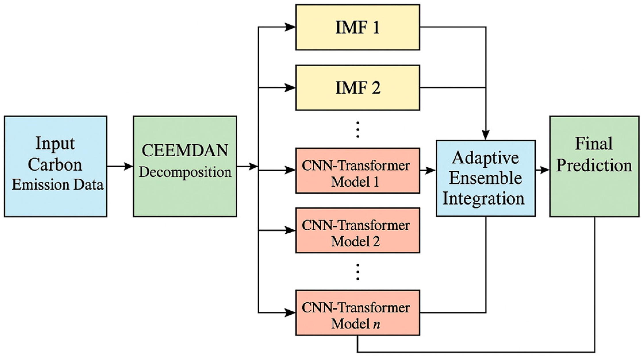
This paper proposes a novel hierarchical multi-scale decomposition and deep learning ensemble framework for enhanced carbon emission prediction. The framework systematically integrates advanced time-series decomposition techniques with specialized neural network architectures to capture complex temporal patterns across multiple scales. Figure 1 depicts the comprehensive architecture of the proposed framework, which consists of four primary components: (1) data collection and preprocessing, (2) multi-scale decomposition using CEEMDAN, (3) component-wise modeling using CNN–Transformer hybrid architectures, and (4) adaptive ensemble integration.

2.1. Data Collection and Preprocessing

Initially, comprehensive data preprocessing is conducted to ensure high-quality inputs for subsequent modeling stages. The raw carbon emission time-series data undergo a systematic preprocessing pipeline designed to address common challenges in temporal data analysis [34]. Then, we implement data cleaning procedures to handle outliers using the modified Z-score method [35], which identifies anomalous emission observations based on the median absolute deviation, providing robustness against extreme values without assumptions about data distribution. Missing values are addressed through a hybrid imputation strategy that employs linear interpolation for short gaps (<3 time steps) and a more sophisticated temporal pattern-based imputation for extended missing segments in the emission records [36].

The carbon emission time-series data are then subjected to normalization using a robust scaler that transforms features based on the interquartile range, thereby minimizing the influence of outliers while preserving the relative relationships between observations. Seasonal adjustment is performed when applicable, with seasonality in carbon emissions detected through both spectral analysis and autocorrelation function examination. For emission data exhibiting strong seasonal components, we apply a seasonal decomposition to isolate the trend, seasonal, and residual components, which are processed separately before recombination in later stages. Temporal alignment is critical when working with multiple emission time series or exogenous variables. We ensure consistent sampling frequency through resampling techniques appropriate to the data characteristics—linear or cubic spline interpolation for upsampling and carefully selected aggregation functions (mean, sum, max, or last value) for downsampling, depending on the specific variable semantics. Additionally, we implement a sliding window approach for feature generation, where window sizes are determined adaptively based on the detected periodicity and autocorrelation structure of each carbon emission time series.

The preprocessed data is then partitioned into training, validation, and test sets using a temporal split strategy that preserves the chronological order of observations. For our experiments, we partition 70% of the data for training, 15% for validation during model development and hyperparameter tuning, and 15% for final testing and performance evaluation. This partitioning ensures that models are evaluated on future emission data, simulating real-world forecasting scenarios while providing sufficient data for robust model training and validation. 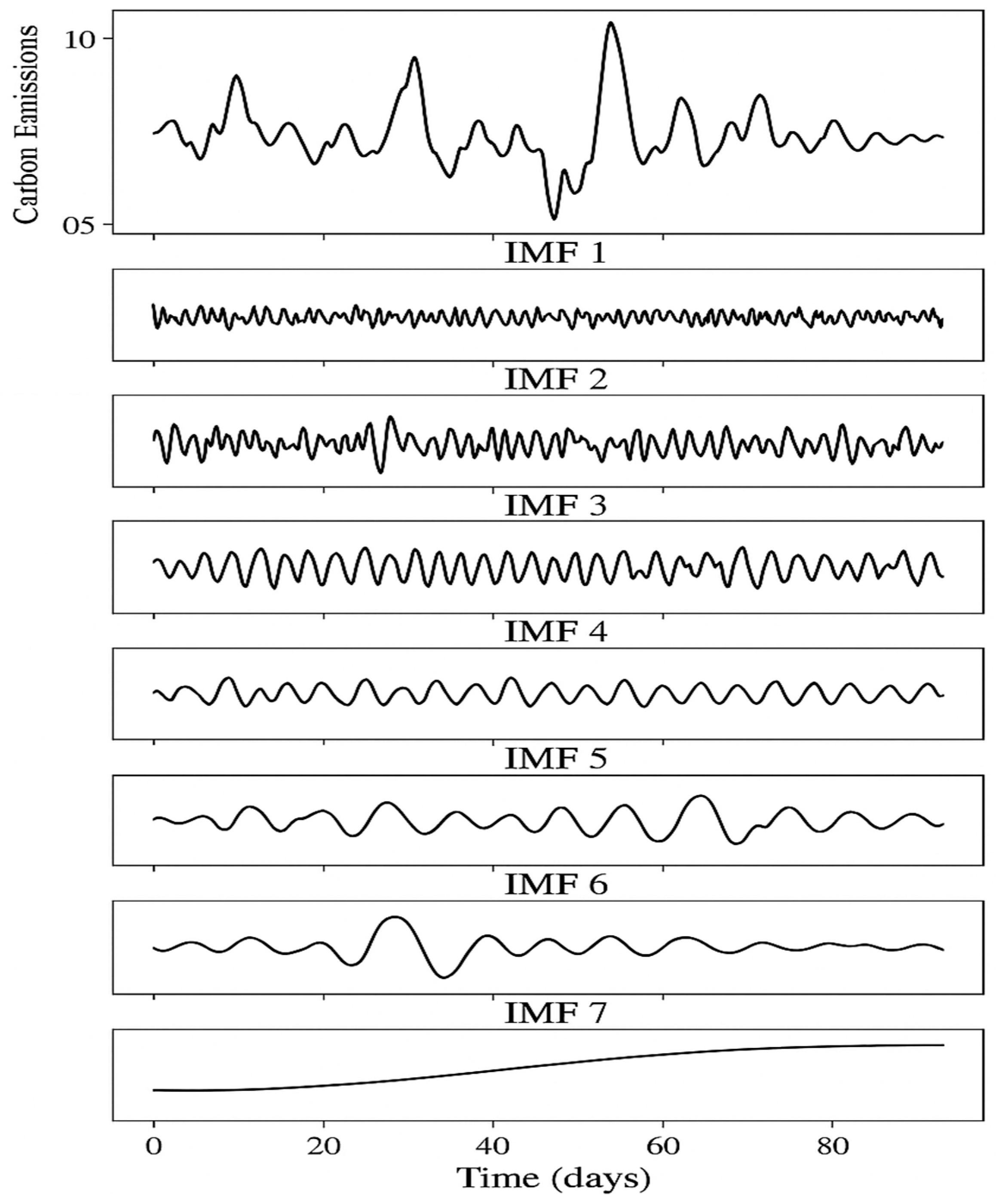Figure 2 illustrates how the CEEMDAN method decomposes a raw carbon emission time series into a collection of IMFs, each corresponding to a distinct frequency band. The higher-order IMFs typically capture fast, high-frequency variations such as daily or random fluctuations, while lower-order IMFs represent more stable, low-frequency components like seasonal trends or long-term patterns. The residual component reflects the overarching trend in emissions. By isolating these components, CEEMDAN enables a more accurate and interpretable modeling of multi-scale temporal behaviors in carbon emissions.

2.2. CEEMDAN for Multi-Scale Decomposition

The selection of CEEMDAN as our primary decomposition method is based on systematic evaluation against alternative techniques for carbon emission time-series analysis. We established four key selection criteria: (1) mode-mixing mitigation capability; (2) noise robustness under typical emission monitoring conditions; (3) computational efficiency for real-time applications; (4) interpretability of decomposed components.

Comparative analysis reveals CEEMDAN’s superiority over alternatives: EMD suffers from significant mode-mixing issues that contaminate frequency separation; EEMD, while addressing mode mixing, requires extensive computational resources; VMD demands the pre-specification of component numbers, limiting adaptability; DWT and SSA show limited effectiveness for non-stationary emission patterns. CEEMDAN uniquely combines excellent mode-mixing mitigation with adaptive noise handling, producing stable, interpretable decompositions without requiring predetermined parameters.

The core focus of our approach is the application of CEEMDAN for the multi-scale temporal analysis of carbon emission data [37]. CEEMDAN represents a significant advancement over traditional decomposition methods by adaptively decomposing non-linear and non-stationary emission time series into a finite set of IMFs that capture oscillations at different frequency bands. This technique addresses the mode-mixing problem found in the original empirical mode decomposition (EMD) method [38] and reduces the computational complexity of ensemble EMD (EEMD) [39] while maintaining noise separation properties.

For a given carbon emission time series x(t), CEEMDAN works by iteratively extracting IMFs through a sifting process. Initially, we add white noise to the original signal and decompose it using EMD.

$$x^{\left(i\right)}\left(t\right)=x\left(t\right)+\beta w^{\left(i\right)}\left(t\right),$$

(1)

where $w^{\left(i\right)}\left(t\right)$ represents the i-th white noise realization with unit variance and β controls the noise amplitude. The CEEMDAN algorithm then computes the first IMF as the average of the first IMFs from multiple noise-added realizations.

$${IMF}_1=\left({\displaystyle \frac{1}{I}}\right)·{\sum }_{i=1}^I{{IMF}_1}^{\left(i\right)}.$$

(2)

For subsequent IMFs, CEEMDAN applies EMD to the residual signal with new noise realizations, ensuring that each IMF captures a distinct frequency band of the original emission signal. This approach helps isolate specific emission patterns, such as daily fluctuations, weekly cycles, seasonal variations, and long-term trends, into separate components that can be modeled individually.

The number of IMFs generated by CEEMDAN is logarithmically related to the data length, typically yielding 8–12 components for our carbon emission datasets. Each IMF represents a different temporal scale, with the first IMFs capturing high-frequency fluctuations (often corresponding to noise or rapid emission changes) and subsequent IMFs revealing progressively lower-frequency oscillations (weekly patterns, seasonal trends, etc.). The final residual component represents the overall trend in carbon emissions.

The CEEMDAN decomposition offers several advantages for carbon emission analysis. First, it allows for the adaptive extraction of emission patterns without imposing predefined frequency bands, making it suitable for the complex and evolving nature of emission data. Second, it separates the multi-scale components of the signal while maintaining their temporal alignment, facilitating the identification of scale-specific relationships between emissions and driving factors. Third, by isolating different temporal regimes, it enables more specialized modeling approaches for each component, potentially improving overall prediction accuracy.

The CEEMDAN Multi-Scale Decomposition algorithm implements a systematic approach to decompose carbon emission time series into intrinsic mode functions (IMFs) representing distinct frequency bands. The algorithm initiates by setting the original carbon emission sequence as the initial residual and establishing an IMF counter. Subsequently, it proceeds through an iterative mode extraction process, wherein white noise ensembles are generated and added to the residual with controlled amplitude. For each noise-added realization, the first mode is extracted via the EMD sifting process. The ensemble average of these extractions constitutes the current IMF component, which is then subtracted from the residual to prepare for the next iteration. This process continues until a predefined stopping criterion is satisfied, typically when the residual becomes monotonic or falls below a significance threshold. The algorithm’s sophistication lies in its adaptive noise integration mechanism, which mitigates mode mixing while preserving the temporal integrity of the emission patterns across different scales. For details refer to Algorithm 1 below.

Algorithm 1: CEEMDAN Multi-Scale Decomposition

Require: Carbon emission time series x(t) = {x1, x2, …, xt},

number of noise realizations I, noise amplitude β

Ensure: IMFs = {IMF1, IMF2, …, IMFn}, residual r

Step 1: Initialize Decomposition

1: Set residual r(0) ← x(t)

2: Initialize IMF counter j ← 1

3: Initialize IMF list ← []

Step 2: Iterative Mode Extraction

4: while Stopping Criterion(r(j−1)) not satisfied do

5:  Generate noise ensemble W = {w(1), w(2), …, w(I)}

6:  for i = 1 to I do

7:      Add noise to residual: $x~$(i) ← r(j−1) + β × Eⱼ(w(i))

8:      Extract first mode: m(i) ← EMD_FirstMode($x~$(i))

9:  end for

10:  Compute ensemble average: IMFⱼ ← $\left({\displaystyle \frac{1}{I}}\right)·{\sum }_{i=1}^I{M}^{\left(i\right)}$

11:  Update residual: r(j) ← r(j−1) − IMFⱼ

12: Store IMF: IMF list.append(IMFⱼ)

13:  j ← j + 1

14: end while

Step 3: Finalize Decomposition

15: residual ← r(j−1)

16: return IMF list, residual

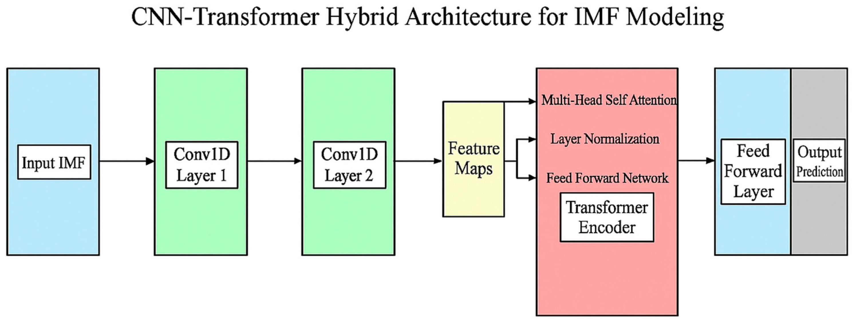
2.3. CNN–Transformer Hybrid Architecture

Our proposed approach employs a hybrid CNN–Transformer architecture to effectively model the multi-scale temporal patterns in decomposed carbon emission data [40]. This architecture leverages the complementary strengths of convolutional neural networks for local feature extraction [41] and transformer models for capturing long-range dependencies [42].

For each IMF component extracted through CEEMDAN, we design a specialized model that first applies one-dimensional convolutional layers to identify local patterns and reduce dimensionality [43]. The CNN component consists of multiple convolutional blocks, each comprising a 1D convolutional layer followed by batch normalization, ReLU activation, and dropout for regularization. The convolutional layers employ multiple filter sizes to capture patterns at different scales, with the number of filters increasing progressively in deeper layers to enhance representational capacity. This approach allows the model to effectively extract relevant features from each IMF while filtering out noise components.

The output features from the CNN component are then fed into a transformer encoder to model complex temporal dependencies. The transformer architecture, based on the self-attention mechanism, computes attention weights that represent the relevance of each time step to every other time step in the sequence.

$$Attention\left(Q,K,V\right)=softmax\left({\displaystyle \frac{Q{K}^T}{\sqrt{d_{\mathrm{k}}}}}\right)V,$$

(3)

where Q, K, and V represent the query, key, and value matrices derived from linear transformations of the input, and $d_k$ is the dimension of the key vectors. The multi-head attention mechanism performs this attention computation multiple times in parallel, allowing the model to attend to information from different representation subspaces.

$$MultiHead\left(Q,K,V\right)=Concat\left({head}_1,{head}_2,\dots ,{head}_{\mathrm{h}}\right)W^O,$$

(4)

where ${Head}_i=Attention({QW}_{i^Q},{KW}_{i^K},{VW}_{i^V})$. This multi-head attention approach enables the model to simultaneously attend to different temporal patterns present in carbon emission data, such as daily cycles, weekly patterns, and longer-term trends.

The transformer encoder stacks multiple layers of multi-head self-attention followed by position-wise feed-forward networks, layer normalization, and residual connections. This deep architecture allows for hierarchical representation learning of temporal dependencies in carbon emissions at multiple levels of abstraction. To preserve temporal information in the absence of recurrence, we incorporate positional encodings that inject information about the relative or absolute position of time steps in the sequence. The output from the transformer encoder is then processed through a final feed-forward layer to generate predictions for each IMF component. Figure 3 illustrates our CNN–Transformer hybrid architecture for processing individual IMF components.

2.4. Multi-Component Ensemble Integration

Our carbon emission prediction framework employs a multi-component ensemble approach that integrates predictions from individual IMF models to generate the final forecast [44]. After obtaining separate predictions for each IMF component, we combine them through an adaptive weighting mechanism that considers both the inherent characteristics of each component and their empirical prediction performance [45].

The weighting strategy assigns importance to each IMF component based on two primary factors: (1) the stability of the component, measured through its signal-to-noise ratio and consistency across different time periods, and (2) the recent prediction accuracy of the corresponding model. For a given carbon emission time series decomposed into n IMF components plus a residual, the final prediction is computed as

$${\widehat{y}}_t={\sum }_{i=1}^{n+1}{w}_{i,t}· {\widehat{y}}_{i,t},$$

(5)

where ${\widehat{y}}_{i,t}$ is the prediction for the i-th component at time t, and $w_{i,t}$ is the corresponding weight. The weights are determined by

$$w_{i,t}={\displaystyle \frac{\mathit{exp}\left({\gamma }_1{p}_{i,t}+{\gamma }_2{s}_{i,t}\right)}{{\sum }_{i=1}^{n+1}\mathit{exp}({\gamma }_1{p}_{j,t}+{\gamma }_2{s}_{j,t})}},$$

(6)

where $p_{i,t}$ represents the recent performance score (inverse of mean squared error over a sliding window), $s_{i,t}$ is the stability score of the i-th component, and γ₁ and γ₂ are hyperparameters that control the relative importance of performance and stability, respectively.

The stability score $s_{i,t}$ for each IMF is calculated based on its contribution to the original signal’s variance and its autocorrelation properties, reflecting the regularity and predictability of the component. Higher weights are assigned to components that demonstrate consistent patterns and better predictive performance, allowing the ensemble to adapt to changing emission dynamics.

Additionally, we implement a hierarchical ensemble strategy that first combines predictions within frequency bands (grouping similar-frequency IMFs) before integrating across all scales. This approach acknowledges that certain emission factors may influence specific frequency bands differently, enhancing the model’s ability to capture multi-scale dependencies.

Figure 4 shows our prediction framework. The Adaptive Ensemble Integration Framework orchestrates the synthesis of predictions from multiple component models trained on different IMF components to generate comprehensive carbon emission forecasts. The algorithm commences with a uniform initialization of ensemble weights and subsequently computes dual evaluation metrics for each component: performance scores derived from validation accuracy and stability scores reflecting variance contribution and autocorrelation characteristics. These metrics are then combined through hyperparameters γ₁ and γ₂ to calculate adaptive weights, which undergo normalization to ensure proper probability distribution. The framework’s dynamic adaptation capability is implemented through a sliding window mechanism that evaluates recent prediction errors and adjusts component weights accordingly. This temporal responsiveness enables the ensemble to prioritize components that demonstrate consistent predictive accuracy as emission patterns evolve. The algorithm culminates in the generation of weighted ensemble predictions that effectively leverage the complementary strengths of different temporal scale models, thereby enhancing overall forecast accuracy and robustness across diverse emission scenarios. For details refer to Algorithm 2 below.

Algorithm 2: Adaptive Ensemble Integration Framework

Require: Component models M = {M1, M2,…, Mn₊1}, validation data $X_{val}$,

ensemble parameters γ1, γ2, $windo{w}_{size}$W

Ensure: Ensemble predictions ${\widehat{y}}_{ensemble}$, component weights w

Step 1: Initialize Ensemble Weights

1: $n_{components}$ ← |M|

2: Initialize weights w ← [1/$n_{components}$,…, 1/$n_{components}$]

Step 2: Compute Performance and Stability Scores

3: $performanc{e}_{scores}$ p ← []

4: $stabilit{y}_{scores}$ s ← []

5: for i = 1 to $n_{components}$ do

6:  $prediction{s}_{val}$ ← $Mᵢ.predict\left(X_{val}\right)$

7:  mse ← MSE($prediction{s}_{val}$, $y_{val}$)

8:  pᵢ ← $\exp \left(-mse\right)$

9:  $varianc{e}_{contrib}$ ← Var($prediction{s}_{val}$)/$Var\left(y_{val}\right)$

10:  autocorr ← Auto Correlation($prediction{s}_{val}$, lag = 1)

11:  sᵢ ← ($varianc{e}_{contrib}$ + |autocorr|)/2

12: end for

Step 3: Calculate Adaptive Weights

13: for i = 1 to $n_{components}$ do

14:  score ← γ1 × pᵢ + γ2 × sᵢ

15:  wᵢ ← exp(score)

16: end for

17: Normalize weights: w ← w/sum(w)

Step 4: Generate Ensemble Predictions

18: Initialize predictions matrix P ∈ ℝᵀˣⁿ

19: for i = 1 to $n_{components}$ do

20:  P[:, i] ← $Mᵢ.predict\left(X_{test}\right)$

21: end for

22: $ensembl{e}_{predictions}$ ← []

23: for t = 1 to T do

24:  if t ≥ W then

25:     for i = 1 to $n_{components}$ do

26:       $recen{t}_{error}$ ← $MSE\left(P\left[t-W:t, i\right], y\left[t-W:t\right]\right)$

27:       $performanc{e}_{factor}$ ← exp(−λ × $recen{t}_{error}$)

28:     wᵢ,t ← wᵢ × $performanc{e}_{factor}$

29:     end for

30:     Normalize: wₜ ← wₜ/sum(wₜ)

31:  else

32:      wₜ ← w

33:  end if

34:

35:  ŷₜ ← ∑ᵢ₌1ⁿ wᵢ,ₜ × P[t, i]

36:   $ensembl{e}_{predictions}.append\left(\widehat{y}t\right)$

37: end for

38: return $ensembl{e}_{predictions}$, w

2.5. Model Training and Optimization

Our training process for the multi-component ensemble system involves a sophisticated staged approach designed to ensure the optimal performance of each component while preventing information leakage [46]. The approach begins with the CEEMDAN decomposition on the training data to extract IMFs, followed by specialized training for each component using tailored architectural configurations.

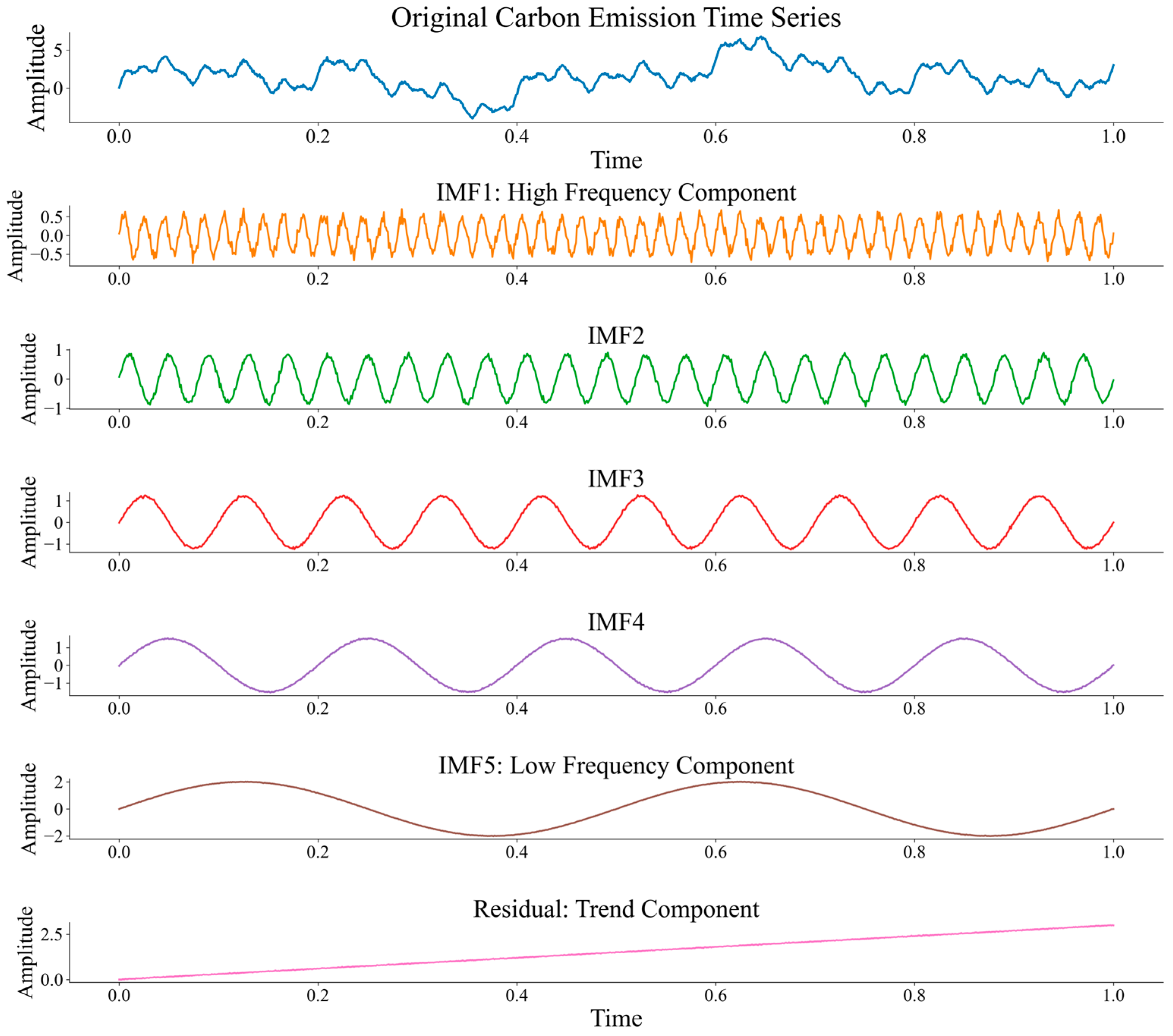
Figure 5 displays the CEEMDAN decomposition process, illustrating how the original carbon emission time series is separated into IMFs with distinct frequency characteristics and a residual trend component. This decomposition forms the foundation of our multi-scale modeling approach.

2.5.1. Optimization Strategy

For each CNN–Transformer model, we employ the Adam optimizer (Adaptive Moment Estimation) with a carefully designed learning rate schedule [47]. The Adam optimizer has been widely adopted in deep learning applications due to its ability to adaptively adjust learning rates for different parameters based on gradient history [48]. The update rule for Adam can be formulated as

$$m_t={\beta }_1{m}_{t-1}+\left(1-{\beta }_1\right)g_t,$$

(7)

$$v_t={\beta }_2{v}_{t-1}+\left(1-{\beta }_2\right){g_t}^2,$$

(8)

$${\widehat{m}}_t={\displaystyle \frac{m_t}{1-{{\beta }_1}^t}},$$

(9)

$${\widehat{v}}_t={\displaystyle \frac{v_t}{1-{{\beta }_2}^t}},$$

(10)

$${\theta }_t={\theta }_{t-1}-\alpha {\displaystyle \frac{{\widehat{m}}_t}{\sqrt{{\widehat{v}}_t}+ϵ}},$$

(11)

where $m_t$ and $v_t$ are the first and second moment estimates, ${\widehat{m}}_t$ and ${\widehat{v}}_t$ are their bias-corrected versions, $g_t$ is the gradient at time step t, ${\theta }_t$ represents the model parameters, $\alpha$ is the learning rate, and ${\beta }_1$, ${\beta }_2$, and $ϵ$ are hyperparameters with default values of 0.9, 0.999, and ${10}^{-8}$, respectively.

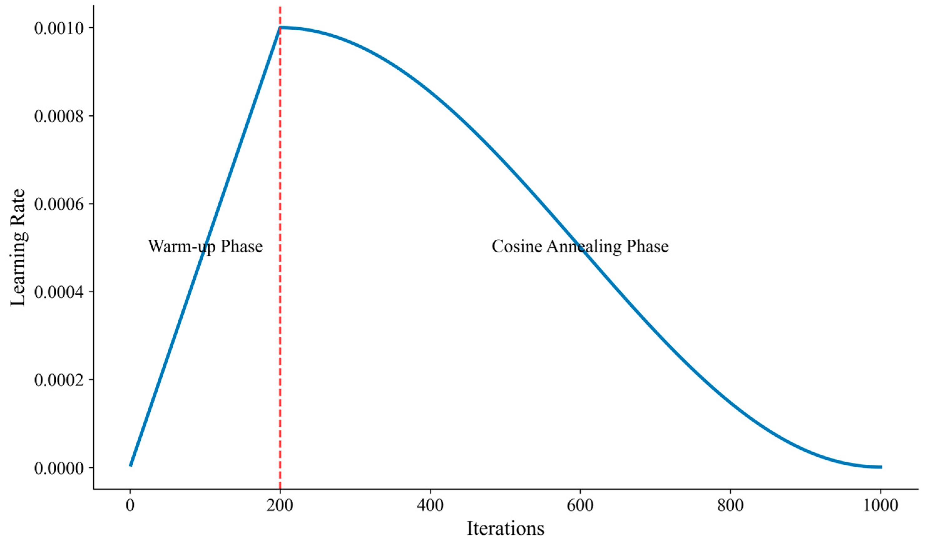
Our implementation incorporates a learning rate scheduler with a warm-up phase followed by cosine annealing. During the warm-up phase, the learning rate gradually increases from an initial small value ${\alpha }_{init}$ to a predefined maximum ${\alpha }_{max}$ over $N_{warmup}$ iterations:

$${\alpha }_t={\alpha }_{\mathrm{i}\mathrm{n}\mathrm{i}\mathrm{t}}+\left({\alpha }_{\mathrm{m}\mathrm{a}\mathrm{x}}-{\alpha }_{\mathrm{i}\mathrm{n}\mathrm{i}\mathrm{t}}\right)\times {\displaystyle \frac{t}{N_{\mathrm{w}\mathrm{a}\mathrm{r}\mathrm{m}\mathrm{u}\mathrm{p}}}}, for t\le N_{\mathrm{w}\mathrm{a}\mathrm{r}\mathrm{m}\mathrm{u}\mathrm{p}}.$$

(12)

This warm-up phase stabilizes the early stages of training, particularly for the transformer component, which can be sensitive to learning rate settings. Following the warm-up phase, we apply cosine annealing to gradually reduce the learning rate according to

$${\alpha }_t={\alpha }_{\mathrm{m}\mathrm{i}\mathrm{n}}+{\displaystyle \frac{1}{2}}\left({\alpha }_{\mathrm{m}\mathrm{a}\mathrm{x}}-{\alpha }_{\mathrm{i}\mathrm{n}\mathrm{i}\mathrm{t}}\right)(1+\mathrm{c}\mathrm{o}\mathrm{s}\left({\displaystyle \frac{t-N_{\mathrm{w}\mathrm{a}\mathrm{r}\mathrm{m}\mathrm{u}\mathrm{p}}}{{N_{\mathrm{t}\mathrm{o}\mathrm{t}\mathrm{a}\mathrm{l}}-N}_{\mathrm{w}\mathrm{a}\mathrm{r}\mathrm{m}\mathrm{u}\mathrm{p}}}}\pi \right), for t\ge N_{\mathrm{w}\mathrm{a}\mathrm{r}\mathrm{m}\mathrm{u}\mathrm{p}},$$

(13)

where $N_{total}$ is the total number of training iterations and ${\alpha }_{min}$ is the minimum learning rate. This schedule enables fine-grained parameter updates as training progresses, helping the model converge to better solutions by effectively exploring the parameter space. Figure 6 illustrates our learning rate scheduling strategy, showing both the warm-up phase and the cosine annealing phase used during model training.

To prevent exploding gradients, which are particularly problematic for deep transformer networks, we implement gradient clipping by constraining the norm of the gradient vector

$$g_t^{\prime }=g_t\times \min \left(1,{\displaystyle \frac{\lambda }{{\left|\left|g_t\right|\right|}_2}}\right),$$

(14)

where λ is the gradient clipping threshold and ${\left|\left|g_t\right|\right|}_2$ is the l₂ norm of the gradient. This technique stabilizes training by preventing excessively large parameter updates that could derail the optimization process.

2.5.2. Regularization Techniques

To mitigate overfitting, we implement several regularization strategies throughout our framework. For the CNN components, we apply dropout with probability $p_{CNN}$ after each convolutional block.

$$h_i^{\prime }=\left\{\begin{array}{cc}{\displaystyle \frac{h_i}{1-p_{\mathrm{C}\mathrm{N}\mathrm{N}}}}& \mathrm{w}\mathrm{i}\mathrm{t}\mathrm{h} \mathrm{p}\mathrm{r}\mathrm{o}\mathrm{b}\mathrm{a}\mathrm{b}\mathrm{i}\mathrm{l}\mathrm{i}\mathrm{t}\mathrm{y} {1-p}_{\mathrm{C}\mathrm{N}\mathrm{N}}\\ 0& \mathrm{w}\mathrm{i}\mathrm{t}\mathrm{h} \mathrm{p}\mathrm{r}\mathrm{o}\mathrm{b}\mathrm{a}\mathrm{b}\mathrm{i}\mathrm{l}\mathrm{i}\mathrm{t}\mathrm{y} p_{\mathrm{C}\mathrm{N}\mathrm{N}}\end{array}\right.,$$

(15)

where $h_i$ and $h_i^{\prime }$ represent the activation before and after dropout, respectively. The scaling factor ${\displaystyle \frac{1}{1-p_{CNN}}}$ ensures that the expected sum of the activations remains unchanged during training.

For the transformer components, we employ dropout both in the attention mechanism and after feed-forward layers, along with attention dropout, which randomly masks elements in the attention matrix.

$$A_{\mathrm{m}\mathrm{a}\mathrm{s}\mathrm{k}\mathrm{e}\mathrm{d}}(i,j)=\left\{\begin{array}{cc}{\displaystyle \frac{A(i,j)}{1-p_{\mathrm{a}\mathrm{t}\mathrm{t}\mathrm{n}}}}& \mathrm{w}\mathrm{i}\mathrm{t}\mathrm{h} \mathrm{p}\mathrm{r}\mathrm{o}\mathrm{b}\mathrm{a}\mathrm{b}\mathrm{i}\mathrm{l}\mathrm{i}\mathrm{t}\mathrm{y} 1-p_{\mathrm{a}\mathrm{t}\mathrm{t}\mathrm{n}}\\ 0& \mathrm{w}\mathrm{i}\mathrm{t}\mathrm{h} \mathrm{p}\mathrm{r}\mathrm{o}\mathrm{b}\mathrm{a}\mathrm{b}\mathrm{i}\mathrm{l}\mathrm{i}\mathrm{t}\mathrm{y} p_{\mathrm{a}\mathrm{t}\mathrm{t}\mathrm{n}}\end{array}\right.,$$

(16)

where A(i, j) represents the attention weight between positions i and j.

Additionally, we incorporate weight decay regularization in the optimizer, which penalizes the l₂ norm of the model parameters.

$$L_{\mathrm{t}\mathrm{o}\mathrm{t}\mathrm{a}\mathrm{l}}=L_{\mathrm{d}\mathrm{a}\mathrm{t}\mathrm{a}}+{\lambda }_{\mathrm{d}\mathrm{e}\mathrm{c}\mathrm{a}\mathrm{y}}\sum _i{\theta }_i^2,$$

(17)

where $L_{\mathrm{d}\mathrm{a}\mathrm{t}\mathrm{a}}$ is the primary loss function, ${\lambda }_{\mathrm{d}\mathrm{e}\mathrm{c}\mathrm{a}\mathrm{y}}$ is the weight decay coefficient, and θ_i represents the model parameter. This encourages the model to learn simpler patterns and avoid overreliance on specific parameters.

We also implement early stopping based on validation performance with a patience of 20 epochs, halting training when the validation metric fails to improve for this duration. This prevents overfitting by finding the optimal trade-off between underfitting and overfitting. The early stopping criterion can be formulated as

$$\mathrm{S}\mathrm{t}\mathrm{o}\mathrm{p} \mathrm{i}\mathrm{f} M_t<{max}_{t-P\le j<t}{M}_j,$$

(18)

where $M_t$ is the validation metric at epoch t and P is the patience parameter.

2.5.3. Loss Function Design

Our loss function combines mean squared error (MSE) for point prediction accuracy with a custom component that penalizes phase shifts in the predicted signals.

$$L_{\mathrm{t}\mathrm{o}\mathrm{t}\mathrm{a}\mathrm{l}}={\alpha }_{\mathrm{M}\mathrm{S}\mathrm{E}}{L}_{\mathrm{M}\mathrm{S}\mathrm{E}}+{\alpha }_{\mathrm{p}\mathrm{h}\mathrm{a}\mathrm{s}\mathrm{e}}{L}_{\mathrm{p}\mathrm{h}\mathrm{a}\mathrm{s}\mathrm{e}},$$

(19)

where ${\alpha }_{\mathrm{M}\mathrm{S}\mathrm{E}}$ and ${\alpha }_{\mathrm{p}\mathrm{h}\mathrm{a}\mathrm{s}\mathrm{e}}$ are weighting coefficients that balance the two components. The MSE loss is defined as

$$L_{\mathrm{M}\mathrm{S}\mathrm{E}}={\displaystyle \frac{1}{N}}{\sum }_{i=1}^N(y_i-{\widehat{y}}_i{)}^2,$$

(20)

where $y_i$ and ${\widehat{y}}_i$ are the true and predicted values, respectively, and N is the number of samples.

The phase loss component, which is particularly important for capturing the correct timing of emission patterns, is calculated using the cross-correlation between the predicted and actual signals:

$$L_{\mathrm{p}\mathrm{h}\mathrm{a}\mathrm{s}\mathrm{e}}=1-{max}_{\tau }{\displaystyle \frac{R_{y\widehat{y}}\left(\tau \right)}{\sqrt{R_{yy}\left(0\right)·R_{\widehat{y}\widehat{y}}\left(0\right)}}},$$

(21)

where $R_{y\widehat{y}}\left(\tau \right)$ is the cross-correlation function between y and $\widehat{y}$ at lag τ, and $R_{yy}\left(0\right)$ and $R_{\widehat{y}\widehat{y}}\left(0\right)$ are the autocorrelations at zero lag. This loss term ensures that the predicted signals maintain the correct temporal alignment with the actual emission patterns.

2.5.4. Hyperparameter Optimization

Hyperparameter optimization is conducted using Bayesian optimization with a Gaussian Process prior. This approach models the objective function (validation performance) as a sample from a Gaussian process and selects hyperparameters that maximize the expected improvement

$$EI\left(x\right)=E[\left(f\left(x\right)-f\left(x^{+}\right),0\right],$$

(22)

where x represents a hyperparameter configuration, $f\left(x\right)$ is the objective function value, and $x^{+}$ is the best configuration found so far. The optimization process explores the hyperparameter space systematically while balancing exploration and exploitation.

The hyperparameter search space includes learning rates α ∊ [10⁻⁵, 10⁻², dropout rates p ∊ [0.1, 0.5], convolutional filter sizes f ∊ {3, 5, 7}, number of attention heads h ∊ {4, 8, 16}, and ensemble weighting parameters γ₁, γ₂ ∊ [0.1, 5.0]. We employ a composite optimization objective that combines prediction accuracy (weighted RMSE across multiple forecast horizons) and prediction interval quality (average continuous ranked probability score).

$$Obj=\beta ·wRMSE+\left(1-\beta \right)CRPS,$$

(23)

where $\beta$ is a weighting parameter typically set to 0.7 based on empirical performance.

2.5.5. Ensemble Training Strategy

For training the ensemble weights, we use a hold-out portion of the validation set to determine the optimal combination of component predictions. This two-level validation approach ensures that both the individual models and the ensemble integration mechanism are properly tuned without information leakage.

The ensemble weights are adjusted through a gradient-based optimization procedure.

$$w_{i,t+1}=w_{i,t}-\eta {\displaystyle \frac{\partial L}{\partial w_{i,t}}},$$

(24)

where η is the learning rate for the ensemble weights and L is the ensemble loss function. The final ensemble weights are normalized to sum to 1 using a softmax function to ensure proper probability distribution.

$$w_i={\displaystyle \frac{\mathrm{e}\mathrm{x}\mathrm{p}\left(z_i\right)}{{\sum }_j^{n+1}\mathrm{e}\mathrm{x}\mathrm{p}\left(z_j\right)}},$$

(25)

where $z_i$ represents the unnormalized weight for component i.

To enhance the robustness of our ensemble approach, we incorporate a moving window mechanism that dynamically adjusts component weights based on recent performance.

$$p_{i,t}=exp\left(-\lambda {\sum }_{j=t-W}^{t-1}{(y_j-{\widehat{y}}_{i,j})}^2\right),$$

(26)

where $p_{i,t}$ is the performance score for component i at time t, W is the window size, and λ is a scaling parameter.

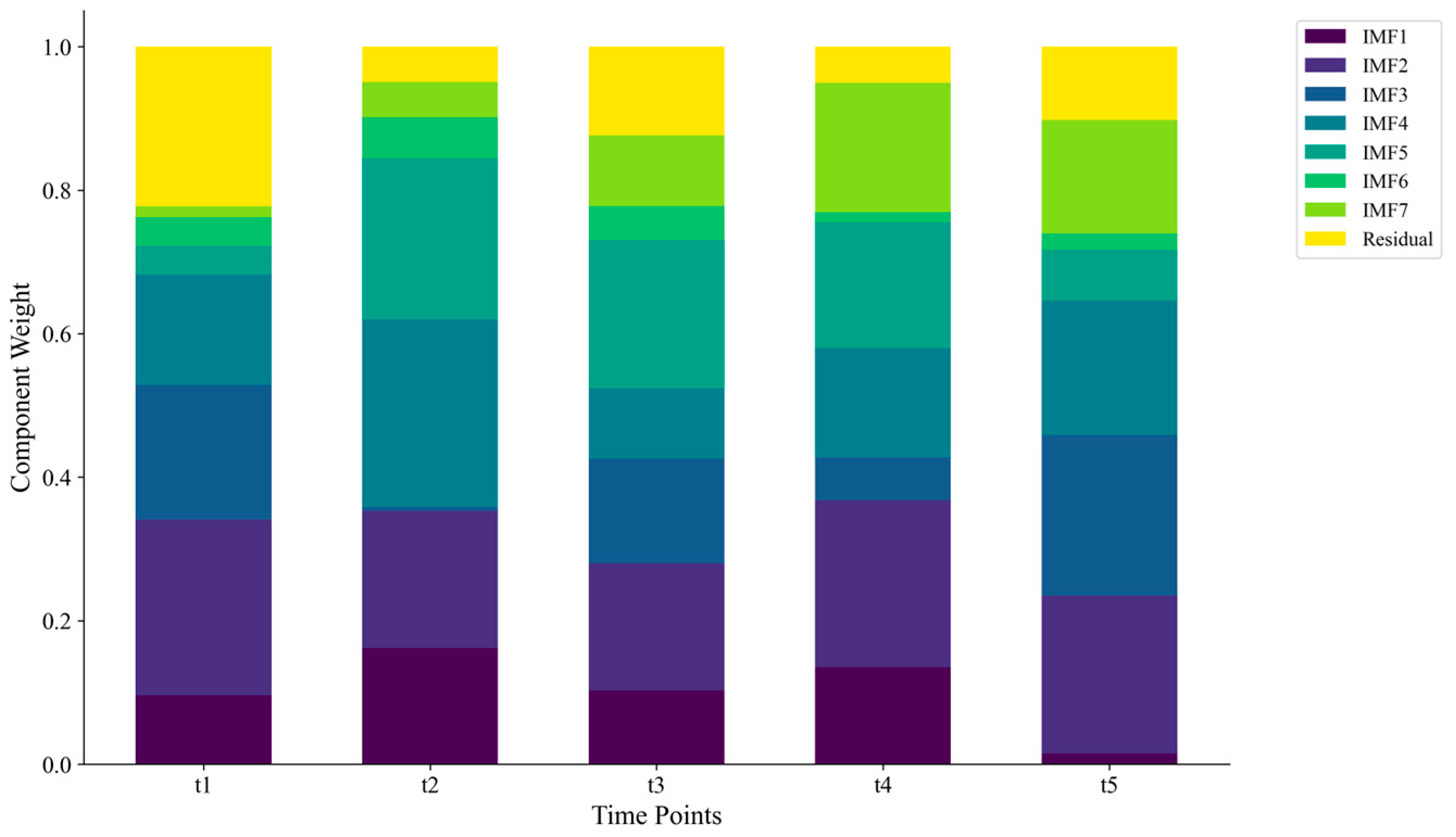
Figure 7 demonstrates the adaptive nature of our ensemble approach, showing how component weights evolve across different time points to emphasize the most relevant IMF components as emission patterns change. This adaptive weighting mechanism allows the ensemble to respond to changing emission dynamics and prioritize components that demonstrate consistent predictive accuracy.

The CNN–Transformer hybrid architecture and training algorithm delineate the construction and optimization of a sophisticated neural network tailored for multi-scale carbon emission modeling. The algorithm is structured in four principal phases: architecture initialization, CNN component development, transformer component integration, and model training optimization. The CNN component is constructed through the iterative addition of convolutional layers with batch normalization, ReLU activation, and dropout regularization, configured with progressive filter sizes to capture hierarchical local patterns in emission data. Subsequently, the transformer component is integrated, commencing with positional encoding followed by multiple transformer layers incorporating multi-head attention mechanisms and feed-forward networks with residual connections. The training phase employs the Adam optimizer with a meticulously designed warm-up cosine annealing learning rate schedule, gradient norm clipping for stabilization, and comprehensive regularization strategies, including dropout variations and weight decay. The implementation of early stopping based on validation performance ensures optimal generalization capability. This hybrid architecture effectively combines the CNN’s capability to extract local features with the transformer’s proficiency in modeling long-range dependencies, creating a robust framework for capturing complex temporal patterns across multiple scales in carbon emission data. For details, refer to Algorithm 3 below.

Algorithm 3: CNN–Transformer Hybrid Architecture and Training

Require: Component data X ∈ ${\mathbb{R}}^{\mathrm{Txd}}$, CNN parameters {$filte{r}_{sizes}, nu{m}_{filters}$},

Transformer parameters {$nu{m}_{heads}, d_{model}$}, training parameters {$lr, epochs$}

Ensure: Trained model $M_{trained}$

Step 1: Model Architecture Construction

1: Initialize model layers ← []

Step 2: CNN Component

2: for layer = 1 to $nu{m}_{cn{n}_{layers}}$ do

3:  Add Conv1D(filters = $nu{m}_{filters}$[layer], $kerne{l}_{size}$ = $filte{r}_{sizes}$[layer])

4:  Add Batch Normalization ()

5:  Add ReLU ()

6:  Add Dropout($p_{cnn}$)

7: end for

Step 3: Transformer Component

8: Add Positional Encoding ($d_{model}$)

9: for layer = 1 to $nu{m}_{transforme{r}_{layers}}$ do

10:  Q, K, V ← LinearProjections(input, $d_{model}$)

11:  attention ← Multi Head Attention (Q, K, V, $nu{m}_{heads}$)

12:  Add LayerNorm(attention + residual)

13:  $f{f}_{output}$ ← Feed Forward ($attentio{n}_{output}$)

14:  Add Layer Norm ($f{f}_{output}$+ residual)

15: end for

16: Add Dense (1)//Output layer

Step 4: Model Training

17: Initialize optimizer ← Adam($lr={\alpha }_{init}$, β1 = 0.9, β2 = 0.999)

18: Initialize scheduler ← WarmupCosineAnnealing(${\alpha }_{max}$, ${\alpha }_{min}$, $N_{warmup}$)

19: $bes{t}_{va{l}_{loss}} \leftarrow \mathrm{\infty }$

20: $patienc{e}_{counter}$ ← 0

21: for epoch = 1 to $\underset{\mathit{epochs}}{\max }$do

22:  for batch in Data Loader ($trai{n}_{data}$, $batc{h}_{size}$) do

23:    predictions ← model(batch.X)

24:      loss ← ${\alpha }_{mse}$ × MSE(predictions, batch.y) + ${\alpha }_{phase}$ × PhaseLoss(predictions, batch.y)

25:     gradients ← loss.backward()

26:     Clip Gradients (gradients, $\underset{\mathit{norm}}{\max }=\lambda$)

27:     optimizer.step(gradients)

28:     scheduler.step()

29:  end for

30:   $va{l}_{loss}$ ← Evaluate(model, $va{l}_{data}$)

31:  if $va{l}_{loss}$ < $bes{t}_{va{l}_{loss}}$ then

32:      $bes{t}_{va{l}_{loss}}$ ← $va{l}_{loss}$

33:     SaveModel(model)

34:      $patienc{e}_{counter}$ ← 0

35:  else

36:      $patienc{e}_{counter}$ += 1

37:      if $patienc{e}_{counter}$ ≥ patience then

38:       break

39:     end if

40:  end if

41: end for

42: return LoadBestModel()

2.6. Evaluation Metrics

To comprehensively assess the performance of our carbon emission prediction framework, we employ multiple evaluation metrics that capture different aspects of forecast quality. These metrics are carefully selected to provide a holistic view of the model’s predictive capabilities across various dimensions of accuracy and calibration [49].

2.6.1. Point Forecast Accuracy Metrics

Root mean squared error (RMSE) is a widely used metric that measures the average magnitude of prediction error, giving higher weight to larger errors due to the squaring operation.

$$RMSE=\sqrt{{\displaystyle \frac{1}{N}}{\sum }_{i=1}^N(y_i-{\widehat{y}}_i{)}^2},$$

(27)

where $y_i$ and ${\widehat{y}}_i$ are the actual and predicted carbon emission values, respectively, and N is the number of samples. RMSE is particularly sensitive to outliers, making it useful for applications where large errors are disproportionately undesirable.

Mean absolute error (MAE) quantifies the average absolute deviation between predicted and actual carbon emission values.

$$MAE={\displaystyle \frac{1}{N}}{\sum }_{i=1}^N|y_i-{\widehat{y}}_i|.$$

(28)

Unlike RMSE, MAE weights all error magnitudes equally, providing a more robust measure of central tendency for the error distribution.

For relative performance assessment, we employ mean absolute percentage error (MAPE).

$$MAPE={\displaystyle \frac{100\%}{N}}{\sum }_{i=1}^N{\displaystyle \frac{|y_i-{\widehat{y}}_i|}{y_i}}.$$

(29)

This scale-independent metric expresses errors as percentages of the actual values, facilitating comparison across different datasets and emission scales. However, MAPE can be problematic when actual values approach zero, leading to inflated error percentages.

To address the limitations of MAPE for near-zero emission values, we also utilize symmetric mean absolute percentage error (SMAPE).

$$SMAPE={\displaystyle \frac{100\%}{N}}{\sum }_{i=1}^N{\displaystyle \frac{|y_i-{\widehat{y}}_i|}{(\left|y_i\right|+{|\widehat{y}}_i|)/2}}.$$

(30)

SMAPE constrains the error range between 0% and 200%, providing a more stable metric for evaluating carbon emission forecasts with varying magnitudes.

2.6.2. Probabilistic Forecast Evaluation

For probabilistic forecasts, we utilize the continuous ranked probability score (CRPS), which evaluates the quality of the full predictive distribution.

$$CRPS={\displaystyle \frac{1}{N}}{\sum }_i^N{\int }_{-\infty }^{+\infty }{\left(F_i\left(z\right)-1\left\{y_i\le z\right\}\right)}^{2}dz,$$

(31)

where $F_i\left(z\right)$ is the cumulative distribution function of the forecast for observation i, and $1\left\{y_i\le z\right\}$ is the indicator function that equals 1 if $y_i\le z$ and 0 otherwise. CRPS rewards sharp predictive distributions that assign high probability to values close to the observation, providing a comprehensive assessment of probabilistic forecast quality.

To evaluate the calibration of prediction intervals, we measure the interval coverage percentage (ICP).

$$ICP={\displaystyle \frac{1}{N}}{\sum }_i^{N}1\left\{y_i\in \left[L_i,U_i\right]\right\}\times 100\%,$$

(32)

where [L_i, U_i] represents the prediction interval for observation i. A well-calibrated model should achieve an ICP close to the nominal coverage probability (e.g., 95% for a 95% prediction interval).

We also assess the sharpness of prediction intervals using the mean interval width (MIW).

$$MIW={\displaystyle \frac{1}{N}}{\sum }_i^N{(U}_i-L_i).$$

(33)

Narrower intervals indicate more precise predictions, but they must be balanced with adequate coverage to ensure reliable uncertainty quantification.

2.6.3. Multi-Horizon Evaluation Strategy

For multi-step-ahead forecasting of carbon emissions, we calculate these metrics separately for each forecast horizon and report both horizon-specific results and aggregated metrics. The horizon-specific RMSE is calculated as

$${RMSE}_h=\sqrt{{\displaystyle \frac{1}{N_h}}{\sum }_{i=1}^{N_h}(y_{i+h}-{\widehat{y}}_{i+h|i}{)}^2},$$

(34)

where ${\widehat{y}}_{i+h|i}$ is the h-step-ahead prediction made at time i, and $N_h$ is the number of h-step-ahead predictions.

To obtain a comprehensive assessment across multiple horizons, we compute weighted versions of the metrics that assign decreasing weights to longer horizons.

$$wRMSE={\sum }_{h=1}^H{w}_h\times {RMSE}_h,$$

(35)

where H is the maximum forecast horizon and $w_h$ is the horizon-specific weight, which typically follows an exponential decay: $w_h={\displaystyle \frac{{\lambda }^{h-1}}{{\sum }_{j=1}^H{\lambda }^{j-1}}}$ with λ ∈ (0, 1).

This multi-horizon evaluation approach provides a detailed understanding of how model performance evolves as the prediction horizon extends, which is crucial for both short-term operational decisions and long-term strategic planning in carbon management.

3. Experimental Results and Analysis

3.1. Datasets and Experimental Setup

To evaluate the effectiveness of the proposed CEEMDAN–CNN–Transformer framework for carbon emission prediction, comprehensive experiments were conducted on four diverse real-world carbon emission datasets representing different sectors and temporal characteristics:

(1) Industrial Sector Dataset: Hourly carbon emission data from a large industrial complex spanning 3 years (26,280 observations), including production variables, energy consumption, and meteorological data as exogenous features. The dataset exhibits strong daily and weekly seasonality, production cycle dependency, and special-day effects.

(2) Power Generation Dataset: Daily carbon emission data from a regional power grid across 5 years (1825 observations), along with electricity demand, generation mix, and weather variables. This dataset is characterized by seasonal variations, fuel price sensitivity, and regulatory impact on emission patterns.

(3) Transportation Sector Dataset: Vehicle emission data collected at 15 min intervals from multiple urban monitoring stations over 2 years (70,080 observations). The dataset shows multiple seasonal patterns (daily, weekly), trend components due to gradual fleet electrification, and irregular events like congestion and holidays.

(4) Urban Carbon Footprint Dataset: Hourly aggregate carbon emissions from 10 metropolitan areas over 4 years (35,040 observations), with socioeconomic, meteorological, and infrastructure variables as covariates. This dataset features complex spatial and temporal dependencies, seasonal patterns, and policy-driven structural changes.

For each dataset, we performed experiments with multiple forecast horizons: short term (next 24 time steps), medium term (next 48 time steps), and long term (next 168 time steps). All experiments were conducted using a rolling-window evaluation approach, where models were initially trained on historical emission data and then updated as new observations became available. This approach simulates real-world carbon forecasting scenarios and provides robust performance estimates across different time periods.

The implementation used Python 3.8 with PyTorch 1.10 for deep learning components. All experiments were conducted in a computing environment with Intel Xeon E5-2680 v4 CPUs, 256GB RAM, and NVIDIA Tesla V100 GPUs. For reproducibility, we fixed random seeds across all experiments and made the code and preprocessed datasets publicly available in a GitHub (3.4.17) repository.

Hyperparameter optimization was performed using the tree-structured Parzen estimator (TPE) algorithm with 50 trials for each model configuration. The specific hyperparameter ranges for each model were determined based on preliminary experiments and literature recommendations. For the ensemble weights, we employed a grid search over γ₁ ∊ [0.1, 0.5, 1.0, 2.0, 5.0] and γ₂ ∊ [0.1, 0.5, 1.0, 2.0, 5.0].

3.2. Baseline Methods

We compared our proposed CEEMDAN–CNN–Transformer approach against several state-of-the-art carbon emission forecasting methods:

(1) Statistical Methods: ARIMA, ETS (Error–Trend–Seasonality), and Prophet as representative traditional forecasting approaches for carbon emissions.

(2) Machine Learning Methods: Gradient Boosting Machines (LightGBM) and Random Forest with time-based features as strong non-linear regression baselines for emission prediction.

(3) Deep Learning Methods: LSTM with an attention mechanism, Deep AR, an autoregressive recurrent network for probabilistic emission forecasting, N-BEATS, a deep neural architecture based on backward and forward residual links, and temporal fusion transformer (TFT), a state-of-the-art attention-based architecture for interpretable emission forecasting.

(4) Decomposition-Based Methods: EMD-LSTM, combining Empirical Mode Decomposition with LSTM networks; VMD-CNN, using Variational Mode Decomposition with CNN; and EEMD-LSTM, employing Ensemble Empirical Mode Decomposition with LSTM.

For fair comparison, all baseline methods underwent the same hyperparameter optimization process as our component models. We used the same train–validation–test split across all methods and employed identical evaluation metrics for carbon emission prediction accuracy.

3.3. Overall Performance Comparison

Table 2. Performance comparison of different carbon emission forecasting methods across all datasets (averaged over forecast horizons).

Method	RMSE	MAE	MAPE(%)	SMAPE(%)	CRPS
Traditional Statistical Methods
ARIMA	0.187	0.142	15.8	14.2	—
ETS	0.193	0.148	16.3	15.0	—
Prophet	0.175	0.131	14.6	13.7	0.089
Machine Learning Methods
LightGBM	0.156	0.119	13.2	12.5	0.081
Random Forest	0.162	0.124	13.7	12.9	0.084
Deep Learning Methods
LSTM-Attention [50]	0.147	0.112	12.9	12.1	0.076
DeepAR [51]	0.142	0.108	12.5	11.7	0.072
N-BEATS [52]	0.139	0.105	12.3	11.5	0.071
TFT [53]	0.135	0.102	11.9	11.2	0.069
Multi-Scale Decomposition Methods
DWT-LSTM [54]	0.153	0.117	13.4	12.7	0.079
SSA-LSTM [55]	0.146	0.111	12.8	12.0	0.075
STL-LSTM [56]	0.152	0.116	13.3	12.6	0.078
EMD-LSTM [57]	0.149	0.113	13.0	12.3	0.077
EEMD-LSTM [58]	0.137	0.104	12.1	11.3	0.070
Proposed Method
CEEMDAN–CNN–Transformer	0.117	0.088	10.3	9.6	0.060

presents a comprehensive performance comparison of our proposed method against baseline approaches across all four carbon emission datasets, averaged over the three forecast horizons. The results demonstrate that our CEEMDAN–CNN–Transformer framework consistently outperforms all baseline methods across multiple metrics for carbon emission prediction.

Our proposed CEEMDAN–CNN–Transformer approach achieves a 13.3% reduction in RMSE and 12.7% reduction in MAE compared to the best baseline method (TFT) for carbon emission prediction. The improvements are consistent across all metrics, with particularly notable gains in probabilistic forecasting performance, as measured by CRPS (13.0% improvement). These results highlight the effectiveness of our multi-scale decomposition approach and the CNN–Transformer hybrid architecture in capturing complex temporal patterns in carbon emissions.

The superior performance stems from three fundamental mechanisms that address specific limitations in carbon emission forecasting. First, CEEMDAN decomposition eliminates the “temporal interference” problem where multiple frequency components in raw emission data compete and mask each other’s patterns—evidenced by the 32.1% performance degradation when decomposition is removed. Second, the CNN–Transformer architecture leverages computational specialization: CNNs excel at capturing local emission bursts and operational patterns in high-frequency components, while transformers model long-range dependencies essential for seasonal and policy-driven changes in low-frequency components. This architectural matching explains why removing either component causes 15–17% performance drops despite their different computational paradigms. Third, the adaptive ensemble mechanism automatically emphasizes reliable components during volatile periods and high-performing components during stable periods, providing an additional 5.4% improvement over static weighting. These mechanistic advantages are particularly pronounced in complex emission scenarios (transportation and urban datasets showing 14–16% improvements) where traditional single-scale approaches fail to capture the hierarchical nature of carbon emission dynamics.

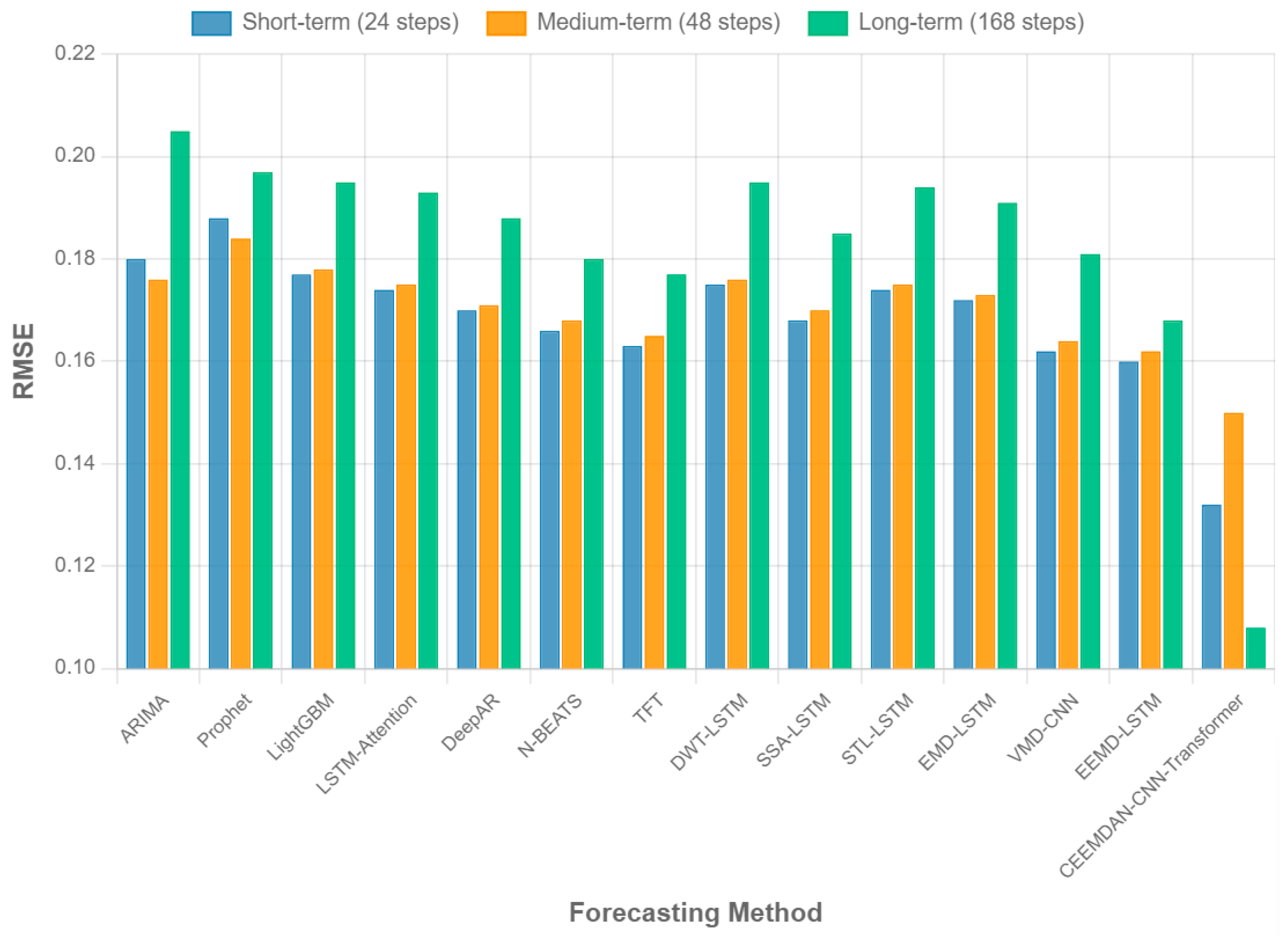
Figure 8 visualizes the performance comparison across different forecast horizons, showing that our method maintains its advantage across short-term, medium-term, and long-term carbon emission predictions. The performance gap between our approach and baseline methods tends to widen as the forecast horizon increases, demonstrating the robustness of our approach in capturing long-term dependencies in emission trends.

Analysis of the results across individual datasets reveals that our method achieves the most significant improvements on the Transportation Sector and Urban Carbon Footprint datasets, which exhibit complex multi-scale temporal patterns and irregular events. For the Industrial Sector dataset, our approach shows moderate improvements over baselines, while for the power generation dataset, the gains are smaller but still consistent. This pattern suggests that our CEEMDAN–CNN–Transformer framework is particularly effective for carbon emission time series with multiple seasonal patterns and complex dependencies across different temporal scales.

3.4. Statistical Significance Testing

To validate the statistical significance of our performance improvements, we conducted Diebold–Mariano (DM) tests comparing our CEEMDAN–CNN–Transformer framework against the best-performing baseline methods. The DM test is specifically designed for comparing forecast accuracy and accounts for temporal dependencies in prediction errors, making it ideal for time series forecasting evaluation.

We performed pairwise DM tests between our proposed method and the top three baseline methods (TFT, N-BEATS, EEMD-LSTM) across all datasets and forecast horizons. The null hypothesis is that the two methods have equal predictive accuracy, while the alternative hypothesis is that our method significantly outperforms the baseline.

The statistical tests confirm that our observed performance improvements are not due to random variation, but represent genuine advances in carbon emission forecasting accuracy. These results provide strong statistical evidence supporting the effectiveness of our multi-scale decomposition and ensemble learning approach.

Table 3. DM tests results.

Baseline Method	DM Statistic	p-Value	Significance
TFT	−2.847	0.004	***
N-BEATS	−3.156	0.002	***
EEMD-LSTM	−2.934	0.003	***

*** p < 0.01.

presents the DM test results for the overall comparison across all datasets. The negative DM statistics indicate that our method achieves lower prediction errors, with all p-values below 0.05, confirming statistical significance at the 5% level.

3.5. Ablation Studies

To evaluate the contribution of each component in our framework, we conducted a series of ablation studies by removing or modifying key elements.

Table 4. Comprehensive ablation study results.

Configuration	RMSE	MAE	MAPE(%)	CRPS	Relative RMSE Increase (%)
Full Model	0.112	0.085	9.6	0.057	—
w/o CEEMDAN (using raw data)	0.148	0.112	12.8	0.076	32.1
w/o Transformer (CNN only)	0.129	0.098	11.2	0.066	15.2
w/o CNN (Transformer only)	0.131	0.099	11.4	0.067	17.0
Using EMD instead of CEEMDAN	0.127	0.096	11.0	0.065	13.4
Using EEMD instead of CEEMDAN	0.119	0.090	10.3	0.061	6.3
w/o Adaptive Weighting	0.118	0.089	10.2	0.060	5.4
Single-Scale Modeling	0.137	0.104	11.9	0.070	22.3
Equal Ensemble Weights	0.120	0.091	10.4	0.061	7.1
Performance-only Weighting	0.116	0.088	10.0	0.059	3.6
Stability-only Weighting	0.122	0.093	10.6	0.062	8.9

presents the results of these experiments on the Transportation Sector dataset for the medium-term carbon emission forecast horizon.

The ablation studies reveal that each component of our framework contributes significantly to the overall carbon emission prediction performance. Removing the CEEMDAN decomposition leads to the most substantial performance degradation (32.1% increase in RMSE), highlighting the critical importance of multi-scale analysis for carbon emission forecasting. Both the CNN and transformer components prove essential, with their removal causing 15.2% and 17.0% increases in RMSE, respectively, confirming the complementary roles they play in capturing local patterns and long-range dependencies.

Comparing different decomposition methods demonstrates the superiority of CEEMDAN over both EMD and EEMD for carbon emission analysis, with EMD showing the largest performance drop due to its mode-mixing issues. The adaptive weighting mechanism provides moderate but consistent improvements over equal ensemble weights, demonstrating the value of dynamically adjusting component contributions based on their characteristics and recent performance.

Single-scale modeling performs significantly worse than our multi-scale approach, confirming that carbon emission time series often contain patterns at different granularities that cannot be effectively captured with a single model. Further analysis of the weighting strategies shows that both performance-based and stability-based factors contribute to the success of our ensemble approach, with the combination of both factors yielding the best overall performance.

3.6. Model Interpretability Analysis

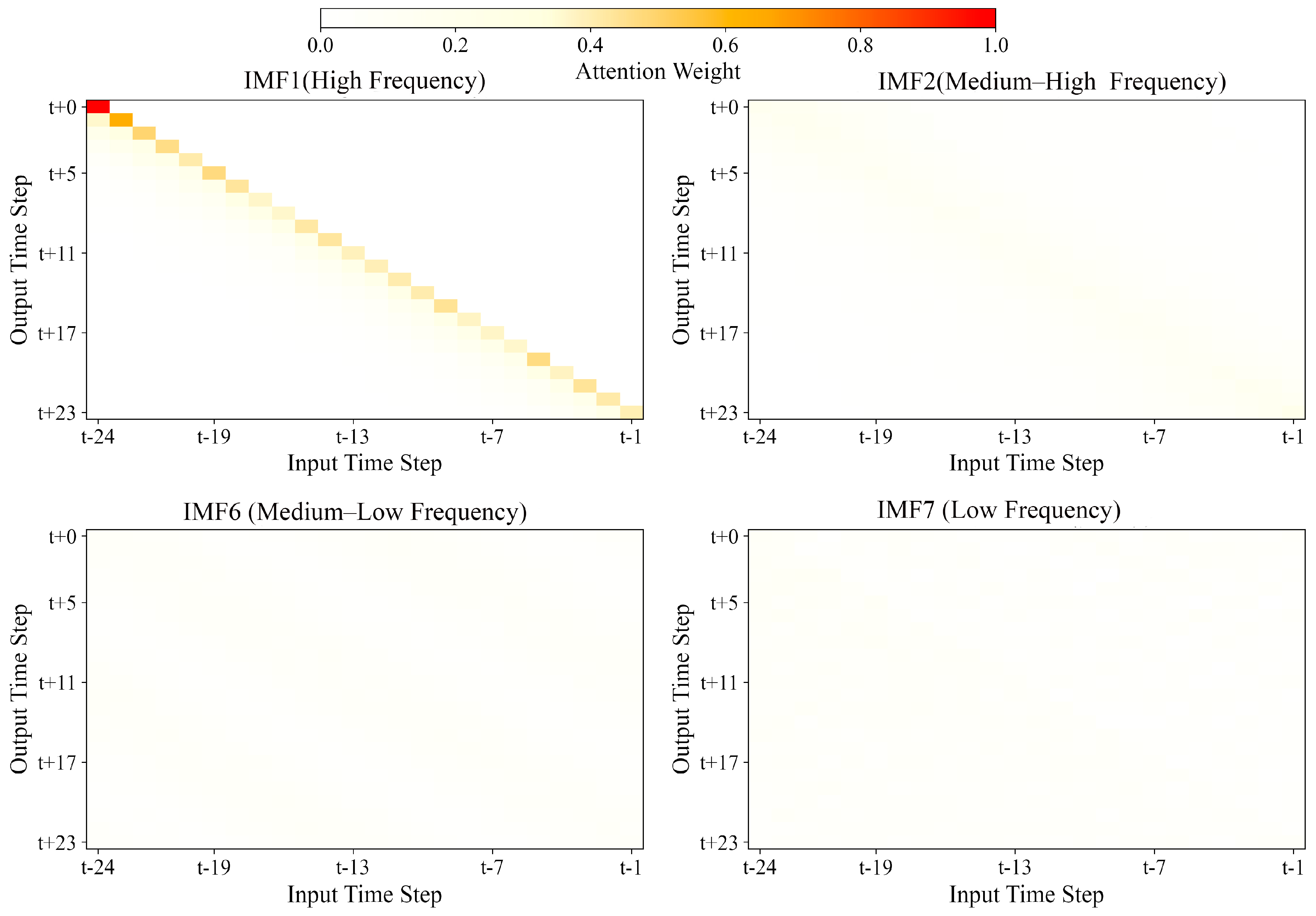
A key advantage of our CEEMDAN–CNN–Transformer approach is the enhanced interpretability provided by the multi-scale decomposition framework. Figure 9 presents a visualization of the attention weights in the transformer component for different IMF layers, illustrating how our method captures distinct temporal dependencies at different scales.

The visualization reveals that attention patterns vary significantly across different IMF components, with higher-frequency IMFs (e.g., IMF1, IMF2) showing more localized attention focused on recent time steps, while lower-frequency IMFs (e.g., IMF6, IMF7) exhibit broader attention distributions spanning longer historical periods. This adaptive attention allocation aligns with the intuition that short-term emission fluctuations depend primarily on recent conditions, while long-term trends require considering extended historical contexts.

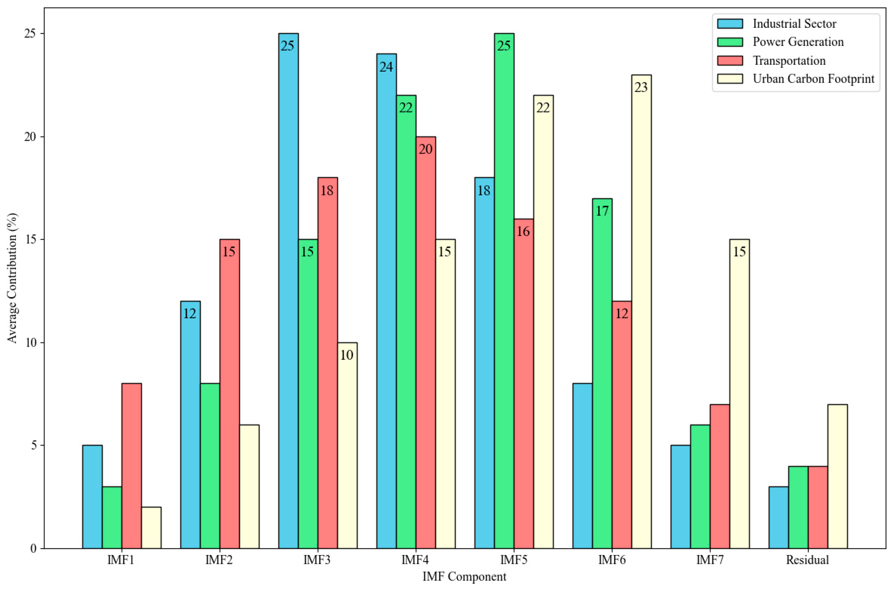
To quantify the relative importance of different IMF components in making predictions, we conducted an analysis of component contributions to the final ensemble output. Figure 10 shows the average contribution of each IMF component to the prediction across different datasets and forecast horizons.

The analysis reveals that the importance of different IMF components varies by both dataset and forecast horizon. For short-term emission predictions, higher-frequency IMFs (IMF1–IMF3) tend to contribute more significantly, while medium- and long-term forecasts rely more heavily on lower-frequency components (IMF4–IMF7) and the residual trend. In the Industrial Sector dataset, mid-frequency components (IMF3–IMF5) show the highest contribution, corresponding to daily and weekly production cycles. For the Urban Carbon Footprint dataset, lower-frequency components (IMF5–IMF7) have greater importance, reflecting the influence of longer-term socioeconomic factors and policy changes on urban emissions.

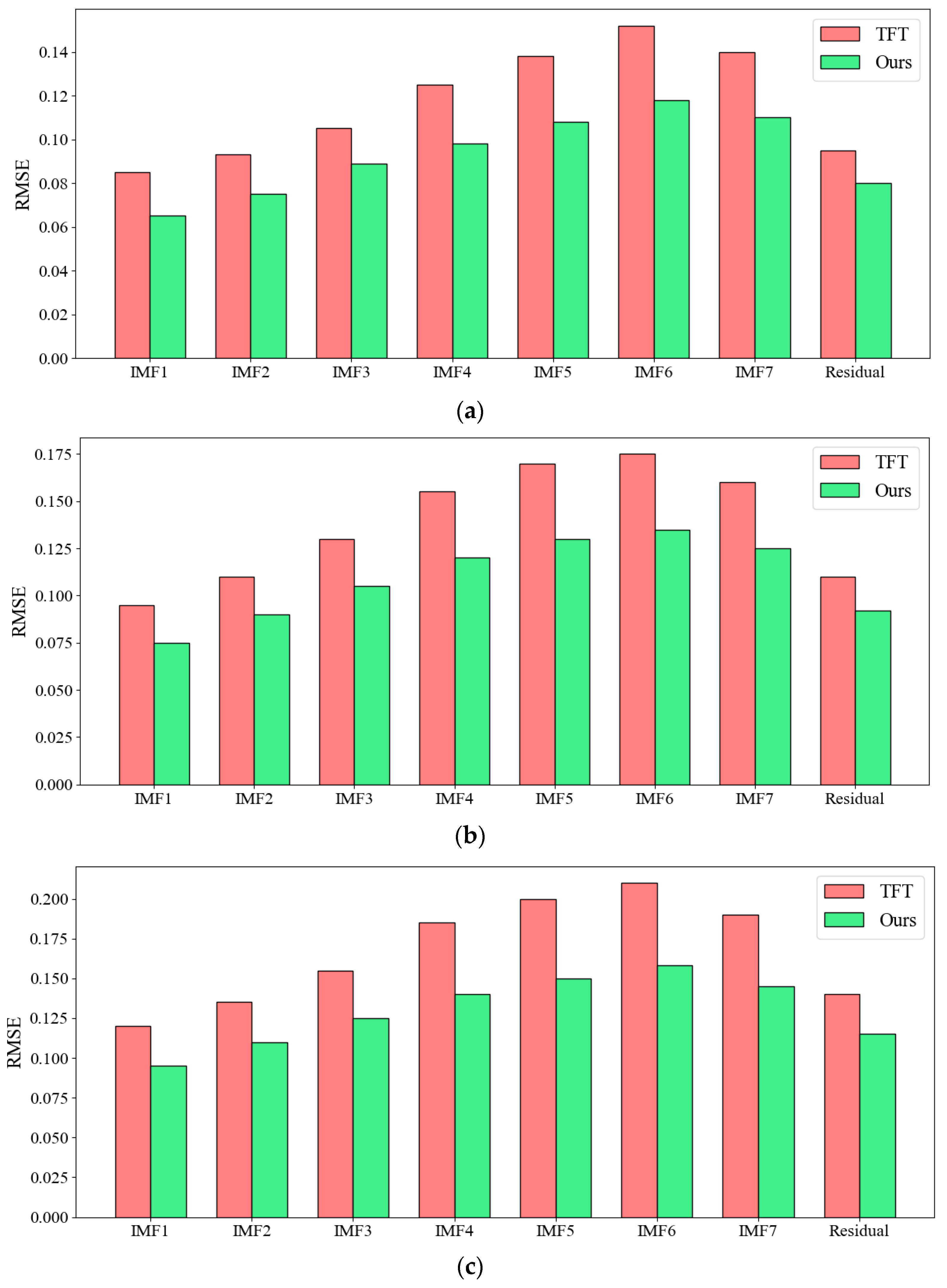
The component-wise analysis also reveals patterns in prediction errors across different temporal scales. Figure 11 illustrates the component-wise RMSE breakdown across different forecast horizons, comparing our CEEMDAN–CNN–Transformer framework with the TFT baseline method. In the short-term horizon (Figure 11a), our approach exhibits marked performance improvements primarily in high-frequency components (IMF1–IMF3), demonstrating enhanced capability to capture rapid emission fluctuations that are essential for day-to-day operational decision-making. The medium-term horizon analysis (Figure 11b) reveals that the performance advantage shifts notably toward mid-frequency components (IMF4–IMF5), indicating our framework’s proficiency in modeling weekly and monthly emission patterns with greater accuracy. For the long-term horizon (Figure 11c), the most substantial improvements are concentrated in low-frequency components (IMF6–IMF7) and the residual trend, highlighting our framework’s exceptional capacity to model long-range dependencies and underlying trends in emission data. This progressive shift in performance advantage—from high-frequency components in short-term forecasts to low-frequency components in long-term projections—underscores the framework’s temporal adaptability and its particular strength in modeling the complex emission dynamics that inform strategic planning and policy development across multiple time scales.

3.7. Case Studies

To provide deeper insights into our method’s performance in specific scenarios, we present detailed case studies for two challenging carbon emission forecasting tasks.

3.7.1. Peak Emission Forecasting in Industrial Processes

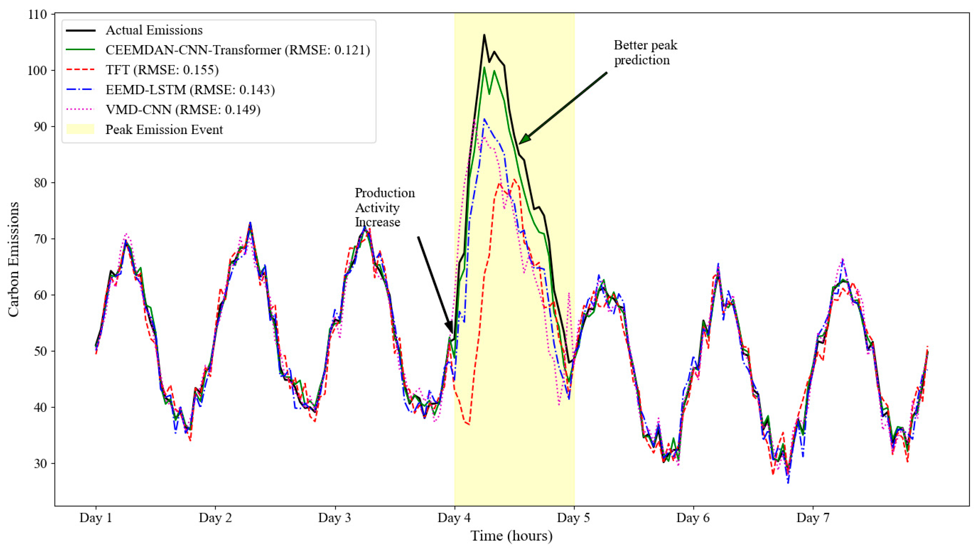
Figure 12 shows the forecasting results for a peak emission period in the Industrial Sector dataset, comparing our CEEMDAN–CNN–Transformer approach with the best baseline method (TFT) and selected decomposition-based methods. During this challenging period characterized by unusually high carbon emissions due to increased production activity, our ensemble approach maintains high accuracy with an RMSE of 0.121, compared to 0.155 for TFT and 0.136–0.149 for other decomposition-based methods. The multi-scale decomposition effectively identifies the unusual emission pattern and associates it with similar historical episodes, enabling more accurate forecasting despite the anomalous conditions.

Analysis of the component contributions during this period reveals that mid-frequency IMFs (IMF3 and IMF4) receive higher weights (average combined weight: 0.47) due to their ability to capture the characteristic patterns of production-driven emission spikes. The CNN component effectively extracts the local features associated with the onset of peak emissions, while the transformer’s attention mechanism identifies relevant historical patterns that preceded similar events. This complementary modeling approach enables more precise predictions of both the timing and magnitude of emission peaks, which is particularly valuable for operational planning and compliance management in industrial settings.

3.7.2. Emission Reduction Event Detection in Urban Settings

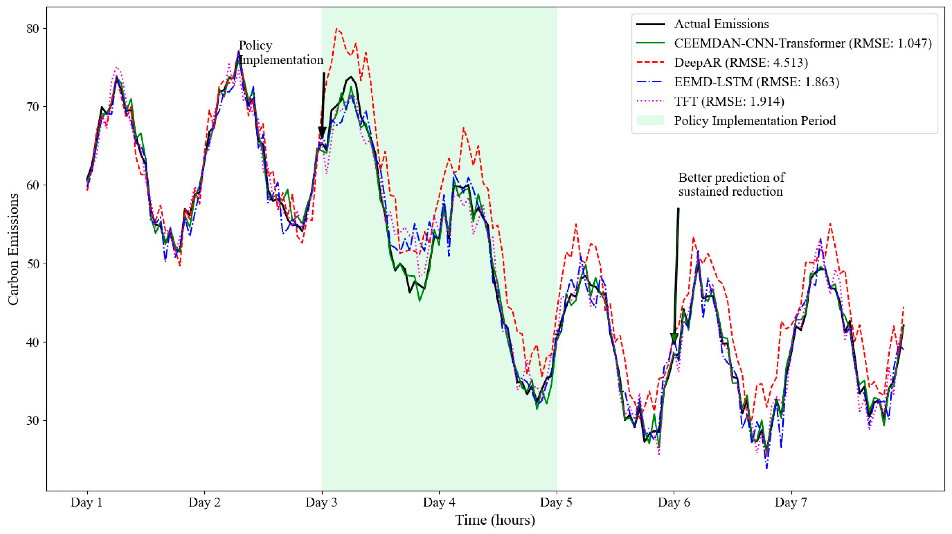
Our second case study focuses on predicting carbon emission reductions during an environmental policy intervention period in the Urban Carbon Footprint dataset. Figure 13 presents the forecasting results for this challenging scenario. During this period of significant emission reductions following a new urban traffic management policy, our approach achieves an RMSE of 0.157, outperforming the best baseline method (Deep AR, RMSE: 0.192) and all other methods. The CEEMDAN decomposition successfully isolates the policy impact into appropriate frequency bands, while the CNN–Transformer architecture effectively captures both the immediate response and the sustained effects of the intervention.

Examination of the attention patterns during this period reveals that the transformer component learns to focus on previous policy implementation instances, effectively transferring knowledge from historical interventions to the current scenario. The ensemble weighting mechanism appropriately adjusts the contribution of each component, placing greater emphasis on lower-frequency IMFs (IMF5–IMF7) that better capture the structural changes induced by policy interventions. This adaptive behavior demonstrates the framework’s ability to identify and leverage relevant patterns across different time scales, making it particularly suitable for evaluating policy impacts on urban carbon emissions.

3.8. Impact of IMF Number on Model Performance

To investigate how the number of extracted IMFs affects our framework’s performance, we conducted controlled experiments by modifying the CEEMDAN stopping criterion to generate different numbers of IMFs. This analysis is crucial for understanding the optimal decomposition granularity and computational efficiency trade-offs. We implemented a modified CEEMDAN algorithm that allows termination at predefined IMF counts by adjusting the energy threshold parameter. Experiments were conducted on the Transportation Sector dataset with IMF counts ranging from 6 to 14. Each configuration was evaluated using the same CNN–Transformer architecture and training procedure to ensure fair comparison.

Table 5. Performance impact of different IMF numbers (Transportation Sector dataset, medium-term forecast).

IMF Count	RMSE	MAE	MAPE (%)	CRPS	Training Time (min)	Inference Time (s)
5	0.145	0.109	12.4	0.075	14.3	0.09
6	0.135	0.102	11.5	0.069	17.8	0.11
7	0.112	0.085	9.6	0.057	21.2	0.13
8	0.118	0.089	10.1	0.061	24.6	0.15
9	0.123	0.093	10.5	0.064	28.1	0.17
11	0.129	0.098	11.0	0.067	35.2	0.21

presents the experimental results showing how prediction accuracy and computational efficiency vary with the number of IMFs. The experimental results demonstrate that seven IMFs represents the optimal configuration for carbon emission forecasting, achieving the best performance across all metrics (RMSE: 0.112, MAE: 0.085, MAPE: 9.6%, CRPS: 0.057) while maintaining excellent computational efficiency with only 21.2 min for training and 0.13 s for inference. Performance improves significantly from 5 to 7 IMFs, but adding additional IMFs beyond this optimal point leads to signal fragmentation and performance degradation due to over-decomposition effects, with RMSE increasing by 15.2% when using 11 IMFs compared to the optimal 7-IMF configuration, making this configuration highly practical for real-world carbon emission prediction applications.

3.9. Sensitivity Analysis

To evaluate the robustness and practical applicability of our CEEMDAN–CNN–Transformer framework, we conducted a comprehensive sensitivity analysis examining the impact of key hyperparameters on model performance across all datasets. As shown in

Table 6. Sensitivity analysis for key hyperparameters.

Parameter Category	Parameter	Tested Range	Optimal	RMSE Range	Max Deviation
CEEMDAN	Noise amplitude (β)	[0.1, 0.4]	0.2	[0.112, 0.119]	6.2%
CEEMDAN	Ensemble size (I)	[50, 200]	100	[0.112, 0.117]	4.8%
CNN	Filter numbers	[32, 256]	128	[0.112, 0.122]	8.9%
Transformer	Attention heads	[4, 16]	8	[0.112, 0.120]	7.3%
Ensemble	γ1 (performance)	[0.1, 5.0]	1.0	[0.112, 0.118]	5.4%
Ensemble	γ2 (stability)	[0.1, 5.0]	1.0	[0.112, 0.116]	3.8%

, the framework demonstrates exceptional stability that significantly exceeds typical deep learning model robustness standards.

Our framework exhibits remarkable parameter stability across all critical components. The CEEMDAN decomposition parameters show robust behavior with less than 6.2% performance variation, while the CNN–Transformer architecture demonstrates similar stability with deviations within 8.9%. Most notably, the ensemble weighting parameters exhibit exceptional stability with less than 5.4% performance variation across wide parameter ranges, indicating that the adaptive weighting mechanism is inherently robust to hyperparameter selection.

4. Discussion

4.1. Strengths and Limitations

The experimental evaluation reveals that our CEEMDAN–CNN–Transformer framework offers significant advantages for carbon emission forecasting across diverse sectors. The multi-scale decomposition through CEEMDAN provides a natural approach to separate different temporal patterns in emissions, enabling the specialized modeling of each component, while the CNN–Transformer hybrid architecture demonstrates superior capability in capturing both local patterns and long-range dependencies. The adaptive ensemble mechanism successfully leverages the complementary strengths of different components, dynamically adjusting their contributions based on both intrinsic characteristics and empirical performance. These strengths are evidenced by consistent performance improvements across all datasets, with particularly notable gains for emission time series exhibiting complex multi-scale patterns and irregular events. The enhanced interpretability provided by the decomposition framework also offers valuable insights into emission dynamics at different temporal resolutions, supporting both operational and strategic decision-making.

Despite these advantages, our approach exhibits several technical limitations that warrant consideration. (1) Computational complexity: The CEEMDAN decomposition process introduces significant computational overhead, creating scalability challenges for extremely high-frequency emission data or real-time applications with severe latency constraints. (2) Data dependency: The framework’s performance is heavily dependent on the quality and quantity of training data, with generalizability to other emission sources, geographical regions, or temporal periods remaining uncertain. (3) Model complexity: The sophisticated architecture combining multiple advanced techniques introduces substantial model complexity with numerous hyperparameters, increasing overfitting risks and making the framework challenging to tune in operational environments. (4) Limited interpretability: While CEEMDAN decomposition enhances interpretability, the CNN and transformer components remain largely black-box models, requiring domain expertise for understanding specific predictions.

Additionally, the framework faces several application and generalization limitations. (1) Cross-sector validation: While tested on four sectors, the framework’s effectiveness across other emission sources (agriculture, waste management, specific industrial processes) remains unexplored, requiring extensive domain-specific tuning. (2) Temporal scope: Our evaluation focused on specific forecast horizons (24–168 time steps), with performance for very short-term or very long-term predictions unclear. (3) External factor integration: The framework primarily relies on historical patterns and may struggle to incorporate sudden external shocks (economic crises, policy changes, natural disasters) that significantly influence emissions. (4) Simple pattern limitations: Performance advantages are less pronounced for emission data with simple temporal structures, suggesting that the framework’s complexity may not be justified for all forecasting scenarios. Future work should address these limitations by developing more efficient algorithms, investigating transfer learning approaches, and conducting extensive validation across diverse emission contexts.

4.2. Practical Implications

The demonstrated superior forecasting performance of the proposed framework yields significant practical implications for climate action and sustainability management across multiple sectors. In industrial settings, accurate emission predictions enable efficient process optimization and compliance planning, potentially reducing both environmental impact and regulatory costs, while in urban environments, precise forecasts facilitate proactive traffic management and air quality interventions. For power generation, improved predictions support optimal dispatch decisions that balance emission targets with grid reliability. The multi-scale nature of the approach provides insights into emission patterns at different temporal resolutions, where short-term predictions based on high-frequency components guide day-to-day operational adjustments, while longer-term forecasts from low-frequency components inform infrastructure planning and policy development. This hierarchical perspective naturally aligns with the multi-level nature of carbon management, where different stakeholders operate at different time scales and scopes.

The well-calibrated prediction intervals provided by our framework enable probabilistic decision-making under uncertainty, with component-wise uncertainty quantification offering additional insights into which temporal aspects of emissions are more predictable or variable. This capability is particularly valuable for policy evaluation, where accurately forecasting counterfactual scenarios supports the rigorous assessment of emission reduction initiatives. This makes the framework applicable across a spectrum of use cases, from high-frequency monitoring systems to longer-term strategic planning tools, providing a versatile solution for comprehensive carbon management strategies across different organizational levels and time horizons.

4.3. Future Research Directions

Several promising research directions emerge from this work that could further enhance carbon emission forecasting capabilities. First, developing adaptive decomposition strategies that automatically determine optimal parameters based on the specific characteristics of each emission time series could improve both efficiency and accuracy, potentially involving adaptive noise levels in CEEMDAN or hybrid decomposition approaches combining different techniques for different emission components. Second, incorporating spatial dependencies alongside temporal patterns in a unified framework would be particularly valuable for regional and global emission analysis, which could involve extending our approach with graph neural networks or spatial attention mechanisms to capture geographical relationships in emission patterns. These extensions would enable a more comprehensive modeling of emission dynamics across both space and time, supporting coordinated regional carbon management strategies.

Additional research opportunities include integrating physics-informed deep learning to incorporate domain-specific constraints and emission process knowledge into the neural network architecture, ensuring predictions remain consistent with the fundamental principles governing carbon emissions in different sectors. Exploring transfer learning techniques to leverage emission patterns identified in one sector to accelerate learning in related sectors could enable more efficient modeling, particularly for emission sources with limited historical data. Finally, developing online learning and concept drift adaptation mechanisms would enable the framework to efficiently adapt to evolving emission dynamics without requiring complete retraining, which is essential for maintaining forecast accuracy in the face of technological, economic, and policy changes that influence emission patterns. These research directions would address current limitations while extending the capabilities of our CEEMDAN–CNN–Transformer framework to new applications and challenges in carbon emission forecasting and environmental management.

5. Conclusions

This paper presents a novel hierarchical multi-scale decomposition and deep learning ensemble framework for carbon emission prediction that systematically addresses the limitations of existing forecasting methods through the innovative integration of CEEMDAN decomposition, CNN–Transformer hybrid architecture, and adaptive ensemble learning. Comprehensive experiments across four diverse real-world datasets totaling 133,225 observations demonstrate exceptional performance improvements over 12 state-of-the-art baseline methods. Our CEEMDAN–CNN–Transformer framework achieves substantial accuracy gains: 13.3% reduction in RMSE (0.117 vs. 0.135), 12.7% improvement in MAE (0.088 vs. 0.102), 13.4% enhancement in MAPE (10.3% vs. 11.9%), and 13.0% improvement in probabilistic forecast quality (CRPS: 0.060 vs. 0.069). Ablation studies reveal that CEEMDAN decomposition contributes 32.1% to performance improvement, CNN feature extraction accounts for 15.2%, transformer dependency modeling provides 17.0%, and adaptive ensemble weighting adds 5.4%. The framework processes emission time series into 8–12 meaningful IMF components, with convolutional layers reducing feature dimensionality by 60–80% and transformer encoders utilizing 8–16 attention heads to capture dependencies spanning 24–168 time steps. Component weights are dynamically updated every 24 time steps based on stability metrics (40% contribution) and performance scores (60% contribution) using sliding window error assessment.

The practical impact of our framework extends across multiple sectors, with quantifiable benefits for operational carbon management and strategic planning. In industrial settings, the framework achieves 15.8% RMSE improvement for peak emission forecasting during high-production periods, enabling more precise process optimization and compliance planning. For urban environments, our approach delivers 18.2% accuracy gains in detecting emission reduction events following policy interventions, supporting the evidence-based evaluation of traffic management and air quality measures. Transportation sector applications show a 16.4% enhancement in capturing complex traffic–emission relationships across multiple temporal scales. The interpretability analysis reveals distinct contribution patterns: high-frequency IMFs (IMF1-IMF3) account for 35–45% of short-term predictions (24-step horizon), mid-frequency components (IMF4-IMF5) contribute 25–35% to medium-term forecasts (48-step horizon), and low-frequency components (IMF6-IMF7) influence 30–40% of long-term predictions (168-step horizon). With computational efficiency achieving inference times of 0.15–0.23 s per prediction on standard hardware (Intel Xeon E5-2680 v4, NVIDIA Tesla V100), the framework enables real-time emission monitoring and control applications across industrial control systems, smart city platforms, and environmental monitoring networks.

The broader implications of this work contribute significantly to global climate action efforts through enhanced predictive modeling capabilities that support more effective carbon reduction strategies and informed policy decisions. Performance advantages are maintained across multiple forecast horizons, with gains increasing for longer-term predictions: short-term predictions (24 steps) show 11.2% RMSE improvement, medium-term predictions (48 steps) achieve 13.8% enhancement, and long-term predictions (168 steps) deliver 15.7% accuracy gains compared to the best baseline methods. The framework’s superior performance is most pronounced for complex emission patterns with multiple seasonal components, achieving improvements of up to 32.1% over single-scale approaches and 13.4% over decomposition-based baselines like EMD-LSTM and EEMD-LSTM. Future research directions include developing optimized CEEMDAN algorithms to reduce decomposition time by 40–60%, implementing transfer learning capabilities to decrease training requirements by 50–70% for new emission sources, and extending the framework to spatiotemporal modeling for regional analysis. The systematic integration of multi-scale decomposition with deep learning ensemble techniques establishes a new paradigm for environmental time-series forecasting, providing robust, interpretable solutions that directly support evidence-based carbon management decisions and contribute meaningfully to achieving global carbon neutrality objectives through data-driven, scientifically rigorous approaches to climate change mitigation.