Curvature-Based Change Detection in Road Segmentation: Ascending Hierarchical Clustering vs. K-Means

Abstract

This work addresses the challenge of low-cost road quality monitoring in the context of developing countries. Specifically, we focus on utilizing accelerometer data collected from smartphones as drivers traverse roads in their vehicles. Given the high frequency of data collection by accelerometers, the resulting large datasets pose a computational challenge for anomaly detection using supervised classification algorithms. To mitigate scalability issues, it is beneficial to first group the data into homogeneous continuous sections. This approach aligns with the broader problem of change detection in a finite sequence of data indexed by a totally ordered set, which could represent either a time series or a spatial trajectory. Curvature features are extracted and segmented through adapted Ascending Hierarchical Clustering (AHC) and K-means algorithms suited to sequential road data. Our goal is to segment roads into homogeneous sub-sections that can subsequently be labeled based on the level or type of irregularity. Using an analysis of variance (ANOVA) statistical test, we demonstrate that curvature features are effective for classification, with a Fisher value of $14.28$ and a p-value of $9.77\times {10}^{-7}$. We use two change detection algorithms: (1) Ascending Hierarchical Clustering (AHC) and (2) K-means. Based on the dataset and the number of classes, AHC and K-means achieve the following performance metrics, respectively: specificity of $85.52\%$ and $87.48\%$, true negative rate of $93.6\%$ and $93.73\%$, accuracy of $84.18\%$ and $82.59\%$, $\kappa$-coefficient of $84.18\%$ and $82.56\%$, and Rand index of $86.33\%$ and $82.84\%$. The average computational time for K-means is $333.1$ s, compared to $0.312$ s for AHC, resulting in a ratio of 1070. Overall, AHC is significantly faster and achieves a better balance of performance compared to K-means.

1. Introduction

Standard French Norm “NF EN 13306: 01 2018” (European standard for maintenance terminology) defines maintenance as all technical, administrative and management actions during the life cycle of a system, intended to maintain or restore it to a state in which it can perform its required function. An important aspect of maintenance is the diagnosis of failures. The failure of a system can lead to more or less serious consequences. This is particularly true for roads, which are of vital importance for development. In economic terms, poor road quality entails direct costs such as repairs to damaged vehicles, as well as indirect costs such as reduced productivity due to displacement difficulties [1]. In addition to the purely economic aspect, road failures can cause social trauma. Over the past decade, the rate of road traffic deaths has risen dramatically in Africa, resulting in the loss of nearly 250,000 in human lives by 2021 (https://www.afro.who.int/fr/news/les-deces-dus-aux-accidents-de-la-circulation-augmentent-dans-la-region-africaine-mais) (13 December 2024). According to the World Health Organization (WHO, Geneva, Switzerland), there will be around $1.19$ million traffic-related deaths worldwide in 2023 (https://www.who.int/fr/news/item/13-12-2023-despite-notable-progress-road-safety-remains-urgent-global-issue) (13 December 2024). Therefore, it is very important to develop mechanisms for monitoring road quality. This would make it possible to identify failures and assess the corrective actions required.

Many works in the literature deal with the detection of road anomalies. This detection is generally carried out by analyzing data collected by various sensors. In general, it involves the analysis of images taken by various means [2,3,4], the vibratory analysis, or the kinematic analysis of the road course [5,6,7,8]. The images obtained are then processed by algorithms to detect irregularities. Image analysis benefits from technological advances in image processing and computer vision. However, the quality of detection can be altered by environmental factors such as luminosity or weather conditions. For vibration and kinematic analysis, inertial sensors such as Global Positioning Systems (GPS), accelerometers and gyroscopes built into smart phones or vehicles are used. This last group of sensors seems more accessible in the context of developing countries, where a large proportion of vehicles in circulation are second-hand and in a relatively advanced state of amortization [9]. For example, $92\%$ of Cameroon’s vehicle fleet is made up of vehicles acquired second-hand and are more than 15 years old (https://www.investiraucameroun.com/transport/1706-6454-92-du-parc-automobile-camerounais-est-constitue-de-vehicules-acquis-en-seconde-main) (13 December 2024).

Regardless of the type of road status data collected as time series, classifying this data is essential. This process involves two phases. The first phase consists of segmenting the time series into homogeneous sequences. Groups of homogeneous points are then labeled with predefined road types. In the second phase, automatic classification models are often trained in a supervised manner [5,6,7]. Classification is based on the characteristics extracted and the segmentation performed in the first phase [10,11]. The final performance of the models is highly sensitive to this step. The segmentation problem is equivalent to change detection, which is frequently addressed using unsupervised learning algorithms [12,13,14,15].

Unsupervised learning algorithms seek to identify underlying structures in data. In particular, clustering algorithms aim to group sets of data into subsets or ’clusters’, based on similarity or distance between data points [16]. Some works exploit clustering to evaluate the change between several time series [17,18]. However, in the context of this work, we aim to detect change in the same time series. Tran is part of this approach in [15] by proposing a real-time segmentation algorithm using a dynamic K-means algorithm based on Euclidean distance. In the same vein, the authors of the reference [19] propose the SWAB algorithm, which creates classes using a spline-based interpolation error minimization approach. These important general works do not dwell particularly on the extraction of classification features. However, it is common practice in data science to take into account the particularities of the application domain. For example, to avoid obstacles or adapt to road irregularities, drivers are often forced to adjust their trajectory, which then becomes less regular. Indeed, since the quality of the road is linked to its geometry, it seems natural to extract geometric characteristics from driving trajectories. On the other hand, since the segmentation of a time series can be reduced to a binary label, existing classification algorithms could be adapted or even improved.

This work tackles the problem of detecting changes in road conditions using road access data. The aim is to segment a given road into homogeneous sub-sections for labeling according to the level or type of irregularity. The aim is to develop and evaluate algorithms for change detection and to compare their performance on sets of real data. The research hypotheses are that (1) curvatures are relevant characteristics for classifying road irregularities, and (2) the bottom-up hierarchical classification algorithm is faster and more efficient than the K-means algorithm for this task. Our contributions are as follows:

• We pre-process the data before labeling by reducing its dimensionality through segmentation, which is a specific form of clustering.
• We propose features that better characterize changes in road structure.
• We adapt abstract algorithmic approaches -specifically, AHC and k-means- to road segmentation.
• We demonstrate that the segmentation problem in time series is analogous to binary classification or $\left\{0,1\right\}$-labeling, enabling the use of a confusion matrix for evaluating the performance of the proposed algorithms.
• We introduce a novel change detection metric called the rate of agreement with the change.

The rest of the article is organized as follows. Section 2 presents an overview of the state of the art and Section 3 describes the methodology used. Section 4 presents results and discussions, while Section 5 concludes the work and offers future perspectives.

2. Related Work

2.1. Road Condition Detection and Classification

The detection of anomalies on the road surface using mobile sensing has been extensively explored through supervised approaches. Basavaraju et al. (2019) proposed a supervised model to classify road surface anomalies such as potholes and cracks using vibration data and images. Their system employed support vector machines and neural networks for multi-class classification, but required fully labeled training data [20]. Nguyen et al. (2019) developed a crowdsourcing-based solution that combines vibration and GPS data from smartphones. Their system uses adaptive thresholding and spatial clustering to detect and map surface defects. Despite its practical implementation, the approach lacks a segmentation mechanism and depends heavily on parameter tuning [21]. Wu et al. (2020) introduced a machine learning pipeline for pothole detection using smartphone accelerometers. It features a preprocessing stage followed by supervised classification. While effective, the model is focused on binary detection and is reliant on well-annotated datasets [22]. Rajput et al. (2022) designed an unsupervised framework for monitoring road conditions using vibration data from public transport vehicles. By exploiting the regular motion of buses, they detect irregular road segments without the need for training labels, offering a scalable alternative for smart city deployment [23]. Bustamante et al. (2022) proposed a shallow neural network to classify road types based on smartphone accelerometer readings. Although their method achieved promising classification accuracy, it does not incorporate any temporal segmentation process [24]. Kim et al. (2024) presented a deep learning architecture combining CNN and LSTM to detect road anomalies from spatiotemporal sequences. Their work emphasizes learning temporal dependencies in road condition monitoring, but is computationally intensive and less suitable for low-resource environments [25]. Recent advances in land cover and land use mapping from satellite time-series, demonstrate the potential of remote sensing for detecting large-scale changes in infrastructure, including roads [26]. However, such products typically offer limited spatial and temporal resolution, which constrains their ability to capture fine-grained features like local curvature variations, small-scale surface anomalies, or gradual structural degradation. In contrast, our approach based on vehicle-mounted inertial and GPS sensors provides a more detailed, ground-level perspective. These two approaches are therefore complementary: satellite data is useful for macro-scale monitoring, while sensor-based methods are better suited for localized, high-resolution road condition assessment.

2.2. Trajectory Segmentation

Several studies have investigated trajectory segmentation. Van Kuppevelt et al. (2019) proposed an unsupervised method to segment daily-life accelerometer signals using a Hidden Semi-Markov Model. Their approach segments sensor data into behavioral states without requiring labels, showcasing the feasibility of structure discovery in time series [27]. Etemad et al. (2019) introduced a trajectory segmentation algorithm based on interpolation and clustering. Their method automatically detects homogeneous movement phases by minimizing interpolation errors in an unsupervised way, without assuming prior knowledge of trajectory labels [28]. Tapia et al. (2024) designed an unsupervised gesture recognition framework that uses curvature and its derivative to segment continuous movement trajectories. Although applied in robotics and gesture domains, their curvature-based approach shares conceptual similarities with our method for road segmentation [29]. In order to better understand our contribution, it seems appropriate to focus on fundamental segmentation methods based on data in the form of time series, sometimes acquired in real time.

2.2.1. Sliding Window and Bottom up Method

The SWAB method proposed in [19] is a combination of bottom-up clustering and the sliding window clustering that facilitates real-time segmentation of a time series flow. The authors in [19] seek the best interpolation of a time series using linear splines. The pieces of linearity also define a partition of the series into classes. Given a class C, the corresponding spline is obtained by linear regression ($line\left(C\right)$) and the maximum absolute estimation error must not exceed a given threshold ($max\_error\left(line\left(C\right),C\right)\le \epsilon$). Given an integer $N\in \mathbb{N}$ (excluding 0), the size of a class is bounded between $N/2$ and $2N$. It is also limited by the maximum absolute estimation error.

The Algorithms 1 and 2 are adapted versions of the bottom-up algorithm and SWAB algorithm discussed in [19]. The current descriptions of these algorithms remain fundamentally identical to the original versions. However, they are now closer to practical implementation. Letting n be the length of time series T, the respective complexities of Algorithms 1  and 2 are $O\left(n^4\right)$ and $O\left(n\times N^4\right)$. Indeed, the complexity of regression function named “line” is $O\left(N^2\right)$, there are nested loops and Algorithm 2 calls Algorithm 1.

Algorithm 1 BUA (T: Time Series, $\epsilon$: error threshold)

$Cl\leftarrow$ {} $i\leftarrow 1$ while $\left(i\le length\left(T\right)-3\right)$  do    $Cl\leftarrow Cl\cup \left\{\left\{T\left[i\right],T\left[i+1\right]\right\}\right\}$    $i\leftarrow i+1$ end while $Cl\leftarrow Cl\cup \left\{\left\{T\left[i\right],\dots ,T\left[length\left(T\right)\right]\right\}\right\}$ $idx\leftarrow 1$ $e_{min}\leftarrow max\_error\left(line\left(Cl\left[idx\right]\cup Cl\left[idx+1\right]\right),Cl\left[idx\right]\cup Cl\left[idx+1\right]\right)$ for $i\leftarrow 2$ to $length\left(Cl\right)-1$ do    if $\left(max\_error\left(line\left(Cl\left[i\right]\cup Cl\left[i+1\right]\right),Cl\left[i\right]\cup Cl\left[i+1\right]\right)<e_{min}\right)$ then      $idx\leftarrow i$      $e_{min}\leftarrow max\_error\left(line\left(Cl\left[idx\right]\cup Cl\left[idx+1\right]\right),Cl\left[idx\right]\cup Cl\left[idx+1\right]\right)$    end if end for while $\left(e_{min}<\epsilon \right)$ and $\left(length\left(Cl\right)\ge 2\right)$ do    $Cl\left[idx\right]\leftarrow Cl\left[idx\right]\cup Cl\left[idx+1\right]$    $Cl\leftarrow Cl\setminus Cl\left[idx+1\right]$    $idx\leftarrow 1$    $e_{min}\leftarrow max\_error\left(line\left(Cl\left[idx\right]\cup Cl\left[idx+1\right]\right),Cl\left[idx\right]\cup Cl\left[idx+1\right]\right)$    for $i\leftarrow 2$ to $length\left(Cl\right)-1$ do      if $\left(max\_error\left(line\left(Cl\left[i\right]\cup Cl\left[i+1\right]\right),Cl\left[i\right]\cup Cl\left[i+1\right]\right)<e_{min}\right)$ then         $id\leftarrow i$         $e_{min}\leftarrow max\_error\left(line\left(Cl\left[idx\right]\cup Cl\left[idx+1\right]\right),Cl\left[idx\right]\cup Cl\left[idx+1\right]\right)$      end if    end for end while Return $Cl$

Algorithm 2 SWAB (T: Time Series, N: Window’s length, $\epsilon$: error threshold)

$Cl1\leftarrow$ {} /* Temporary cluster*/ $Cl2\leftarrow$ {} /* Final cluster*/ $anchor\leftarrow 1$ $W\leftarrow$ {} /* The window*/ while ($anchor\le length\left(T\right)$) do    $idx\leftarrow min\left(anchor+max\left(0,N/2-length\left(W\right)-1\right),length\left(T\right)\right)$    $W\leftarrow W\cup \left\{T\left[anchor\right],\dots ,T\left[idx\right]\right\}$    $idx\leftarrow idx+1$    $condition\leftarrow$ ($idx\le length\left(T\right)$) and ($length\left(W\right)<2N$)    $condition\leftarrow condition$ and ($max\_error\left(line\left(W\cup \left\{T\left[idx\right]\right\}\right),W\cup \left\{T\left[idx\right]\right\}\right)\le \epsilon$)    while $condition$ do      $W\leftarrow W\cup \left\{T\left[idx\right]\right\}$      $idx\leftarrow idx+1$      $condition\leftarrow$ ($idx\le length\left(T\right)$) and ($length\left(W\right)<2N$)      $condition\leftarrow condition$ and ($max\_error\left(line\left(W\cup \left\{T\left[idx\right]\right\}\right),W\cup \left\{T\left[idx\right]\right\}\right)\le \epsilon$)    end while    $Cl1\leftarrow BUA\left(W,\epsilon \right)$    $Cl2\leftarrow Cl2\cup \left\{Cl1\left[1\right]\right\}$    $W\leftarrow W\setminus Cl1\left[1\right]$    $anchor\leftarrow anchor+length\left(Cl1\right[1\left]\right)$ end while Return $Cl2$

2.2.2. Overlapping Windows Method

The overlapping windows method consists in selecting two blocks of data of the same size N having $N-1$ points in common. The time series is considered as a set in a $d+1$ dimensional space-time. The first block is partitioned into K disjoint groups using K-means algorithm. For each class the size, the mean (centroid) and the standard deviation (radius) vectors are computed and saved as an abstract class. The mean and the standard deviation vectors are calculated dimension by dimension. A point in the second block belongs to an abstract class if according to each dimension, the Euclidean distance (usual distance in the real line) between it and the centroid is less or equal to the corresponding standard deviation component. Thus, to be member of an abstract class is the success of $d+1$ tests. A point that does not belong to any abstract class is considered as a change point. Algorithm 3 is an adaptation of Algorithm 1 presented in [15]. Although K-means is a stochastic methods we can estimate the complexity of Algorithm 3 as $O\left(n\times K^{N-1}\right)$. This comes from the fact that the number of possible partitions in K subsets of a set of with N element is $\left(K-1\right)!{\sum }_{\ell =1}^K{\left(-1\right)}^{K-\ell }{\ell }^{N-1}/\ell !$.

Algorithm 3 OWA (T: Time Series, N: Length of the window, K: Number de Clusters)

$Cl\leftarrow$ {} /* The final cluster*/ $L\leftarrow length\left(T\right)$ $pos1\leftarrow 1$ /* The current position of a first cursor in T */ $w1\leftarrow \left\{T\left[i\right];pos1\le i\le min\left(pos1+N-1,L\right)\right\}$ $C\leftarrow \mathrm{K}-\mathrm{means}(w1,min\left(K,min\left(pos1+N-1,L\right)-pos1+1\right))$ /* C is a cluster from $w_1$ in K classes */ $pos2\leftarrow min\left(pos1+1,L\right)$ /* The current position of a second cursor in T */ $w2\leftarrow \left\{T\left[i\right];pos2\le i\le min(pos2+N-1,L)\right\}$ while ($pos2<L$) do    if ($change\left(C,pos2\right)$) or ($pos2=pos1+N$) then      $Cl\leftarrow Cl\cup \left\{\left\{T\left[pos1\right],\dots ,T\left[pos2-1\right]\right\}\right\}$      $pos1\leftarrow pos2$      $pos2\leftarrow min\left(pos1+1,L\right)$      $w1\leftarrow \left\{T\left[i\right];pos1\le i\le min\left(pos1+N-1,L\right)\right\}$      $C\leftarrow \mathrm{K}-\mathrm{means}(w1,min\left(K,min\left(pos1+N-1,L\right)-pos1+1\right))$    else      $pos2\leftarrow min\left(pos2+1,L\right)$    end if    $w2\leftarrow \left\{T\left[i\right];pos2\le i\le min(pos2+N-1,L)\right\}$ end while Return $Cl$

Table 1. Extended comparison of related works on unsupervised and supervised road and trajectory analysis.

Year	Ref.	App. Type	Road Mon.	Curv.	Segm.	Data Type	Feature Extraction	Application Domain	Evaluation Metrics
2019	[27]	Uns.	No	No	Yes	Accele- rometer	Time-windowed signal embeddings	Human Activity Monitoring	qualitative analysis
2019	[28]	Uns.	No	No	Yes	Generic trajectory data	Interpolation-based descriptors	Trajectory Mining	Interpolation error, temporal accuracy
2019	[20]	Sup.	Yes	No	No	Accele- rometer/image	Raw image + vibration amplitudes	Road Surface Classification	Accuracy, Precision, Recall, F1-score
2019	[21]	Sup.	Yes	No	No	Accele- rometer & GPS	Spatial features, GPS thresholds	Road Condition Detection	Detection rate, False positive rate
2020	[22]	Sup.	Yes	No	No	Accele- rometer	FFT, Mean, std, skewness, kurtosis, RMS	Road Condition Monitoring	Accuracy, Precision, Recall, AUC
2022	[23]	Uns.	Yes	No	Yes	Accele- rometer	Extreme Value, variance	Road Monitoring (Bus)	Silhouette score, qualitative map
2022	[24]	Sup.	Yes	No	No	Accele- rometer	Mean, min, max, std, energy computed	Road Condition Monitoring	Accuracy, Confusion Matrix
2024	[25]	Sup.	Yes	No	No	Spatio- temporal sequences	Learned features (CNN, LSTM, RF)	Road Condition Mapping	Precision, Recall, F1-score, MAE, RMSE
2024	[29]	Uns.	No	Yes	Yes	Trajectory gestures	Curvature + curvature derivative	Gesture segmentation via curvature	Segmentation accuracy, Levenshtein distance
2025	Our work	Uns.	Yes	Yes	Yes	Accelerometer	Curvilinear abscissas, curvatures	Road Segmentation and Change Detection	Accuracy, F1-score, Rand Index, ARI, $\kappa$,
									Change Agreement Rate

Legend: Ref. = Reference; App. Type = Approach Type; Uns. = Unsupervised; Sup. = Supervised; Road Mon. = Road Monitoring; Curv. = Uses Curvature; Segm. = Performs Segmentation.

summarizes the most relevant studies related to the detection of road condition and the segmentation of the trajectory. Supervised methods (e.g., [22,25]) offer high classification accuracy but rely on labeled data and do not perform explicit segmentation. Unsupervised works (e.g., [27,29]) focus on structural analysis but rarely target road data or leverage geometric descriptors. Our method bridges these gaps by combining curvature-based features, a custom dissimilarity metric, and adaptations of AHC and K-means for time-series segmentation. It stands out for being fully unsupervised, label-free, and tailored to road structure analysis-making it more suitable for deployment in resource-constrained environments.

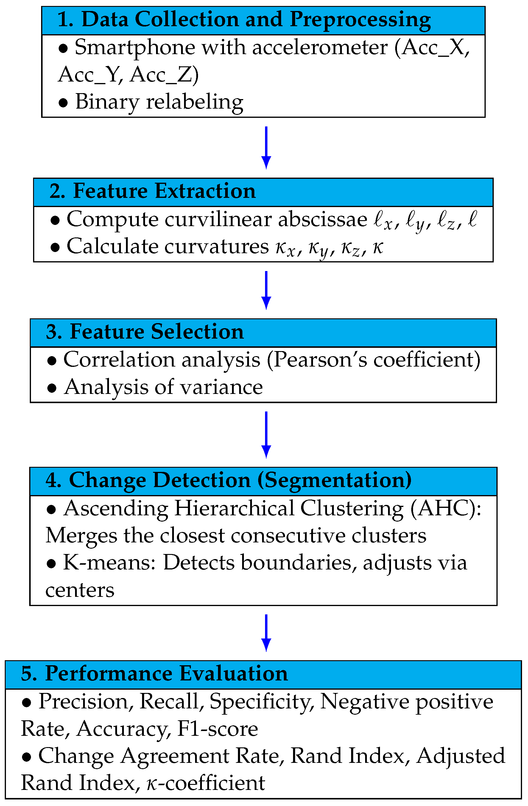
3. Methodology of the Work

The detection of road irregularities can be divided into two main stages: (1) the detection of changes and (2) the characterization or labeling of these changes. In this work, we focus on the first stage, which involves segmenting the road into a series of relatively homogeneous sections or classes. Since the objective is not directly labeling, we employ unsupervised approaches to classification.

The proposed methodology consists of five steps: (1) Collection and preprocessing of accelerometer data, where smartphone sensors record vibrations along road segments. (2) Feature extraction is performed using numerical integration and differentiation techniques to calculate curvilinear abscissas and curvatures. (3) Feature selection, where correlation and variance analyses are used to retain the most discriminative attributes. (4) Change detection is carried out using adapted versions of Ascending Hierarchical Clustering (AHC) and K-means, tailored to the sequential nature of the data. (5) Performance evaluation of the resulting segmentation using both classical metrics (e.g., Precision, Recall, F1-score) and additional measures such as the Adjusted Rand Index and the Change Agreement Rate. The overall methodological framework adopted in this study is summarized in the workflow presented in Figure 1. The proposed methodology is generalizable and remains applicable regardless of sensor frequency, driving behavior, or environmental conditions.

3.1. Data Collection and Pre-Processing

Detecting points of change on a road involves monitoring information that is characteristic of the route. These characteristics are varied in nature (sounds, images, etc.) and may require specialized and costly hardware. As our objective is to propose effective solutions for contexts with limited resources, we have opted for data that is relatively easy to access via an accelerometer integrated with current equipment such as a smart phone. We use the trajectories of the vehicles to assess any changes in the nature of the road.

3.1.1. Description of the Dataset

We use a dataset collected on various road sections using a smartphone equipped with a accelerometer for acceleration measurements. These sensors provided samples at a frequency of 10 Hz. The data, previously used in [11] for supervised classification, are available in CSV format via the following URL: https://github.com/simonwu53/RoadSurfaceRecognition/blob/master/data/sensor_data_v2.zip (13 November 2024). The accelerometer data used in this study were already preprocessed by the dataset authors [11].

• Timestamps: sampling instants in milliseconds.
• Raw data: raw measurements of the components of the acceleration vector for the X, Y and Z axes.
• Adjusted data: Adjusted access data from the telephone’s co-ordination system for a universal co-ordination system.
• Route labels: character string that can take the values ’smooth’, ’bumpy’ or ’rough’.

The main characteristics of the dataset used in this study, including data types, sources, resolution, acquisition devices, and labeling information, are summarized in

Table 2. Summary of dataset characteristics used in the study.

Attribute	Description
Data types	Accelerometer signals (accX, accY, accZ)
Data source	github.com/simonwu53/.../sensor_data_v2.zip (13 November 2024)
Data resolution	10 Hz sampling frequency
Data acquisition date	2020
Device used	Smartphone with built-in accelerometer

.

The data is enriched by secondary information calculated on the basis of the first data collected: curvilinear abscissa (ℓs) and curvatures (${\kappa }_i$s). Since only the changes are of interest, the data are relabeled with binary values. In this approach, changes are represented by transitions from 0 to 1 or from 1 to 0, as illustrated in

Table 3. Labeling of data.

N°	Textual Label		Binary Label
1	Smooth	→	0
2	Bumpy	→	1
3	Bumpy	→	1
4	Bumpy	→	1
5	Rough	→	0

. The sequence of labels $\left(0,1,1,1,0\right)$ corresponds to the following three classes: $Clas{s}_1=\left\{1\right\}$, $Clas{s}_2=\left\{2,3,4\right\}$, and $Clas{s}_3=\left\{5\right\}$. This labeling aligns with the logical framework for change detection described in [15]. The curvilinear abscissas in each direction of the orthonormal basis of Cartesian space, and the associated curvatures, are also added to the data, as shown in

Table 4. Dataset structure.

Measurements Available in the Dataset					Calculated by Ourselves
Timestamp	$ac{c}_x$	$ac{c}_y$	$ac{c}_z$	Textual label	Binary label	${\ell }_x$	${\ell }_y$	${\ell }_z$	ℓ	${\kappa }_x$	${\kappa }_y$	${\kappa }_z$	$\kappa$

.

3.1.2. Extraction of Features

The features used in this work are the curvilinear abscissa (ℓ) and curvatures (${\kappa }_i$), computed using acceleration data from accelerometers. The primary advantage of using curvatures is that they generally capture the intrinsic characteristics of a trajectory, independent of velocity. As a result, the information about the road condition conveyed by curvatures is likely to be more robust. This approach helps mitigate the issue of sampling frequency highlighted in [6]. Large curvature values indicate significant or frequent irregularities, while a constant curvature provides insights into the shape of the road, which can be useful for the labeling process. Curvature can be sensitive to noise and sensor drift. However, the data set used in this study was pre-processed and denoised. For further theoretical details of curvatures, we refer to [30].

Considering the trajectories $\left(t,x\left(t\right)\right)$, $\left(t,y\left(t\right)\right)$, $\left(t,z\left(t\right)\right)$ and $\left(t,x\left(t\right),y\left(t\right),z\left(t\right)\right)$ the curvilinear abscissas are respectively given through the following formulas:

$${\ell }_x\left(t\right)={\int }_{t_0}^t\left|{\displaystyle \frac{dx}{ds}}\right|ds,$$

(1)

$${\ell }_y\left(t\right)={\int }_{t_0}^t\left|{\displaystyle \frac{dy}{ds}}\right|ds,$$

(2)

$${\ell }_z\left(t\right)={\int }_{t_0}^t\left|{\displaystyle \frac{dz}{ds}}\right|ds\mathrm{and}$$

(3)

$$\ell \left(t\right)={\int }_{t_0}^t\sqrt{{\left({\displaystyle \frac{dx}{ds}}\right)}^2+{\left({\displaystyle \frac{dy}{ds}}\right)}^2+{\left({\displaystyle \frac{dz}{ds}}\right)}^2}ds.$$

(4)

In the Frenet’s basis, we have the curvatures

$${\kappa }_x=∥\left(-{\alpha }_x,{\displaystyle \frac{d^{2}x}{d{\ell }^2}}-{\alpha }_x{\displaystyle \frac{dx}{d\ell }}\right)∥$$

(5)

$${\kappa }_y=∥\left(-{\alpha }_y,{\displaystyle \frac{d^{2}y}{d{\ell }^2}}-{\alpha }_y{\displaystyle \frac{dy}{d\ell }}\right)∥$$

(6)

$${\kappa }_z=∥\left(-{\alpha }_z,{\displaystyle \frac{d^{2}z}{d{\ell }^2}}-{\alpha }_z{\displaystyle \frac{dz}{d\ell }}\right)∥$$

(7)

$$\kappa =∥\left(-\alpha ,{\displaystyle \frac{d^{2}x}{d{\ell }^2}}-\alpha {\displaystyle \frac{dx}{d\ell }},{\displaystyle \frac{d^{2}y}{d{\ell }^2}}-\alpha {\displaystyle \frac{dy}{d\ell }},{\displaystyle \frac{d^{2}z}{d{\ell }^2}}-\alpha {\displaystyle \frac{dz}{d\ell }}\right)∥$$

(8)

with

$${\alpha }_x=\left({\displaystyle \frac{dx}{d\ell }}{\displaystyle \frac{d^{2}x}{d{\ell }^2}}\right){\left(1+{\left({\displaystyle \frac{dx}{d\ell }}\right)}^2\right)}^{-1/2}$$

(9)

$${\alpha }_y=\left({\displaystyle \frac{dy}{d\ell }}{\displaystyle \frac{d^{2}y}{d{\ell }^2}}\right){\left(1+{\left({\displaystyle \frac{dy}{d\ell }}\right)}^2\right)}^{-1/2}$$

(10)

$${\alpha }_z=\left({\displaystyle \frac{dz}{d\ell }}{\displaystyle \frac{d^{2}z}{d{\ell }^2}}\right){\left(1+{\left({\displaystyle \frac{dz}{d\ell }}\right)}^2\right)}^{-1/2}$$

(11)

$$\alpha =\left({\displaystyle \frac{dx}{d\ell }}{\displaystyle \frac{d^{2}x}{d{\ell }^2}}+{\displaystyle \frac{dy}{d\ell }}{\displaystyle \frac{d^{2}y}{d{\ell }^2}}+{\displaystyle \frac{dz}{d\ell }}{\displaystyle \frac{d^{2}z}{d{\ell }^2}}\right){\left(1+{\left({\displaystyle \frac{dx}{d\ell }}\right)}^2+{\left({\displaystyle \frac{dy}{d\ell }}\right)}^2+{\left({\displaystyle \frac{dz}{d\ell }}\right)}^2\right)}^{-1/2}$$

(12)

The above formulas are practically approximated using trapezes integration method and finite difference derivatives available in [31]. Letting $h=t_{i+1}-t_i,i\in \mathbb{N}$, $v\in \left\{x,y,z\right\}$ and $f:\mathbb{R}\to \mathbb{R}$ an locally integrable application.

$${\int }_{t_0}^{t_k}f\left(s\right)ds\approx {\displaystyle \frac{1}{2}}\sum _{i=0}^{k-1}\left(f\left(t_i\right)+f\left(t_{i+1}\right)\right)\left(t_{i+1}-t_i\right),k\in \mathbb{N}-\left\{0\right\}.$$

(13)

For any time $t_i$, and a $C^2$ function v, we have the well known approximations

$${\displaystyle \frac{dv}{dt}}\left(t_i\right)\approx {\displaystyle \frac{v\left(t_{i+1}\right)-v\left(t_i\right)}{t_{i+1}-t_i}}\approx {\displaystyle \frac{v\left(t_{i+1}\right)-v\left(t_{i-1}\right)}{t_{i+1}-t_{i-1}}}\approx {\displaystyle \frac{v\left(t_i\right)-v\left(t_{i-1}\right)}{t_i-t_{i-1}}}$$

(14)

$$\begin{array}{cc}\hfill {\displaystyle \frac{d^{2}v}{d{t}^2}}\left(t_i\right)& \approx {\displaystyle \frac{v\left(t_{i+2}\right)-2v\left(t_{i+1}\right)+v\left(t_i\right)}{h^2}}\approx {\displaystyle \frac{v\left(t_{i+1}\right)-2v\left(t_i\right)+v\left(t_{i-1}\right)}{h^2}}\hfill \\ \hfill & \approx {\displaystyle \frac{v\left(t_i\right)-2v\left(t_{i-1}\right)+v\left(t_{i-2}\right)}{h^2}}.\hfill \end{array}$$

(15)

3.2. Change Detection Algorithms

In this section, we present two adaptations of well-known classification algorithms for detecting change in data with a time-series structure. These algorithms are ascending hierarchical clustering (AHC) and K-means. The choice of AHC and K-means is guided by their simplicity and ease of adaptation to the sequential nature of our curvature-based data. As unsupervised methods, they are well-suited to our context and require minimal assumptions. Their low computational cost and straightforward implementation make them practical alternatives to more complex segmentation methods, especially when aiming for scalable and interpretable solutions. While both AHC and K-means are well-established in the literature for general-purpose clustering, our contribution lies in their novel adaptation to a specific segmentation task: identifying changes in road surface conditions from sequential accelerometer data collected by smartphones.

In this research, we reformulate these classical methods to fit a segmentation framework by:

• Reformulate K-means and AHC into segmentation algorithms that respect the sequential structure of the data.
• Introduce a new dissimilarity measure that respects the characteristics of road surfaces.

3.2.1. Ascending Hierarchical Classification

Ascending Hierarchical Clustering (AHC) is a widely used method for grouping data into nested clusters based on pairwise dissimilarities [19]. The classification method we adopt is based on an elliptic distance between tuples of curvatures $\left({\kappa }_x,{\kappa }_y,{\kappa }_z,\kappa \right)$. according to weights $\left(w_x,w_y,w_z,w\right)\in {\left({\mathbb{R}}_{+}^{★}\right)}^4$, the distance is given such as

$$\begin{array}{cc}\hfill & d\left(\left({\kappa }_{x,1},{\kappa }_{y,1},{\kappa }_{z,1},{\kappa }_1\right),\left({\kappa }_{x,2},{\kappa }_{y,2},{\kappa }_{z,2},{\kappa }_2\right)\right)\hfill \\ \hfill & ={\left({\left({\displaystyle \frac{{\kappa }_{x,1}-{\kappa }_{x,2}}{w_x}}\right)}^2+{\left({\displaystyle \frac{{\kappa }_{y,1}-{\kappa }_{y,2}}{w_y}}\right)}^2+{\left({\displaystyle \frac{{\kappa }_{z,1}-{\kappa }_{z,2}}{w_z}}\right)}^2+{\left({\displaystyle \frac{{\kappa }_1-{\kappa }_2}{w}}\right)}^2\right)}^{1/2}\hfill \end{array}$$

(16)

The weights are motivated by the fact that each feature has a specific dimension which should be normalized to avoid relative size oder effects. For example, the respective variations of x and y are bigger than the variation of z in general. The principle of ascending hierarchical classification is to progressively group sets points (or tuples) which are the nearest according to the defined distance. Algorithm 4 describes the various steps in the AHC algorithm. Given that the complexity of the distance function d is $O\left(n^2\right)$, it can be easily deduced, using nested loops, that the complexity of Algorithm 4 is $O\left(n^4\right)$.

Algorithm 4 AHC (T: Time Series)

$Cl\leftarrow \left\{\left\{e\right\};e\in T\right\}$ /*the final cluster*/ N /*the number of classification attempts*/ for  $\left(i=1,\dots ,N\right)$  do    if $length\left(Cl\right)>1$ then      $DistSet\leftarrow ⌀$ /*the list of distances between elements of $Cl$ taken by twos*/      for $\left(i=1,\dots ,length\left(Cl\right)-1\right)$ do         $DistSet\leftarrow DistSet\cup \left\{d\left(Cl\left[i\right],Cl\left[i+1\right]\right)\right\}$      end for      $d\leftarrow min\left(DistSet\right)$      $i\leftarrow 1$      while $\left(i\le length\left(Cl\right)-1\right)$ do         if $\left(d\left(Cl\left[i\right],Cl\left[i+1\right]\right)=d\right)$ then           $Cl\left[i\right]\leftarrow Cl\left[i\right]\cup Cl\left[i+1\right]$           $Cl\leftarrow Cl\setminus Cl\left[i+1\right]$         else           $i\leftarrow i+1$         end if      end while    end if end for return $Cl$

3.2.2. K-Means Algorithm

K-means is a general algorithmic principle that has been adapted to different context and needs [16]. The K-means algorithm we present takes into account the fact that of data are sequential. Classes are delimited by points of change or frontier. The centers are generally the midpoints between the frontiers, except for the first class, where it is the first element, and the last class, where it’s the last element. This technical choice has been made to facilitate the class adjustment procedure. The latter is done by assigning the elements between two centers to the class of the nearest center. The convexity constraint requires that the distance be an increasing function of the distance between indexes. So we take the distance from an index to a center to be the maximum of the distances between that center and all intermediary indexes up to the current index. Readjustments are repeated until the changes are minor. Algorithm 5 describes the various steps in the K-means algorithm. As discussed in Section 2.2.2, K-means has a stochastic nature, but we can establish a lower bound for its complexity. Considering the nested loops and the $O\left(n\right)$ complexity of the distance function d, the complexity of Algorithm 5 is $O\left(n^2\times K^n\right)$.

Algorithm 5 K-means (T: Time Series, K: Number of Clusters)

$N\leftarrow \mathrm{length}\left(T\right)$ /* Number of points in T */ /* Randomly select $K-1$ distinct values in $\left\{1,\dots ,N\right\}$ */ $Boundaries\leftarrow \mathrm{Random}(K-1,1,N)$ $Boundaries\leftarrow \mathrm{sort}\left(Boundaries\right)$ /* $Boundaries$ are the point before change */ $Centers\leftarrow$ {} /* Initialize Centers */ for  $i=1$ to  $K-1$  do    if $Centers=$ {} then      $Centers\leftarrow Centers\cup \left\{1\right\}$    else      $Centers\leftarrow Centers\cup \left\{\lceil \left(Boundaries\right[i]+Boundaries[i+1\left]\right)/2\rceil \right\}$    end if end for $Centers\leftarrow Centers\cup \left\{N\right\}$ $Flag\leftarrow \mathrm{True}$ while  $Flag$  do    $Boundaries\leftarrow${}    $newCenters\leftarrow${}    for $i=1$ to $K-1$ do      $j\leftarrow min\left\{Centers\left[i\right]+1,N\right\}$      if $d\left(j,Centers\left[i\right]\right)\le d\left(j,Centers\left[i+1\right]\right)$ then         $choice\leftarrow Centers\left[i\right]$      else         $choice\leftarrow Centers\left[i+1\right]$      end if      while $choice=Centers\left[i\right]$ and $j<Centers\left[i+1\right]$ do         $j\leftarrow j+1$         if $d\left(j,Centers\left[i\right]\right)\le d\left(j,Centers\left[i+1\right]\right)$ then           $choice\leftarrow Centers\left[i\right]$         else           $choice\leftarrow Centers\left[i+1\right]$         end if      end while      $Boundaries\leftarrow Boundaries\cup \left\{max\left\{1,min\left\{j-1,Centers\left[i+1\right]-1\right\}\right\}\right\}$      if $♯Boundaries=1$ then         $newCenters\leftarrow newCenters\cup \left\{1\right\}$      else         $newCenters\leftarrow newCenters\cup \left\{\lceil \left(Boundaries\right[i-1]+Boundaries[i\left]\right)/2\rceil \right\}$      end if    end for    $Boundaries\leftarrow Boundaries\cup \left\{N\right\}$    if $N>1$ then      $newCenters\leftarrow newCenters\cup \left\{N\right\}$    end if    $Flag\leftarrow \left(newCenters\ne Centers\right)$    $Centers\leftarrow newCenters$ end while $Cl\leftarrow \left\{\left\{T\left[1\right],\dots ,T\left[Boundaries\right[1\left]\right]\right\}\right\}$ /*the final cluster*/ for ($i=2$ to length($Boundaries$)) do    $Cl\leftarrow Cl\cup \left\{\left\{T\left[Boundaries\right[i-1\left]\right],\dots ,T\left[Boundaries\right[i\left]\right]\right\}\right\}$ end for return $Cl$

3.3. Tools for Performance Evaluation

3.3.1. Feature Selection and Dissimilarity Distance

As described in Section 3.1.1, the data have qualitative labels and numeric features. The selection of features is based on correlation analysis, which is extensively discussed in [32]. Dependence between features are evaluated through the Pearson correlation coefficient which permits to reduce the number of features and the redundancy of information. Given a sample ${\left\{\left(X_i,Y_i\right)\right\}}_{i=1}^k$ we recall the Pearson correlation coefficient given by

$$r_{X,Y}={\displaystyle \frac{{\sum }_{i=1}^n\left(n{X}_i-{\sum }_{j=1}^n{X}_j\right)\left(n{Y}_i-{\sum }_{j=1}^n{Y}_j\right)}{\sqrt{{\sum }_{i=1}^n{\left(n{X}_i-{\sum }_{j=1}^n{X}_j\right)}^2{\sum }_{i=1}^n{\left(n{Y}_i-{\sum }_{j=1}^n{Y}_j\right)}^2}}}.$$

(17)

Dependence between features and the labels are evaluated by the Fisher’s statistics from analysis of variance. Given a labeled feature ${\left\{X_{i,j}\right\}}_{i=1,\dots ,k,j=1,\dots ,n_i}$ the Fisher’s statistics is given by

$$F={\displaystyle \frac{n-k}{k-1}}{\displaystyle \frac{{\sum }_{i=1}^k{n}_i{\left({\sum }_{j=1}^{n_i}{X}_{i,j}/n_i-{\sum }_{\ell =1}^k{\sum }_{t=1}^{n_{\ell }}{X}_{\ell ,t}/n\right)}^2}{{\sum }_{i=1}^k\left(n_i-1\right){\sum }_{j=1}^{n_i}{\left(X_{i,j}-{\sum }_{\ell =1}^{n_i}{X}_{i,\ell }/n_i\right)}^2}}$$

(18)

with k the number of labels, $n_i$ the number of times the i-th label appears, n the size of the dataset, and $X_{i,j}$ the j-th value of the feature X corresponding to the i-th label.

Although the choice of curvature as potential feature is motivated by searching of a certain constance even in the change, variation is not really avoidable. Even the euclidean metrics is largely used to evaluate dissimilarity, here we introduce a new distance considering uncertainties and convex structure of classes. Indeed, given three indexes $i<k<j$ in a time series X, if i and j belongs to the same class then k also belong to the same class (by convexity). Hence we define the distance

$$d\left(i,j\right)=\left\{\begin{array}{c}0,\mathrm{if}i=j,\hfill \\ \sqrt{\left({\sum }_{k=min\left\{i,j\right\}}^{max\left\{i,j\right\}}{X}_k^2\right)/\left|j-i\right|},\mathrm{if}i\ne j\mathrm{and}\sum _{k=min\left\{i,j\right\}}^{max\left\{i,j\right\}}{X}_k=0,\hfill \\ \sqrt{{\displaystyle \frac{\left|j-i\right|+1}{\left|j-i\right|}}\left(\left(\left(\left|j-i\right|+1\right){\sum }_{k=min\left\{i,j\right\}}^{max\left\{i,j\right\}}{X}_k^2\right)/{\left({\sum }_{k=min\left\{i,j\right\}}{X}_k\right)}^2-1\right)},\mathrm{otherwise}.\hfill \end{array}\right.$$

(19)

The distance, $d\left(i,j\right)$ corresponds to the standard deviation of the set

$$\left\{X_k;min\left\{i,j\right\}\le k\le max\left\{i,j\right\}\right\}$$

when the mean is zero and to the coefficient of variation when the mean is non-zero. Thus, a class is considered when the relative dispersion is as small as possible.

3.3.2. Performance Metrics

Algorithms 4 and 5 are evaluated according to data and several metrics shown in

Table 5. Table of metrics and their formulas.

Metric	Formula
Precision	$TP/\left(TP+FP\right)$
Recall	$TP/\left(TP+FN\right)$
Specificity	$TN/\left(TN+FP\right)$
Negative Positive Rate	$TN/\left(TN+FN\right)$
Accuracy	$\left(TP+TN\right)/\left(TP+TN+FP+FN\right)$
F1-Score	$2\times \mathrm{Precision}\times \mathrm{Recall}/\left(\mathrm{Precision}+\mathrm{Recall}\right)$
Agreement rate on change	$1-{\sum }_{i=1}^{N-1}\left|\left|R{L}_{i+1}-R{L}_i\right|-\left|P{L}_{i+1}-P{L}_i\right|\right|/\left(N-1\right)$

. Despite the fact that grouping is more important than labeling in the problem we tackle, all the components of confusion matrix (precision, recall, specificity and negative positive rate) are applicable because of the binary labeling we adopted. We introduce the “agreement rate on change” in order to really capture if classification algorithm over-predicts or under-predicts changes. Note that a change is a nonzero difference between two consecutive binary labels. Further metrics are available in [33,34,35,36], but we have just retained those giving simple and significant interpretations such as the $\kappa$ coefficient, the Rand index (RI) and its adjusted value.

The authors in [36] give a very good analysis permitting to choose the adequate adjusted Rand index (ARI) according to the embedded random model. Given the general Formula (20), the key is to get $\mathbb{E}\left[RI\right]$ and $sup\left\{RI\right\}$. $\mathbb{E}\left[RI\right]$ is the expectation of RI obtained with a random clustering, while $sup\left\{RI\right\}$ is the maximum possible value of RI.

$$ARI={\displaystyle \frac{RI-\mathbb{E}\left[RI\right]}{sup\left\{RI\right\}-\mathbb{E}\left[RI\right]}}.$$

(20)

Since we have the true clustering, the formulas of $\mathbb{E}\left[RI\right]$ given in [36] are not applicable and $sup\left\{RI\right\}$ is not necessary 1. Indeed, the number of classes being an hyper-parameter, it could be different with the realty. As we will see in the following, having to compare two clusters with different numbers of classes may not lead to $sup\left\{RI\right\}=1$.

Given a clustering $Cl$ of a set $L=\left\{L_1,\dots ,L_N\right\}$, set $u_{i,j}^{Cl}=1$ if i and j belong to the same class, and $u_{i,j}^{Cl}=-1$ otherwise. If K denotes the number of class in $Cl$ then there is $\left(\begin{array}{c}N-1\\ K-1\end{array}\right)={\displaystyle \frac{\left(N-1\right)!}{\left(N-K\right)!\left(K-1\right)!}}$ possibilities of clustering. The latter is due to the ordered nature of time series. Let us assume that the real clustering is $C{l}^{Ref}$ and its number of classes is $K^{Ref}$. Having in mind that for a given event A, ${\mathbb{1}}_A=1$ if A occurs and ${\mathbb{1}}_A=0$ otherwise,

$$RI={\displaystyle \frac{2}{N\left(N-1\right)}}\sum _{i=1}^{N-1}\sum _{j=i+1}^N{\mathbb{1}}_{\left\{u_{i,j}^{Cl}=u_{i,j}^{C{l}^{Ref}}\right\}}.$$

(21)

In the particular case $K=1<K^{Ref}$, the Equation (20) is not determined but its suitable value is 1. In the simpler case $K=K^{Ref}$ we have $sup\left\{RI\right\}=1$ and

$$\begin{array}{cc}\hfill \mathbb{E}\left[RI\right]& ={\displaystyle \frac{2}{N\left(N-1\right)}}\sum _{i=1}^{N-1}\sum _{j=i+1}^N\mathbb{E}\left[{\mathbb{1}}_{\left\{u_{i,j}^{Cl}=u_{i,j}^{C{l}^{Ref}}\right\}}\right]\hfill \\ \hfill & ={\displaystyle \frac{2}{N\left(N-1\right)}}\sum _{i=1}^{N-1}\sum _{j=i+1}^N\left[{\mathbb{1}}_{\left\{u_{i,j}^{C{l}^{Ref}}=1\right\}}\mathbb{P}\left[u_{i,j}^{Cl}=1\right]+{\mathbb{1}}_{\left\{u_{i,j}^{C{l}^{Ref}}=-1\right\}}\mathbb{P}\left[u_{i,j}^{Cl}=-1\right]\right].\hfill \end{array}$$

(22)

In (22), $\mathbb{P}$ is a probability measure and when $1\le i<j\le N$ we have

$$\begin{array}{cc}\hfill 1-\mathbb{P}\left[u_{i,j}^{Cl}=-1\right]=& \mathbb{P}\left[u_{i,j}^{Cl}=1\right]\hfill \\ \hfill =& \sum _{k=1}^K\mathbb{P}\left[i,j\in Cl\left[k\right]\right]\hfill \\ \hfill =& \left({\displaystyle \genfrac{}{}{0ex}{}{N-1}{K-1}}\right)\sum _{k=1}^K\left({\displaystyle \genfrac{}{}{0ex}{}{i-1}{k-1}}\right)\left({\displaystyle \genfrac{}{}{0ex}{}{N-j}{K-k}}\right){\mathbb{1}}_{k\le i<j\le N+k-K}.\hfill \end{array}$$

(23)

If $1<K<K^{Ref}$ then we will consider the new reference cluster such as

$$C{l}^{★}=\left\{C{l}^{Ref}\left[1\right],\dots ,C{l}^{Ref}[K-1],{\cup }_{j=K}^{K^{Ref}}C{l}^{Ref}\left[j\right]\right\}$$

(24)

and we apply the Equations (20)–(22) after replacing $C{l}^{Ref}$ by $C{l}^{★}$. In that case $sup\left\{RI\right\}=1$. The aim here is to check if at least the $K-1$ first classes agree with the reference clustering when the number of classes is limited to $K<K^{Ref}$. A perfect agreement on these first $K-1$ classes would suggest that, by reducing the limitation on the number of classes, we could still have relatively good performance.

In the last case $K^{Ref}<K$, we will consider the new reference cluster such as

$$\begin{array}{cc}\hfill C{l}^{★}=& \left\{C{l}^{Ref}\left[1\right]\setminus \left\{L_{N+K_{Ref}-K+1},\dots ,L_N\right\},\dots ,C{l}^{Ref}\left[K^{Ref}\right]\setminus \left\{L_{N+K_{Ref}-K+1},\dots ,\right.\right.\hfill \\ \hfill & \left.\left.L_N\right\},\left\{L_{N+K_{Ref}-K+1}\right\},\dots ,\left\{L_N\right\}\right\}\hfill \end{array}$$

(25)

and we apply the Equations (20)–(22) after replacing $C{l}^{Ref}$ by $C{l}^{★}$. Similarly to the previous case, the aim here is to check if at least the $K-1$ first classes agree with the reference clustering. A perfect agreement will correspond to $C{l}^{★}$, that is the last $N+K_{Ref}-K$ classes are just existing to satisfy the constraint on the number of classes. Thus, they all have the minimal size 1. With the clustering $C{l}^{Ref}=C{l}^{★}$ we have $sup\left\{RI\right\}=1$.

The $\kappa$ coefficient has a very similar objective with the adjusted Rand Index. It is the ratio

$$\begin{array}{cc}\hfill \kappa & ={\displaystyle \frac{\mathbb{P}\left(Agreement\right)-\mathbb{P}\left(Hasard\right)}{1-\mathbb{P}\left(Hasard\right)}}\hfill \\ \hfill & ={\displaystyle \frac{{\displaystyle \frac{\left(TP+TN\right)}{\left(TP+TN+FP+FN\right)}}-{\displaystyle \frac{\left(TP+FN\right)\left(TP+FP\right)+\left(TN+FP\right)\left(TN+FN\right)}{{\left(TP+TN+FP+FN\right)}^2}}}{1-{\displaystyle \frac{\left(TP+FN\right)\left(TP+FP\right)+\left(TN+FP\right)\left(TN+FN\right)}{{\left(TP+TN+FP+FN\right)}^2}}}}\hfill \\ \hfill & ={\displaystyle \frac{N\left(TP+TN\right)-\left(TP+FN\right)\left(TP+FP\right)-\left(TN+FP\right)\left(TN+FN\right)}{N^2-\left(TP+FN\right)\left(TP+FP\right)-\left(TN+FP\right)\left(TN+FN\right)}}\hfill \end{array}$$

(26)

where $TP$ is the number “True Positive”, $TN$ is the number of “True Negative”, $FP$ is the number of “False Positive” and $FN$ is the number of “False Negative”.

In order to simplify the presentation of the summary Table 5, we set $R{L}_i$ as the real label of the i-th term and $P{L}_i$ as the predicted label of the i-th term.

4. Results and Discussions

Following the methodology described in Section 3, we implemented all experiments in Python https://www.python.org/ (accessed on 25 May 2025) using a custom module designed for sequential road segmentation based on accelerometer data.

4.1. Visualization of Data and Selection of Features

In this section we present the evolution of curvatures as a function of path length. We also study, using analysis of variance, the dependence between road quality and the various curvatures. Finally, we carry out a correlation study between the latter to limit redundancies.

Figure 2 shows the evolution of the three components of the acceleration vector ($ac{c}_x$, $ac{c}_y$, $ac{c}_z$) as a function of the distance traveled ℓ. This shows changes in driving pace and trajectory. These changes can be explained by the local characteristics of the road, including its quality. Although the shapes of the curves are visually different it is difficult to evaluate the most significant profile.

To highlight the irregular variations in trajectories, we evaluate the curvatures ${\kappa }_x$, ${\kappa }_y$, ${\kappa }_z$ and $\kappa$. Figure 3 shows that despite some high peaks the curves $\left({\ell }_x,x\right)$ and $\left({\ell }_z,z\right)$ are relatively regular compared to the curves $\left({\ell }_y,y\right)$ and $\left(\ell ,\left(x,y,z\right)\right)$. This makes it possible to identify y and more precisely ${\kappa }_y$ as a potential explanatory variable for road quality. At first sight, this result is rather implausible given the nature of the irregularities considered (flat, bumpy, rough), which would make us think more in terms of ${\kappa }_z$ through the z component. Even the literature has mainly focused on the z-axis [6,37,38] there are works including y-axis [5]. Taking into account the common reflex of vehicle drivers, which is to dodge the obstacle, the variation in the y component becomes more understandable. Naturally $\kappa$ is linked to the y component and is impacted by its change.

Since Figure 2 and Figure 3 allow hypotheses to be made about the factors that predict the quality of a road, we have proceeded to use the data available from analyses of variance. Similarly, correlation studies were carried out to avoid redundancy of information. Figure 4 shows the Fisher statistics for each potential predictor of road quality and displays a co-relation matrix. It emerges that the most relevant predictor is ${\kappa }_y$ with a Fisher value of $14.28$ and a p-value of $9.78\times {10}^{-7}$. It is followed by $ac{c}_x$ with a Fisher value of $3.94$ and a p-value of $0.02$. The parameter $\kappa$ is very insignificantly relevant with a Fisher value of $1.73$ and a p-value of $0.17$. The correlation matrix shows correlations in the group of acceleration components and in the group of curves $\left\{{\kappa }_x,{\kappa }_y,{\kappa }_z\right\}$. We also find that curvatures are highly non-linear transformations of acceleration. By combining the analysis of variance and the analysis of correlation, it seems natural to select ${\kappa }_y$ as a predictor of road quality.

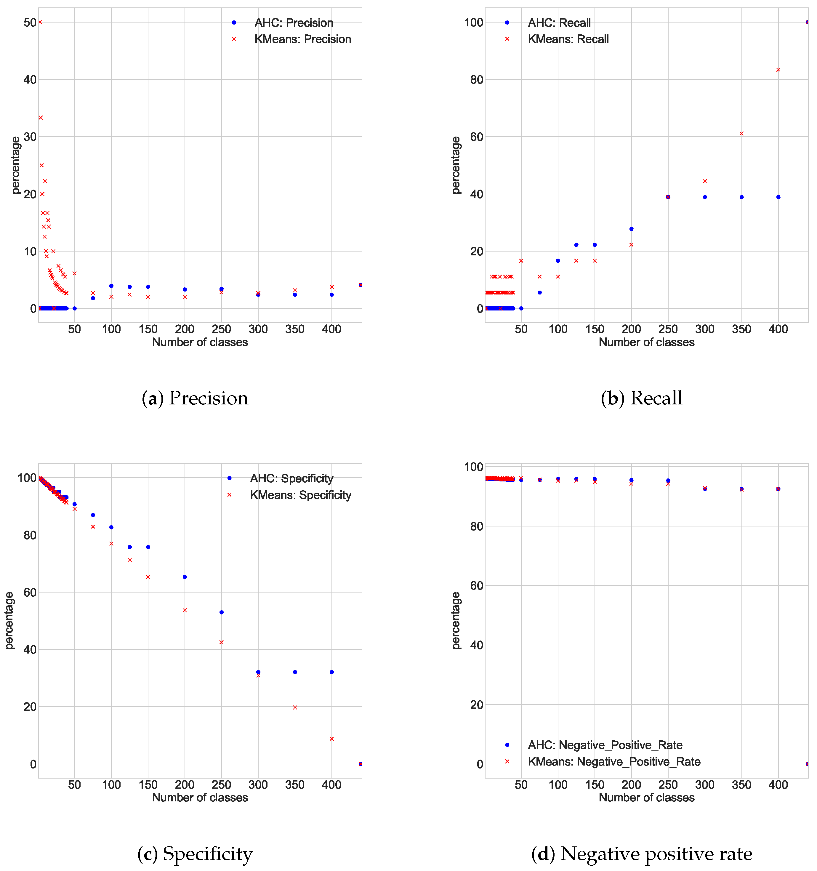
4.2. Comparison Between AHC and K-Means Performances

In this section, we carry out a comparative study of the two proposed classification algorithms: AHC and classification by K-means. As we mentioned in the methodology, our aim is to detect changes in road quality in a non-supervisory way, without specifying the nature of the change. The points of change subdivide the data into homogeneous consumptive classes. The algorithms are evaluated both according to several classic metrics (based on binary labeling) and according to a new metric that we consider relevant: the rate of agreement on the change. We are also interested in the experimental calculation time.

Figure 5 shows the experimental execution times for the K-means and AHC algorithms. Naturally, the fewer the classes, the longer the classification procedure. The times of the K-means algorithm largely dominate those of the AHC algorithm. This can be explained by the convergence process of the K-means algorithm, which is exploratory in nature. It was also predictable according to complexities of those algorithms that were polynomial for AHC and exponential for K-means.

Figure 6, Figure 7 and Figure 8 show the responses of the classification algorithms to the various usual confusion metrics as a function of the number of classes imposed. It should be noted that there are actually 19 classes and that fixing the number of classes (K) imposes the number of change points ($K-1$).

The accuracy rate (probability that an announced change will be effective) increases with the number of classes for the K-means algorithm. On the other hand, it increases with the number of classes for the AHC algorithm. However, the performances of the two algorithms stabilize in the middle zone ($2.5\%$ on average) for a relatively high number of classes compared to the actual number of classes. In fact, the more change points are proposed, the less likely it is that all these points really are change points. The average precision is $8.13\%$ for the K-means algorithm and $0.62\%$ for the AHC algorithm.

The recall rate (probability that a real change is detected) for the K-means and AHC algorithms is low for a small number of classes. It increases overall with the number of classes because, the more change point proposals there are, the more verifiable change points are included. The recall rate is on average $13.55\%$ for the K-means algorithm and $7\%$ for the AHC algorithm.

The specificity (probability that a point with no change will be considered as such) increases overall with the number of classes. It is on average $85.52\%$ for the K-means algorithm and $87.48\%$ for the AHC algorithm. The specificity decreases overall with the number of classes because the more change points are proposed, the greater the chances of proposing the wrong ones.

The true negative rate (the probability that a point considered to be without change really is) increases overall, although only slightly, with the number of classes. It is on average $93.73\%$ for the K-means algorithm and $93.6\%$ for the AHC algorithm. The decrease in the true negative rate can be explained by the fact that the fewer change point propositions there are, the fewer wrong propositions there are.

Overall, in terms of the confusion matrix, except for the specificity, the K-means algorithm seems to perform better than the AHC algorithm. We can extend the analysis through more synthetic indicators such as the F1-score, the agreement rate on change, the accuracy, the $\kappa$ coefficient, the Rand index and the adjusted Rand index. We use Figure 8 and Figure 9.

The F1-score is the harmonic mean between the accuracy and the recall rate. It therefore tries to strike a compromise between these two indicators, which must not be zero. Unsurprisingly, the average F1-score of the K-means algorithm ($6.38\%$) is higher than the average F1-score of the AHC algorithm ($1.11\%$). The value of the F1-score is better for a relatively small number of classes.

The rate of agreement on change (probability that the prognosis of change or not is endorsed) increases with the number of classes, since more class proposals expose unfounded considerations of change. The average F1-score is $3.32\%$ for the K-means algorithm and $0.57\%$ for the AHC algorithm. We note that the F1-score and the rate of agreement on the change have very similar appearances even if the ranges of values are not the same. On the one hand, this confirms the relevance of the F1-score and, on the other, validates the new metric of the rate of agreement with the change, which also offers better interpretation.

The accuracy (probability that a point is correctly considered) decreases significantly with the number of classes at least because the number of false positive increases. The average value is $82.59\%$ for the K-means algorithm and $84.18\%$ for the AHC algorithm.

The $\kappa$ coefficient has a very similar behavior with the accuracy. Its average value is $82.56\%$ for the K-means algorithm and $84.18\%$ for the AHC algorithm. This confirms the relevance of the accuracy offers better interpretation through in the context of clustering.

The Rand index (the probability that the prediction of whether or not two points in the siblings belong to the same class is correct) appears to be greater when the number of classes imposed is close to the actual number of classes. It is on average $82.84\%$ for the K-means algorithm and $86.33\%$ for the AHC algorithm.

The adjusted Rand index reveals that the AHC algorithm is more stable than the K-means algorithm. The former guarantees very often a performance better than the average of all possible performances while the K-means algorithm can be very below that average depending on the number of classes. The adjusted Rand index was in average $-64.36\%$ for the K-means algorithm and $8.84\%$ for the AHC algorithm.

Despite the low values of the F1-score and the rate of agreement on the change allow us to conclude that the exact detection of points of change is difficult. On the other hand, the relatively good performances of the accuracy and the Rand index show that the proposed algorithms do a good job of identifying homogeneous classes or phases. The AHC algorithm appears to offer a good compromise in terms of performance. This is in accordance with [19].

5. Conclusions

This work focused on detecting changes in the characteristics of roads along their route using a vehicle equipped with sensors such as accelerometer and GPS. The aim was to segment the geographical data collected by the sensors with a view to subsequent labeling that could be used to diagnose the state of the road. To do this, we used a dataset available via the url https://github.com/simonwu53/RoadSurfaceRecognition/blob/master/data/sensor_data_v2.zip (13 November 2024).

From the acceleration data available in the dataset, we determined trajectory curvatures. After an analysis of correlation and variance, we were able to identify the curvature that best explained the changes. Contrary to the usual considerations in the literature, vertical variations weakly explained these changes. This could be understood by the tendency of vehicle drivers to avoid obstacles. We then proposed two adapted algorithms: AHC and clustering by K-means. Performance was compared according to several metrics. By assimilating change detection to binary labeling, we were able to use the metrics derived from the confusion matrix (precision, recall, specificity, overall accuracy, and F1 score). Furthermore, since we are dealing with classification, we have also used some of the more common metrics in this field (Rand index, adjusted Rand index, statistical coefficient $\kappa$).

The results showed that curvature was a relevant characteristic for classifying road irregularities. The relative performance of the proposed algorithms varies from one metric to another. However, hierarchical ascending classification appears to be more stable in terms of performance and, above all, less costly in terms of computing time. This last observation could be very decisive for the needs of real-time evaluation of changes. The AHC algorithm appears to offer a good compromise in terms of performance. This is in accordance with our results discussed in Section 4, which show that AHC achieves faster computation times than K-means, albeit with slightly lower precision. This trade-off makes AHC particularly suitable for deployment in resource-constrained settings (e.g., mobile or embedded systems), where quick detection of irregularities may outweigh the need for high segmentation accuracy. Conversely, K-means remains preferable when precision is prioritized, such as in offline analysis or post-processing stages.

Although the proposed algorithms have demonstrated promising performance, several limitations must be acknowledged. A key limitation is that the number of clusters to be formed is not determined automatically, requiring manual intervention. In future work, we aim to address this by proposing features that remain constant per road segment, facilitating easier and more accurate label assignment, as suggested in [6]. One potential development involves introducing additional features that are consistent within each road segment. Such features could streamline the automatic labeling process and enhance the robustness of predictions. Furthermore, exploring advanced clustering techniques that dynamically determine the optimal number of clusters could significantly improve the adaptability and efficiency of algorithms. This work lays a foundation for future research focused on improving road safety and infrastructure maintenance through automated anomaly detection, with the potential to integrate real-time data processing and machine learning advancements for more scalable and accurate solutions.

References

1. Al-Sabaeei, A.M.; Souliman, M.I.; Jagadeesh, A. Smartphone applications for pavement condition monitoring: A review. Constr. Build. Mater. 2024, 410, 134207. [Google Scholar] [CrossRef]
2. Dhiman, A.; Klette, R. Pothole detection using computer vision and learning. IEEE Trans. Intell. Transp. Syst. 2019, 21, 3536–3550. [Google Scholar] [CrossRef]
3. Guan, J.; Yang, X.; Ding, L.; Cheng, X.; Lee, V.C.; Jin, C. Automated pixel-level pavement distress detection based on stereo vision and deep learning. Autom. Constr. 2021, 129, 103788. [Google Scholar] [CrossRef]
4. Rajamohan, D.; Gannu, B.; Rajan, K.S. MAARGHA: A prototype system for road condition and surface type estimation by fusing multi-sensor data. ISPRS Int. J. Geo-Inf. 2015, 4, 1225–1245. [Google Scholar] [CrossRef]
5. Anaissi, A.; Khoa, N.L.D.; Rakotoarivelo, T.; Alamdari, M.M.; Wang, Y. Smart pothole detection system using vehicle-mounted sensors and machine learning. J. Civ. Struct. Health Monit. 2019, 9, 91–102. [Google Scholar] [CrossRef]
6. Martinez-Ríos, E.A.; Bustamante-Bello, M.R.; Arce-Sáenz, L.A. A review of road surface anomaly detection and classification systems based on vibration-based techniques. Appl. Sci. 2022, 12, 9413. [Google Scholar] [CrossRef]
7. Seraj, F.; Zwaag, B.J.v.d.; Dilo, A.; Luarasi, T.; Havinga, P. RoADS: A road pavement monitoring system for anomaly detection using smart phones. In Big Data Analytics in the Social and Ubiquitous Context; Springer: Berlin/Heidelberg, Germany, 2015; pp. 128–146. [Google Scholar]
8. Sattar, S.; Li, S.; Chapman, M. Developing a near real-time road surface anomaly detection approach for road surface monitoring. Measurement 2021, 185, 109990. [Google Scholar] [CrossRef]
9. Boateng, F.G.; Klopp, J.M. Beyond bans. J. Transp. Land Use 2022, 15, 651–670. [Google Scholar] [CrossRef]
10. Egaji, O.A.; Evans, G.; Griffiths, M.G.; Islas, G. Real-time machine learning-based approach for pothole detection. Expert Syst. Appl. 2021, 184, 115562. [Google Scholar] [CrossRef]
11. Wu, S.; Hadachi, A. Road surface recognition based on deepsense neural network using accelerometer data. In Proceedings of the 2020 IEEE Intelligent Vehicles Symposium (IV), Las Vegas, NV, USA, 19 October–13 November 2020; pp. 305–312. [Google Scholar]
12. Amarbayasgalan, T.; Pham, V.H.; Theera-Umpon, N.; Ryu, K.H. Unsupervised anomaly detection approach for time-series in multi-domains using deep reconstruction error. Symmetry 2020, 12, 1251. [Google Scholar] [CrossRef]
13. Aminikhanghahi, S.; Cook, D.J. A survey of methods for time series change point detection. Knowl. Inf. Syst. 2017, 51, 339–367. [Google Scholar] [CrossRef] [PubMed]
14. Benevento, A.; Durante, F. Correlation-based hierarchical clustering of time series with spatial constraints. Spat. Stat. 2024, 59, 100797. [Google Scholar] [CrossRef]
15. Tran, D.H. Automated change detection and reactive clustering in multivariate streaming data. In Proceedings of the 2019 IEEE-RIVF International Conference on Computing and Communication Technologies (RIVF), Danang, Vietnam, 20–22 March 2019; pp. 1–6. [Google Scholar]
16. Bezdan, T.; Stoean, C.; Naamany, A.A.; Bacanin, N.; Rashid, T.A.; Zivkovic, M.; Venkatachalam, K. Hybrid fruit-fly optimization algorithm with k-means for text document clustering. Mathematics 2021, 9, 1929. [Google Scholar] [CrossRef]
17. Javed, A.; Lee, B.S.; Rizzo, D.M. A benchmark study on time series clustering. Mach. Learn. Appl. 2020, 1, 100001. [Google Scholar] [CrossRef]
18. Holder, C.; Middlehurst, M.; Bagnall, A. A review and evaluation of elastic distance functions for time series clustering. Knowl. Inf. Syst. 2024, 66, 765–809. [Google Scholar] [CrossRef]
19. Keogh, E.; Chu, S.; Hart, D.; Pazzani, M. An online algorithm for segmenting time series. In Proceedings of the 2001 IEEE International Conference on Data Mining, San Jose, CA, USA, 29 November–2 December 2001; pp. 289–296. [Google Scholar]
20. Basavaraju, A.; Du, J.; Zhou, F.; Ji, J. A machine learning approach to road surface anomaly assessment using smartphone sensors. IEEE Sens. J. 2019, 20, 2635–2647. [Google Scholar] [CrossRef]
21. Nguyen, V.K.; Renault, É.; Milocco, R. Environment monitoring for anomaly detection system using smartphones. Sensors 2019, 19, 3834. [Google Scholar] [CrossRef]
22. Wu, C.; Wang, Z.; Hu, S.; Lepine, J.; Na, X.; Ainalis, D.; Stettler, M. An automated machine-learning approach for road pothole detection using smartphone sensor data. Sensors 2020, 20, 5564. [Google Scholar] [CrossRef]
23. Rajput, P.; Chaturvedi, M.; Patel, V. Road condition monitoring using unsupervised learning based bus trajectory processing. Multimodal Transp. 2022, 1, 100041. [Google Scholar] [CrossRef]
24. Bustamante-Bello, R.; García-Barba, A.; Arce-Saenz, L.A.; Curiel-Ramirez, L.A.; Izquierdo-Reyes, J.; Ramirez-Mendoza, R.A. Visualizing street pavement anomalies through fog computing v2i networks and machine learning. Sensors 2022, 22, 456. [Google Scholar] [CrossRef]
25. Kim, G.; Kim, S. A road defect detection system using smartphones. Sensors 2024, 24, 2099. [Google Scholar] [CrossRef] [PubMed]
26. He, D.; Shi, Q.; Xue, J.; Atkinson, P.M.; Liu, X. Very fine spatial resolution urban land cover mapping using an explicable sub-pixel mapping network based on learnable spatial correlation. Remote Sens. Environ. 2023, 299, 113884. [Google Scholar] [CrossRef]
27. van Kuppevelt, D.; Heywood, J.; Hamer, M.; Sabia, S.; Fitzsimons, E.; van Hees, V. Segmenting accelerometer data from daily life with unsupervised machine learning. PLoS ONE 2019, 14, e0208692. [Google Scholar] [CrossRef]
28. Etemad, M.; Júnior, A.S.; Hoseyni, A.; Rose, J.; Matwin, S. A Trajectory Segmentation Algorithm Based on Interpolation-based Change Detection Strategies. In Proceedings of the EDBT/ICDT Workshops, Lisbon, Portugal, 26 March 2019; p. 58. [Google Scholar]
29. Tapia, G.; Colomé, A.; Torras, C. Unsupervised Trajectory Segmentation and Gesture Recognition through Curvature Analysis and the Levenshtein Distance. In Proceedings of the 2024 7th Iberian Robotics Conference (ROBOT), Madrid, Spain, 6–8 November 2024; pp. 1–8. [Google Scholar]
30. Chilov, G. Fonctions d’une Variable [Tome 1], 1ère er 2eme Parties; Mir: Moscou, Russie, 1973. [Google Scholar]
31. Fortin, A. Analyse Numérique pour Ingénieurs; Presses Inter Polytechnique: Montréal, QC, Canada, 2011. [Google Scholar]
32. Saporta, G. Probabilités, Analyse des Données et Statistique; Editions Technip: Paris, France, 2006. [Google Scholar]
33. Rand, W.M. Objective criteria for the evaluation of clustering methods. J. Am. Stat. Assoc. 1971, 66, 846–850. [Google Scholar] [CrossRef]
34. Hubert, L.; Arabie, P. Comparing partitions. J. Classif. 1985, 2, 193–218. [Google Scholar] [CrossRef]
35. Zhang, H.; Ho, T.B.; Zhang, Y.; Lin, M.S. Unsupervised feature extraction for time series clustering using orthogonal wavelet transform. Informatica 2006, 30, 305–319. [Google Scholar]
36. Gates, A.J.; Ahn, Y.Y. The impact of random models on clustering similarity. J. Mach. Learn. Res. 2017, 18, 1–28. [Google Scholar]
37. Zheng, Z.; Zhou, M.; Chen, Y.; Huo, M.; Sun, L. QDetect: Time series querying based road anomaly detection. IEEE Access 2020, 8, 98974–98985. [Google Scholar] [CrossRef]
38. Zheng, Z.; Zhou, M.; Chen, Y.; Huo, M.; Sun, L.; Zhao, S.; Chen, D. A fused method of machine learning and dynamic time warping for road anomalies detection. IEEE Trans. Intell. Transp. Syst. 2020, 23, 827–839. [Google Scholar] [CrossRef]
Figure 1. Overall methodological framework.
Mathematics 13 01921 g001
Figure 2. Acceleration as function of the length of the path.
Mathematics 13 01921 g002
Figure 3. Curvature as function of the length of the path.
Mathematics 13 01921 g003
Figure 4. Correlation analysis.
Mathematics 13 01921 g004
Figure 5. Distributions of the computational time.
Mathematics 13 01921 g005
Figure 6. Confusion matrix as function of the number of classes.
Mathematics 13 01921 g006
Figure 7. Distributions of the confusion metrics.
Mathematics 13 01921 g007
Figure 8. Global metrics as function of the number of classes.
Mathematics 13 01921 g008
Figure 9. Distributions of the global metrics.
Mathematics 13 01921 g009