A Cloud-Edge-End Collaboration Framework for Fixed-Time Distributed Optimization of Virtual Power Plants

Abstract

As the power grid expands, concerns about system computation speed and information privacy are becoming more critical. While distributed optimization methods protect individual privacy effectively, they struggle with computational efficiency in complex topologies. To address these issues, this paper proposes a cloud–edge–end collaboration framework consisting of a cloud server and multiple edge servers. This framework enables parallel computation of multiple distributed optimization algorithms. Additionally, a distributed fixed-time optimization consensus algorithm is designed for virtual power plants, allowing the convergence time to be predetermined offline. The fixed-time convergence of the algorithm is proven and its effectiveness and superiority are demonstrated through simulation cases.

1. Introduction

As the proportion of renewable energy sources increases, the volatility and stochasticity of their output present significant challenges to the stable operation of power systems [1]. Concurrently, energy storage devices, flexible loads, and distributed energy power plants at the distribution network level heighten the uncertainty of demand-side electricity consumption. Power dispatch plays a crucial role in enhancing the grid integration of renewable energy sources and ensuring stable power system operation [2].

The concept of the virtual power plant (VPP) was introduced to accommodate renewable energy sources more efficiently [3], with its primary function being participation in the grid’s overall power scheduling. A VPP leverages advanced communication, measurement, regulation, and control technologies to aggregate extensive user-side resources such as flexible loads, distributed power sources, and distributed energy storage [4]. By integrating various distributed energy resources, the VPP is managed and dispatched through the dispatch center to address the economic dispatch problem of the power grid [5]. Thus, studying the economic scheduling of VPPs is of great practical significance for resolving the challenges of large-scale renewable energy grid integration.

The traditional economic dispatch problem for a VPP is usually solved using a centralized control framework [6]. The centralized algorithm is characterized by the inclusion of a central controller, which collects information from all sensors and performs calculations. The corresponding commands are then fed back to each local actuator. The centralized algorithm is easy to implement and convenient to control. However, there are still a number of problems [7]. First, the control center is in control of the whole VPP; if it fails, this will lead to control failure of the whole system, which represents a major hidden danger to the stable operation of VPP and leads to low system reliability. Second, with an increasing number of distributed energy sources, the amount of information that the control center needs to collect and process gradually increases, leading to a significant reduction in the operational efficiency of the microgrid; at the same time, the resulting gradual increase in two-way communication links leads to high construction costs of the communication network. Third, the centralized algorithm needs to collect information from all units, resulting in less privacy for independent individuals.

In contrast to a centralized framework, a distributed framework operates in a decentralized manner. Instead of relying on a central controller, this approach uses local controllers distributed among local agents that interact with each other. In a virtual power plant (VPP), the generation unit, load unit, and energy storage unit function as independent agents [8]. Each agent collaborates to achieve the global objectives of the VPP through local communication with neighboring agents. This model’s advantage lies in achieving global control objectives solely through local control and information exchange [9]. The decentralized approach significantly reduces the construction cost of communication, enhances the overall reliability and flexibility of the VPP, and effectively addresses the shortcomings of centralized algorithms [10].

Due to the numerous advantages of distributed frameworks, related optimization problems have garnered increasing attention in recent years [11,12,13]. In [14], a consensus algorithm was proposed in which each generating unit iteratively updates its state information by interacting with neighboring generating units, eventually converging to the optimal solution. In [15], a distributed augmented power flow algorithm for networked microgrids was designed incorporating Newton-type power flow considerations. In [16], a novel distributed approach was introduced to manage the energy of microgrids with the aim of maximizing social welfare.

In the economic dispatch problem of VPPs, the intermittency and uncertainty of renewable energy sources necessitate the design of economic dispatch algorithms with fast convergence in order to meet system dispatch requirements; hence, designing distributed optimization algorithms with fast convergence is crucial. Fast convergence differs from traditional asymptotic convergence methods such as exponential, finite-time, and fixed-time optimization [17,18]. In [19], a distributed consistency protocol with an exponential convergence rate was developed based on the theory of exponential stability. Unlike asymptotic convergence, this protocol was assigned a specific convergence rate, satisfying the property of exponential convergence. In [20], a finite-time consensus was designed based on the overall cost function in order to accelerate the algorithm’s convergence rate. In [21], a fixed-time distributed optimization algorithm based on an event-triggered strategy was proposed to solve optimization problems in multi-agent systems with consistency constraints and strongly convex local cost functions. In [22], a consensus of multi-agent systems was applied to the optimal control of microgrids, employing a finite-time consensus algorithm to enhance convergence speed and control accuracy. In [23], a novel momentum-based distributed iterative algorithm was proposed to address resource allocation and scheduling problems. This algorithm ensures the feasibility and fast convergence of the solution in the presence of nonlinear coupling constraints and delays.

Although the distributed optimization algorithms mentioned above improve the convergence rate, their convergence time depends on the initial state of the agents. This dependency means that the convergence time cannot be predetermined offline. To address this limitation, the concept of fixed-time stability was introduced [24]. Algorithms based on fixed-time stabilization ensure that the state converges to the optimal solution within a fixed time, which can be set in advance according to task requirements. However, fixed-time consensus has not been extensively studied in the context of economic scheduling problems in VPPs, necessitating further research.

As the scale of actual power systems increases, distributed framework algorithms struggle to accommodate complex network topologies [25]. To address this challenge, this paper introduces the concept of a cloud–edge–end cooperative control framework. First, the power grid is divided into multiple regions based on the network topology. Each region is then equipped with an edge server for control. All edge servers are connected to a cloud server, which utilizes its computational resources to calculate the power output required from each region. The cloud server then sends the computation results to each edge server, which further enables each agent to reach a consensus through a distributed optimization algorithm. Consequently, the distributed optimization algorithm designed under the cloud–edge–end framework is better able to meet the demands of modern power systems. The contributions of this paper are as follows:

(1)

A fixed-time consensus optimization algorithm is proposed to address the economic scheduling problem of VPPs. Unlike the approach in [20], the proposed algorithm not only exhibits a high convergence rate but also avoids dependence on the system’s initial values. In addition, it can be designed offline. Compared to [22], the proposed optimization algorithm incorporates more constraints, reflecting the actual conditions of the grid. Therefore, the algorithm presented in this paper is more practically significant.

(2)

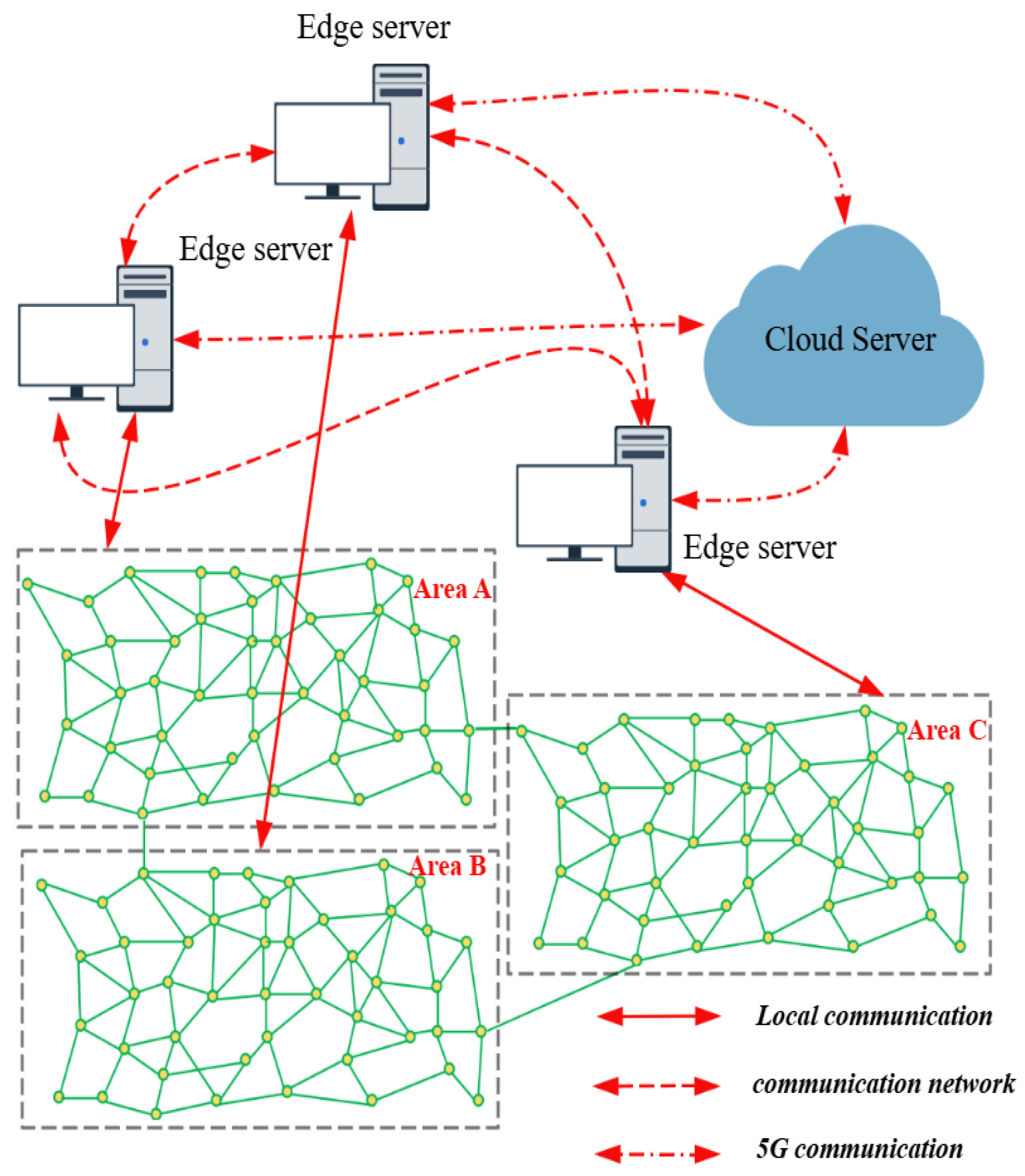
A framework for cloud–edge–end collaborative control is proposed. Compared to the centralized framework [5], the proposed cloud–edge–end collaboration framework better protects user privacy, as the cloud server only requires aggregated regional information rather than individual agent data to solve the problem. At the edge server level, each agent only needs to exchange gradients with neighboring agents. Unlike the distributed framework [21], the cloud–edge–end collaboration framework allows for parallel computation of multiple distributed optimization algorithms, enhancing the speed of solving optimization problems.

The remainder of this paper is organized as follows: Section 2 presents the VPP model and the cloud–edge–end cooperative control framework along with a description of the economic scheduling problem of VPPs; in Section 3, a distributed fixed-time optimized consensus algorithm is designed and its convergence is proven; Section 4 verifies the effectiveness of the algorithm through a simulation case; finally, conclusions are provided in Section 5.

2. Model and Preliminaries

2.1. VPP Cyber–Physical System Model

A cyber–physical system (CPS) is an advanced engineering system that integrates computation, communication, and control. The CPS approach has been widely adopted in power systems. Figure 1 illustrates the cyber–physical system model of a VPP. In this model, power generation devices, energy storage devices, and loads constitute the physical layer of the CPS. Each device is equipped with an agent; the communication network between these agents forms the information layer of the CPS. This paper introduces graph theory to describe the information–physical system model of the VPP. The topology of the VPP can be represented by a binary group $\mathcal{G}=\{\mathcal{V},\mathcal{E}\}$, where $\mathcal{V}$ denotes a set of nodes, each representing an agent, and $\mathcal{E}$ denotes the set of edges. The adjacency matrix $A=\left[a_{ij}\right]$ is defined such that $a_{ij}=1$ if node i and node j communicate with each other and $a_{ij}=0$ otherwise.

2.2. Cloud–Edge–End Collaboration Framework for VPPs

Traditional power allocation models employ centralized coordination, with generation facilities sharing their operational metrics with a central controller in order to determine capacity distribution according to grid demand. Although systematic, such approaches exhibit critical weaknesses including fragile adaptability to operational uncertainties and compromised confidentiality of proprietary technical data.

The current distributed economic dispatch framework treats each unit as an independent agent. Each agent exchanges only partial information with neighboring agents while optimizing its own problem to achieve coordinated system optimization. Although the distributed economic dispatch method can ensure system privacy and robustness, the overall calculation speed significantly decreases as the interconnected system grows larger.

To address these shortcomings, this paper proposes a cloud–edge–end collaboration framework for economic dispatch, as shown in Figure 2. The hierarchical implementation commences with sectoral partitioning of the power network into three operational zones (A, B, C). At the cloud computing tier, demand forecasting algorithms combined with inter-zone structural analysis enable derivation of optimal generation quotas through constrained optimization techniques. In the second step, each zone (A, B, C) is equipped with an edge server. Subsequently, distributed edge computing nodes deploy agent-based modeling for intra-zone coordination, where generation facilities autonomously negotiate power outputs through neighbor-aware communication protocols while preserving operational confidentiality.

2.3. VPP Supply–Demand Model

The VPP components are power generation, battery energy storage, basic load, and controllable load.

(1)

Power Generation Unit

The cost function of the generation set is

$$\begin{array}{c}\hfill f_i^w\left(p_i^w\right)=a_i^w{\left(p_i^w\right)}^2+b_i^w{p}_i^w+c_i^w,\end{array}$$

(1)

where $a_i^w,b_i^w,c_i^w$ are the cost coefficients of the ith generator, $i=1,2,\dots ,n_w$. In practice, cost functions are derived through curve fitting based on the data obtained from heat rate tests or from the plant’s design engineers; thus, non-quadratic functions may be used for better fitting performance.

(2)

Power Controllable Load

The controllable load reduction cost function is

$$\begin{array}{c}\hfill f_i^u\left(p_i^u\right)=a_i^u{\left(p_i^u\right)}^2+b_i^u{p}_i^u+c_i^u,\end{array}$$

(2)

where $a_i^u,b_i^u$ and $c_i^u$ are non-negative cost factors, $i=1,2,\dots ,n_u$.

(3)

Battery Energy Storage

Due to the battery internal resistance, the internal power loss of the BESSs cannot be neglected. The cost function for the battery energy storage cost can be modeled as follows:

$$\begin{array}{c}\hfill f_i^s\left(p_i^s\right)=a_i^s{\left(p_i^s\right)}^2+b_i^s{p}_i^s+c_i^s\end{array}$$

(3)

where $a_i^s,b_i^s$ and $c_i^s$ are non-negative cost factors, $p_i^s$ denotes charge or discharge power, and $i=1,2,\dots ,n_s$.

The charge and discharge state of the battery energy storage system must be limited to a certain range in order to avoid overcharge or discharge:

$$\begin{array}{cc}\hfill & {SoC}_i\left(\eta \right)={SoC}_i(\eta -1)+{\displaystyle \frac{p_i^s{\vartheta }_i{\Gamma }_i}{B_i}},\hfill \\ \hfill & {SoC}_i^{\min }\left(\eta \right)⩽{SoC}_i\left(\eta \right)⩽{SoC}_i^{\max }\left(\eta \right),\hfill \end{array}$$

(4)

where ${SoC}_i\left(\eta \right)$ is the current charge of the battery energy storage of the i th storage at time $\eta$, ${\Gamma }_i$ is the charging or discharging time, $B_i$ is the capacity of the battery, ${\vartheta }_i$ is the charging or discharging efficiency.

(4)

Power balance and flow constraint

The active power balance constraint at node i is as follow

$$\begin{array}{c}{\displaystyle \sum _{j\in N}}{P}_{ji}-{\displaystyle \sum _{k\in N}}{P}_{ik}={\displaystyle \sum _{j\in N}}{B}_{ji}\left({\theta }_j-{\theta }_i\right)-{\displaystyle \sum _{k\in N}}{B}_{ik}\left({\theta }_i-{\theta }_k\right),\\ P_i-{\displaystyle \sum _{k\in N}}{P}_{ik}+{\displaystyle \sum _{j\in N}}{P}_{ji}=0,\end{array}$$

(5)

where $P_{ji}$ and $P_{ik}$ denote the active power input and output of energy hub i, $N_i^f$ represents the set of nodes neighboring node i, and $N=n_w+n_u+n_s$. In addition, $B_{ji}$ and $B_{ik}$ mean the conductance of line $ji$ and line $ik$, while ${\theta }_i$, ${\theta }_j$, and ${\theta }_k$ denote the phase angles of nodes i, j, and k, respectively, and $P_i$ expresses the active power generated by node i.

The VPP should satisfy the power balance

$$\begin{array}{c}\hfill \sum _{i=1}^{nw}{p}_i^w+\sum _{i=1}^{ns}{p}_i^s=P_l-\sum _{i=1}^{nu}{p}_i^u,\end{array}$$

(6)

where $P_l$ is considered as the constant load.

(5)

Problem Description

The optimization objective of this stage is to minimize the overall expected operating cost while satisfying the power supply and demand balance and the power limitation of each unit. It is described by the following time-varying optimization problem:

$$\begin{array}{cc}\hfill min& \sum _{T=1}^{T_{\mathrm{sum}}}\left(\sum _{i=1}^{n_w}{f}_i^w\left(p_i^w\right)+\sum _{i=1}^{n_u}{f}_i^u\left(p_i^u\right)+\sum _{i=1}^{n_s}{f}_i^s\left(p_i^s\right)\right)\hfill \\ \hfill \mathrm{s}.\mathrm{t}.& \sum _{i=1}^{nw}{p}_i^w+\sum _{i=1}^{ns}{p}_i^s=P_l-\sum _{i=1}^{n_u}{p}_i^u\hfill \\ \hfill & p_{i,min}^w\le \left|p_i^w\right|⩽p_{i,max}^w\hfill \\ \hfill & p_{i,min}^u\le \left|p_i^u\right|⩽p_{i,max}^u\hfill \\ \hfill & p_{i,min}^s\le \left|p_i^s\right|⩽p_{i,max}^s\hfill \\ \hfill & \mathrm{and}\left(5\right),\hfill \end{array}$$

(7)

where $p_{i,min}^w$, $p_{i,min}^u$, and $p_{i,min}^s$ denote the minimum power of each power unit, $p_{i,max}^w$, $p_{i,max}^u$, and $p_{i,max}^s$ indicate the maximum power of each power unit, T means a time node (commonly defined as an hour), and $T_{\mathrm{sum}}$ represents the number of time nodes.

Assumption 1.

The communication topology of a microgrid can be described by a graph $\mathcal{G}$ which is undirected and connected.

2.4. Definition and Some Lemmas

Consider the differential system

$$\begin{array}{c}\hfill \dot{y}=g(t,y),y\left(t_0\right)=y_0,\end{array}$$

(8)

where $t_0$ is the initial time, $y\in {\mathbb{R}}^N$ is the system state, and $g(t,y)$ is a nonlinear function. The solution $\zeta (t,y_0)$ of (8) is interpreted in the Filippov sense, with $y=0$ being the unique equilibrium.

Definition 1.

System (8) is said to be fixed-time stable if there exists a settling time $\mathcal{T}\left(y_0\right)$ such that ${lim}_{t\to T\left(y_0\right)}\zeta (t,y_0)=0$ and $\zeta (t,y_0)=0$ for $\forall t\ge \mathcal{T}\left(y_0\right)$ and if there additionally exists a ${\mathcal{T}}_{max}>0$ such that $\mathcal{T}\left(y_0\right)<{\mathcal{T}}_{max}$, $\forall y_0\in {\mathbb{R}}^N$.

Lemma 1

([26]). If ${\xi }_1,{\xi }_2,\dots ,{\xi }_N⩾0$, then

$$\begin{array}{cc}\hfill & {\left(\sum _{i=1}^N{\xi }_i\right)}^b<\sum _{i=1}^N{\xi }_i^b<N^{1-b}{\left(\sum _{i=1}^N{\xi }_i\right)}^b,if0<b<1,\hfill \\ \hfill & N^{1-b}{\left(\sum _{i=1}^N{\xi }_i\right)}^b<\sum _{i=1}^N{\xi }_i^b,if1<b<\infty .\hfill \end{array}$$

(9)

Lemma 2

([27]). Given a differential system $\dot{y}=g(t,y)$, if there exists a positive-definite Lyapunov function $V\left(y\right)$ such that

$$\begin{array}{c}\hfill \dot{V}\left(y\right)⩽-\alpha V^p\left(y\right)-\beta V^q\left(y\right)\end{array}$$

(10)

where $\alpha >0,\beta >0,p=1-{\displaystyle \frac{1}{2\mu }},q=1+{\displaystyle \frac{1}{2\mu }},\mu >1$, then the origin is fixed-time stable for the considered system with the settling time estimated as

$$\begin{array}{c}\hfill \mathcal{T}\left(y_0\right)⩽{\mathcal{T}}_{max}={\displaystyle \frac{\pi \mu }{\sqrt{\alpha \beta }}}.\end{array}$$

(11)

Lemma 3

([28]). For any non-empty closed convex set Ω and $y\in {\mathbb{R}}^N,∥P_{\Omega }\left(y\right)-y∥$ is continuous on y and $\nabla \left({∥P_{\Omega }\left(y\right)-y∥}^2\right)=-2\left(P_{\Omega }\left(y\right)-y\right)$, where $\nabla (·)$ is the gradient of $(·)$.

3. Main Results

3.1. Consensus Algorithm Design

If the optimal cost is satisfied at each time $\tau$, then the total cost is the optimal solution. Therefore, the optimization problem at time $\tau$ can be described as follows:

$$\begin{array}{cc}\hfill min& f(x,T)=\sum _{i=1}^N{f}_i\left(x_i,T\right)\hfill \\ \hfill \mathrm{s}.\mathrm{t}.& \sum _{i=1}^N{x}_i=\sum _{i=1}^N{d}_i\hfill \\ \hfill & x_i\in \Omega \hfill \end{array}$$

(12)

where $f(x,\tau )$ means the sum of all equipment costs at time T, $x_i$ represents the generation power, N denotes the number of agents, $d_i$ signifies the load power, and $\Omega$ indicates the set of linear inequality constraints defined in (7).

The whole system is considered as a multi-agent system, in which the topology of the system can be represented by an undirected graph $\mathcal{G}$. The distributed algorithm designed by each agent can be described as follows:

$$\begin{array}{cc}\hfill {\dot{x}}_i=& u_i,\hfill \\ \hfill u_i=& {\phi }_i+\left|{\phi }_i\right|sign\left(P_{\Omega }\left(x_i\right)-x_i\right)+k_1{\left(P_{\Omega }\left(x_i\right)-x_i\right)}^{\left[a\right]}\hfill \\ \hfill & +k_2{\left(P_{\Omega }\left(x_i\right)-x_i\right)}^{\left[b\right]},\hfill \\ \hfill {\phi }_i=& -m_1{e}_i^{\left[a\right]}-m_2{e}_i^{\left[b\right]}+\sum _{j=1}^N{a}_{ij}{\left(\nabla f_j\left(x_j\right)-\nabla f_i\left(x_i\right)\right)}^{\left[a\right]}\hfill \\ \hfill & +\sum _{j=1}^N{a}_{ij}{\left(\nabla f_j\left(x_j\right)-\nabla f_i\left(x_i\right)\right)}^{\left[b\right]},\hfill \\ \hfill e_i=& x_i-d_i-{\int }_0^t\sum _{j=1}^N{a}_{ij}{\left(\nabla f_j\left(x_j\left(\tau \right)\right)-\nabla f_i\left(x_i\left(\tau \right)\right)\right)}^{\left[a\right]}\mathrm{d}\tau \hfill \\ \hfill & -{\int }_0^t\sum _{j=1}^N{a}_{ij}{\left(\nabla f_j\left(x_j\left(\tau \right)\right)-\nabla f_i\left(x_i\left(\tau \right)\right)\right)}^{\left[b\right]}\mathrm{d}\tau \hfill \end{array}$$

(13)

where $u_i$ is designed to obtain an optimal solution in a fixed time, $e_i$ is designed to achieve total load demand constraints, ${\phi }_i$ is designed to drive the state $x_i$ approach to the optimal value, $k_1$, $k_2$, $m_1$, $m_2$ are positive constants, $0<a<1$, $b>1$, $a+b=2$, and $x^{\left[k\right]}=sign\left(x\right){\left|x\right|}^k$.

In the cloud–edge–end cooperative control framework, the power generation in each region is first solved at the level of the cloud. Next, a distributed consensus algorithm is applied to each region. Figure 3 delineates the convergence protocol governing collaborative decision-making among distributed autonomous entities and provides a systematic presentation of the specific operational stages.

Step 1. Input the topology and the predicted load value, then let the iteration step $k=0$.

Step 2. Renew the consensus variables of the agent using the exchange gradient.

Step 3. Calculate the update value $x_i(k+1)$ for each agent.

Step 4. Calculate the power deviation ${\sum }_{i=1}^N{x}_i(k+1)-{\sum }_{i=1}^N{d}_i$

Step 5. Adhere to computational accuracy thresholds. If ${\sum }_{i=1}^N{x}_i(k+1)-{\sum }_{i=1}^N{d}_i=0$, then the real power mismatch falls within the permissible tolerance, triggering termination of the recursive computation process. If ${\sum }_{i=1}^N{x}_i(k+1)-{\sum }_{i=1}^N{d}_i=0$, then set the iteration steps $k=k+1$ and return to Step 2.

3.2. Consensus Analysis

Theorem 1.

For the system in (13), it is possible to achieve fixed-time consensus.

Proof. 

Consider the Lyapunov function

$$\begin{array}{cc}\hfill & V_{1,i}={\displaystyle \frac{1}{2}}{\left(P_{\Omega }\left(x_i\right)-x_i\right)}^2,\forall i\in {\rm Y}=\{1,\dots ,N\},\hfill \\ \hfill & V_{2,i}={\displaystyle \frac{1}{2}}{e}_i^2,\forall i\in {\rm Y},\hfill \\ \hfill & V_3\left(\mathbf{x}\right)=f\left(\mathbf{x}\right)-f\left({\mathbf{x}}^{*}\right),\hfill \end{array}$$

(14)

where $\mathbf{x}={\left[x_1,\dots ,x_N\right]}^T$, ${\mathbf{x}}^{*}$ denotes the optimal solution for convergence of $\mathbf{x}$.

Step 1.

$$\begin{array}{c}\hfill V_{1,i}={\displaystyle \frac{1}{2}}{\left(P_{\Omega }\left(x_i\right)-x_i\right)}^2,\forall i\in {\rm Y}.\end{array}$$

(15)

Then, we obtain the derivative of $V_{1,i}$:

$$\begin{array}{cc}\hfill {\dot{V}}_{1,i}=& -\left(P_{\Omega }\left(x_i\right)-x_i\right){\dot{x}}_i\hfill \\ \hfill =& -\left(P_{\Omega }\left(x_i\right)-x_i\right)\left({\phi }_i+\left|{\phi }_i\right|sign\left(P_{\Omega }\left(x_i\right)-x_i\right)\right)\hfill \\ \hfill & -k_1{\left|P_{\Omega }\left(x_i\right)-x_i\right|}^{a+1}-k_2{\left|P_{\Omega }\left(x_i\right)-x_i\right|}^{b+1}.\hfill \end{array}$$

(16)

According to ${\phi }_i\left(P_{\Omega }\left(x_i\right)-x_i\right)-\left|{\phi }_i\right|\left|P_{\Omega }\left(x_i\right)-x_i\right|⩽0$, we have

$$\begin{array}{cc}\hfill {\dot{V}}_{1,i}& ⩽-k_1{\left({\left(P_{\Omega }\left(x_i\right)-x_i\right)}^2\right)}^{{\displaystyle \frac{a+1}{2}}}-k_2{\left({\left(P_{\Omega }\left(x_i\right)-x_i\right)}^2\right)}^{{\displaystyle \frac{b+1}{2}}}\hfill \\ \hfill & =-k_1{\left(2V_{1,i}\right)}^{{\displaystyle \frac{a+1}{2}}}-k_2{\left(2V_{2,i}\right)}^{{\displaystyle \frac{b+1}{2}}}\hfill \\ \hfill & =-2^{{\displaystyle \frac{a+1}{2}}}{k}_1{\left(V_{1,i}\right)}^{{\displaystyle \frac{a+1}{2}}}-2^{{\displaystyle \frac{b+1}{2}}}{k}_2{\left(V_{1,i}\right)}^{{\displaystyle \frac{b+1}{2}}}.\hfill \end{array}$$

(17)

Similarly, there exists a fixed time ${\mathcal{T}}_1>0$ such that ${lim}_{t\to {\mathcal{T}}_1}{V}_{1,i}=0$, and ${\mathcal{T}}_1$ is estimated by

$$\begin{array}{c}\hfill {\mathcal{T}}_1⩽{\displaystyle \frac{\pi 2^{\frac{2-(a+b)}{4}}}{(b-a)\sqrt{k_1{k}_2}}}.\end{array}$$

(18)

Therefore, it is concluded that $x_i$ enter ${\Omega }_i$ in a limited time.

Step 2. As $\mathrm{t}⩾{\mathcal{T}}_1$, it yields

$$\begin{array}{cc}\hfill {\dot{x}}_i=& -m_1{e}_i^{\left[a\right]}-m_2{e}_i^{\left[b\right]}+\sum _{j=1}^N{a}_{ij}{\left(\nabla f_j\left(x_j\right)-\nabla f_i\left(x_i\right)\right)}^{\left[a\right]}\hfill \\ \hfill & +\sum _{j=1}^N{a}_{ij}{\left(\nabla f_j\left(x_j\right)-\nabla f_i\left(x_i\right)\right)}^{\left[b\right]}.\hfill \end{array}$$

(19)

Consider the following Lyapunov function:

$$\begin{array}{c}\hfill V_{2,i}={\displaystyle \frac{1}{2}}{e}_i^2,\forall i\in {\rm Y}.\end{array}$$

(20)

In addition we can obtain the derivative of $V_{2,i}$ considering Equation (19) as follows:

$$\begin{array}{cc}\hfill {\dot{V}}_{2,i}& =e_i{\dot{e}}_i\hfill \\ \hfill & =e_i\left(-m_1{e}_i^{\left[a\right]}-m_2{e}_i^{\left[b\right]}\right)\hfill \\ \hfill & =-m_1{\left(2V_{2,i}\right)}^{{\displaystyle \frac{a+1}{2}}}-m_2{\left(2V_{2,i}\right)}^{{\displaystyle \frac{b+1}{2}}}\hfill \\ \hfill & =-2^{{\displaystyle \frac{a+1}{2}}}{m}_1{\left(V_{2,i}\right)}^{{\displaystyle \frac{a+1}{2}}}-2^{{\displaystyle \frac{b+1}{2}}}{m}_2{\left(V_{2,i}\right)}^{{\displaystyle \frac{b+1}{2}}}.\hfill \end{array}$$

(21)

In view of Lemma 2, there exists a fixed time ${\mathcal{T}}_2>0$ such that ${lim}_{t\to {\mathcal{T}}_2}{V}_{2,i}=0$ and ${\mathcal{T}}_2$ is estimated by

$$\begin{array}{c}\hfill {\mathcal{T}}_2⩽{\mathcal{T}}_1+{\displaystyle \frac{\pi 2^{\frac{2-(a+b)}{4}}}{(b-a)\sqrt{m_1{m}_2}}}.\end{array}$$

(22)

Based on $V_{3,i}=0$ and Equation (13), it follows that

$$\begin{array}{cc}\hfill e_i=& x_i-d_i-{\int }_0^t\sum _{j=1}^N{a}_{ij}{\left(\nabla f_j\left(x_j\left(\tau \right)\right)-\nabla f_i\left(x_i\left(\tau \right)\right)\right)}^{\left[a\right]}\mathrm{d}\tau \hfill \\ \hfill & -{\int }_0^t\sum _{j=1}^N{a}_{ij}{\left(\nabla f_j\left(x_j\left(\tau \right)\right)-\nabla f_i\left(x_i\left(\tau \right)\right)\right)}^{\left[b\right]}\mathrm{d}\tau =0.\hfill \end{array}$$

(23)

Thus,

$$\begin{array}{cc}\hfill \sum _{i=1}^N{e}_i=& \sum _{i=1}^N{x}_i-\sum _{i=1}^N{d}_i\hfill \\ \hfill & -\sum _{i=1}^N{\int }_0^t\sum _{j=1}^N{a}_{ij}{\left(\nabla f_j\left(x_j\left(\tau \right)\right)-\nabla f_i\left(x_i\left(\tau \right)\right)\right)}^{\left[a\right]}\mathrm{d}\tau \hfill \\ \hfill & -\sum _{i=1}^N{\int }_0^t\sum _{j=1}^N{a}_{ij}{\left(\nabla f_j\left(x_j\left(\tau \right)\right)-\nabla f_i\left(x_i\left(\tau \right)\right)\right)}^{\left[b\right]}\mathrm{d}\tau \hfill \\ \hfill =& 0.\hfill \end{array}$$

(24)

Then,

$$\begin{array}{c}\hfill \sum _{i=1}^N\sum _{j=1}^N{a}_{ij}{\left(\nabla f_j\left(x_j\right)-\nabla f_i\left(x_i\right)\right)}^{\left[a\right]}=0\end{array}$$

(25)

and

$$\begin{array}{c}\hfill \sum _{i=1}^N\sum _{j=1}^N{a}_{ij}{\left(\nabla f_j\left(x_j\right)-\nabla f_i\left(x_i\right)\right)}^{\left[b\right]}=0.\end{array}$$

(26)

From Equations (24)–(26), we have

$$\begin{array}{c}\hfill \sum _{i=1}^N{e}_i=\sum _{i=1}^N{x}_i-\sum _{i=1}^N{d}_i=0.\end{array}$$

(27)

Therefore, the equality constraints are true within a fixed time.

Step 3. For $t⩾{\mathcal{T}}_2$,

$$\begin{array}{cc}\hfill {\dot{x}}_i=& \sum _{j=1}^N{a}_{ij}{\left(\nabla f_j\left(x_j\right)-\nabla f_i\left(x_i\right)\right)}^{\left[a\right]}\hfill \\ \hfill & +\sum _{j=1}^N{a}_{ij}{\left(\nabla f_j\left(x_j\right)-\nabla f_i\left(x_i\right)\right)}^{\left[b\right]}.\hfill \end{array}$$

(28)

Consider the following Lyapunov function:

$$\begin{array}{c}\hfill V_3\left(\mathbf{x}\right)=f\left(\mathbf{x}\right)-f\left({\mathbf{x}}^{*}\right).\end{array}$$

(29)

Because $f\left(\mathbf{x}\right)$ is v-strongly convex and there exists $v>0$ such that

$$\begin{array}{c}\hfill {\displaystyle \frac{1}{2}}{\parallel \nabla f\left(\mathbf{x}\right)\parallel }^2⩾v\left(f\left(\mathbf{x}\right)-f\left({\mathbf{x}}^{*}\right)\right),\forall \mathbf{x}\in {\mathbb{R}}^N,\end{array}$$

(30)

We can conclude that

$$\begin{array}{c}\hfill V_3\left(\mathbf{x}\right)⩽{\displaystyle \frac{1}{2v}}{\parallel \nabla f\left(\mathbf{x}\right)\parallel }^2.\end{array}$$

(31)

Further, we obtain the derivative of $V_3$ as follows:

$$\begin{array}{cc}\hfill {\dot{V}}_3=& {(\nabla f\left(\mathbf{x}\right))}^{\mathrm{T}}\dot{\mathbf{x}}\hfill \\ \hfill =& \sum _{i=1}^N\nabla f_i\left(x_i\right){\dot{x}}_i\hfill \\ \hfill =& \sum _{i=1}^N\sum _{j=1}^N\nabla f_i\left(x_i\right)a_{ij}{\left(\nabla f_j\left(x_j\right)-\nabla f_i\left(x_i\right)\right)}^{\left[a\right]}\hfill \\ \hfill & +\sum _{i=1}^N\sum _{j=1}^N\nabla f_i\left(x_i\right)a_{ij}{\left(\nabla f_j\left(x_j\right)-\nabla f_i\left(x_i\right)\right)}^{\left[b\right]}.\hfill \end{array}$$

(32)

Because the considered $\mathcal{G}$ is an undirected graph, we have $a_{ij}=a_{ji}$. In addition, we obtain

$$\begin{array}{cc}\hfill & \sum _{i=1}^N\sum _{j=1}^N\nabla f_i\left(x_i\right)a_{ij}{\left(\nabla f_j\left(x_j\right)-\nabla f_i\left(x_i\right)\right)}^{\left[a\right]}\hfill \\ \hfill =& {\displaystyle \frac{1}{2}}\sum _{i=1}^N\sum _{j=1}^N\nabla f_i\left(x_i\right)a_{ij}{\left(\nabla f_j\left(x_j\right)-\nabla f_i\left(x_i\right)\right)}^{\left[a\right]}\hfill \\ \hfill & +{\displaystyle \frac{1}{2}}\sum _{i=1}^N\sum _{j=1}^N\nabla f_i\left(x_i\right)a_{ij}{\left(\nabla f_j\left(x_j\right)-\nabla f_i\left(x_i\right)\right)}^{\left[a\right]}\hfill \\ \hfill =& {\displaystyle \frac{1}{2}}\sum _{i=1}^N\sum _{j=1}^N\nabla f_i\left(x_i\right)a_{ij}{\left(\nabla f_j\left(x_j\right)-\nabla f_i\left(x_i\right)\right)}^{\left[a\right]}\hfill \\ \hfill & +{\displaystyle \frac{1}{2}}\sum _{j=1}^N\sum _{i=1}^N\nabla f_j\left(x_j\right)a_{ji}{\left(\nabla f_i\left(x_i\right)-\nabla f_j\left(x_j\right)\right)}^{\left[a\right]}\hfill \\ \hfill =& {\displaystyle \frac{1}{2}}\sum _{i=1}^N\sum _{j=1}^N\nabla f_i\left(x_i\right)a_{ij}{\left(\nabla f_j\left(x_j\right)-\nabla f_i\left(x_i\right)\right)}^{\left[a\right]}\hfill \\ \hfill & -{\displaystyle \frac{1}{2}}\sum _{i=1}^N\sum _{j=1}^N\nabla f_j\left(x_j\right)a_{ij}{\left(\nabla f_j\left(x_j\right)-\nabla f_i\left(x_i\right)\right)}^{\left[a\right]}\hfill \\ \hfill =& -{\displaystyle \frac{1}{2}}\sum _{i=1}^N\sum _{j=1}^N{a}_{ij}{\left|\nabla f_j\left(x_j\right)-\nabla f_i\left(x_i\right)\right|}^{a+1}.\hfill \end{array}$$

(33)

Thus, we have

$$\begin{array}{cc}\hfill {\dot{V}}_3=& -{\displaystyle \frac{1}{2}}\sum _{i=1}^N\sum _{j=1}^N{a}_{ij}{\left|\nabla f_j\left(x_j\right)-\nabla f_i\left(x_i\right)\right|}^{a+1}\hfill \\ \hfill & -{\displaystyle \frac{1}{2}}\sum _{i=1}^N\sum _{j=1}^N{a}_{ij}{\left|\nabla f_j\left(x_j\right)-\nabla f_i\left(x_i\right)\right|}^{1+b}.\hfill \end{array}$$

(34)

Furthermore, we define ${\mathbf{L}}_{\mathbf{A}}$ and ${\mathbf{L}}_{\mathbf{B}}$ as follows:

$$\begin{array}{c}\hfill \sum _{i,j=1}^N{a}_{ij}^{{\displaystyle \frac{2}{a+1}}}{\left(\nabla f_j\left(x_j\right)-\nabla f_i\left(x_i\right)\right)}^2=2\nabla f^{\mathrm{T}}{\mathbf{L}}_{\mathbf{A}}\nabla f,\end{array}$$

(35)

$$\begin{array}{c}\hfill \sum _{i,j=1}^N{a}_{ij}^{{\displaystyle \frac{2}{b+1}}}{\left(\nabla f_j\left(x_j\right)-\nabla f_i\left(x_i\right)\right)}^2=2\nabla f^{\mathrm{T}}{\mathbf{L}}_{\mathbf{B}}\nabla f.\end{array}$$

(36)

To proceed, it follows that

$$\begin{array}{c}\hfill {\dot{V}}_3=-{\displaystyle \frac{N^{\frac{1-a}{2}}}{2}}{(\nabla f^{\mathrm{T}}{\mathbf{L}}_{\mathbf{A}}\nabla f)}^{{\displaystyle \frac{a+1}{2}}}-{\displaystyle \frac{1}{2}}{(\nabla f^{\mathrm{T}}{\mathbf{L}}_{\mathbf{B}}\nabla f)}^{{\displaystyle \frac{b+1}{2}}}.\end{array}$$

(37)

According to Lemma 2, it is concluded that there exists a ${\mathcal{T}}_3>0$ such that ${lim}_{t\to {\mathcal{T}}_3}{V}_3=0$ and that ${\mathcal{T}}_3$ is bounded as follows

$$\begin{array}{c}\hfill {\mathcal{T}}_3⩽{\mathcal{T}}_2+{\displaystyle \frac{4\pi }{(b-a)\sqrt{{\left(2v\right)}^{\frac{a+b+2}{2}}{N}^{\frac{1-a}{2}}{\lambda }_2\left({\mathbf{L}}_{\mathbf{A}}\right){\lambda }_2\left({\mathbf{L}}_{\mathbf{B}}\right)}}}.\end{array}$$

(38)

As ${\mathbf{x}}^{*}$ denotes the optimal solution for the convergence of $\mathbf{x}$, we can find that $\mathbf{x}$ converges to ${\mathbf{x}}^{*}$ within a fixed time. The proof is completed. □

Remark 1.

In contrast to existing asymptotic or exponential convergence results [16,17,19], our proposed algorithm solves the optimization problem in fixed time and with the convergence time estimated in advance. Additionally, while most existing finite/fixed time convergence results do not consider inequality constraints [20,21,22], our algorithm addresses optimization problems with both equality and inequality constraints. Therefore, our algorithm is better suited for practical VPP applications.

4. Numerical Simulations

This section demonstrates the effectiveness of the proposed distributed consensus algorithm using a three-area system. The schematic diagram of the three-area system is shown in Figure 2. Each area includes energy storage systems, generator sets, and offloadable loads, totaling 29 agents. The parameters for base energy consumption, storage, and generation are obtained from [24,25,29]. Additionally, the algorithm parameters are set as $k_1=k_2=m_1=m_2=1$, $a=0.5$, and $b=1.5$.

The solution for this three-area system involves two steps. In the first step, the cloud platform collects information from all regions and determines the optimal generation values for regions A, B, and C. Figure 4 shows the power generation required at each time for the three areas based on 24-h load forecast values. In the second step, the results from the cloud platform are transmitted to the edge server in each region, which performs the optimal power allocation. We select $T=8$ as a representative to verify the algorithm’s feasibility. As shown in Figure 5, after iterating the consensus algorithm, the error between the supply and demand measurements converges to zero, indicating that the proposed algorithm satisfies the equation constraints.

Figure 6a, Figure 7a and Figure 8a demonstrate that the optimal power of each generation unit can be solved using the consensus algorithm. In the simulation, different generating units have varying initial power generation, resulting in different initial values for their consensus variables. Figure 6b, Figure 7b and Figure 8b illustrate that the algorithm can achieve fixed-time consensus after several iterations. To highlight the advantages of the cloud–edge–end collaborative framework, Figure 9 compares the performance of the distributed algorithm without the cloud–edge–end framework, showing that it requires more iterations to achieve the same accuracy.

A comprehensive comparative analysis was carried out without employing the cloud–edge–end framework in order to further evaluate the performance and advantages of our proposed algorithm. Specifically, Figure 10 illustrates the simulation results of the asymptotic consensus algorithm presented in [5], while Figure 11 depicts the performance of the finite-time consensus algorithm from [21]. These benchmarks were selected due to their relevance and widespread use in the literature. All algorithms were tested under identical initial conditions and accuracy thresholds to ensure a fair comparison. The results demonstrate that our algorithm not only achieves the desired precision with significantly fewer iterations but also exhibits a slightly faster convergence rate. This reflects its superior computational efficiency and robustness, especially in scenarios involving limited communication resources and real-time processing constraints. The improved performance highlights the practicality and effectiveness of our method in engineering applications.

Table 1. Comparison of convergence results of different algorithms.

Algorithm	Frame	Convergence Rate	Settling Time
[5]	Centralized	Asymptotic	—
[19]	Distributed	Asymptotic	—
[20]	Distributed	Finite time	—
[21]	Distributed	Fixed time	9.6204
Our algorithm	Cloud-Edge-End collaboration	Fixed time	8.9249

systematically benchmarks the computational efficacy across optimization paradigms, quantitatively validating the proposed architecture’s advancements in convergence rate and solution precision. The comparison shows that: (1) our algorithm is a fixed-time consensus algorithm with faster convergence than other algorithms; (2) our algorithm’s deployment in a cloud–edge–end framework allows for parallel computation by each edge server, achieving higher computational efficiency compared to distributed and centralized frameworks; and (3) our algorithm is a distributed algorithm, offering better information privacy than centralized algorithms.

Remark 2.

Table 1 demonstrates the superiority of our algorithm. It achieves faster convergence compared to general distributed optimization algorithms. Specifically, the settling time of the method in [21] is 9.6204 s, whereas our algorithm converges within only 8.9249 s under the same conditions, demonstrating a clear advantage in convergence efficiency. Unlike centralized optimization algorithms, our approach requires only the exchange of local gradients between neighboring agents without transmitting full information to a central controller, thereby enhancing individual agent privacy. Overall, the introduction of the cloud–edge–end collaboration framework not only improves computational efficiency but also provides robust privacy protection.

Remark 3.

Compared to momentum-based distributed algorithms such as the one proposed in [23], our approach achieves comparable convergence performance under standard conditions while maintaining lower computational complexity and communication overhead. While the momentum-based method demonstrates strong robustness and feasibility in the presence of complex nonlinear constraints and communication delays, our method is more lightweight and efficient under typical operating scenarios. Furthermore, the integration of a cloud–edge–end collaborative framework not only enhances computational efficiency but also ensures better scalability and stronger privacy protection, making our approach well-suited for practical deployment in modern distributed energy systems.

Remark 4.

Compared with [30], our method achieves faster convergence under standard conditions and shows less dependence on initial values, offering stronger robustness. While the results in [30] focus on real-time optimization, it lacks fixed-time convergence analysis, offline design considerations, and real-world grid constraints. It also does not address privacy or parallel computing. In contrast, our cloud–edge–end framework reduces communication overhead and enhances flexibility and scalability, making it more practical for real-world deployment.

Remark 5.

Compared with [31], our method emphasizes engineering practicality while ensuring optimization efficiency and system feasibility. Although the algorithm in [31] maintains feasibility under heterogeneous time-varying delays and dynamic network topologies, it mainly focuses on convergence analysis and nonlinear modeling without addressing offline design, robustness to initial values, or broader power grid operation constraints. In contrast, our approach not only ensures system stability but also considers practical resource demands during optimization. Moreover, the results in [31] do not address user privacy, parallel computing, or communication overhead, whereas our method integrates a cloud–edge–end framework, lightweight communication mechanisms, and enhanced scalability, making it more practical and flexible for real-world applications.

5. Conclusions

In this paper, a cloud–edge–end collaboration framework has been proposed to enhance overall computational efficiency. Additionally, a distributed optimization algorithm has been designed with more grid constraints to achieve fixed-time consensus. The effectiveness of the proposed optimization algorithm has been validated through simulation examples. Future research will seek to incorporate additional constraints and to explore the interactions and competitive dynamics among multiple VPPs.

References

1. Jin, J.; Wen, Q.; Cheng, S.; Qiu, Y.; Zhang, X.; Guo, X. Optimization of carbon emission reduction paths in the low-carbon power dispatching process. Renew. Energy 2022, 188, 425–436. [Google Scholar] [CrossRef]
2. Ju, L.; Lv, S.; Zhang, Z.; Li, G.; Gan, W.; Fang, J. Data-driven two-stage robust optimization dispatching model and benefit allocation strategy for a novel virtual power plant considering carbon-green certificate equivalence conversion mechanism. Appl. Energy 2024, 362, 122974. [Google Scholar] [CrossRef]
3. Ruiz, N.; Cobelo, I.; Oyarzabal, J. A direct load control model for virtual power plant management. IEEE Trans. Power Syst. 2009, 24, 959–966. [Google Scholar] [CrossRef]
4. Gough, M.; Santos, S.F.; Lotfi, M.; Javadi, M.S.; Osório, G.J.; Ashraf, P.; Castro, R.; Catalão, J.P. Operation of a technical virtual power plant considering diverse distributed energy resources. IEEE Trans. Ind. Appl. 2022, 58, 2547–2558. [Google Scholar] [CrossRef]
5. Hu, Q.; Han, R.; Quan, X.; Wu, Z.; Tang, C.; Li, W.; Wang, W. Grid-forming inverter enabled virtual power plants with inertia support capability. IEEE Trans. Smart Grid 2022, 13, 4134–4143. [Google Scholar] [CrossRef]
6. Björk, J.; Johansson, K.H.; Dörfler, F. Dynamic virtual power plant design for fast frequency reserves: Coordinating hydro and wind. IEEE Trans. Control Netw. Syst. 2022, 10, 1266–1278. [Google Scholar] [CrossRef]
7. Naina, P.; Swarup, K. Double-consensus-based distributed energy management in a virtual power plant. IEEE Trans. Ind. Appl. 2022, 58, 7047–7056. [Google Scholar] [CrossRef]
8. Yang, Q.; Wang, H.; Wang, T.; Zhang, S.; Wu, X.; Wang, H. Blockchain-based decentralized energy management platform for residential distributed energy resources in a virtual power plant. Appl. Energy 2021, 294, 117026. [Google Scholar] [CrossRef]
9. Li, P.; Liu, Y.; Xin, H.; Jiang, X. A robust distributed economic dispatch strategy of virtual power plant under cyber-attacks. IEEE Trans. Ind. Inform. 2018, 14, 4343–4352. [Google Scholar] [CrossRef]
10. Huang, B.; Zheng, S.; Wang, R.; Wang, H.; Xiao, J.; Wang, P. Distributed optimal control of dc microgrid considering balance of charge state. IEEE Trans. Energy Convers. 2022, 37, 2162–2174. [Google Scholar] [CrossRef]
11. Gebbran, D.; Mhanna, S.; Chapman, A.C.; Verbič, G. Multiperiod der coordination using admm-based three-block distributed ac optimal power flow considering inverter volt-var control. IEEE Trans. Smart Grid 2022, 12, 2874–2889. [Google Scholar] [CrossRef]
12. Li, Y.; Feng, B.; Wang, B.; Sun, S. Joint planning of distributed generations and energy storage in active distribution networks: A bilevel programming approach. Energy 2022, 245, 123226. [Google Scholar] [CrossRef]
13. Usman, M.; Capitanescu, F. Three solution approaches to stochastic multi-period ac optimal power flow in active distribution systems. IEEE Trans. Sustain. Energy 2022, 14, 178–192. [Google Scholar] [CrossRef]
14. Mohiuddin, S.M.; Qi, J. Optimal distributed control of ac microgrids with coordinated voltage regulation and reactive power sharing. IEEE Trans. Smart Grid 2022, 13, 1789–1800. [Google Scholar] [CrossRef]
15. Feng, F.; Zhang, P.; Zhou, Y.; Wang, L. Distributed networked microgrids power flow. IEEE Trans. Power Syst. 2022, 38, 1405–1419. [Google Scholar] [CrossRef]
16. Kajanova, M.; Bracinik, P. Social welfare-based charging of electric vehicles in the microgrids fed by renewables. Int. J. Electr. Power Energy Syst. 2022, 138, 107974. [Google Scholar] [CrossRef]
17. Deng, Z.; Liang, S.; Hong, Y. Distributed continuous-time algorithms for resource allocation problems over weight-balanced digraphs. IEEE Trans. Cybern. 2017, 48, 3116–3125. [Google Scholar] [CrossRef]
18. Mai, V.S.; Abed, E.H. Local prediction for enhanced convergence of distributed optimization algorithms. IEEE Trans. Control Netw. Syst. 2017, 5, 1962–1975. [Google Scholar] [CrossRef]
19. Necoara, I.; Nedelcu, V. On linear convergence of a distributed dual gradient algorithm for linearly constrained separable convex problems. Automatica 2015, 55, 209–216. [Google Scholar] [CrossRef]
20. Lin, P.; Ren, W.; Farrell, J.A. Distributed continuous-time optimization: Nonuniform gradient gains, finite-time convergence, and convex constraint set. IEEE Trans. Autom. Control 2016, 62, 2239–2253. [Google Scholar] [CrossRef]
21. Song, Y.; Cao, J.; Rutkowski, L. A fixed-time distributed optimization algorithm based on event-triggered strategy. IEEE Trans. Netw. Sci. Eng. 2021, 9, 1154–1162. [Google Scholar] [CrossRef]
22. Mao, S.; Dong, Z.; Schultz, P.; Tang, Y.; Meng, K.; Dong, Z.Y.; Qian, F. A finite-time distributed optimization algorithm for economic dispatch in smart grids. IEEE Trans. Syst. Man Cybern. Syst. 2019, 51, 2068–2079. [Google Scholar] [CrossRef]
23. Doostmohammadian, M.; Gabidullina, Z.R.; Rabiee, H.R. Momentum-based distributed resource scheduling optimization subject to sector-bound nonlinearity and latency. Syst. Control Lett. 2025, 199, 106062. [Google Scholar] [CrossRef]
24. Polyakov, A. Nonlinear feedback design for fixed-time stabilization of linear control systems. IEEE Trans. Autom. Control 2012, 57, 2106–2110. [Google Scholar] [CrossRef]
25. Yin, L.; Sun, Z. Multi-layer distributed multi-objective consensus algorithm for multi-objective economic dispatch of large-scale multi-area interconnected power systems. Appl. Energy 2021, 300, 117391. [Google Scholar] [CrossRef]
26. Hardy, G.H.; Littlewood, J.E.; Polya, G.; Polya, G.; Littlewood, D.E. Inequalities; Cambridge University Press: Cambridge, UK, 1988. [Google Scholar]
27. Zuo, Z.; Han, Q.L.; Ning, B.; Ge, X.; Zhang, X.M. An overview of recent advances in fixed-time cooperative control of multiagent systems. IEEE Trans. Ind. Inform. 2018, 14, 2322–2334. [Google Scholar] [CrossRef]
28. Chen, G.; Guo, Z. Initialization-free distributed fixed-time convergent algorithms for optimal resource allocation. IEEE Trans. Syst. Man Cybern. Syst. 2020, 52, 845–854. [Google Scholar] [CrossRef]
29. Moradi-Sarvestani, S.; Jooshaki, M.; Fotuhi-Firuzabad, M.; Lehtonen, M. Incorporating direct load control demand response into active distribution system planning. Appl. Energy 2023, 339, 120897. [Google Scholar] [CrossRef]
30. Doostmohammadian, M. Distributed energy resource management: All-time resource-demand feasibility, delay-tolerance, nonlinearity, and beyond. IEEE Control Syst. Lett. 2023, 7, 3423–3428. [Google Scholar] [CrossRef]
31. Doostmohammadian, M.; Aghasi, A.; Rikos, A.L.; Grammenos, A.; Kalyvianaki, E.; Hadjicostis, C.N. Distributed anytime-feasible resource allocation subject to heterogeneous time-varying delays. IEEE Open J. Control Syst. 2022, 1, 255–267. [Google Scholar] [CrossRef]
Figure 1. Cyber–physical system model of VPP.
Mathematics 13 01883 g001
Figure 2. The cloud–edge–end framework for VPPs.
Mathematics 13 01883 g002
Figure 3. Distributed multi-agent consensus algorithm.
Mathematics 13 01883 g003
Figure 4. Power generation planning for the three regions in the cloud platform.
Mathematics 13 01883 g004
Figure 5. Balance of supply and demand.
Mathematics 13 01883 g005
Figure 6. Inside convergence of area A of algorithm (13): (a) output power of all generators consensus variable and (b) consensus variable.
Mathematics 13 01883 g006
Figure 7. Inside convergence of area B of algorithm (13): (a) output power of all generators and (b) consensus variable.
Mathematics 13 01883 g007
Figure 8. Inside convergence of area C of algorithm (13): (a) output power of all generators and (b) consensus variable.
Mathematics 13 01883 g008
Figure 9. Performance of the algorithm in (13) without the cloud–edge–end framework: (a) output power of all generators and (b) consensus variable.
Mathematics 13 01883 g009
Figure 10. Performance of the algorithm in [5] without the cloud–edge–end framework: (a) output power of all generators and (b) consensus variable.
Mathematics 13 01883 g010
Figure 11. Performance of the algorithm in [20] without the cloud–edge–end framework: (a) output power of all generators and (b) consensus variable.
Mathematics 13 01883 g011