Physics-Informed Neural Networks for Higher-Order Nonlinear Schrödinger Equations: Soliton Dynamics in External Potentials

Abstract

This review summarizes the application of physics-informed neural networks (PINNs) for solving higher-order nonlinear partial differential equations belonging to the nonlinear Schrödinger equation (NLSE) hierarchy, including models with external potentials. We analyze recent studies in which PINNs have been employed to solve NLSE-type evolution equations up to the fifth order, demonstrating their ability to obtain one- and two-soliton solutions, as well as other solitary waves with high accuracy. To provide benchmark solutions for training PINNs, we employ analytical methods such as the nonisospectral generalization of the AKNS scheme of the inverse scattering transform and the auto-Bäcklund transformation. Finally, we discuss recent advancements in PINN methodology, including improvements in network architecture and optimization techniques.

1. Introduction

Artificial intelligence has become a priority in modern science, achieving impressive results across a wide range of disciplines, including engineering and applied problem solving [1,2,3]. The rapid expansion of data availability and computational power has driven the development of methods such as artificial neural networks (NNs) and deep learning [4,5,6,7,8]. Machine learning methods based on deep neural networks are widely applied due to their strong capacity to learn patterns and generalize from data across diverse fields. In particular, these methods provide good results in the solution of nonlinear differential equations such as the nonlinear Schrödinger equation (NLSE), which is of significant importance in physics, particularly in nonlinear optics [9,10,11,12].

Recently, a deep learning framework called physics-informed neural networks (PINNs) [13,14,15,16,17] along with its subsequent improvements [18,19] has been proposed to model physical processes described by nonlinear partial differential equations (PDEs). Due to the rapid increase in computing power, this method has seen increasing adoption in recent years and has been applied to a wide class of nonlinear equations [20,21,22,23,24,25,26,27,28,29,30,31,32,33,34,35,36,37,38,39,40,41,42,43,44,45,46,47,48,49,50,51,52,53]. PINNs were created as a possible alternative to traditional numerical schemes, and are currently being actively studied with the aim of developing and improving this progressive and promising approach.

Nonlinear evolution equations—PDEs written in the terms of temporal and spatial coordinates—appear in all branches of physics, where they describe the dynamic processes of system evolution. One interesting and important solution of these equations concerns localized solitary waves called solitons, which preserve or restore their initial shape when propagating in time or over a distance. Historically, the term and concept of a “soliton” was introduced for the first time by Zabusky and Kruskal in 1965 [54] to characterize nonlinear solitary waves that do not disperse and preserve their identity during propagation and after a collision. The name “soliton” emphasizes the most remarkable feature of these solitary waves, namely, their ability to interact like elementary particles. This analogy has been widely discussed in the past [55], and new features of these analogies have been discovered in recent years [56,57,58].

The classical soliton concept was developed within the framework of the inverse scattering transform (IST) method [59,60,61,62,63,64] for nonlinear and dispersive systems with a constant eigenvalue (spectral parameter) [60], the so-called isospectral IST. However, as early as 1976, Chen and Liu [65] considerably expanded the concept of classical solitons by discovering a soliton moving with acceleration in a linearly inhomogeneous plasma. It was found that for the NLSE with a linear external potential, the IST method can be generalized by allowing the time-varying eigenvalue; as a consequence of this, solitons with time-varying velocities (but time-invariant amplitudes) have been predicted [65]. This method, called the nonisospectral IST, was immediately applied to other nonlinear evolution equations and their soliton solutions [66,67]. A new concept of non-autonomous solitons, introduced in [68,69,70], presented a novel class of exact soliton solutions of the NLSE models that possessed not only varying spectral parameter but also varying dispersion and nonlinearity coefficients. Non-autonomous solitons are exact solutions of nonlinear evolution equations with external potentials, and exhibit nontrivial time- and space-dependent phase behavior. Mathematical models for non-autonomous systems systems belong to the class of nonlinear partial differential equations with varying coefficient, where time appears explicitly. Note that non-autonomous solitons in external potentials exist only under certain relations between variable coefficients, phases, and potentials which satisfy the conditions of exact integrability [71,72,73,74].

One of the remarkable properties of the Ablowitz–Kaup–Newell–Segur (AKNS) scheme [63] within the IST method is the possibility of constructing higher-order integrable evolution equations based on the Lax pair for which the matrix elements are expanded in powers of the spectral parameter $\mathrm{\Lambda }$ [63,64]. In particular, integrable evolution equations of the NLSE hierarchy of order N arise when the matrix elements are expanded in powers of $\mathrm{\Lambda }$ up to order N. These equations have attracted considerable interest due to their applications in many areas of physics. Ultra-short-pulse nonlinear optics, involving pulses from nanoseconds to attoseconds, often exhibits nonlinear effects in optical fibers that require modeling with third-order or higher NLSE-type equations. A generalization of the slowly varying amplitude method takes into account higher-order dispersion and nonlinear effects in the framework of extended NLSE models [75,76]. Because many generalized NLSE models turn out to be non-integrable, another opportunity arises to consider nonlinear equations of the higher-order NLSE soliton hierarchy [75,76,77,78,79,80,81,82].

In recent years, the higher-order equations of the NLSE hierarchy have been widely used to describe physical phenomena in quantum physics, especially for the study of Bose–Einstein condensation (BEC), which is also described by the Gross–Pitaevskii (GP) equations [83,84]. The higher-order NLSE equations have attracted considerable interest in the studies of ferromagnetic systems and collective excitations of atomic spins in ferromagnetic metals [78,85,86,87,88,89] as well as to describe the nonlinear dynamics of rogue waves in optics, deep oceans, plasmas, and BECs (see, for example, [90,91,92,93,94,95] and references therein).

In this review article, we examine the construction of soliton solutions for higher-order nonlinear PDEs from the NLSE hierarchy. These equations, often involving external potentials, admit localized solutions of soliton type evolving in time and space. We present recent studies in which PINNs have been applied to NLSE-type equations up to the fifth order, demonstrating their ability to capture one- and two-soliton solutions as well as other solitary waves with high accuracy. Analytical methods such as the nonisospectral generalization of the AKNS scheme of the IST and the auto-Bäcklund transformation are used to generate reference solutions for training. We also discuss recent advancements in PINN methodology, including improvements in network architecture and optimization techniques. Several examples are presented to illustrate the capabilities of PINNs along with challenges that arise in modeling nonlinear dynamics. Overall, the results of our review show that PINNs are indeed able to solve these problems with high accuracy in certain situations.

The structure of this review is as follows. Section 2 presents the derivation of completely integrable higher-order equations of the NLSE hierarchy in the presence of a linear potential. Section 3 introduces the methods used to obtain non-autonomous soliton solutions of the higher-order NLSE models that serve as training data for the PINN framework. Section 4 describes the PINN technique in detail and presents several examples of its application to the NLSE with potentials. We also discuss several properties of the numerical method and evaluate its predictive capacity through a series of tests. In Section 5, we analyze recent examples in which PINNs have been applied to solve higher-order equations of the NLSE hierarchy, demonstrating their ability to reproduce soliton solutions. Finally, Section 6 summarizes the use of the PINN method for the numerical solution of higher-order NLSE-type equations and discusses its potential directions for future development.

2. Completely Integrable Higher-Order Equations of the NLSE Hierarchy with the Linear Potential

Let us start by considering a general scheme to construct integrable evolution equations based on the IST method and the Lax pairs. Proposed by Ablowitz, Kaup, Newell, and Segur in 1978 [63], the AKNS method is a recurrent scheme, which allows evolution equations of arbitrary order to be constructed [64]. In particular, this holds for the higher-order evolution equations with variable coefficients and a time-varying spectral parameter $\mathrm{\Lambda }\left(t\right)$ that correspond to the nonisospectral modification of the AKNS method [65,70,73]. In general, the nonisospectral approach of the IST method describes the dynamics of nonlinear systems under the action of an external force or in nonuniform media. The corresponding integrable nonlinear evolution equations include terms that describe losses, nonuniformity, or external potentials. The solitary wave solutions of these equations are described by spectral parameters that vary with time and correspond to velocities that change with time, i.e., the accelerating or decelerating motion of the solitary waves. In the case of time-dependent coefficients of dispersion, nonlinearity, and external potentials, the amplitudes of the solitary waves are also time-dependent [65,66,67,70,71,72,73,74,77,96,97].

Here, we consider the simplest form of the time-varying spectral parameter:

$$\mathrm{\Lambda }\left(t\right)=\kappa \left(t\right)+i\eta \left(t\right)={\lambda }_0+{\lambda }_{1}t$$

(1)

where ${\lambda }_0={\mathrm{\Lambda }}_0(t=0)={\kappa }_0+i{\eta }_0$ defines the initial soliton parameters and ${\lambda }_1$ is a free constant real parameter. As the spectral parameter (1) defines the soliton amplitude and velocity, a soliton has the constant amplitude ${\eta }_0$ and the time-varying velocity $\kappa \left(t\right)={\kappa }_0+{\lambda }_{1}t$.

The higher-order nonlinear integrable evolution equations arise as the compatibility condition of the system of the linear matrix differential equations:

$${\widehat{\mathcal{F}}}_t-{\widehat{\mathcal{G}}}_x+\left[\widehat{\mathcal{F}},\widehat{\mathcal{G}}\right]=0.$$

(2)

The complex-valued $2\times 2$ matrices $\widehat{\mathcal{F}}$ and $\widehat{\mathcal{G}}$

$$\begin{array}{cc}\hfill \widehat{\mathcal{F}}& =\left(\begin{array}{cc}-i\mathrm{\Lambda }\left(t\right)& \sqrt{F}q(x,t)\\ -\sqrt{F}{q}^{\ast }(x,t)& i\mathrm{\Lambda }\left(t\right)\end{array}\right),\hfill \end{array}$$

(3)

$$\begin{array}{cc}\hfill \widehat{\mathcal{G}}& =\left(\begin{array}{cc}A& B\\ B^{\ast }& -A\end{array}\right),\hfill \end{array}$$

(4)

define the system of linear equations

$$\begin{array}{cc}\hfill {\mathrm{\Psi }}_x& =\widehat{\mathcal{F}}\mathrm{\Psi }(x,t),\hfill \\ \hfill {\mathrm{\Psi }}_t& =\widehat{\mathcal{G}}\mathrm{\Psi }(x,t),\hfill \end{array}$$

(5)

which must be solved to find the 2-component complex scattering function $\mathrm{\Psi }(x,t)={\left\{{\psi }_1,{\psi }_2\right\}}^T$.

The AKNS method implies that the elements of the $\widehat{\mathcal{G}}$ matrix are expanded in the powers of the spectral parameter $\mathrm{\Lambda }\left(t\right):$

$$\widehat{\mathcal{G}}(x,t)=G_0(x,t){\mathrm{\Lambda }}^0+G_1(x,t){\mathrm{\Lambda }}^1+\sum _{k=2}^{k=N}{G}_k(x,t){\mathrm{\Lambda }}^k.$$

(6)

By solving the matrix equation in (2), it is possible to find all the AKNS matrix elements up to any finite power N. By way of illustration, let us consider the fifth-order non-autonomous integrable evolution equation of the AKNS hierarchy ($N=5$) with constant coefficients arising in the higher-order AKNS hierarchy:

$$\begin{array}{cc}\hfill i{q}_t& +{\displaystyle \frac{1}{2}}{D}_2{q}_{xx}+R_2{\left|q\right|}^{2}q\hfill \\ \hfill & +i{D}_3{q}_{xxx}+6i{R}_3{\left|q\right|}^2{q}_x\hfill \\ \hfill & +D_4{q}_{xxxx}+6{\displaystyle \frac{R_4^2}{D_4}}{\left|q\right|}^{4}q+2R_4\left({4\left|q\right|}^2{q}_{xx}+q^2{q}_{xx}^{\ast }+2{\left|q_x\right|}^{2}q+3q_x^2{q}^{\ast }\right)\hfill \\ \hfill & +i{D}_5{q}_{xxxxx}+30i{\displaystyle \frac{R_5^2}{D_5}}{\left|q\right|}^4{q}_x\hfill \\ \hfill & +10i{R}_5\left({\left|q\right|}^2{q}_{xxx}+q{q}_x^{\ast }{q}_{xx}+q{q}_x{q}_{xx}^{\ast }+{\left|q_x\right|}^2{q}_x+2q^{\ast }{q}_x{q}_{xx}\right)\hfill \\ \hfill & -2{\lambda }_{1}xq=0.\hfill \end{array}$$

(7)

The terms with different constant coefficients of dispersion $D_i$ and nonlinearity $R_i$, with $i=2,3,4,5$, contribute of the second-, third-, fourth-, and fifth-order parts of this integrable equation. These coefficients are assumed to be positive numbers. It should be especially emphasized that the higher-order dispersion and nonlinear phenomena are interconnected by the following relations:

$$\left({\displaystyle \frac{R_i}{D_i}}\right)=F,i=2,3,4,5.$$

(8)

A special property of the integrable equations of the NLSE hierarchy is that any pair of dispersion and nonlinearity coefficients of a certain order can be reduced to zero and the terms of the corresponding order will disappear. The first famous equations of the AKNS hierarchy are the following:

• ($N=2$): The NLSE [61].
• ($N=3$): The complex modified Korteweg–de Vries equation [98].
• ($N=2+3$): The Hirota equation [62].
• ($N=2+4$): The Lakshmanan–Porsezian–Daniel equation [85].

This procedure can be systematically extended to construct higher-order integrable equations with $N\ge 5$ [80,81,82,87].

Another interesting feature of all integrable equations of this hierarchy is the possibility of including an external linear potential, $V\left(x\right)=-2{\lambda }_{1}x$, which does not interfere with their integrability [65,77,96,97].

3. Non-Autonomous Soliton Solutions of the Higher-Order NLSE Models

The construction of various solutions of NPDEs has required the development of a whole range of powerful methods. Examples of these methods include the IST method [64], Hirota bilinear method [99], Bäcklund [100,101,102] and Darboux transformations [103], Adomian decomposition method [104], variational iteration method [105], the perturbation theory for solitons [106,107], and others. The most of these are based on recurrent schemes, which allow an $(N+1)$-soliton solution to be constructed if the N-soliton solution is known. For example, the famous Bäcklund transformation (BT) [100,101,102] and Darboux transformation (DT) [103] are among the most useful methods for finding solutions of nonlinear equations. The BT has been used to obtain one- and two-soliton solutions as well as the breather solutions of the generalized non-autonomous NLSE equations [70,73,87,88]. The DT has been employed to generate N-soliton solutions for many nonlinear and non-autonomous systems as well as to derive solutions for breathers and rogue wave through algebraic iterations. Matveev and Salle [103] first applied the DT to nonlinear equations in 1981, and there are now hundreds of papers using this method.

Soliton solutions of Equation (7) of order N can be obtained by applying the auto-Bäcklund transformation [100] and the recurrent relation [101,102]:

$$q_N(x,t)=-q_{N-1}(x,t)-{\displaystyle \frac{4}{\sqrt{F}}}{\displaystyle \frac{{\eta }_N{\tilde{\mathsf{\Gamma }}}_{N-1}(x,t)}{1+{\left|{\tilde{\mathsf{\Gamma }}}_{N-1}(x,t)\right|}^2}}$$

(9)

which connects the $(N-1)$ and N soliton solutions by means of the so-called pseudo-potential ${\tilde{\mathsf{\Gamma }}}_{N-1}(x,t)={\psi }_1(x,t)/{\psi }_2(x,t)$ for the ($N-1)$ soliton scattering function $\mathrm{\Psi }(x,t)={\left({\psi }_1{\psi }_2\right)}^T.$ We begin the recurrent process at the zero-valued potential $q(x,t)=0$.

The one- and two-soliton solutions are provided by

$$q_{1,2}^{\left(1\right)}(x,t)=2{\eta }_{1,2}{F}^{-1/2}\mathrm{sech}\left[{\xi }_{1,2}(x,t)\right]exp\left\{-i{\chi }_{1,2}(x,t)\right\}$$

(10)

and

$$q^{\left(2\right)}(x,t)=4F^{-1/2}{\displaystyle \frac{\mathrm{N}(x,t)}{\mathrm{D}(x,t)}},$$

(11)

where

$$\begin{array}{cc}\hfill \mathrm{N}& ={\eta }_{1}cosh{\xi }_{2}exp(-i{\chi }_1)\left[{({\kappa }_2-{\kappa }_1)}^2+2i{\eta }_2({\kappa }_2-{\kappa }_1)tanh{\xi }_2+({\eta }_1^2-{\eta }_2^2)\right]\hfill \\ \hfill & +{\eta }_{2}cosh{\xi }_{1}exp(-i{\chi }_2)\left[{({\kappa }_2-{\kappa }_1)}^2-2i{\eta }_1({\kappa }_2-{\kappa }_1)tanh{\xi }_1-({\eta }_1^2-{\eta }_2^2)\right],\hfill \\ \hfill \mathrm{D}& =cosh({\xi }_1-{\xi }_2)\left[{({\kappa }_2-{\kappa }_1)}^2+{({\eta }_2+{\eta }_1)}^2\right]-4{\eta }_1{\eta }_{2}cos({\chi }_2-{\chi }_1)\hfill \\ \hfill & +cosh({\xi }_1+{\xi }_2)\left[{({\kappa }_2-{\kappa }_1)}^2+{({\eta }_2-{\eta }_1)}^2\right].\hfill \end{array}$$

(12)

The arguments of the hyperbolic functions $\xi (x,t)$ and phases $\chi (x,t)$ of the solitons can be obtained by calculating the pseudo-potential ${\tilde{\mathsf{\Gamma }}}_0(x,t)={\psi }_1(x,t)/{\psi }_2(x,t)$, as follows:

$${\tilde{\mathsf{\Gamma }}}_0(x,t)=exp(\xi -i\chi )=exp\left[-2i\mathrm{\Lambda }(x-x_0)+2\underset{0}{\overset{t}{\int }}{A}_{\mathrm{in}}\left(\tau \right)d\tau \right]$$

(13)

where the time-dependent function $A_{\mathrm{in}}\left(t\right)$ represents element A of the $\widehat{\mathcal{G}}$ matrix at the initial conditions $q(x,t)=r(x,t)=0.$

Let us write $A_{\mathrm{in}}\left(t\right)$ up to the fifth order on $\mathrm{\Lambda }$ [87]:

$$A_{\mathrm{in}}\left(t\right)=\sum _{k=2}^{N=5}{a}_k\left(t\right){\mathrm{\Lambda }}^k=-i{D}_2{\mathrm{\Lambda }}^2-4i{D}_3{\mathrm{\Lambda }}^3+8i{D}_4{\mathrm{\Lambda }}^4+16i{D}_5{\mathrm{\Lambda }}^5.$$

(14)

Then, the functions $\xi (x,t)$ and $\chi (x,t)$ are written as follows:

$$\begin{array}{cc}\hfill {\xi }_i(x,t)& =2(x-x_{0i}){\eta }_i+4D_2{\int }_0^t{\eta }_i{\kappa }_{i}d\tau -8D_3{\int }_0^t{\eta }_i({\eta }_i^2-3{\kappa }_i^2)d\tau \hfill \\ \hfill & +64D_4{\int }_0^t{\eta }_i{\kappa }_i({\eta }_i^2-{\kappa }_i^2)d\tau -32D_5{\int }_0^t{\eta }_i({\eta }_i^4-10{\eta }_i^2{\kappa }_i^2+5{\kappa }_i^4)d\tau ,\hfill \end{array}$$

(15)

$$\begin{array}{cc}\hfill {\chi }_i(x,t)& =2(x-x_{0i}){\kappa }_i+2D_2{\int }_0^t({\kappa }_i^2-{\eta }_i^2)d\tau +8D_3{\int }_0^t{\kappa }_i({\kappa }_i^2-3{\eta }_i^2)d\tau \hfill \\ \hfill & -16D_4{\int }_0^t({\kappa }_i^4-6{\kappa }_i^2{\eta }_i^2+{\eta }_i^4)d\tau \hfill \\ \hfill & -32D_5{\int }_0^t{\kappa }_i({\kappa }_i^4-10{\kappa }_i^2{\eta }_i^2+5{\eta }_i^4)d\tau +{\chi }_{0i},\hfill \end{array}$$

(16)

with $i=1$ and 2.

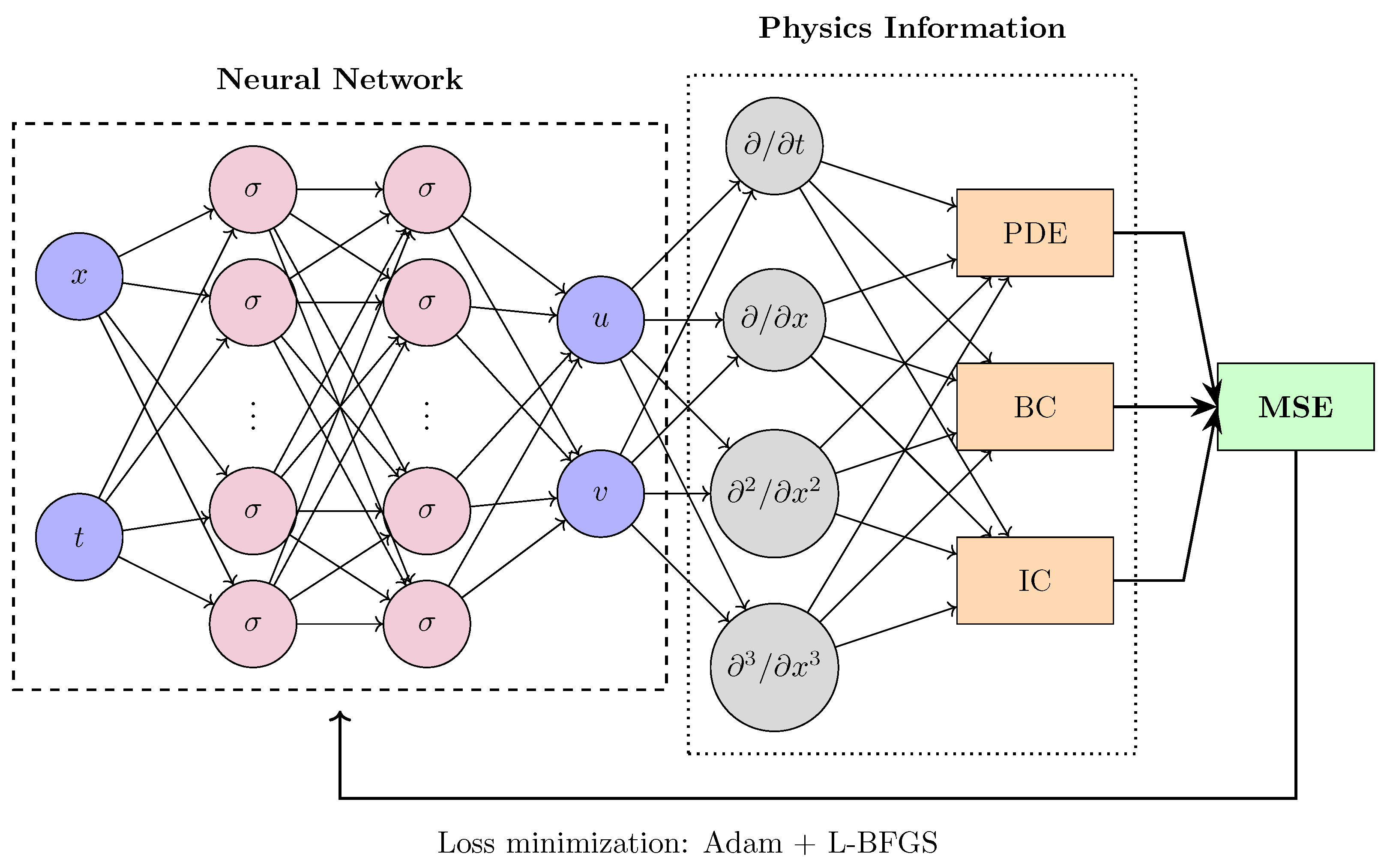
4. Physics-Informed Neural Network Technique

Physics-informed neural networks were first introduced in an initial preprint by Raissi, Perdikaris, and Karniadakis on arXiv in 2017 [13], followed by the formal publication in 2019 [14] along with the publicly available computer code [15]. Subsequently, an increasing number of publications have appeared dedicated to applications of this method in various scientific fields; for examples, see, the review articles [108,109] and references therein. In the following, we discuss the PINN framework in great detail.

4.1. Problem Statement

We describe the PINN method following [14]. Consider a parameterized nonlinear PDE of the following general form:

$${\displaystyle \frac{\partial q}{\partial t}}+\mathcal{N}[q,q_x,q_{xx},q_{xxx},\dots ]=0,x\in \mathbb{R},t\in [0,T]$$

(17)

where $q(x,t)=u(x,t)+iv(x,t)$ is the complex-valued solution, and $\mathcal{N}[q,q_x,q_{xx},q_{xxx},\dots ]$ is a nonlinear functional of the solution $q(x,t)$ and its derivatives of arbitrary orders with respect to x.

A PINN with the schematic shown in Figure 1 approximates both the solution $q(x,t)$ and the differential equation residual $f:={\displaystyle \frac{\partial q}{\partial t}}+\mathcal{N}[q,q_x,q_{xx},q_{xxx},\dots ]$ using a deep neural network [110,111,112,113]. The residual is decomposed into its real and imaginary parts as $f=f_u+i{f}_v$ and is computed via automatic differentiation [114], which applies the chain rule to the network outputs. The shared parameters between the networks for $q(x,t)$ and $f(x,t)$ are optimized by minimizing the total mean squared error (MSE) loss:

$$MSE=MS{E}_0+MS{E}_b+MS{E}_f$$

(18)

where the individual loss terms are defined as follows

$$\begin{array}{cc}\hfill MS{E}_0& ={\displaystyle \frac{1}{N_0}}\sum _{j=1}^{N_0}\left({\left|u(x_0^j,0)-u_0^j\right|}^2+{\left|v(x_0^j,0)-v_0^j\right|}^2\right),\hfill \end{array}$$

(19)

$$\begin{array}{cc}\hfill MS{E}_b& ={\displaystyle \frac{1}{N_b}}\sum _{j=1}^{N_b}\left({\left|u(-L,t_b^j)-u(L,t_b^j)\right|}^2+{\left|v(-L,t_b^j)-v(L,t_b^j)\right|}^2\right),\hfill \end{array}$$

(20)

$$\begin{array}{cc}\hfill MS{E}_f& ={\displaystyle \frac{1}{N_f}}\sum _{j=1}^{N_f}\left({\left|f_u(x_f^j,t_f^j)\right|}^2+{\left|f_v(x_f^j,t_f^j)\right|}^2\right).\hfill \end{array}$$

(21)

Here, ${(x_0^j,q_0^j)}_{j=1}^{N_0}$ with $q_0^j=u_0^j+i{v}_0^j$ denotes the initial training data sampled at $N_0$ discrete spatial points at $t=0$, ${\left(t_b^j\right)}_{j=1}^{N_b}$ represents $N_b$ collocation times used to enforce periodic boundary conditions at the spatial boundaries $x=\pm L$, and ${(x_f^j,t_f^j)}_{j=1}^{N_f}$ are $N_f$ collocation points used to evaluate the PDE residual $f(x,t)$ within the spatial–temporal domain $(x,t)\in (-L,L)\times (t_0,T]$.

The sampling points are usually generated using sampling strategies, i.e., the space-filling latin hypercube sampling (LHS) [115,116]. The loss function is minimized using gradient-based optimization algorithms. In practice, both the Adam [117] optimizer (a first-order method designed for stochastic objectives) and the limited memory Broyden–Fletcher–Goldfarb–Shannon (L-BFGS) [118] (a quasi-Newton, full-batch optimizer) are employed in sequence or combination to learn the optimal parameters. The implementation is based on TensorFlow [119], which is the most popular and well-documented open-source software library for automatic differentiation and deep learning computations.

The authors of the PINNs framework [14] noted that “Despite the fact that there is no theoretical guarantee that this procedure converges to a global minimum, our empirical evidence indicates that, if the given partial differential equation is well-posed and its solution is unique, our method is capable of achieving good prediction accuracy given a sufficiently expressive neural network architecture and a sufficient number of collocation points $N_f$”. In order to validate the accuracy of predictions made by PINNs, the relative ${\mathbb{L}}_2$ error between the predicted solution $\widehat{q}(x,t)$ and the exact solution $q(x,t)$ is usually computed:

$$\mathrm{Relative}{\mathbb{L}}_2\mathrm{error}={\displaystyle \frac{\sqrt{{\displaystyle \sum _{j=1}^N{\left|\widehat{q}(x_j,t_j)-q(x_j,t_j)\right|}^2}}}{\sqrt{{\displaystyle \sum _{j=1}^N{\left|q(x_j,t_j)\right|}^2}}}}$$

(22)

where $(x_j,t_j)$ are the collocation points in the spatial–temporal domain.

4.2. Examples of NLSE Solutions Computed with PINNs

To illustrate the PINN algorithm, we begin by solving the standard NLSE, which corresponds to Equation (7) in the special case where the coefficients $D_2=R_2=1$ and where $D_3$, $R_3$, $D_4$, $R_4$, $D_5$, $R_5$, and ${\lambda }_1$ are set to zero. The NLSE solutions are computed using the PINN approach and subject to periodic boundary conditions following Ref. [14]:

$$\left\{\begin{array}{cc}\hfill i{q}_t+{\displaystyle \frac{1}{2}}{q}_{xx}+{\left|q\right|}^{2}q& =0,x\in [-5,5],t\in \left[0,{\displaystyle \frac{\pi }{2}}\right],\hfill \\ \hfill q(0,x)& =2\mathrm{sech}\left(x\right),\hfill \\ \hfill q(t,-5)& =q(t,5),q_x(t,-5)=q_x(t,5)\hfill \end{array}\right.$$

(23)

where $q(x,t)$ is the complex-valued solution.

Figure 2 depicts the implementation of the PINN technique for solving the problem provided in Equation (23). The exact two-soliton bound-state solution, shown in Figure 2a, is formed by solitons with initial amplitudes ${\eta }_1=1.5$, ${\eta }_2=0.5$ and zero initial velocities ${\kappa }_1={\kappa }_2=0$, and was first obtained by Satsuma and Yajima in 1974 [120]. It is characterized by periodic oscillations with a period of $\pi /2$, and its initial shape $q(0,x)=2\mathrm{sech}\left(x\right)$ is periodically reproduced. Figure 2b shows a comparison between the numerically predicted solution $\left|q\right(x,t\left)\right|$ from the PINN model with the exact solution at multiple times, while Figure 2c shows the absolute error heatmap for $\left|q\right(x,t\left)\right|$ over the full spatial–temporal domain.

All simulations in this study and in the following were carried out using Python 3.8 and TensorFlow 2.12 on a machine equipped with an NVIDIA GeForce GTX 1080 graphics card (sourced: NVIDIA Corporation, Santa Clara, CA, USA). The PINN architecture consists of three hidden layers with 40 neurons each trained using 100 initial condition points ($N_0$), 200 boundary condition points ($N_b$), and 20,000 collocation points ($N_f$), with the LHS method used for selection to enforce the residual of Equation (23). To handle the complex solution $q(x,t)$, the network’s outputs are split into real and imaginary parts and derivatives are computed via automatic differentiation on each component. The training is performed in two stages. First, we use 10,000 iterations of the Adam optimizer with a learning rate of ${10}^{-3}$. The optimizer parameters are set to ${\beta }_1=0.9$ and ${\beta }_2=0.999$, which control the exponential decay rates for the first and second moment estimates, respectively. To further improve accuracy, we then switch to the L-BFGS optimizer, configured with a maximum of 10,000 steps, maxcor = 50, maxls = 50, and a convergence tolerance of ${10}^{-16}$, allowing for high-precision refinement of the solution. With this configuration, the relative ${\mathbb{L}}_2$ error is found to be $4.78\times {10}^{-3}$, demonstrating that the PINN can accurately capture the nonlinear soliton dynamics of the NLSE using only a small set of training data.

Figure 3a shows an example of the elastic interaction of two NLSE solitons with initial parameters ${\eta }_1=0.5$, ${\kappa }_1=-1.0$, and ${\eta }_2=0.5$, ${\kappa }_2=1.0$. We compare the exact solution with the predicted solution obtained from the PINN simulation in Figure 3b and show the absolute error in Figure 3c. The NN architecture consists of four hidden layers with 80 neurons each, using $N_0=100$, $N_b=200$, and $N_f=20,000$. The network was trained with 20,000 iterations of the Adam optimizer followed by 20,000 steps of L-BFGS on a spatial–temporal domain bounded by $x\in [0,20]$ and $t\in [0,5]$. The resulting relative ${\mathbb{L}}_2$ error for $\left|q\right(x,t\left)\right|$ is found to be $8.52\times {10}^{-3}$.

Following the innovative work of [14], various solitary wave solutions of the standard and modified NLSE have been investigated using PINN-based approaches, including solitons, breathers, rogue waves, and peakons [20,21,24,31,36,37,39,43,53]. These results have consistently proved that physics-informed deep learning methods can accurately reproduce the dynamical behavior of such nonlinear wave structures.

However, there are several challenges when applying PINNs, particularly in accurately capturing the time dynamics of nonlinear systems. These problems often limit the time intervals over which solutions can be reliably learned [121]. Similar difficulties are particularly pronounced for breathers and other periodic solutions, which require not only a broader temporal domain but also modifications to the loss function or domain decomposition [16,26].

One proposed strategy for improving the learning performance of PINNs is to include additional physical constraints such as energy and momentum conservation laws directly in the loss function [24]. This approach can help to guide the network towards physically meaningful solutions and leads to more accurate prediction of soliton and breather dynamics [122].

In addition, various forms of regularization have been introduced to improve generalization and prevent overfitting, especially when only limited training data are available [123,124]. Another direction of improvement is related to the optimization of the learning rate, as neural network training can easily fall into local minima [18,24,26,27]. It has been shown that using a variable learning rate in which the initial value is gradually reduced during training can lead to smoother loss curves, faster convergence, and better overall accuracy. The current state of PINN technologies along with their respective advantages and challenges have been discussed in a number of recent reviews [108,109,125,126].

Several recent studies [127,128,129,130,131,132] have conducted direct comparisons between PINNs and classical numerical solvers (e.g., finite element, finite difference, or spectral methods) in terms of accuracy and computational cost. In particular, Ortiz et al. [131] presented a qualitative comparison between the classical Fourier-based Crank–Nicolson method [133] and the PINN framework for the generalized KdV equation. The authors showed that while the spectral Crank–Nicolson method offers superior accuracy and speed, PINNs provide greater flexibility for handling noisy data and multi-soliton dynamics, albeit at higher computational cost. In [132], PINNs were applied to solve the one-dimensional classical Reynolds equation. The main objective of the authors was to compare the solutions obtained using PINNs and the finite difference numerical method with the exact analytical solution. To construct an optimal neural network, the authors studied various scenarios with diverse hyperparameters, including the learning rate, number of training points, etc. They concluded that while the finite difference method shows greater accuracy, PINNs are capable of solving problems where traditional discretization schemes are difficult to apply or where incorporation of problem-specific data is necessary. Therefore, the full potential of PINNs remains to be determined. Most studies [127,128,130,131,132] have shown that PINNs are best considered as a complement to traditional numerical methods rather than as a complete replacement. A general conclusion is that optimal strategies can involve choosing the most suitable solver for a given class of PDEs as well as a symbiosis of these two approaches [108,109,125,126,127,128,129,130,131,132].

4.3. Application of PINNs for the NLSE with External Potentials

One promising application of physics-informed deep learning methods is the study of solitary wave dynamics under external potentials. A number of studies have demonstrated that PINNs can accurately reproduce such solutions [30,31,37,39].

In [31], the NLSE with the generalized $\mathcal{PT}$-symmetric Scarf-II potential was analyzed based on the PINN technique. The authors applied the Dirichlet boundary condition along with three others to calculate optical solitons, instability solutions, and a hyperbolic secant function with one constant. The effects of optimization steps and activation functions on the performance of the PINNs were investigated. The obtained results were then compared with those derived by the traditional numerical methods. The results showed that the PINN method can effectively learn the NLSE with the generalized $\mathcal{PT}$-symmetric Scarf-II potential.

The authors of [39] analyzed soliton solutions of the NLSE with three $\mathcal{PT}$-symmetric potentials: Gaussian, periodic, and Rosen–Morse. The training dataset consisted of 50 points for the initial condition, 100 points for the periodic boundary conditions, and 20,000 randomly selected collocation points obtained using the LHS algorithm. The PINN architecture consisted of four hidden layers with 100 neurons each, while the spatial and temporal domains were set as $x\in [-10,10]$ and $t\in [0,5]$. The network was trained over 40,000 steps using the L-BFGS algorithm and approximated the soliton solutions of the NLSE with all three potentials, achieving ${\mathbb{L}}_2$ errors of $3.2\times {10}^{-3}$, $4.2\times {10}^{-3}$, and $5.0\times {10}^{-3}$ for the Gaussian, periodic, and Rosen–Morse potentials, respectively.

As an illustration, we solve the NLSE with a linear potential and analyze its soliton solutions using the PINN approach:

$$i{q}_t+{\displaystyle \frac{1}{2}}{D}_2{q}_{xx}+R_2{\left|q\right|}^{2}q-2{\lambda }_{1}xq=0.$$

(24)

For this case, Equations (15) and (16) take the following form:

$$\begin{array}{cc}\hfill \xi (x,t)& =2\left(x-x_0\right){\eta }_0+2D_2{\eta }_0\left(2{\kappa }_{0}t+{\lambda }_1{t}^2\right),\hfill \\ \hfill \chi (x,t)& =2\left(x-x_0\right)\left({\kappa }_0+{\lambda }_{1}t\right)+2D_2\left[\left({\kappa }_0^2-{\eta }_0^2\right)t+{\lambda }_1{t}^2+{\displaystyle \frac{{\lambda }_1^2}{3}}{t}^3\right],\hfill \end{array}$$

(25)

with constant soliton amplitude $\eta ={\eta }_0$ and time-varying velocity $\kappa \left(t\right)={\kappa }_0+{\lambda }_{1}t$, where ${\eta }_0$ and ${\kappa }_0$ correspond to the initial amplitude and velocity of the soliton, respectively.

The implementation procedure for solving Equation (24) follows the same steps outlined earlier. The unknown solution $q(x,t)$ is separated into its real part $u(x,t)$ and imaginary part $v(x,t)$, resulting in the complex-valued multi-output PINN shown below.

def f_uv(x, t):

   u, v = q(x, t)

   u_x = tf.gradients(u, x)[0]

   v_x = tf.gradients(v, x)[0]

   u_t = tf.gradients(u, t)[0]

   v_t = tf.gradients(v, t)[0]

   u_xx = tf.gradients(u_x, x)[0]

   v_xx = tf.gradients(v_x, x)[0]

   f_u = −v_t + 0.5∗D2∗u_xx + R2∗(u∗∗2 + v∗∗2)∗u − 2 ∗ lambda ∗ x ∗ u

   f_v =  u_t + 0.5∗D2∗v_xx + R2∗(u∗∗2 + v∗∗2)∗v − 2 ∗ lambda ∗ x ∗ v

   return f_u, f_v

Figure 4 shows the results of the simulations. The exact one-soliton solution of Equation (24) calculated with amplitude $\eta =1$, initial velocity ${\kappa }_0=1.75$, and ${\lambda }_1=-3.5$ is shown in Figure 4a. The dispersion and nonlinearity coefficients are set to $D_2=R_2=1.0$, and the initial solution at $t=0$ is written as follows: $q(x,t)=2{\eta }_0\mathrm{sech}\left(2{\eta }_{0}x\right)exp(-2i{\kappa }_{0}x)$. We compare the exact solution with the predicted solution obtained from the PINN simulation in Figure 4b and show the absolute error in Figure 4c. The network architecture consists of four hidden layers with 40 neurons each, using $N_0=50$, $N_b=100$, and $N_f=20,000$ with the LHS sampling. The network was trained with 20,000 iterations of the Adam optimizer followed by 20,000 steps of L-BFGS on a spatial–temporal domain bounded by $x\in [-5,5]$ and $t\in [0,1]$. The resulting relative ${\mathbb{L}}_2$ errors are $3.51\times {10}^{-3}$ for u, $2.42\times {10}^{-3}$ for v, and $2.04\times {10}^{-3}$ for $\left|q\right(x,t\left)\right|$. Hence, we conclude that this physics-informed deep learning approach is a powerful algorithm able to solve the NLSE with various external potentials.

4.4. Performance Analysis of the PINN Method

In order to evaluate the predictive capacity of the PINN methodology, we analyze some of its key elements, following Refs. [13,14,17]. These elements include the effects of different activation functions, network architectures, numbers of sampling points, and sampling strategies used for training. A series of numerical tests based on the one-soliton solution of the NLSE with a linear potential provided in Equation (24) was carried out on a spatial–temporal domain bounded by $x\in [-5,5]$ and $t\in [0,1]$.

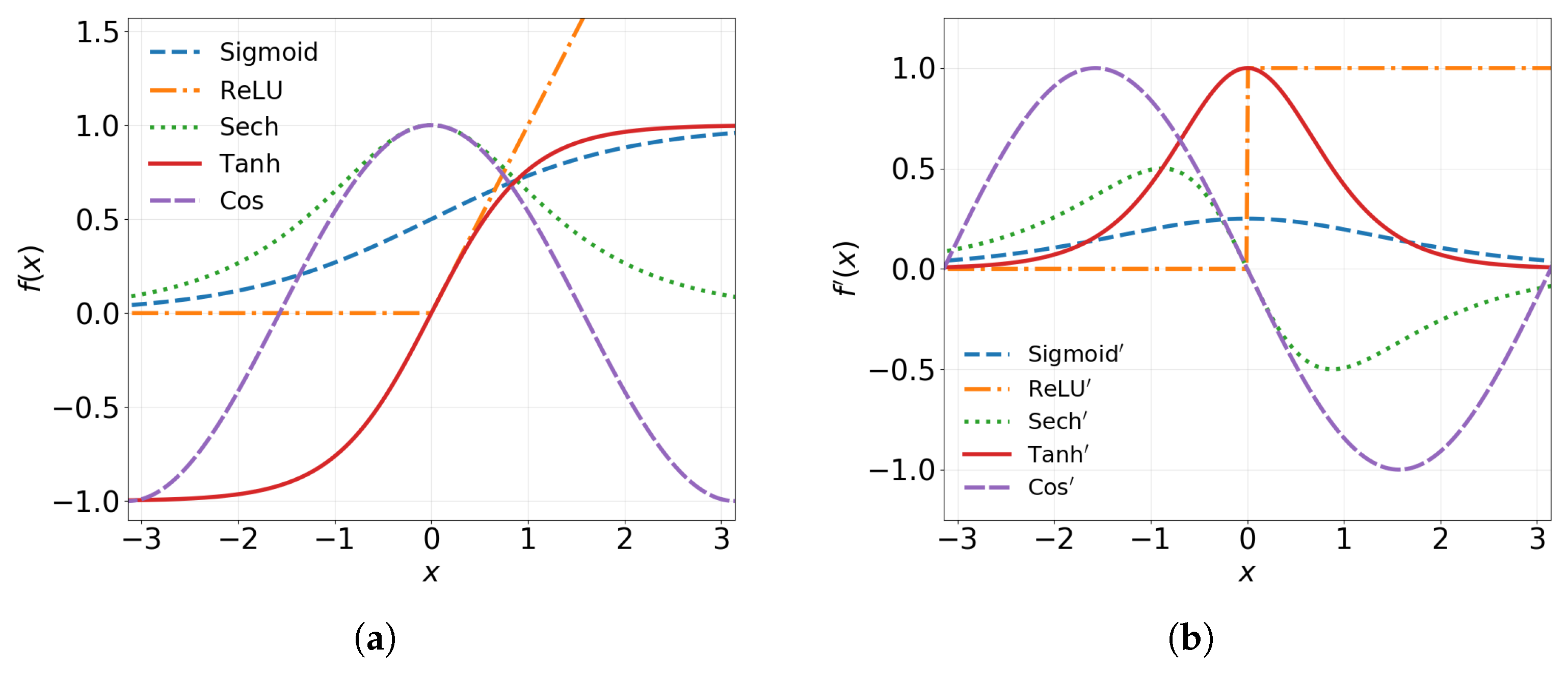
4.4.1. Impact of the Activation Functions

In order to introduce nonlinearity and enable learning of complex patterns, an activation function is applied to the output of each neuron. The weights in the NN are updated iteratively using gradient descent, where the update rule depends on the gradient of a scalar-valued loss function $\mathcal{L}$ with respect to the weights at each layer. The update rule for the weights w in layer k is provided by

$$w^{\left(k\right)}:=w^{\left(k\right)}-\eta {\displaystyle \frac{\partial \mathcal{L}}{\partial w^{\left(k\right)}}},$$

(26)

where $\eta$ is the learning rate and ${\displaystyle \frac{\partial \mathcal{L}}{\partial w^{\left(k\right)}}}$ is the gradient of the loss with respect to the weights. As an example, for a fully connected feedforward network with three hidden layers, the gradients with respect to the weights in the last three layers can be expanded as follows:

$$\begin{array}{cc}\hfill {\displaystyle \frac{\partial \mathcal{L}}{\partial w^{\left(3\right)}}}& ={\displaystyle \frac{\partial \mathcal{L}}{\partial \widehat{y}}}·{\displaystyle \frac{\partial \widehat{y}}{\partial w^{\left(3\right)}}},\hfill \\ \hfill {\displaystyle \frac{\partial \mathcal{L}}{\partial w^{\left(2\right)}}}& ={\displaystyle \frac{\partial \mathcal{L}}{\partial \widehat{y}}}·{\displaystyle \frac{\partial \widehat{y}}{\partial a^{\left(3\right)}}}·{\displaystyle \frac{\partial a^{\left(3\right)}}{\partial z^{\left(3\right)}}}·{\displaystyle \frac{\partial z^{\left(3\right)}}{\partial w^{\left(2\right)}}},\hfill \\ \hfill {\displaystyle \frac{\partial \mathcal{L}}{\partial w^{\left(1\right)}}}& ={\displaystyle \frac{\partial \mathcal{L}}{\partial \widehat{y}}}·{\displaystyle \frac{\partial \widehat{y}}{\partial a^{\left(3\right)}}}·{\displaystyle \frac{\partial a^{\left(3\right)}}{\partial z^{\left(3\right)}}}·{\displaystyle \frac{\partial z^{\left(3\right)}}{\partial a^{\left(2\right)}}}·{\displaystyle \frac{\partial a^{\left(2\right)}}{\partial z^{\left(2\right)}}}·{\displaystyle \frac{\partial z^{\left(2\right)}}{\partial w^{\left(1\right)}}},\hfill \end{array}$$

(27)

where $\widehat{y}$ denotes the network output, $z^{\left(k\right)}$ is the pre-activation value obtained from the linear transformation in layer k, and $a^{\left(k\right)}=\sigma \left(z^{\left(k\right)}\right)$ is the activated output, where $\sigma$ represents the activation function.

Various activation functions have been proposed, including several trigonometric and hyperbolic functions along with the well-known sigmoid [4] and rectified linear unit (ReLU) [6] functions, for which the explicit functional forms are provided in

Table 1. Common nonlinear activation functions along with their expressions and derivatives. The relative ${\mathbb{L}}_2$ error between the predicted and exact solution $q(x,t)$ is shown for different activation functions.

Function	Expression	Derivative	Relative ${\mathbb{L}}_2$ Error
Sigmoid	${\displaystyle \sigma \left(x\right)=\frac{1}{1+e^{-x}}}$	${\displaystyle \sigma \left(x\right)(1-\sigma (x\left)\right)}$	$1.23\times {10}^{-1}$
ReLU	${\displaystyle max(0,x)}$	${\displaystyle \left\{\begin{array}{cc}0\hfill & x<0\hfill \\ 1\hfill & x>0\hfill \end{array}\right.}$	$8.71\times {10}^{-1}$
Sech	${\displaystyle \mathrm{sech}\left(x\right)=\frac{2}{e^x+e^{-x}}}$	${\displaystyle -\mathrm{sech}\left(x\right)tanh\left(x\right)}$	$1.00\times {10}^{-2}$
Tanh	${\displaystyle tanh\left(x\right)=\frac{e^x-e^{-x}}{e^x+e^{-x}}}$	${\displaystyle 1-{tanh}^2\left(x\right)}$	$2.04\times {10}^{-3}$
Cos	${\displaystyle cos\left(x\right)}$	${\displaystyle -sin\left(x\right)}$	$1.18\times {10}^{-3}$

. A comparison of the most common activation functions and their derivatives is shown in Figure 5. The activation functions must be smooth in order to avoid vanishing gradients during backpropagation [4]. This is an essential requirement during the training of a PINN, as the loss function incorporates higher-order derivatives.

In the following, we perform a study to assess the impact of the activation function on the performance of a PINN while solving Equation (24). The PINN consists of four hidden layers with 40 neurons each, and the network is trained with 20,000 iterations of the Adam optimizer followed by 20,000 steps of L-BFGS. The number of initial and boundary training data points is fixed at $N_u=150$, while the number of collocation points is $N_f=20,000$, selected using the LHS method. Table 1 reports the relative ${\mathbb{L}}_2$ errors in approximating the exact solution of Equation (24) using different nonlinear activation functions. The cosine activation function yields the lowest relative error, followed by $tanh\left(x\right)$ and $\mathrm{sech}\left(x\right)$. On the other hand, the slow convergence of the sigmoid function and the lack of smoothness in the ReLU function lead to significantly poorer performance. Our results confirm that smooth and differentiable activation functions are more suitable in the context of physics-based learning [134,135].

4.4.2. Impact of Neural Network Architecture

The parameters of a neural network have a significant influence on its predictive accuracy and convergence. Among the different parameters, depth (number of hidden layers) and width (number of neurons per layer) are especially important when designing PINN architectures. In the following, we examine the effect of these choices on the performance of the method in solving Equation (24).

Table 2. Relative ${\mathbb{L}}_2$ error estimations between the predicted and exact solution $q(x,t)$ of Equation (24) for different numbers of network layers and neurons per hidden layer.

Neurons	Hidden Layers
	2	4	6	8
10	$1.31\times {10}^{-1}$	$6.59\times {10}^{-2}$	$7.51\times {10}^{-2}$	$5.26\times {10}^{-2}$
20	$1.09\times {10}^{-1}$	$1.43\times {10}^{-2}$	$1.38\times {10}^{-2}$	$1.51\times {10}^{-2}$
40	$6.10\times {10}^{-2}$	$2.04\times {10}^{-3}$	$1.86\times {10}^{-3}$	$1.45\times {10}^{-3}$
60	$9.01\times {10}^{-2}$	$1.51\times {10}^{-3}$	$1.23\times {10}^{-3}$	$1.03\times {10}^{-3}$
80	$5.51\times {10}^{-2}$	$2.52\times {10}^{-3}$	$1.16\times {10}^{-3}$	$1.33\times {10}^{-3}$

reports the relative ${\mathbb{L}}_2$ errors for various configurations of hidden layers and neurons per hidden layer. All models are trained with a fixed number of initial and boundary points ($N_u=150$) and collocation points ($N_f=20,000$) using LHS in the same spatial–temporal domain. The number of training iterations is kept constant, with 20,000 steps using the Adam optimizer followed by an additional 20,000 steps of L-BFGS optimization.

We observe that increasing the network capacity improves the accuracy of numerical prediction, whether adding more neurons or increasing the number of layers. In particular, the configuration with 60 neurons and 8 hidden layers achieves the best accuracy, with a ${\mathbb{L}}_2$ error of $1.03\times {10}^{-3}$ between the predicted and exact solution of $q(x,t)$. We also observe that although increasing the network width beyond 40 neurons continues to reduce the error, the improvement eventually becomes marginal, suggesting a saturation point in terms of model capacity.

4.4.3. Impact of the Number of Sampling Points

To further analyze the performance of the PINN method, we performed a study to quantify its predictive accuracy in solving Equation (24) for different number of initial and boundary training points $N_u$ and collocation points $N_f$.

Table 3. Relative ${\mathbb{L}}_2$ error estimations between the predicted and exact solution $q(x,t)$ of Equation (24) for different numbers of initial and boundary training points $N_u$ and collocation points $N_f$.

Initial/Boundary Points, ${\mathit{N}}_{\mathit{u}}$	Collocation Points, ${\mathit{N}}_{\mathit{f}}$
	5000	10,000	15,000	20,000
60	$8.62\times {10}^{-1}$	$1.54\times {10}^{-2}$	$1.62\times {10}^{-2}$	$1.29\times {10}^{-2}$
90	$1.06\times {10}^{-2}$	$3.14\times {10}^{-3}$	$3.37\times {10}^{-3}$	$3.84\times {10}^{-3}$
120	$8.74\times {10}^{-3}$	$3.37\times {10}^{-3}$	$4.59\times {10}^{-3}$	$4.28\times {10}^{-3}$
150	$6.53\times {10}^{-3}$	$1.90\times {10}^{-3}$	$2.20\times {10}^{-3}$	$2.04\times {10}^{-3}$
180	$7.78\times {10}^{-3}$	$1.97\times {10}^{-3}$	$2.85\times {10}^{-3}$	$3.23\times {10}^{-3}$
240	$6.20\times {10}^{-3}$	$2.68\times {10}^{-3}$	$1.53\times {10}^{-3}$	$2.64\times {10}^{-3}$
300	$4.71\times {10}^{-3}$	$3.25\times {10}^{-3}$	$2.50\times {10}^{-3}$	$2.56\times {10}^{-3}$

shows the relative ${\mathbb{L}}_2$ errors between the predicted and exact solution of $q(x,t)$ obtained for different combinations of $N_u$ and $N_f$ using a fixed four-layer network architecture with 40 neurons per hidden layer. The values of $N_u$ refer to the total number of randomly sampled training points, and are composed of both the initial data at $t=0$ and the boundary data along the spatial domain. The number of training iterations is kept constant, with 20,000 steps of Adam and 20,000 steps of L-BFGS minimization.

In general, the results indicate that increasing $N_u$ leads to improved accuracy, provided that a sufficient number of collocation points is used; for example, with only 60 data points, the model performs poorly when $N_f$ is small (e.g., $8.62\times {10}^{-1}$ for $N_f=5000$), but improves when $N_f$ increases. Our results reinforces a key advantage of the PINN framework: by incorporating physical constraints through the residual loss at collocation points, the model requires fewer labeled data points to achieve high accuracy. In our case, increasing $N_u$ beyond 150 points does not lead to a significant improvement in accuracy. The lowest ${\mathbb{L}}_2$ error is achieved at $N_u=240$ and $N_f=15,000$, suggesting that moderately sized training sets are already effective for this particular study when combined with sufficient collocation points.

4.4.4. Impact of the Sampling Method

The choice of sampling method can significantly influence the accuracy and efficiency of a PINN’s numerical solution [51,52,136,137,138,139]. In the following, we study the impact of different sampling techniques for placement of the collocation points and their influence on the relative ${\mathbb{L}}_2$ error, which is applied to the NLSE with linear potential provided in Equation (24).

In particular, we consider two uniform sampling methods: deterministic equidistance uniform grid, and random sampling from a continuous uniform distribution over the computational domain. In addition to these basic approaches, we explore two quasi-random sequences: the LHS [115,116] and the Sobol sequence [140]. Figure 6 presents an illustration of these four sampling techniques, which are applied to 900 points sampled in the domain $[0,1]\times [0,1]$.

We performed a test to quantify the numerical precision of PINNs in solving Equation (24) using a fixed network architecture consisting of four hidden layers with 40 neurons each. Training is performed using 20,000 iterations of the Adam optimizer followed by 20,000 steps of L-BFGS, and the number of initial and boundary data points is fixed at $N_u=150$.

The results are summarized in

Table 4. Relative ${\mathbb{L}}_2$ error estimations between the predicted and exact solution $q(x,t)$ of Equation (24) for different sampling methods.

Sampling Method	Collocation Points, ${\mathit{N}}_{\mathit{f}}$
	5000	20,000
Grid	$5.02\times {10}^{-3}$	$3.16\times {10}^{-3}$
Random	$6.03\times {10}^{-3}$	$2.39\times {10}^{-3}$
LHS	$6.53\times {10}^{-3}$	$2.04\times {10}^{-3}$
Sobol	$4.36\times {10}^{-3}$	$1.77\times {10}^{-3}$

. Among all methods tested, the Sobol sequence consistently achieves the lowest relative ${\mathbb{L}}_2$ error, outperforming the LHS, random, and grid sampling methods. In the case of a reduced number of collocation points, $N_f=5000$, the grid and random sampling methods reach errors of $5.02\times {10}^{-3}$ and $6.03\times {10}^{-3}$, respectively, while LHS performs slightly worse at $6.53\times {10}^{-3}$. In the case of $N_f=20,000$, the LHS sampling strategy shows better accuracy compared to the grid and random sampling methods. Our observations confirm the efficient collocation point distribution achieved by the quasi-random Sobol sequence, which improves the accuracy of the PINN solution.

5. Examples of Higher-Order NLSE Hierarchy Solutions Computed with PINNs

To further illustrate the application of PINNs, in this section we review several examples of their application to numerically solving the third-, fourth-, and fifth-order equations of the NLSE hierarchy.

5.1. PINN Application to the Complex mKdV Equation

The complex modified Korteweg–de Vries (cmKdV) equation

$$i{q}_t+i{D}_3{q}_{xxx}+6i{R}_3{\left|q\right|}^2{q}_x=0$$

(28)

is the first equation of the third order of the NLSE hierarchy. Applications of PINNs for the cmKdV equation have been studied in [34,35].

The rational wave solutions and soliton molecules were numerically studied in [34] using a fully connected deep NN with eight hidden layers and 50 neurons per each hidden layer. The network was trained using the stochastic gradient descent calculation with the Adam optimizer. The authors concluded that the PINN approach often has difficulty in exactly approximating the solutions of this nonlinear differential equation, and proposed reducing gradient fluctuations by examining different loss functions or using more efficient neural network architectures, among other approaches.

In [35], the authors optimized the training process by modifying a loss function composed of initial conditions and boundary conditions. They tested the performance of their models comparing with traditional PINNs by calculating the high-order rogue waves of the cmKdV equation using NNs with up to 80 neurons in eight hidden layers. Their results obtained showed that while the original PINNs could not simulate second-order and third-order rogue waves of the cmKdV equation, their proposed changes significantly improved the simulation capability and improved prediction accuracy by orders of magnitude.

Recently, Wang et al. [41] studied the dynamics of data-driven solutions and identified the unknown parameters of the nonlinear dispersive modified KdV-type equation using PINNs. They simulated various soliton and anti-soliton solutions and their combinations as well as the kink, peakon, and periodic solutions. Their analysis showed that these PINNs could solve mKdV-type equations with relative ${\mathbb{L}}_2$ errors of $\mathcal{O}\left({10}^{-3}\right)$ or $\mathcal{O}\left({10}^{-4}\right)$ for the multi-soliton and kink solutions, respectively, while relative errors for the peakon and periodic solutions reached $\mathcal{O}\left({10}^{-2}\right)$. In addition, they analyzed several activation functions and concluded that the $\tanh \left(\mathbf{x}\right)$ function provided the best training performance.

We illustrate an application of PINNs to solve the complex mKdV equation in Figure 7, which shows the dynamics of the two-soliton bound state. Solitons with initial amplitudes ${\eta }_1=0.4$, ${\eta }_2=0.1$ and initial velocities ${\kappa }_1=1.5$, ${\kappa }_2=1.48$ are initially placed at the same starting point $x_1=x_2=1.0$ at $t=0$, forming an envelope breather solution filled with high-frequency oscillations that satisfies the condition ${\eta }_i/{\kappa }_i\ll 1$. The dispersion and nonlinearity coefficients are set to $D_3=R_3=0.1$. Figure 7a shows the dynamics of the bound state of two solitons of the cmKdV equation over the spatial–temporal domain bounded by $x\in [-10,10]$ and $t\in [0,1]$. We compare the exact solution with the predicted solution obtained from the PINN simulation in Figure 7b, and show the absolute error in Figure 7c. The PINN architecture consists of five hidden layers with 100 neurons each, using $N_0=100$, $N_b=200$, and $N_f=20,000$. The network is trained with 50,000 iterations of the Adam optimizer followed by 20,000 steps of L-BFGS. The resulting relative ${\mathbb{L}}_2$ error for $\left|q\right(x,t\left)\right|$ is found to be $3.34\times {10}^{-2}$.

5.2. PINN Application for the Hirota Equation

The numerical solutions of the Hirota equation [62]

$$i{q}_t+{\displaystyle \frac{1}{2}}{D}_2{q}_{xx}+R_2{\left|q\right|}^{2}q+i{D}_3{q}_{xxx}+6i{R}_3{\left|q\right|}^2{q}_x=0,$$

(29)

were studied using the PINN framework in Refs. [25,27,32,38,40].

In particular, the authors of [25] studied the one- and two-soliton solutions, rogue waves, and W- and M-soliton solutions of the Hirota equation using PINNs under different initial and periodic boundary conditions. Training was carried out using a neural network with up to 30 neurons in seven hidden layers, with 100 randomly sampled points from the initial and the periodic boundary data and 10,000 collocation points. The relative ${\mathbb{L}}_2$ error for the W- and M-soliton solutions was found to be around $9.13\times {10}^{-3}$ and $6.02\times {10}^{-3}$, respectively. However, it was observed that the error gradually increased as time progressed within the studied $t\in [0,5]$ interval. To address this, the authors optimized the NN structure by increasing the number of layers, neurons per layer, and sample points, which resulted in an overall increase in the computational time.

In [27], the authors proposed a feedforward NN consisting of two parallel sub-networks in order to numerically predict the nonlinear dynamics and formation processes of bright and dark picosecond optical solitons as well as femtosecond soliton molecules in single-mode fibers. Additional loss terms were introduced into the loss function, with the first subnet learning the real and imaginary parts of the solution and the second learning the first derivative of the solution. This architecture used five hidden layers with 40 neurons per layer, with adaptive weights introduced to accelerate convergence. Compared with standard PINNs, this approach improved the prediction accuracy by an order of magnitude.

We present the application of PINNs to solve the Hirota equation in Figure 8. We calculate the interaction of two solitons of Equation (29) with the initial soliton amplitudes ${\eta }_1=0.55$, ${\eta }_2=0.5$ and initial soliton velocities ${\kappa }_1=1.0$, ${\kappa }_2=-1.0$. The dispersion and nonlinearity coefficients are taken as follows: $D_2=R_2=1.0$ and $D_3=R_3=0.01$. Figure 8a shows the interaction of two solitons of the Hirota equation over the spatial–temporal domain bounded by $x\in [-10,10]$ and $t\in [0,4]$. We compare the exact solution with the predicted solution obtained from the PINN simulation in Figure 8b, and show the absolute error in Figure 8c. The PINN architecture consists of five hidden layers with 80 neurons each, using $N_0=50$, $N_b=100$, and $N_f=$ 20,000. The network is trained with 20,000 iterations of the Adam optimizer followed by 20,000 steps of L-BFGS. The resulting relative ${\mathbb{L}}_2$ error for $\left|q\right(x,t\left)\right|$ is found to be $5.47\times {10}^{-3}$.

5.3. PINN Application to Higher-Order Equations of the NLSE Hierarchy

The application of the PINN framework for solving higher-order integrable equations of the NLSE hierarchy has been investigated in [40]. There, the authors studied the evolution of positon solutions in the spatial and time range defined as $x,t\in [-10,10]$ using 100 initial condition points, 200 boundary condition points, and 10,000 collocation points. Their PINN architecture employed eight hidden layers with 40 neurons each, applying the hyperbolic tangent activation function and minimizing the loss function after 80,000 iterations via Adam optimization. The authors concluded that their algorithm is able to predict positon solutions not only in the standard NLSE but also in other higher-order versions, including cubic, quartic, quintic, and sextic equations of the NLSE hierarchy. It was shown that the PINN approach can also effectively handle two coupled NLSE equations and two coupled Hirota equations.

In order to further illustrate the capabilities of the PINN method, we provide examples of numerical calculations for the solutions of the fourth and fifth orders of the NLSE hierarchy provided in Equation (7) in the absence of a linear potential.

Figure 9 presents the application of PINNs to solve the truncated version of the fourth-order equation (known as the Lakshmanan–Porsezian–Daniel equation [85]) with the dispersion and nonlinearity coefficients $D_2=R_2=1.0$, $D_3=R_3=0.0$, and $D_4=R_4=1/64$. The interaction of two solitons of the fourth-order equation of the NLSE hierarchy over the spatial–temporal domain bounded by $x\in [-10,10]$ and $t\in [0,3]$ with the initial amplitudes ${\eta }_1=0.5$, ${\eta }_2=0.5$ and initial velocities ${\kappa }_1=1.0$, ${\kappa }_2=-1.0$ is shown in Figure 9a. We compare the exact solution with the predicted solution obtained from the PINN simulation in Figure 9b, and show the absolute error in Figure 9c. The NN architecture consists of five hidden layers with 80 neurons each, using $N_0=50$, $N_b=100$, and $N_f=$ 20,000 selected using the LHS method. The network achieves a relative ${\mathbb{L}}_2$ error of $8.25\times {10}^{-3}$ for $\left|q\right(x,t\left)\right|$, demonstrating that PINNs can accurately capture the fourth-order nonlinear soliton dynamics.

The interaction of two solitons of the fifth order of Equation (7) with the dispersion and nonlinearity coefficients set to $D_2=R_2=1.0$, $D_3=R_3=1/8$, $D_4=R_4=0.0$, and $D_5=R_5=1/32$ over the spatial–temporal domain bounded by $x\in [-10,10]$ and $t\in [0,2.5]$ is shown in Figure 10. The calculations correspond to the elastic interaction of two solitons with the initial amplitudes ${\eta }_1={\eta }_2=0.5$ and initial velocities ${\kappa }_1=1.0$, ${\kappa }_2=-1.0$.

Figure 10b shows the comparison between the numerically predicted solution $\left|q\right(x,t\left)\right|$ from the PINN model and the exact solution at multiple times, while Figure 10c shows the absolute error heatmap for $\left|q\right(x,t\left)\right|$ over the full spatial–temporal domain. The NN architecture consists of five hidden layers with 50 neurons each, using $N_0=50$, $N_b=50$, and $N_f=10,000$ selected using the LHS method. The network achieves a relative ${\mathbb{L}}_2$ error of $7.67\times {10}^{-2}$ for $\left|q\right(x,t\left)\right|$.

We observe that the PINN model struggles to capture the soliton dynamics; in particular, slight deviations between the predicted and exact solutions become more pronounced during the soliton interaction phase. This example demonstrates a limitation of the PINN approach when applied to more complex systems. In particular, the observed reduction in accuracy from the fourth-order case to the fifth-order one arises from the increased complexity of the governing equation as well as from the dynamics associated with two-soliton interaction. In order to address this deviation from the exact solution, it could be possible to increase the density of collocation points or employ a deeper network architecture, as demonstrated in Table 2 and Table 3. A thorough investigation of this specific configuration is beyond the scope of the present review, and will be addressed in an intended dedicated research study.

6. Conclusions and Perspectives

The results and methodologies discussed in this review highlight the synergy between modern machine learning techniques and analytical soliton theory, revealing a pathway toward solving higher-order nonlinear Schrödinger-type equations. We have summarized the application of physics-informed neural networks for solving the PDEs belonging to the nonlinear Schrödinger equation hierarchy, which arise not only in mathematical physics but also in diverse domains such as nonlinear optics, Bose–Einstein condensates, plasma dynamics, and quantum field theory.

We examine the literature on PINNs, beginning with the first papers from Raissi et al. [13,14] and continuing with the research on solving higher-order PDEs of the NLSE type, including models with external potentials. Our findings are summarized in

Table 5. Summary of PINN architectures employed for obtaining the numerical solution of nonlinear partial differential equations from the nonlinear Schrödinger equation hierarchy.

PDE and Type of Solution	Layers × Neurons	${\mathit{N}}_{\mathit{u}}$	Rel. ${\mathbb{L}}_2$ Error
NLS; Equation (23), 2-sol. bound state	$3\times 40$	300	$4.78\times {10}^{-3}$
NLS; Equation (23), 2-sol. interaction	$4\times 80$	300	$8.52\times {10}^{-3}$
NLS + linear potential; Equation (24), 1-sol.	$4\times 40$	150	$2.04\times {10}^{-3}$
cmKdV; Equation (28), 2-sol. bound state	$5\times 100$	300	$3.34\times {10}^{-2}$
Hirota; Equation (29), 2-sol. interaction	$5\times 80$	150	$5.47\times {10}^{-3}$
Fourth-order NLS; Equation (7), 2-sol. interaction	$5\times 80$	150	$5.47\times {10}^{-3}$
Fifth-order NLS; Equation (7), 2-sol. interaction	$5\times 50$	150	$7.67\times {10}^{-2}$

, where we compare the achieved relative ${\mathbb{L}}_2$ errors between the predicted and exact soliton solutions of the different equations studied in this review. The soliton solutions are indicated as one-soliton (1-sol.) or two-soliton (2-sol.) interaction or bound-state. The number of hidden layers and neurons per layer along with the total number of initial and boundary points ($N_u$) selected using the LHS method are shown for each PDE. All networks use the $tanh\left(x\right)$ activation function, with the number of collocation points fixed at $N_f=20,000$ except for the fifth-order case, where $N_f=10,000$. Training was performed using 20,000 iterations of the Adam optimizer followed by 20,000 steps of L-BFGS for all cases except for the two-soliton bound-state example of the NLS, where 10,000 iterations were used for both optimizers.

Our analysis of the contemporary literature confirms that PINNs are a valuable tool in the study of nonlinear evolution equations and offer new opportunities for both analytical and computational exploration. Nevertheless, several challenges remain [19,121]. Learning long-time dynamics is difficult, especially for breathers and other periodic solutions, which require a larger temporal domain and adjustments to the loss function or domain decomposition [16,26]. To improve learning performance, the inclusion of additional physical constraints such as energy and momentum conservation laws directly into the loss function has been successfully applied [24,122]. Regularization techniques have also been introduced to prevent overfitting, especially when limited training data are available [123,124]. Recent studies have proposed various strategies to mitigate the challenges associated with long-time integration in PINNs, adopting sequential learning or time-marching strategies [141,142,143]. This limitation has also been attributed to the inability of existing PINN formulations to respect the spatial–temporal causal structure when solving PDEs [144], and continues to be an active area of research.

Another important direction is related to optimization of the learning rate, as NNs can easily fall into local minima. Using a variable learning rate in which the initial value is gradually reduced during training has been shown to produce a smoother loss curve, faster convergence, and better accuracy [24,26,27]. Furthermore, several improvements to the sampling method, network architecture, and training process have been proposed [18,42,44,45,46,47,51,52,136,137,138,139], including analysis of the fundamental failure modes of the PINN approach as well as a number of novel solutions. As illustrated in our application of PINNs to the fifth-order equation of the NLSE hierarchy, the method can struggle with highly nonlinear dynamics, particularly in regimes involving complex soliton interactions. These limitations highlight the need for further methodological developments, including improved network architectures, adaptive sampling strategies, and refined loss function formulations.

Future research directions include hybrid approaches combining PINNs with traditional numerical solvers, which could potentially improve numerical stability and accuracy [143]. Domain decomposition methods inspired by finite element techniques may address the known limitations of PINNs in large-scale computational domains [145], while Bayesian extensions offer a promising approach to handle noisy data in both forward and inverse problems [146]. A recent development is the physics-informed Kolmogorov–Arnold network, a model that offers a promising alternative to traditional PINNs [109]. This model confirms that continuous advances in computational strategies and model architectures can further enhance the capabilities of the PINN framework.

In the literature, interested readers may find efforts to answer another important question, namely, whether physics-informed neural networks can outperform the traditional computational algorithms. The answer to this question depends to a great extent on the art of programming. As surprising as it may sound, we have found that the fundamental question of whether programming is more an art or a science still remains unanswered. This question was first formulated by Donald Knuth, the outstanding author of the multi-volume work “The Art of Computer Programming” [147] and who received the famous ACM Turing Award in 1974, informally known as the Nobel Prize of computer science [148].

We would like to highlight that our main objective in this review has been to summarize and analyze the application of PINNs to solve PDEs arising in the higher-order nonlinear Schrödinger equation hierarchy. Nevertheless, our review of the current literature would be incomplete without a brief critical discussion of when and why PINNs can outperform classical solvers in certain physical regimes or for certain types of PDE constraints. We thank our reviewers for raising this urgent issue.

Indeed, compared to classical solvers, PINNs have shown potential to outperform them under specific conditions or within specific physical regimes. We consider some of these possible scenarios below:

(1)

PINNs are not constrained by a computational grid, and tend to scale better as dimensionality increases. In contrast, classical methods become computationally expensive in higher spatial dimensions due to the curse of dimensionality. These advantages make PINNs particularly well-suited for high-dimensional problems such as those involving stochastic PDEs.

(2)

PINNs naturally integrate observational data into the learning process, enabling simultaneous optimization of unknown physical parameters and system states.

(3)

PINNs can handle cases where the available data are sparse, incomplete, or irregularly spaced. They also offer greater flexibility by incorporating complex forms of PDEs directly into the loss function, such as higher-order terms or arbitrary potentials.

(4)

The PINN framework offers geometric flexibility, as it can accommodate irregular or dynamically changing domains without the need to re-generate the computational mesh.

(5)

PINNs may outperform traditional solvers in ill-posed or noise-sensitive problems, particularly when the goal is to infer hidden parameters or fields from partial observations.

(6)

Efficient and robust numerical methods for solving higher-order PDEs, particularly nonlinear ones, remain an active area of development. In this context, the application of PINNs to such problems is especially relevant.

The performance of PINNs relies heavily on careful network architecture design, appropriate loss function weighting, and effective training strategies. In conclusion, we emphasize that both PINNs and classical solvers should continue to be developed in parallel, and ought to be viewed as complementary tools for addressing the growing range of scientific problems.

It should be emphasized that, in our opinion, the analysis of the literature cited in this review shows that a symbiosis of precise analytical methods, PINNs, and scientific programming should lead to significant progress in physics-based neural networks.

Therefore, we would like to conclude our review with the stimulating words of the famous English mathematician and philosopher Bertrand Russell in his 1918 book “Mysticism and Logic” [149]:

“Mathematics, rightly viewed, possesses not only truth, but supreme beauty—a beauty cold and austere, like that of sculpture, without appeal to any part of our weaker nature, without the gorgeous trappings of painting or music, yet sublimely pure, and capable of a stern perfection such as only the greatest art can show.”

References

1. Winston, P.H. Artificial Intelligence; Addison-Wesley: Reading, MA, USA, 1992. [Google Scholar]
2. Mitchell, T.M. Machine Learning; McGraw-Hill: New York, NY, USA, 1997. [Google Scholar]
3. Bishop, C.M. Pattern Recognition and Machine Learning; Springer: Berlin/Heidelberg, Germany, 2006. [Google Scholar]
4. Rumelhart, D.; Hinton, G.; Williams, R. Learning representations by back-propagating errors. Nature 1986, 323, 533–536. [Google Scholar] [CrossRef]
5. Hortnik, K. Approximation Capabilities of Multilayer Feedforward Networks. Neural Netw. 1991, 4, 251–257. [Google Scholar] [CrossRef]
6. Glorot, X.; Bordes, A.; Bengio, Y. Deep Sparse Rectifier Neural Networks. In Proceedings of the Fourteenth International Conference on Artificial Intelligence and Statistics PLMR, Fort Lauderdale, FL, USA, 11–13 April 2011; Volume 15, pp. 315–323. [Google Scholar]
7. LeCun, Y.A.; Bottou, L.; Orr, G.B.; Müller, K.R. Efficient BackProp. In Neural Networks: Tricks of the Trade; Lecture Notes in Computer Science; Montavon, G., Orr, G.B., Müller, K.R., Eds.; Springer: Berlin/Heidelberg, Germany, 2012; Volume 7700. [Google Scholar]
8. LeCun, Y.; Bengio, Y.; Hinton, G. Deep learning. Nature 2015, 521, 436. [Google Scholar] [CrossRef]
9. Pierangeli, D.; Marcucci, G.; Conti, C. Photonic extreme learning machine by free-space optical propagation. Photonics Res. 2021, 9, 1446. [Google Scholar] [CrossRef]
10. Boscolo, S.; Dudley, J.M.; Finot, C. Modelling self-similar parabolic pulses in optical fibres with a neural network. Results Opt. 2021, 3, 100066. [Google Scholar] [CrossRef]
11. Martins, G.R.; Silva, L.C.; Segatto, M.R.; Rocha, H.R.; Castellani, C.E. Design and analysis of recurrent neural networks for ultrafast optical pulse nonlinear propagation. Opt. Lett. 2022, 47, 5489. [Google Scholar] [CrossRef]
12. Boscolo, S.; Dudley, J.M.; Finot, C. Predicting nonlinear reshaping of periodic signals in optical fibre with a neural network. Opt. Commun. 2023, 542, 129563. [Google Scholar] [CrossRef]
13. Raissi, M.; Perdikaris, P.; Karniadakis, G.E. Physics Informed Deep Learning (Part I): Data-driven Solutions of Nonlinear Partial Differential Equations. arXiv 2017, arXiv:1711.10561. [Google Scholar]
14. Raissi, M.; Perdikaris, P.; Karniadakis, G.E. Physics-informed neural networks: A deep learning framework for solving forward and inverse problems involving nonlinear partial differential equations. J. Comput. Phys. 2019, 378, 686–707. [Google Scholar] [CrossRef]
15. Raissi, M. Physics-Informed Neural Networks (PINNs)—GitHub Repository. Available online: https://github.com/maziarraissi/PINNs (accessed on 15 May 2025).
16. Jagtap, A.D.; Kharazmi, E.; Karniadakis, G.E. Conservative physics-informed neural networks on discrete domains for conservation laws: Applications to forward and inverse problems. Comput. Methods Appl. Mech. Eng. 2020, 365, 113028. [Google Scholar] [CrossRef]
17. Karniadakis, G.E.; Kevrekidis, I.G.; Lu, L.; Perdikaris, P.; Wang, S.; Yang, L. Physics-informed machine learning. Nat. Rev. 2021, 422, 440. [Google Scholar] [CrossRef]
18. Wang, S.; Teng, Y.; Perdikaris, P. Understanding and mitigating gradient flow pathologies inphysics-informed neural networks. SIAM J. Sci. Comput. 2021, 43, A3055–A3081. [Google Scholar] [CrossRef]
19. Cuomo, S.; Di Cola, V.S.; Giampaolo, F.; Rozza, G.; Raissi, M.; Piccialli, F. Scientific Machine Learning Through Physics–Informed Neural Networks: Where we are and What’s Next. J. Sci. Comput. 2022, 92, 88. [Google Scholar] [CrossRef]
20. Li, J.; Chen, Y. Solving second-order nonlinear evolution partial differential equations using deep learning. Commun. Theor. Phys. 2020, 72, 105005. [Google Scholar] [CrossRef]
21. Pu, J.; Li, J.; Chen, Y. Soliton, breather and rogue wave solutions for solving the nonlinear Schrödinger equation using a deep learning method with physical constraints. Chin. Phys. B 2021, 30, 060202. [Google Scholar] [CrossRef]
22. Li, J.; Chen, Y. A deep learning method for solving third-order nonlinear evolution equations. Commun. Theor. Phys. 2020, 72, 115003. [Google Scholar] [CrossRef]
23. Li, J.; Chen, Y. A physics-constrained deep residual network for solving the sine-Gordon equation. Commun. Theor. Phys. 2020, 73, 015001. [Google Scholar] [CrossRef]
24. Fang, Y.; Wu, G.-Z.; Kudryashov, N.A.; Wang, Y.-Y.; Dai, C.-Q. Data-driven soliton solutions and model parameters of nonlinear wave models via the conservation-law constrained neural network method. Chaos Solitons Fractals 2022, 158, 112118. [Google Scholar] [CrossRef]
25. Fang, Y.; Wu, G.-Z.; Wang, Y.-Y.; Dai, C.-Q. Data-driven femtosecond optical soliton excitations and parameters discovery of the high-order NLSE using the PINN. Nonlinear Dyn 2021, 105, 603–616. [Google Scholar] [CrossRef]
26. Kharazmi, E.; Zhang, Z.Q.; Karniadakis, G.E. hp-VPINNs: Variational physics-informed neural networks with domain decomposition. Comput. Methods Appl. Mech. Eng. 2021, 374, 113547. [Google Scholar] [CrossRef]
27. Fang, Y.; Bo, W.-B.; Wang, R.-R.; Wang, Y.-Y.; Dai, C.-Q. Predicting nonlinear dynamics of optical solitons in optical fiber via the SCPINN. Chaos Solitons Fractals 2022, 165, 112908. [Google Scholar] [CrossRef]
28. Wang, L.; Yan, Z. Data-driven peakon and periodic peakon travelling wave solutions of some nonlinear dispersive equations via deep learning. Phys. D Nonlinear Phenom. 2021, 428, 133037. [Google Scholar] [CrossRef]
29. Zhou, Z.; Wang, L.; Yan, Z. Deep neural networks learning forward and inverse problems of two-dimensional nonlinear wave equations with rational solitons. Comput. Math. Appl. 2023, 151, 164–171. [Google Scholar] [CrossRef]
30. Zhou, Z.J.; Yan, Z.Y. Solving forward and inverse problems of the logarithmic nonlinear Schrödinger equation with PT-symmetric harmonic potential via deep learning. Phys. Lett. A 2021, 387, 127010. [Google Scholar] [CrossRef]
31. Li, J.; Li, B. Solving forward and inverse problems of the nonlinear Schrödinger equation with the generalized PT-symmetric Scarf-II potential via PINN deep learning. Commun. Theor. Phys. 2021, 73, 125001. [Google Scholar] [CrossRef]
32. Zhou, Z.; Yan, Z. Deep learning neural networks for the third-order nonlinear Schrödinger equation: Solitons, breathers, and rogue waves. Commun. Theor. Phys. 2021, 73, 105006. [Google Scholar] [CrossRef]
33. Zhou, Z.; Wang, L.; Weng, W.; Yan, Z. Data-driven discoveries of Bäcklund transforms and soliton evolution equations via deep neural networks learning. Phys. Lett. A 2022, 450, 128373. [Google Scholar] [CrossRef]
34. Li, J.; Chen, J.; Li, B. Gradient-optimized physics-informed neural networks (GOPINNs): A deep learning method for solving the complex modified KdV equation. Nonlinear Dyn. 2022, 107, 781–792. [Google Scholar] [CrossRef]
35. Tian, S.; Niu, Z.; Li, B. Mix-training physics-informed neural networks for high-order rogue waves of cmKdV equation. Nonlinear Dyn. 2023, 111, 16467–16482. [Google Scholar] [CrossRef]
36. Yuan, W.-X.; Guo, R.; Gao, Y.-N. Physics-informed Neural Network method for the Modified Nonlinear Schrödinger equation. Optik 2023, 279, 170739. [Google Scholar] [CrossRef]
37. Zhang, C.J.; Bai, Y.X. A Novel Method for Solving Nonlinear Schrödinger Equation with a Potential by Deep Learning. J. Appl. Math. Phys. 2022, 10, 3175–3190. [Google Scholar] [CrossRef]
38. Zhang, R.; Jin Su, J.; Feng, J. Solution of the Hirota equation using a physics-informed neural network method with embedded conservation laws. Nonlinear Dyn. 2023, 111, 13399–13414. [Google Scholar] [CrossRef]
39. Meiyazhagan, J.; Manikandan, K.; Sudharsan, J.B.; Senthilvelan, M. Data driven soliton solution of the nonlinear Schrödinger equation with certain PT-symmetric potentials via deep learning. Chaos 2022, 32, 053115. [Google Scholar] [CrossRef] [PubMed]
40. Thulasidharan, K.; Vishnu Priya, N.; Monisha, S.; Senthilvelan, M. Predicting positon solutions of a family of nonlinear Schrödinger equations through deep learning algorithm. Phys. Lett. A 2024, 511, 129551. [Google Scholar] [CrossRef]
41. Wang, X.; Han, W.; Wu, Z.; Yan, Z. Data-driven solitons dynamics and parameters discovery in the generalized nonlinear dispersive mKdV-type equation via deep neural networks learning. Nonlinear Dyn. 2024, 112, 7433–7458. [Google Scholar] [CrossRef]
42. Tarkhov, D.; Lazovskaya, T.; Antonov, V. Adapting PINN Models of Physical Entities to Dynamical Data. Computation 2023, 11, 168. [Google Scholar] [CrossRef]
43. Xu, S.-Y.; Zhou, Q.; Liu, W. Prediction of soliton evolution and equation parameters for NLS-MB equation based on the phPINN algorithm. Nonlinear Dyn. 2023, 111, 18401–18417. [Google Scholar] [CrossRef]
44. Zhang, G.; Yang, H.; Pan, G.; Duan, Y.; Zhu, F.; Chen, Y. Constrained Self-Adaptive Physics-Informed Neural Networks with ResNet Block-Enhanced Network Architecture. Mathematics 2023, 11, 1109. [Google Scholar] [CrossRef]
45. Xing, Z.; Cheng, H.; Cheng, J. Deep Learning Method Based on Physics-Informed Neural Network for 3D Anisotropic Steady-State Heat Conduction Problems. Mathematics 2023, 11, 4049. [Google Scholar] [CrossRef]
46. Zhou, M.; Mei, G.; Xu, N. Enhancing Computational Accuracy in Surrogate Modeling for Elastic–Plastic Problems by Coupling S-FEM and Physics-Informed Deep Learning. Mathematics 2023, 11, 2016. [Google Scholar] [CrossRef]
47. Faroughi, S.A.; Soltanmohammadi, R.; Datta, P.; Mahjour, S.K.; Faroughi, S. Physics-Informed Neural Networks with Periodic Activation Functions for Solute Transport in Heterogeneous Porous Media. Mathematics 2024, 12, 63. [Google Scholar] [CrossRef]
48. Demir, K.T.; Logemann, K.; Greenberg, D.S. Closed-Boundary Reflections of Shallow Water Waves as an Open Challenge for Physics-Informed Neural Networks. Mathematics 2024, 12, 3315. [Google Scholar] [CrossRef]
49. Ortiz Ortiz, R.D.; Martínez Núñez, O.; Marín Ramírez, A.M. Solving Viscous Burgers’ Equation: Hybrid Approach Combining Boundary Layer Theory and Physics-Informed Neural Networks. Mathematics 2024, 12, 3430. [Google Scholar] [CrossRef]
50. Wang, B.; Guo, Z.; Liu, J.; Wang, Y.; Xiong, F. Geophysical Frequency Domain Electromagnetic Field Simulation Using Physics-Informed Neural Network. Mathematics 2024, 12, 3873. [Google Scholar] [CrossRef]
51. Li, H.; Zhang, Y.; Wu, Z.; Wang, Z.; Wu, T. An Importance Sampling Method for Generating Optimal Interpolation Points in Training Physics-Informed Neural Networks. Mathematics 2025, 13, 150. [Google Scholar] [CrossRef]
52. Liu, Y.; Chen, L.; Chen, Y.; Ding, J. An Adaptive Sampling Algorithm with Dynamic Iterative Probability Adjustment Incorporating Positional Information. Entropy 2024, 26, 451. [Google Scholar] [CrossRef]
53. Moloshnikov, I.A.; Sboev, A.G.; Kutukov, A.A.; Rybka, R.B.; Kuvakin, M.S.; Fedorov, O.O.; Zavertyaev, S.V. Analysis of neural network methods for obtaining soliton solutions of the nonlinear Schrödinger equation. Chaos Solitons Fractals 2025, 192, 115. [Google Scholar] [CrossRef]
54. Zabusky, N.J.; Kruskal, M.D. Interaction of “solitons” in a collisionless plasma and the recurrence of initial states. Phys. Rev. Lett. 1965, 15, 240–243. [Google Scholar] [CrossRef]
55. Rebbi, C.; Soliani, G. Solitons and Particles; World Scientific: Singapore, 1984. [Google Scholar]
56. Kovachev, L.M. Optical leptons. Int. J. Math. Sci. 2004, 27, 1403–1422. [Google Scholar] [CrossRef]
57. Serkin, V.N.; Belyaeva, T.L. Well-dressed repulsive-core solitons and nonlinear optics of nuclear reactions. Opt. Commun. 2023, 549, 129831. [Google Scholar] [CrossRef]
58. Belyaeva, T.L.; Serkin, V.N. Nonlinear-Optical Analogies in Nuclear-Like Soliton Reactions: Selection Rules, Nonlinear Tunneling and Sub-Barrier Fusion–Fission. Chin. Phys. Lett. 2024, 41, 080501. [Google Scholar] [CrossRef]
59. Gardner, C.S.; Greene, J.M.; Kruskal, M.D.; Miura, R.M. Method for Solving the Korteweg-deVries Equation. Phys. Rev. Lett. 1967, 19, 1095–1097. [Google Scholar] [CrossRef]
60. Lax, P.D. Integrals of nonlinear equations of evolution and solitary waves. Comm. Pure Appl. Math. 1968, 21, 467–490. [Google Scholar] [CrossRef]
61. Zakharov, V.E.; Shabat, A.B. Exact Theory of Two-dimensional Self-focusing and One-dimensional Self-modulation of Waves in Nonlinear Media. Sov. Phys. JETP 1972, 34, 62–69. [Google Scholar]
62. Hirota, R. Exact envelope-soliton solutions of a nonlinear wave equation. J. Math. Phys. 1973, 14, 805–809. [Google Scholar] [CrossRef]
63. Ablowitz, M.J.; Kaup, D.J.; Newell, A.C.; Segur, H. Nonlinear evolution equations of physical significance. Phys. Rev. Lett. 1972, 31, 125–127. [Google Scholar] [CrossRef]
64. Ablowitz, M.J.; Clarkson, P.A. Solitons, Nonlinear Evolution Equations and Inverse Scattering; Cambridge University Press: Cambridge, UK, 1991. [Google Scholar]
65. Chen, H.H.; Liu, C.S. Solitons in nonuniform media. Phys. Rev. Lett. 1976, 37, 693. [Google Scholar] [CrossRef]
66. Hirota, R.; Satsuma, J. N-soliton solutions of the K-dV equation with loss and nonuniformity terms. J. Phys. Soc. Jpn. Lett. 1976, 41, 2141. [Google Scholar] [CrossRef]
67. Calogero, F.; Degasperis, A. Coupled nonlinear evolution equations solvable via the inverse spectral transform, and solitons that come back: The boomeron. Lett. Nuovo Cimento 1976, 16, 425. [Google Scholar] [CrossRef]
68. Serkin, V.N.; Hasegawa, A. Novel soliton solutions of the nonlinear Schrödinger equation model. Phys. Rev. Lett. 2000, 85, 4502–4505. [Google Scholar] [CrossRef]
69. Serkin, V.N.; Hasegawa, A. Exactly integrable nonlinear Schrödinger equation models with varying dispersion, nonlinearity and gain: Application for soliton dispersion and nonlinear management. IEEE J. Select. Top. Quant. Electron. 2002, 8, 418–431. [Google Scholar] [CrossRef]
70. Serkin, V.N.; Hasegawa, A.; Belyaeva, T.L. Nonautonomous solitons in external potentials. Phys. Rev. Lett. 2007, 98, 074102. [Google Scholar] [CrossRef] [PubMed]
71. Han, K.H.; Shin, H.J. Nonautonomous integrable nonlinear Schrödinger equations with generalized external potentials. J. Phys. A Math. Theor. 2009, 42, 335202. [Google Scholar] [CrossRef]
72. Luo, H.; Zhao, D.; He, X. Exactly controllable transmission of nonautonomous optical solitons. Phys. Rev. A 2009, 79, 063802. [Google Scholar] [CrossRef]
73. Serkin, V.N.; Hasegawa, A.; Belyaeva, T.L. Hidden symmetry reductions and the Ablowitz-Kaup-Newell-Segur hierarchies for nonautonomous solitons. In Odyssey of Light in Nonlinear Optical Fibers: Theory and Applications; Porsezian, K., Ganapathy, R., Eds.; CRC Press: Boca Raton, FL, USA; Taylor & Francis: Abingdon, UK, 2015; pp. 145–187. [Google Scholar]
74. Xu, B.; Zhang, S. Analytical Method for Generalized Nonlinear Schrödinger Equation with Time-Varying Coefficients: Lax Representation, Riemann-Hilbert Problem Solutions. Mathematics 2022, 10, 1043. [Google Scholar] [CrossRef]
75. Kodama, Y.; Hasegawa, A. Nonlinear pulse propagation in a monomode dielectric guide. IEEE J. Quantum Electron. 1987, 23, 510–515. [Google Scholar] [CrossRef]
76. Agrawal, G.P. Nonlinear Fiber Optics, 1st ed.; Academic Press: Cambridge, MA, USA, 1989. [Google Scholar]
77. Serkin, V.N.; Hasegawa, A.; Belyaeva, T.L. Solitary waves in nonautonomous nonlinear and dispersive systems: Nonautonomous solitons. J. Mod. Opt. 2010, 57, 1456–1472. [Google Scholar] [CrossRef]
78. Guo, R.; Hao, H.-Q. Breathers and multi-soliton solutions for the higher-order generalized nonlinear Schrödinger equation. Commun. Nonlinear Sci. Numer. Simulat. 2013, 18, 2426–2435. [Google Scholar] [CrossRef]
79. Chowdury, A.; Krolikowski, W.; Akhmediev, N. Breather solutions of a fourth-order nonlinear Schrödinger equation in the degenerate, soliton, and rogue wave limits. Phys. Rev. E 2017, 96, 042209. [Google Scholar] [CrossRef]
80. Chowdury, A.; Kedziora, D.J.; Ankiewicz, A.; Akhmediev, N. Soliton solutions of an integrable nonlinear Schrödinger equation with quintic terms. Phys. Rev. E 2014, 90, 032922. [Google Scholar] [CrossRef]
81. Su, J.J.; Gao, Y.T.; Jia, S.L. Solitons for a generalized sixth-order variable-coefficient nonlinear Schrödinger equation for the attosecond pulses in an optical fiber. Commun. Nonlinear Sci. Numer. Simulat. 2013, 18, 2426–2435. [Google Scholar] [CrossRef]
82. Huang, Y.-H.; Guo, R. Breathers for the sixth-order nonlinear Schrödinger equation on the plane wave and periodic wave background. Phys. Fluids 2024, 36, 045107. [Google Scholar] [CrossRef]
83. Zinner, N.T.; Thøgersen, M. Stability of a Bose-Einstein condensate with higher-order interactions near a Feshbach resonance. Phys. Rev. A 2009, 80, 023607. [Google Scholar] [CrossRef]
84. Nkenfack, C.E.; Lekeufack, O.T.; Yamapi, R.; Kengne, E. Bright solitons and interaction in the higher-order Gross-Pitaevskii equation investigated with Hirota’s bilinear method. Phys. Lett. A 2024, 511, 129563. [Google Scholar] [CrossRef]
85. Porsezian, K.; Daniel, M.; Lakshmanan, M. On the integrability aspects of the one-dimensional classical continuum isotropic Heisenberg spin chain. J. Math. Phys. 1992, 33, 1807–1816. [Google Scholar] [CrossRef]
86. Zhang, Y.; Liu, Y.; Tang, X. Breathers and rogue waves for the fourth-order nonlinear Schrödinger equation. Z. Naturforsch. A 2017, 72, 339–344. [Google Scholar] [CrossRef]
87. Serkin, V.N.; Belyaeva, T.L. Novel soliton breathers for the higher-order Ablowitz-Kaup-Newell-Segur hierarchy. Optik 2018, 174, 259–265. [Google Scholar] [CrossRef]
88. Serkin, V.N.; Belyaeva, T.L. Optimal control for soliton breathers of the Lakshmanan-Porsezian-Daniel, Hirota, and cmKdV models. Optik 2018, 175, 17–27. [Google Scholar] [CrossRef]
89. Tian, M.W.; Zhou, T.-Y. Darboux transformation, generalized Darboux transformation and vector breathers for a matrix Lakshmanan-Porsezian-Daniel equation in a Heisenberg ferromagnetic spin chain. Chaos Solitons Fractals 2021, 152, 111411. [Google Scholar]
90. Guo, B.; Tian, L.; Yan, Z.; Ling, L.; Wang, Y.-F. Rogue Waves. Mathematical Theory and Applications in Physics; Walter de Gruyter GmbH: Berlin, Germany; Boston, MA, USA, 2017. [Google Scholar]
91. Ankiewicz, A.; Soto-Crespo, J.M.; Akhmediev, N. Rogue waves and rational solutions of the Hirota equation. Phys. Rev. E 2010, 81, 046602. [Google Scholar] [CrossRef]
92. Bludov, Y.V.; Konotop, V.V.; Akhmediev, N. Matter rogue waves. Phys. Rev. A 2009, 80, 033610. [Google Scholar] [CrossRef]
93. Li, C.; He, J.; Porsezian, K. Rogue waves of the Hirota and the Maxwell-Bloch equations. Phys. Rev. E 2013, 87, 012913. [Google Scholar] [CrossRef] [PubMed]
94. Yan, Z.Y.; Dai, C.Q. Optical rogue waves in the generalized inhomogeneous higher-order nonlinear Schrödinger equation with modulating coefficients. J. Opt. 2013, 15, 064012. [Google Scholar] [CrossRef]
95. Zhang, H.Q.; Chen, J. Rogue wave solutions for the higher-order nonlinear Schrödinger equation with variable coefficients by generalized Darboux transformation. Mod. Phys. Lett. B 2016, 30, 1650106. [Google Scholar] [CrossRef]
96. Serkin, V.N.; Belyaeva, T.L. Exactly integrable nonisospectral models for femtosecond colored solitons and their reversible transformations. Optik 2018, 158, 1289–1294. [Google Scholar] [CrossRef]
97. Nandy, S.; Saharia, G.K.; Talukdar, S.; Dutta, R.; Mahanta, R. Even and odd nonautonomous NLSE hierarchy and reversible transformations. Optik 2021, 247, 167928. [Google Scholar] [CrossRef]
98. Wadati, M. The Modified Korteweg-de Vries Equation. J. Phys. Soc. Jpn. 1973, 34, 1289. [Google Scholar] [CrossRef]
99. Hirota, R. The Direct Method in Soliton Theory; Springer: Berlin/Heidelberg, Germany, 1980. [Google Scholar]
100. Chen, H.H. General derivation of Bäcklund transformations from inverse scattering problems. Phys. Rev. Lett. 1974, 33, 925. [Google Scholar] [CrossRef]
101. Konno, K.; Wadati, M. Simple derivation of Backlund transformation from Riccati form of inverse method. Prog. Theor. Phys. 1975, 53, 1652–1656. [Google Scholar] [CrossRef]
102. Rangwala, A.A.; Rao, J.A. Complete soliton solutions of the ZS/AKNS equations of the inverse scattering method. Phys. Lett. A 1985, 112, 188–192. [Google Scholar] [CrossRef]
103. Matveev, V.B.; Salle, M.A. Dardoux Transformations and Solitons, Springer Series in Nonlinear Dynamics; Springer: Berlin/Heidelberg, Germany, 1991. [Google Scholar]
104. Wazwaz, A.M. Partial Differential Equations and Solitary Waves Theory; Springer: Berlin/Heidelberg, Germany, 2009. [Google Scholar]
105. He, J.-H. Variational iteration method—A kind of non-linear analytical technique: Some examples. Intern. J. Non-Linear Mech. 1999, 34, 699–708. [Google Scholar] [CrossRef]
106. Karpman, V.I.; Maslov, E.M. Perturbation theory for solitons. Sov. Phys. JETP 1977, 46, 281–291. [Google Scholar]
107. Karpman, V.I.; Solov’ev, V.V. A perturbation approach to the two-soliton system. Physica D 1981, 3, 487–502. [Google Scholar] [CrossRef]
108. Kim, D.; Lee, J. A Review of Physics Informed Neural Networks for Multiscale Analysis and Inverse Problems. Multiscale Sci. Eng. 2024, 6, 1–11. [Google Scholar] [CrossRef]
109. Toscano, J.D.; Oommen, V.; Varghese, A.J.; Zoua, Z.; Daryakenarib, N.A.; Wub, C.; Karniadakis, G.E. From PINNs to PIKANs: Recent advances in physics-informed machine learning. Mach. Learn. Comput. Sci. Eng. 2025, 1, 15. [Google Scholar] [CrossRef]
110. Lagaris, I.E.; Likas, A.; Fotiadis, D.I. Artificial neural networks for solving ordinary and partial differential equations. IEEE Trans. Neural Netw. 1998, 9, 987–1000. [Google Scholar] [CrossRef]
111. Raissi, M.; Perdikaris, P.; Karniadakis, G.E. Machine learning of linear differential equations using Gaussian processes. J. Comput. Phys. 2017, 348, 683–693. [Google Scholar] [CrossRef]
112. Rudy, S.H.; Brunton, S.L.; Proctor, J.L.; Kutz, J.N. Data-driven discovery of partial differential equations. Sci. Adv. 2017, 3, e1602614. [Google Scholar] [CrossRef]
113. Raissi, M.; Karniadakis, G.E. Hidden physics models: Machine learning of nonlinear partial differential equations. J. Computat. Phys. 2018, 357, 125–141. [Google Scholar] [CrossRef]
114. Baydin, A.G.; Pearlmutter, B.A.; Radul, A.A.; Siskind, J.M. Automatic Differentiation in Machine Learning: A Survey. J. Mach. Learn. Res. 2018, 18, 1–43. [Google Scholar]
115. McKay, M.D.; Beckman, R.J.; Conover, W. Comparison of Three Methods for Selecting Values of Input Variables in the Analysis of Output from a Computer Code. Technometrics 1979, 21, 239–245. [Google Scholar]
116. Stein, M. Large sample properties of simulations using Latin hypercube sampling. Technometrics 1987, 29, 143–151. [Google Scholar] [CrossRef]
117. Kingma, D.P.; Ba, J. Adam: A Method for Stochastic Optimization. arXiv 2017, arXiv:1412.6980v9. [Google Scholar]
118. Liu, D.C.; Nocedal, J. On the limited memory BFGS method for large scale optimization. Math. Program. 1989, 45, 503–528. [Google Scholar] [CrossRef]
119. Abadi, M.; Agarwal, A.; Barham, P.; Brevdo, E.; Chen, Z.; Citro, C. Tensorflow: Large-scale machine learning on heterogeneous distributed systems. arXiv 2016, arXiv:1603.04467. [Google Scholar]
120. Satsuma, J.; Yajima, N. Initial value problems of one-dimensional self-modulation of nonlinear waves in dispersive media. Prog. Theor. Phys. Suppl. 1974, 55, 284–306. [Google Scholar] [CrossRef]
121. Wang, S.; Yu, X.; Perdikaris, P. When and why PINNs fail to train: A neural tangent kernel perspective. J. Comput. Phys. 2022, 449, 110768. [Google Scholar] [CrossRef]
122. Li, N.; Wang, M. Data-driven localized waves of a nonlinear partial differential equation via transformation and physics-informed neural network. Nonlinear Dyn. 2025, 113, 2559–2568. [Google Scholar] [CrossRef]
123. Huijuan, Z. Parallel Physics-Informed Neural Networks Method with Regularization Strategies for the Forward-Inverse Problems of the Variable Coefficient Modified KdV Equation. J. Syst. Sci. Complex 2024, 37, 511–544. [Google Scholar]
124. Zhao, N.; Chen, Y.; Cheng, L.; Chen, J. Data-driven soliton solutions and parameter identification of the nonlocal nonlinear Schrödinger equation using the physics-informed neural network algorithm with parameter regularization. Nonlinear Dyn. 2025, 113, 8801–8817. [Google Scholar] [CrossRef]
125. Farea, A.; Yli-Harja, O.; Emmert-Streib, F. Understanding Physics-Informed Neural Networks: Techniques, Applications, Trends, and Challenges. AI 2024, 5, 1534–1557. [Google Scholar] [CrossRef]
126. Zhao, C.; Zhang, F.; Lou, W.; Wang, X.; Yang, J. A comprehensive review of advances in physics-informed neural networks and their applications in complex fluid dynamics. Phys. Fluids 2024, 36, 101301. [Google Scholar] [CrossRef]
127. Markidis, S. The Old and the New: Can Physics-Informed Deep-Learning Replace Traditional Linear Solvers? Front. Big Data 2021, 4, 669097. [Google Scholar] [CrossRef] [PubMed]
128. Savović, S.; Ivanović, M.; Min, R. A Comparative Study of the Explicit Finite Difference Method and Physics-Informed Neural Networks for Solving the Burgers’ Equation. Axioms 2023, 12, 982. [Google Scholar] [CrossRef]
129. Grossmann, T.G.; Komorowska, U.J.; Latz, J.; Schönlieb, C.-B. Can physics-informed neural networks beat the finite element method? IMA J. Appl. Math. 2024, 89, 143–174. [Google Scholar] [CrossRef]
130. Sikora, M.; Krukowski, P.; Paszyńska, A.; Paszyński, M. Comparison of Physics Informed Neural Networks and Finite Element Method Solvers for advection-dominated diffusion problems. J. Comput. Sci. 2024, 81, 102340. [Google Scholar] [CrossRef]
131. Ortiz Ortiz, R.D.; Marín Ramírez, A.M.; Ortiz Marín, M.A. Physics-Informed Neural Networks and Fourier Methods for the Generalized Korteweg–de Vries Equation. Mathematics 2025, 13), 1521. [Google Scholar] [CrossRef]
132. Sanchez Lopez, Z.; Diaz Cortes, G.B. Optimizing a Physics-Informed Neural Network to solve the Reynolds Equation. Rev. Mex. Fis. 2025, 71, 020601. [Google Scholar]
133. Crank, J.; Nicolson, P. A practical method for numerical evaluation of solutions of partial differential equations of the heatconduction type. In Mathematical Proceedings of the Cambridge Philosophical Society; Cambridge University Press: Cambridge, UK, 1947. [Google Scholar]
134. Jagtap, A.; Kawaguchi, K.; Karniadakis, G.E. Adaptive activation functions accelerate convergence in deep and physics-informed neural networks. J. Comput. Phys. 2020, 404, 109136. [Google Scholar] [CrossRef]
135. Wang, X.; Wua, Z.; Song, J.; Han, W.; Yan, Z. Data-driven soliton solutions and parameters discovery of the coupled nonlinear wave equations via a deep learning method. Chaos Solitons Fractals 2024, 180, 114509. [Google Scholar] [CrossRef]
136. Pang, G.; Lu, L.; Karniadakis, G.E. fPINNs: Fractional physics-informed neural networks. SIAM J. Sci. Comput. 2019, 41, 4. [Google Scholar] [CrossRef]
137. Nabian, M.A.; Gladstone, R.J.; Meidani, H. Efficient training of physics-informed neural networks via importance sampling. Comput. Aided Civ. Inf. 2021, 36, 962–977. [Google Scholar] [CrossRef]
138. Guo, H.; Zhuang, X.; Chen, P.; Alajlan, N.; Rabczuk, T. Analysis of three-dimensional potential problems in non-homogeneous media with physics-informed deep collocation method using material transfer learning and sensitivity analysis. Eng. Comput. 2022, 38, 5423–5444. [Google Scholar] [CrossRef]
139. Wu, C.; Zhu, M.; Tan, Q.; Kartha, Y.; Lu, L. A comprehensive study of non-adaptive and residual-based adaptive sampling for physics-informed neural networks. Comput. Methods Appl. Mech. Eng. 2023, 403 Pt A, 115671. [Google Scholar] [CrossRef]
140. Sobol’, I.M. On the distribution of points in a cube and the approximate evaluation of integrals. USSR Comput. Math. Phys. 1967, 7, 86–112. [Google Scholar] [CrossRef]
141. Krishnapriyan, A.S.; Gholami, A.; Zhe, S.; Kirby, R.; Mahoney, M.W. Characterizing possible failure modes in physics-informed neural networks. Adv. Neural Inf. Process. Syst. 2021, 34, 1–13. [Google Scholar]
142. Mattey, R.; Ghosh, S. A novel sequential method to train physics-informed neural networks for Allen–Cahn and Cahn–Hilliard equations. Comput. Methods Appl. Mech. Eng. 2022, 390, 114474. [Google Scholar] [CrossRef]
143. Chen, Z.; Lai, S.-K.; Yang, Z. AT-PINN: Advanced time-marching physics-informed neural network for structural vibration analysis. Thin-Walled Struct. 2024, 196, 111423. [Google Scholar] [CrossRef]
144. Wang, S.; Sankaran, S.; Perdikaris, P. Respecting causality for training physics-informed neural networks. Comput. Methods Appl. Mech. Eng. 2024, 421, 116813. [Google Scholar] [CrossRef]
145. Moseley, B.; Markham, A.; Nissen-Meyer, T. Finite basis physics-informed neural networks (FBPINNs): A scalable domain decomposition approach for solving differential equations. Adv. Comput. Math. 2023, 49, 62. [Google Scholar] [CrossRef]
146. Yang, L.; Meng, X.; Karniadakis, G.E. B-PINNs: Bayesian physics-informed neural networks for forward and inverse PDE problems with noisy data. J. Comput. Phys. 2021, 425, 109913. [Google Scholar] [CrossRef]
147. Knuth, D.E. The Art of Computer Programming, 3rd ed.; Addison-Wesley Professional: Reading, MA, USA, 1997; Volume 1: Fundamental Algorithms. [Google Scholar]
148. Knuth, D.E. Computer programming as an art. In 1974 ACM Turing Award Lecture; Communications of the ACM; Association for Computing Machinery: New York, NY, USA, 1974; Volume 17, p. 667. [Google Scholar] [CrossRef]
149. Russell, B. Mysticism and Logic; Dover Publications: Mineola, NY, USA, 1918. [Google Scholar]
Figure 1. Schematic diagram of the PINN method. The neural network consists of an input layer, several hidden layers composed of neurons, and an output layer. It receives the input variables ( x , t ) and maps them to the complex-valued output field q = u + i v , where u and v are the real and imaginary parts, respectively. Each neuron applies a nonlinear activation function σ . The output is then passed to the physics-informed module, where automatic differentiation is used to compute the required partial derivatives. These are substituted into the governing PDE along with the initial and boundary conditions to evaluate the residuals. These residuals are combined into a mean squared error loss function, which is minimized using optimization algorithms such as Adam and L-BFGS to learn the optimal network parameters.
Mathematics 13 01882 g001
Figure 2. The dynamics of the bound state of two solitons of the NLSE provided in Equation (23): (a) the analytical solution | q ( x , t ) | = u ( x , t ) 2 + v ( x , t ) 2 , (b) comparison of the numerically predicted solution | q ( x , t ) | from the PINN model (red dashed) with the exact solution (blue solid) at multiple time snapshots, and (c) absolute error heatmap for | q ( x , t ) | over the spatial–temporal domain. The relative L 2 error over the entire domain is 4.78 × 10 3 .
Mathematics 13 01882 g002
Figure 3. The dynamics of the interaction of two NLSE solitons provided by Equation (23). (a) The analytical solution | q ( x , t ) | = u ( x , t ) 2 + v ( x , t ) 2 . (b) Comparison of the numerically predicted solution | q ( x , t ) | from the PINN model (red dashed) with the exact solution (blue solid) at multiple time snapshots. (c) Absolute error heatmap for | q ( x , t ) | over the spatial-temporal domain. The relative L 2 error over the entire domain is 8.52 × 10 3 .
Mathematics 13 01882 g003
Figure 4. Dynamics of the one-soliton solution of the NLSE with a linear potential provided in Equation (24): (a) the exact analytical solution | q ( x , t ) | , (b) comparison of the numerically predicted solution | q ( x , t ) | from the PINN model (red dashed) with the exact solution (blue solid) at multiple time snapshots, and (c) absolute error heatmap for | q ( x , t ) | over the spatial–temporal domain. The relative L 2 error over the entire domain is 2.04 × 10 3 .
Mathematics 13 01882 g004
Figure 5. Comparison of (a) common activation functions and (b) their derivatives, including the sigmoid, ReLU, hyperbolic secant, hyperbolic tangent, and cosine functions, over the domain [ 3 , 3 ] .
Mathematics 13 01882 g005
Figure 6. Illustration of 900 points sampled in the domain [ 0 , 1 ] × [ 0 , 1 ] using four sampling techniques: (a) equidistance grid, (b) random, (c) LHS, and (d) Sobol sequence.
Mathematics 13 01882 g006
Figure 7. The dynamics of the bound state of two solitons of the cmKdV equation provided in Equation (28): (a) the exact analytical solution | q ( x , t ) | , (b) comparison of the numerically predicted solution | q ( x , t ) | from the PINN model (red dashed) with the exact solution (blue solid) at multiple time snapshots, and (c) absolute error heatmap for | q ( x , t ) | over the spatial–temporal domain. The relative L 2 error over the entire domain is 3.34 × 10 2 .
Mathematics 13 01882 g007
Figure 8. Interaction of two solitons of the Hirota equation provided by Equation (29): (a) the exact analytical solution | q ( x , t ) | over the spatial–temporal domain bounded by x [ 10 , 10 ] and t [ 0 , 4 ] , (b) comparison of the numerically predicted solution | q ( x , t ) | from the PINN model (red dashed) with the exact solution (blue solid) at multiple time snapshots, and (c) absolute error heatmap for | q ( x , t ) | over the spatial–temporal domain. The relative L 2 error over the entire domain is 5.47 × 10 3 .
Mathematics 13 01882 g008
Figure 9. Interaction of two solitons of the fourth order equation of the NLSE hierarchy provided by Equation (7): (a) the exact analytical solution | q ( x , t ) | over the spatial–temporal domain bounded by x [ 10 , 10 ] and t [ 0 , 3 ] , (b) comparison of the numerically predicted solution | q ( x , t ) | from the PINN model (red dashed) with the exact solution (blue solid) at multiple time snapshots, and (c) absolute error heatmap for | q ( x , t ) | over the spatial–temporal domain. The relative L 2 error over the entire domain is 8.25 × 10 3 .
Mathematics 13 01882 g009
Figure 10. Interaction of two solitons of the fifth-order equation of the NLSE hierarchy provided by Equation (7): (a) the exact analytical solution | q ( x , t ) | over the spatial–temporal domain bounded by x [ 10 , 10 ] and t [ 0 , 2.5 ] , (b) comparison of the numerically predicted solution | q ( x , t ) | from the PINN model (red dashed) with the exact solution (blue solid) at multiple time snapshots, and (c) absolute error heatmap for | q ( x , t ) | over the spatial–temporal domain. The relative L 2 error over the entire domain is 7.67 × 10 2 .
Mathematics 13 01882 g010