Abstract
This paper examined the cyclical patterns of mergers and acquisitions (M&A) in the global water sector from 1982 to 2024, with a focus on both linear and nonlinear dynamics in M&A waves. Through a univariate analysis using ARFIMA models, we found that the data exhibited stationary behavior, meaning that in response to an exogenous shock, the series is likely to revert to its original trend over time. Additionally, the non-parametric Brock, Dechert, and Scheinkman (BDS) test revealed the complex and irregular nature of M&A cycles within the sector. To account for this complexity, we applied the Markov-switching dynamic regression (MS-DR) model, which shows that once the industry enters a high-activity regime, it tends to persist in this state for extended periods. This suggests that external shocks or trends—such as regulatory reforms or global water scarcity concerns—are key drivers that trigger and sustain waves of M&A activity in the sector.
Keywords:
M&A; completed; water sector; global; ARFIMA (p,d,q) model; BDS test; Markov-switching dynamic regression (MS-DR) model MSC:
62M10; 62P20; 91B70
1. Introduction
The occurrence of numerous activity peaks over more than a century is well-documented by various sources and datasets on mergers and acquisitions (M&As). According to [1,2], most acquisitions in the past century have occurred in seven distinct waves. Thirty years ago, Ref. [3] empirically observed that the minimum company size required to compete effectively across industrial categories has been steadily increasing over the last twenty years. This finding suggests that business growth and success depend on the capacity to expand. Companies can expand in two primary ways: through external growth, via M&As, or through internal investments and resource development.
Mergers and acquisitions are transactions between two independent companies that either (1) merge to form a new company by exchanging shares (merger), or (2) involve one company acquiring shares in another and becoming a legal shareholder, taking over the target’s business (acquisition). Although M&A activity is continuous, it tends to occur in irregular, cyclical waves rather than in predictable periodic cycles [4,5]. This cyclical nature is significant due to the profound effects M&A waves have on market structure, competition, and overall industry dynamics.
Refs. [1,2] argue that most M&A waves over the past century have been shaped by a unique set of characteristics, such as geographic focus (US, Europe, Asia), financing mechanisms (cash, equity, or mixed), transaction types (hostile vs. friendly), and primary strategies (diversifying or horizontal). Despite these variations, each wave shares common features regarding its initiation and conclusion.
M&A waves are typically driven by a combination of external and internal factors that simultaneously influence firms within a sector. Economic cycles, technological advancements, regulatory shifts, and evolving competitive landscapes all contribute to the formation of these waves, making them a critical area of study for understanding corporate strategy and market behavior [6,7,8,9,10,11,12,13].
At a time of increasing global population, rapid urbanization, and escalating climate challenges, the water industry stands at a crossroads, presenting enormous opportunities and difficult challenges. In the 21st century, water is becoming a resource of the same strategic importance that oil held in the previous century. The water sector plays a critical role, providing essential services that are increasingly valuable both financially and for public health. With growing recognition of its importance, the sector now faces the world’s most urgent issue: potential “water bankruptcy” [14].
The United Nations’ Sustainable Development Goals (SDGs), established in 2015, underscore the necessity of ensuring access to clean water and sanitation for human survival. Yet, the water sector faces mounting challenges, including pollution, aging infrastructure, and water scarcity. As communities, businesses, and governments confront these obstacles, a transformative environment is emerging, offering innovative opportunities for sustainable water management.
Water companies are crucial in this dynamic landscape where technical innovation, commercial viability, and environmental stewardship converge. They must tackle urgent issues while simultaneously capitalizing on new opportunities for growth and resilience. The water and wastewater industry thus is expected to experience growth and market consolidation in the coming years. However, according to a 2024 Baird analysis (Baird’s perspective on the global water sector. Global water sector update. First quarter, 2024), the underlying water supply remains relatively stagnant, pressured by inadequate development and maintenance of water infrastructure globally. By 2030, freshwater supply is expected to fall short of global demand by 40%, which highlights the importance of investing in desalination, water reuse systems, and policies aimed at preventing water pollution and misuse.
Globally, the water sector often operates in monopolistic conditions, reducing incentives for performance improvement [15]. The industry faces several challenges, including asymmetric information [16], externalities [17], and the need for public service provision [18]. Without appropriate regulation, these factors may worsen environmental degradation, shift consumer demands, and impose financial pressures on public water operators [18,19]. Balancing the interests of shareholders and water users is critical to ensure proper water pricing and service quality [20]. The combination of regulatory reforms and diverse regulatory mechanisms aims to provide incentives for industry performance improvement [21].
Despite widespread agreement on the importance of effective operational management in the water industry, no country has yet provided a model of best practices, nor are there comprehensive guidelines for achieving these goals [22]. Encouraging competitive advantages through high levels of innovation and public–private collaboration could enhance the sector’s economic performance [23]. Various scholars have reviewed the sector’s productivity and efficiency, examining diverse factors such as ownership models and market structures [24,25,26].
In the context of mergers and acquisitions, a transaction is considered successful when the acquiring company identifies qualified individuals or assets that complement its existing capabilities, enabling the production of new or superior products compared to competitors [27,28]. Ref. [25] analyzed market structures in the water sector and found that smaller utilities and multi-service companies are more likely to benefit from economies of scale and scope. Privately owned water companies are also more likely to exhibit market arrangements that promote these advantages.
Given that mergers and acquisitions follow a wave-like pattern, it is critical to understand the evolution of the water sector and its responses to external shocks, competitive pressures, and environmental imperatives.
Some academic papers, such as [29], provide a succinct summary of the M&A literature, while focusing on variations in corporate acquisition activity over many merger waves. They first outline the historical context of the emergence and collapse of M&A waves before reviewing the academic research to assess the benefits or losses suffered by firms attempting to benefit from these waves.
However, under the assumption of the water industry and the dynamic nature of these surges, characterized by both linear and nonlinear behavior, advanced econometric tools are required to properly analyze them.
Despite its importance, little research has focused specifically on the water sector’s M&A waves, especially from a methodological perspective that combines both linear and nonlinear analyses. The application of these advanced methods allows for a deeper exploration of the complex and often irregular cycles that define M&A activity, particularly in a highly regulated and monopolistic industry like water, where traditional market dynamics may not fully apply.
This paper aims to fill that gap by applying sophisticated econometric methodologies to analyze the M&A waves in the global water sector, capturing both the linear and nonlinear patterns in M&A activity. We seek to provide new insights into how the sector evolves over time, responds to external shocks, and restructures to meet future challenges.
To investigate the linear and nonlinear dynamics of mergers and acquisitions (M&A) in the water sector, we employed advanced econometric methodologies previously utilized in studies such as [30,31].
Prior research, including [32,33,34,35], and others, has extensively analyzed M&A waves in various industries through fractional integration methods. However, this research contributes to the literature by addressing the unique characteristics of the water sector.
This study pursued three primary objectives. First, it sought to characterize and understand the temporal behavior of M&A waves in the global water industry, emphasizing the structural and dynamic aspects of these phenomena. Second, by employing the non-parametric Brock, Dechert, and Scheinkman (BDS) test, the research investigated the presence of nonlinear dependencies, underscoring the complexity and irregularity inherent in M&A cycles. Third, the implementation of a Markov-switching dynamic regression model facilitated the analysis of regime changes and structural breaks, providing a robust framework to assess how the sector responds to external shocks and evolves across different states of the economy.
2. Data
The dataset employed in this research consisted of completed mergers and acquisitions (M&A) in the global water industry, covering the period from September 1982 to June 2024 (see Figure 1). The data were sourced from the Thomson Reuters Eikon database, a comprehensive financial database that provides detailed information on corporate transactions worldwide.
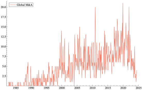
Figure 1.
Completed mergers and acquisitions (M&A) in the global water industry.
For this analysis, we utilized the daily number of completed M&A deals in the water sector to construct an aggregate monthly time series. By aggregating the data on a monthly basis, we aimed to capture the broader trends and waves of M&A activity in the water industry.
3. Methodology
3.1. Unit Roots
There are various approaches available for testing unit roots. In this study, we utilized the Augmented Dickey–Fuller (ADF) test proposed by [36]. Alternative methods, such as the procedure developed by [37], which relies on a non-parametric estimation of the spectral density of at the zero frequency, can also be applied to improve the power of unit root tests. Furthermore, this analysis incorporates techniques introduced by [38] and [39]. These approaches, especially when considering deterministic trends, generally produce comparable outcomes.
3.2. ARFIMA (p, d, q) Model
Building on the work of scholars such as [40,41,42], it is now well-recognized that standard unit root tests exhibit very low power when the underlying data-generating process is fractionally integrated or characterized by long memory. To account for this, fractional differentiation orders are considered in the analysis.
Consequently, this study employed the ARFIMA (p, d, q) model, described by the following equation:
In formulation, is assumed to follow an process, meaning it is a covariance stationary process with a constant mean and variance, as well as a spectral density that is strictly positive at frequency zero. is the lag operator , represents a fractional differentiation parameter, and is a time series integrated of order .
The selection of appropriate AR and MA orders for the model was guided by the Bayesian Information Criterion ([43]) and Akaike Information Criterion ([44]). For both the full time series and its subsamples, the parameter d was estimated across all viable combinations of AR and MA terms , with 95% confidence intervals applied to validate the estimates.
3.3. Markov-Switching Dynamic Regression (MS-DR) Model
Our approach is based on the single-index Markov-switching dynamic factor model, which combines co-movements and business-cycle shifts into a statistical model and was first developed in the mid-1990s by [45,46,47]. According to the model, a vector of economic indicators, , which are assumed to fluctuate in tandem with the state of the economy generally, can be broken down into the total of two parts. The common comovements are explained by the first component, , which is a linear combination of unseen factors.
The time series vector , which depicts the peculiar movements in the series, is the second element. This implies the following formulation:
where is the vector of idiosyncratic components and is the factor loading matrix.
We explain the business cycle asymmetries by supposing that an unobserved regime-switching state variable, , controls the dynamic behavior of the common factors. The expansion and recession states at time t can be denoted by the labels amd , respectively, in this paradigm. Furthermore, the conventional wisdom holds the state variable changes in accordance with an irreducible two-state Markov chain, the transition probabilities of which are determined by
where , and represents the information set up to period . It is assumed that the common factor vector is subject to an autoregressive process with a switching intercept
where is an independent variable of white noise with variance . The basic idea that the comovements of the various time series originate from the common component is expressed by the primary identifying assumption in the model. By presuming that and are mutually uncorrelated at all leads and lags, this is accomplished (this theoretical section does not address additional identifying restrictions that are needed to estimate the model).
The idiosyncratic error is assumed to have an autoregressive process of order for each element .
where a white noise process with variance is represented by . The idiosyncratic component’s dynamics are expressed in matrix form as
where , , and (finding the common factors in small-scale factor models requires assuming that the idiosyncratic components are uncorrelated in cross-section ([48]); it is assumed that the idiosyncratic mistakes in large-scale models (N → ∞) have a weak correlation).
This model is particularly suitable for capturing nonlinearities and structural shifts in time series data, as it allows the parameters governing both the common factors and idiosyncratic components to change according to latent regimes. The Markov-switching structure enables the model to distinguish between different economic phases, such as expansion and contraction, making it highly appropriate for analyzing M&A activity that may respond asymmetrically to macroeconomic cycles. Moreover, by incorporating a dynamic factor approach, the model effectively isolates common trends from firm-specific or sector-specific shocks, thus providing a more refined understanding of the underlying economic forces.
4. Empirical Results
The unit root/stationarity test is the first study we performed in this research article to examine the global water industry, covering the period from September 1982 to June 2024. We used the Kwiatkowski–Phillips–Schmidt–Shin (KPSS) test, the Phillips Perron (PP) test, and the Augmented Dickey–Fuller (ADF) test to analyze the data and determine if the time series are non-stationary I(1) or stationary I(0). This is crucial for data analysis since it makes it possible to interpret the model parameters more consistently. The results can be distorted by a trend or seasonal volatility, which can lead to incorrect inferences about the underlying relationships in the data.
Table 1 presents the results derived from the unit root tests. The outcomes reveal that the time series did not exhibit a clear I(0) stationary or I(1) non-stationary behavior. While the ADF and PP tests suggest that the series was stationary, the KPSS test indicates otherwise, showing a stochastic rather than deterministic trend. This implies that the deviations from the mean in the completed M&As were not corrected automatically over time. Instead, each future value depended on the previous one plus an error term, leading to the accumulation of past errors. To address this issue, we reanalyzed the series using first differences, resulting in an I(0) behavior. This outcome aligns with expectations, as the aforementioned methods only account for integer differentiation degrees, such as 0 for stationary series and 1 for non-stationary series. Consequently, in subsequent analysis, we introduced greater flexibility by allowing fractional differentiation, as implemented in the ARFIMA approach.

Table 1.
Unit root tests.
Given the lower power of unit root tests under fractional alternatives, we further applied fractionally integrated techniques, employing ARFIMA (p, d, q) models to explore persistence in mergers and acquisitions within the water sector.
The Akaike Information Criterion (AIC; [44]) and Bayesian Information Criterion (BIC; [43]) are used to determine the optimal AR and MA orders for the models. However, caution is warranted, as these criteria may not always be the most reliable for fractional models [49,50].
The ARFIMA (p, d, q) models offer several advantages over traditional unit root tests: (1) they accommodate fractional values of dd, providing greater modeling flexibility; (2) they capture long-term dependencies; and (3) they offer a comprehensive framework for time series modeling and forecasting.
Table 2 provides the estimates of the fractional differencing parameter dd and the AR and MA terms, calculated using [51] maximum likelihood estimator for various ARFIMA (p, d, q) specifications, considering all combinations of for each time series.
Table 2.
Long memory results using the original time series.
We observe from Table 2 that the estimates of what we obtained by focusing on the original time series of mergers and acquisitions in the water sector was lower than 0.5 . According to this result, we can determine that since the result of parameter d was 0.33, the series had a stationary behavior and supported a mean reversion behavior that implied transitory shocks. That is, in the face of an exogenous shock, the series will return to its original trend in the future.
Once we fitted the best ARFIMA time series model exhibited in Table 2, we performed the Brock, Dechert, and Scheinkman (BDS) nonparametric test using the residual values of the fitted ARFIMA model in order to hypothesize about the independence and identical distribution of the data.
The hypotheses used to determine the linearity or nonlinearity of the data are as follows:
H0.
The information is uniformly and independently dispersed (I.I.D.).
H1.
The time series is non-linearly dependent as the data are not I.I.D.
Table 3 displays the estimates of the BDS test for the fitted model, ARFIMA (0, d, 0).
Table 3.
Test of the time independence of the water sector.
As can be seen from Table 3, three different embedding dimensions (it represents the dimension of the space in which the trajectories of the time series are evaluated) and four different epsilon values (used to determine whether points in the embedded space are close to each other) were used in the BDS test procedure to obtain the BDS statistics (that show how far away the series is from being i.i.d.).
All test values were statistically significant at the 95% confidence level. Therefore, we rejected the null hypothesis in favor of the alternative. This fact suggests the existence of nonlinear structures in the data.
Next, we performed a logarithmic transformation of the original data in order to liberalize the data and we used the ARFIMA models again to obtain the new results for our long memory analysis.
Table 4 displays the estimates of the fractional differencing parameter d and the AR and MA terms for the transformed time series in logs.
Table 4.
Long memory results using the time series in logs.
Table 4 presents the new results with the original data transformed into logarithms. The results are quite similar to the previous ones, where the value of the parameter suggests the existence of long memory and mean reversion behavior in the face of exogenous shocks.
To determine whether the log-transformed data and the new ARFIMA model chosen for the AIC and BIC criteria achieved linearity, we recalculated the BDS test. The results are shown in Table 5.
Table 5.
Test of the time independence of the water sector with the differenced series.
According to the results presented in Table 5, with the differenced time series, again we found evidence of nonlinearity effects. That is, the probability was less than 5% at the significance level, implying a rejection of the null hypothesis that the stock returns series is linearly dependent.
Due to the results, we presented previously and in order to capture nonlinear behaviors associated with abrupt changes in a time series, we followed the methodology presented by [52], a Markov Switching (MS) model.
Table 6 shows the estimates of the Markov-switched dynamic regression model using the maximum likelihood method.
Table 6.
Estimation of the MS (2) dynamic regression model.
The adjusted model refers to the MS (2), which means that the model assumes two possible regimes: (intense M&A activity) or (“normal” M&A activity). In section 1 of Table 6, we present the descriptive statistics for residuals. In the normality test, the value obtained was significant at 5% and 1%, respectively. This result indicates that the data did not follow a normal distribution. On the other hand, according to the ARCH 1-1 test, it was observed that the variance of the errors was constant over time and that its behavior did not depend on past observations.
For the Ljung–Box or Portmanteau test (36), the null hypothesis was again rejected in favor of the alternative. This means that there was autocorrelation (the series was not random) in at least 1 of the first 36 lags.
Finally, the LR–test for linearity indicates that the result was again significant and suggests that a nonlinear model provides a better representation of the data.
In Section 2 of Table 6, we present the results from the Markov-switching model that we estimated. It is noted that each of the regime-specific values and intercepts obtained from the time series (constant for each regime) served as an indicator to determine the average growth rate of M&As in the water sector for a specific regime. The results indicate two markedly distinct regimes. As we can see in states of high M&A intensity, we obtained a result of 7.46; while for a state of normal M&A activity, it was 1.61, and there was a deviation with respect to these estimates (sigma) of 2.86.
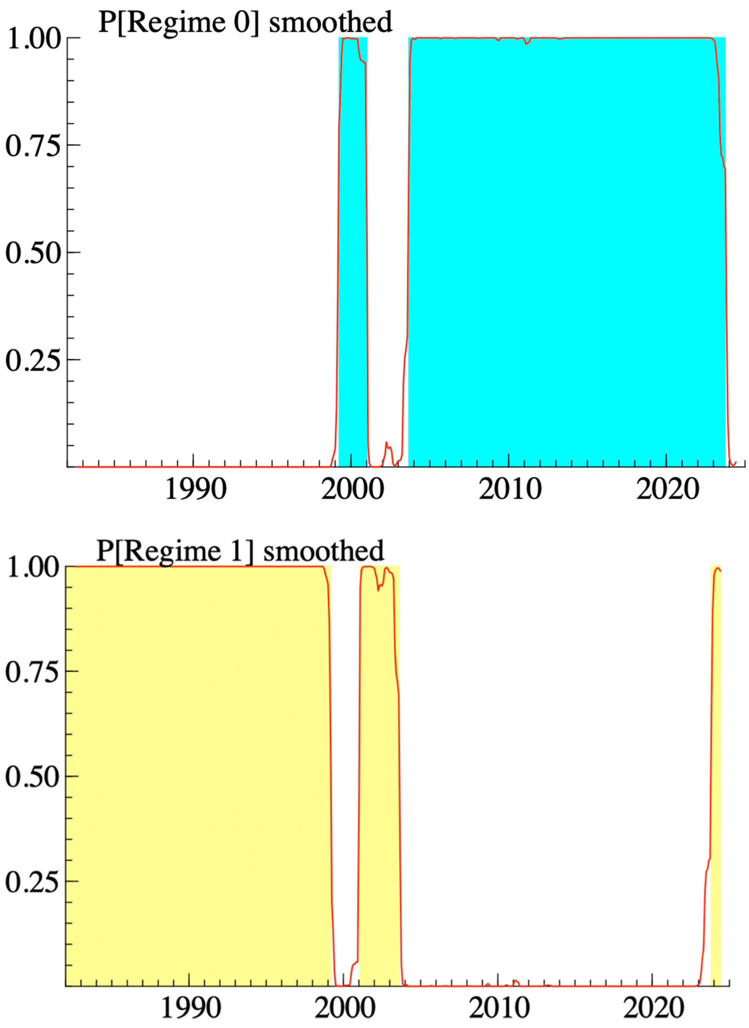
In Section 3 of the Table 6, we placed the focus on the durations of each regime for the time series we were analyzing. To explain this section, we wanted to make it more visual in order to make it understandable. For this reason, we decided to represent the results obtained in this section in Figure 2.
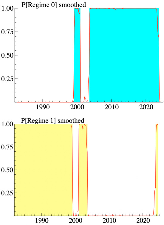
Figure 2.
Graphical representation of the regimes.
The upper panel presents the smoothed probabilities for the market in regime 0, and the lower panel presents the smoothed probabilities for the market in regime 1. From the estimated probabilities, the M&A in the water sector remained under the intense activity regime for two periods, totaling 264 months. In the regime of normal activity, the sector carried out mergers and acquisitions in three different periods, totaling 238 months.
Finally, we focused on the degree of persistence. Importantly, persistence seems to be an important characteristic of M&A, as shown by different studies for the US and the UK under different approaches (see [5,53,54]). In Section 4 of Table 6, we determined regime persistence (stability). In other words, if the economy is under a given regime, there is a probability of remaining in that regime. According to our results, regarding the transaction and persistence matrix of the regimes, it turns out that regime 0 was more persistent, i.e., the probability of remaining in this regime in a subsequent period was approximately 99.19%, and that of moving to regime 2 was of the order of 0.81%. In regime 2, the probability of continuing this regime in period t + 1 was 99.105%, while the probability of switching to regime 1 was 0.89%.
5. Concluding Remarks
This study provides an in-depth analysis of the cyclical patterns of mergers and acquisitions (M&A) in the global water sector, spanning the period from 1982 to 2024. By employing advanced econometric models, including ARFIMA and the Markov-switching dynamic regression (MS-DR) model, we were able to capture both the linear and nonlinear dynamics present in M&A activity. The findings offer valuable insights into the behavior of M&A waves, the persistence of activity regimes, and the role of external shocks in shaping the sector’s consolidation patterns.
Our results demonstrate that the water industry’s M&A activity exhibits stationary behavior, meaning that, in the face of exogenous shocks, the time series tends to revert to its original trend. This characteristic suggests a degree of resilience in the sector, where short-term disruptions are absorbed, allowing the market to return to its long-term trajectory. However, the application of the BDS test highlighted the presence of nonlinear dependencies, pointing to the complex and irregular nature of M&A cycles in the sector. This nonlinearity emphasizes the importance of accounting for sudden shifts and structural changes when analyzing M&A behavior.
The MS-DR model further revealed that once the water industry enters a high-activity M&A regime, it tends to remain in this state for prolonged periods. This persistence suggests that external factors, such as regulatory changes, technological advancements, or global water scarcity, are key drivers in sustaining M&A waves. Such factors create opportunities for consolidation and restructuring, as companies seek to strengthen their positions in a highly competitive and resource-constrained environment.
These findings have important implications for both policymakers and industry stakeholders. The stationary yet cyclical nature of M&A activity indicates that strategic interventions, whether regulatory or market-driven, can have long-lasting effects on the industry’s structure. Policymakers should carefully consider the timing and scope of regulatory reforms, as these could either amplify or mitigate waves of consolidation. For corporate strategists, understanding the persistence of high-activity regimes can inform decisions on market entry, mergers, and acquisitions, helping firms navigate periods of intense competition more effectively.
Author Contributions
Conceptualization, M.M.; Methodology, M.M.; Software, M.M.; Formal analysis, M.M.; Investigation, M.M., R.H. and J.I.; Data curation, M.M.; Writing—Original draft, M.M., R.H. and J.I.; Writing—review & editing, M.M., R.H. and J.I.; Visualization, M.M., R.H. and J.I.; Supervision, M.M. All authors have read and agreed to the published version of the manuscript.
Funding
This research received no external funding.
Data Availability Statement
The data employed in this research paper is downloaded from Thomson Reuters Eikon database. The data that support the findings of this study are available on request from the corresponding author. The data are not publicly available due to privacy or ethical restrictions.
Conflicts of Interest
The authors declare no conflict of interest.
References
- Kolev, K.; Haleblian, J.; McNamara, G. A review of the merger and acquisition wave literature: History, antecedents, consequences and future directions. In The Handbook of Mergers and Acquisitions; Oxford University Press: Oxford, UK, 2012; pp. 19–39. [Google Scholar]
- Martynova, M.; Renneboog, L. Spillover of corporate governance standards in cross-border mergers and acquisitions. J. Corp. Financ. 2008, 14, 200–223. [Google Scholar] [CrossRef]
- Freier, J. Successful Corporate Acquisitions: A Complete Guide for Acquiring Companies for Growth and Profit; Prentice Hall, Inc.: Eng-lewood Cliffs, NJ, USA, 1990; 401p, ISBN 0138605033. [Google Scholar]
- Town, R.J. Merger waves and the structure of merger and acquisition time-series. J. Appl. Econ. 1992, 7, S83–S100. [Google Scholar] [CrossRef]
- Barkoulas, J.T.; Baum, C.F.; Chakraborty, A. Waves and persistence in merger and acquisition activity. Econ. Lett. 2001, 70, 237–243. [Google Scholar] [CrossRef]
- Coase, R. The nature of the firm. In The Economic Nature of the Firm: A Reader; Kroszner, R.S., Putterman, L., III, Eds.; Cambridge University Press: Cambridge, UK, 2009; pp. 79–95. [Google Scholar]
- Nelson, R.L. Merger Movements in American Industry: 1895–1956; University Microfilms: Ann Arbor, MI, USA, 1966. [Google Scholar]
- Gort, M. An economic disturbance theory of mergers. Q. J. Econ. 1969, 83, 624–642. [Google Scholar] [CrossRef]
- Mitchell, M.L.; Mulherin, J.H. The impact of industry shocks on takeover and restructuring activity. J. Financ. Econ. 1996, 41, 193–229. [Google Scholar] [CrossRef]
- Shleifer, A.; Vishny, R.W. Equilibrium short horizons of investors and firms. Am. Econ. Rev. 1990, 80, 148–153. [Google Scholar]
- Harford, J. What drives merger waves? J. Financ. Econ. 2005, 77, 529–560. [Google Scholar] [CrossRef]
- Rouzies, A.; Coleman, H.; Angwin, D.N. Distorted and adaptive integration: Realized post-acquisition integration as embedded in an ecology of processes. Long Range Plan. 2019, 52, 271–282. [Google Scholar] [CrossRef]
- Thanos, I.C.; Papadakis, V.M.; Angwin, D. Does changing contexts affect linkages throughout the mergers and acquisition process? A multiphasic investigation of motives, pre-and post-acquisition and performance. Strateg. Change 2020, 29, 149–164. [Google Scholar] [CrossRef]
- World Economic Forum Annual Meeting (2009). The Bubble Is Close to Bursting: A Forecast of the Main Economic and Geo-political Water Issues Likely to Arise in the World During the Next Two Decades. Available online: https://calisphere.org/item/ark:/86086/n2rb73j9/ (accessed on 27 March 2025).
- Marques, R.; Carvalho, P.; Pires, J.; Fontainhas, A. Willingness to pay for the water supply service in Cape Verde–how far can it go? Water Sci. Technol. Water Supply 2016, 16, 1721–1734. [Google Scholar] [CrossRef]
- Laffont, J.J. Regulation and Development; Cambridge University Press: Cambridge, UK, 2005. [Google Scholar]
- Molinos-Senante, M.; Hernández-Sancho, F.; Sala-Garrido, R. Economic feasibility study for wastewater treatment: A cost–benefit analysis. Sci. Total Environ. 2010, 408, 4396–4402. [Google Scholar] [PubMed]
- Marques, R.C.; Simões, P.; Pires, J.S. Performance benchmarking in utility regulation: The worldwide experience. Pol. J. Environ. Stud. 2011, 20, 125–132. [Google Scholar]
- Mikulik, J.; Babina, M. The Role of Universities in Environmental Management. Pol. J. Environ. Stud. 2009, 18, 527–531. [Google Scholar]
- Correia, T.; Marques, R.C. Performance of Portuguese water utilities: How do ownership, size, diversification and vertical integration relate to efficiency? Water Policy 2011, 13, 343–361. [Google Scholar]
- Pinto, F.S.; Simões, P.; Marques, R.C. Raising the bar: The role of governance in performance assessments. Util. Policy 2017, 49, 38–47. [Google Scholar] [CrossRef]
- Abbott, M.; Cohen, B.; Wang, W.C. The performance of the urban water and wastewater sectors in Australia. Util. Policy 2012, 20, 52–63. [Google Scholar]
- Hana, U. Competitive advantage achievement through innovation and knowledge. J. Compet. 2013, 5, 82–96. [Google Scholar]
- Berg, S.; Marques, R.C. Quantitative studies of water and sanitation utilities: A benchmarking literature survey. Water Policy 2011, 13, 591–606. [Google Scholar] [CrossRef]
- Carvalho, P.; Marques, R.C.; Berg, S. A meta-regression analysis of benchmarking studies on water utilities market structure. Util. Policy 2012, 21, 40–49. [Google Scholar]
- Worthington, A.C. A review of frontier approaches to efficiency and productivity measurement in urban water utilities. Urban Water J. 2014, 11, 55–73. [Google Scholar]
- Gugler, K.; Konrad, K.A. Merger Target Selection and Financial Structure; University of Vienna and Wissenschaftszentrum Berlin (WZB): Berlin, Germany, 2002. [Google Scholar]
- Hoberg, G.; Phillips, G. Product market synergies and competition in mergers and acquisitions: A text-based analysis. Rev. Financ. Stud. 2010, 23, 3773–3811. [Google Scholar]
- Cho, S.; Chung, C.Y. Review of the literature on merger waves. J. Risk Financ. Manag. 2022, 15, 432. [Google Scholar]
- Monge, M. The financial market wants to believe in European sustainability. Time trends and persistence analysis of green vs. brown bond yields. Environ. Sci. Adv. 2024, 3, 1452–1463. [Google Scholar]
- Ceron, B.M.; Monge, M. Luxury goods and services in recession periods. Time trends and persistence analysis. J. Revenue Pricing Manag. 2024, 23, 588–595. [Google Scholar]
- Monge, M.; Gil-Alana, L.A. Fractional integration and cointegration in merger and acquisitions in the US petroleum industry. Appl. Econ. Lett. 2016, 23, 701–704. [Google Scholar]
- Monge, M.; Gil-Alana, L.A.; Perez de Gracia, F.; Rodriguez Carreno, I. Are mergers and acquisitions in the petroleum industry affected by oil prices? Energy Sources Part B Econ. Plan. Policy 2017, 12, 420–427. [Google Scholar]
- Monge, M.; Gil-Alana, L.A.; Cristobal, E. Mergers and acquisitions in the lithium industry. A fractional integration analysis. Rev. Dev. Financ. 2020, 10, 31–37. [Google Scholar]
- Monge, M.; Cristobal, E.; Gil-Alana, L.A. How lithium prices affect mergers and acquisitions in the lithium industry. Rev. Dev. Financ. 2021, 11, 26–34. [Google Scholar]
- Dickey, D.A.; Fuller, W.A. Distributions of the estimators for autoregressive time series with a unit root. J. Am. Stat. Assoc. 1979, 74, 427–481. [Google Scholar]
- Phillips, P.C.B.; Perron, P. Testing for a unit root in time series regression. Biometrika 1988, 75, 335–346. [Google Scholar]
- Kwiatkowski, D.; Phillips, P.C.; Schmidt, P.; Shin, Y. Testing the null hypothesis of stationarity against the alternative of a unit root. J. Econom. 1992, 54, 159–178. [Google Scholar]
- Elliot, G.; Rothenberg, T.J.; Stock, J.H. Efficient tests for an autoregressive unit root. Econometrica 1996, 64, 813–836. [Google Scholar]
- Lee, D.; Schmidt, P. On the power of the KPSS test of stationarity against fractionally-integrated alternatives. J. Econom. 1996, 73, 285–302. [Google Scholar]
- Hassler, U.; Wolters, J. On the power of unit root tests against fractional alternatives. Econ. Lett. 1994, 45, 1–5. [Google Scholar]
- Diebold, F.X.; Rudebush, G.D. On the power of Dickey-Fuller tests against fractional alternatives. Econ. Lett. 1991, 35, 155–160. [Google Scholar]
- Akaike, H. A Bayesian extension of the minimum AIC procedure of autoregressive model fitting. Biometrika 1979, 66, 237–242. [Google Scholar]
- Akaike, H. Maximum likelihood identification of Gaussian autoregressive moving average models. Biometrika 1973, 60, 255–265. [Google Scholar]
- Chauvet, M. An econometric characterization of business cycle dynamics with factor structure and regime switches. Int. Econ. Rev. 1998, 39, 969–996. [Google Scholar]
- Kim, C.; Nelson, C. Business cycle turning points, a new coincident index, and tests of duration dependence based on a dynamic factor model with regime switching. Rev. Econ. Stat. 1998, 80, 188–201. [Google Scholar]
- Kim, C.; Yoo, J.S. New index of coincident indicators: A multivariate Markov switching factor model approach. J. Monet. Econ. 1995, 36, 607–630. [Google Scholar]
- Barhoumi, K.; Darne, O.; Ferrara, L. Dynamic factor models: A review of the literature. J. Bus. Cycle Meas. Anal. 2014, 8, 73–107. [Google Scholar]
- Hosking, J.R. Modeling persistence in hydrological time series using fractional differencing. Water Resour. Res. 1981, 20, 1898–1908. [Google Scholar]
- Beran, J.; Bhansali, R.; Ocker, D. On unified model selection for stationary and nonstationary short- and long-memory autoregressive processes. Biometrica 1998, 85, 921–934. [Google Scholar]
- Sowell, F. Maximum likelihood estimation of stationary univariate fractionally integrated time series models. J. Econ. 1992, 53, 165–188. [Google Scholar]
- Hamilton, J. A new approach to the economic analysis of nonstationary time series and the business cycles. Econometrica 1989, 57, 357–384. [Google Scholar]
- Resende, M. Mergers and acquisitions in the UK: A disaggregated analysis. Appl. Econ. Lett. 1996, 3, 637–640. [Google Scholar]
- Resende, M. Wave Behaviour of Mergers and Acquisitions in the UK: A Sectoral Study. Oxf. Bull. Econ. Stat. 1999, 61, 85–94. [Google Scholar]

Disclaimer/Publisher’s Note: The statements, opinions and data contained in all publications are solely those of the individual author(s) and contributor(s) and not of MDPI and/or the editor(s). MDPI and/or the editor(s) disclaim responsibility for any injury to people or property resulting from any ideas, methods, instructions or products referred to in the content. |
© 2025 by the authors. Licensee MDPI, Basel, Switzerland. This article is an open access article distributed under the terms and conditions of the Creative Commons Attribution (CC BY) license (https://creativecommons.org/licenses/by/4.0/).