Abstract
The study constructed a supply chain inventory model for sellers and buyers that integrates payment-time-dependent demand, product defects, misclassification risks, and carbon emission tax considerations. The model was designed to optimize payment time, replenishment time, and order quantities to maximize the seller’s profit per unit time. Theoretical analysis showed that profit exhibited joint concavity with respect to both payment time and replenishment time. An algorithm was also formulated to derive optimal solutions. Finally, numerical experiments and sensitivity analyses validated the model and offered practical insights for managing inventories involving imperfect products. Results indicated that higher responsiveness of demand to payment timing, greater demand coefficients, better product prices, and higher scrap values led to increased seller profits, while greater misclassification, credit default risks, and carbon tax rate reduced it. These insights help decision-makers select suitable parameter values for efficient operations.
MSC:
90B06
1. Introduction
The traditional economic order quantity (EOQ) model often assumes that all products provided by suppliers are of perfect quality, which is unrealistic. In reality, defects inevitably occur due to imperfections in production or transportation processes. Such defective products can affect inventory levels, customer service standards, and order frequency within the inventory system. Therefore, it is necessary to analyze the impact of defective products on inventory systems. Through screening processes, defective items can be identified; however, such processes may result in incorrect inspection results due to human negligence, inspection machine failure, improper inspection methods, or other factors. Misclassifying good products as defective constitutes a type I error, leading to profit loss, whereas treating defective items as good constitutes a type II error, incurring penalty costs.
Many studies have discussed the impacts of product quality defects and inspection errors on inventory systems. Paknejad et al. [1] considered the quantity of defective items in a lot as a random variable and analyzed its effect on operational performance. Salameh and Jaber [2] modified the traditional EOQ model by incorporating imperfect-quality items, which were collected and sold as a single batch after the inspection process. Focusing on profit maximization, Yoo et al. [3] formulated an inventory model for imperfect-quality products that included two types of inspection errors and defective item returns. The model addressed reverse logistics, as well as customer returns due to type II errors. It also incorporated reworking and salvaging processes for items misclassified due to type I errors.
Wang et al. [4] examined the integration of input material acquisition, material inspection, and production planning, considering cases with type I and type II inspection errors, where the unit acquisition cost varied based on the average quality level. Rezaei [5] combined an EOQ model with sampling inspection strategies for handling imperfect items. An integrated production-inventory model incorporating a defective item-dependent stochastic credit period was introduced by Das et al. [6]. Manna et al. [7] developed an inventory model for imperfect production, where the defective rate was influenced by the production rate, and demand was affected by advertisement. Sarkar and Giri [8] introduced a supply chain model incorporating stochastic elements, an imperfect production process, and a controllable defect rate.
Hauck et al. [9] proposed a model aimed at maximizing profit by incorporating quality inspection, pricing strategies, and lot sizing decisions for a single imperfect-quality product. Karakatsoulis and Skouri [10] investigated how to optimize reorder levels and lot sizes in an inventory system where defective items were present. Hauck et al. [11] focused on a two-stage supply chain featuring imperfect-quality products, where the screening time directly affected the batch quality, cost considerations, and consumer demand. Various research papers have been published on the topics of product quality and lot sizing, such as those by Jaber et al. [12], Mondal et al. [13], Lin [14], Sana [15], Sarker et al. [16], Khan et al. [17], Sarker and Moon [18], Sarkar and Saren [19], Yu and Hsu [20], Pal and Mahapatra [21], Hauck et al. [22], Beranek and Buscher [23], and their references.
On January 15, the World Economic Forum (WEF) issued The Global Risks Report 2025, which ranked “extreme weather events” as the second most probable short-term (2-year) risk and the top long-term (10-year) risk among the 10 major global threats. It is well recognized that carbon dioxide (CO2) emissions play a crucial role in accelerating climate change, with their impact growing more severe each year. The increasing frequency of extreme weather events has heightened awareness of the greenhouse effect and global warming. In response to these challenges, governments worldwide are focusing on minimizing carbon emissions from industrial processes. Key strategies include advancing renewable energy adoption, enforcing energy conservation and emission reduction policies, creating carbon trading frameworks, introducing carbon taxation, and leveraging carbon offset solutions. These initiatives are expected to bring significant changes to business operations and corporate sustainability efforts.
The concept of a green supply chain emphasizes the integration of sustainability and environmental considerations into production and service operations. Given the critical role of carbon emissions in climate change and ecological degradation, minimizing them is a primary focus within this framework. Carbon reduction efforts are largely guided by two regulatory approaches: cap-and-trade systems and carbon taxation. These policies have sparked growing research interest in their impact on operational management, reinforcing the need for carbon-conscious inventory strategies. Consequently, production and inventory models now increasingly incorporate carbon reduction strategies.
Dye and Yang [24] proposed an inventory model for deteriorating items that considered various carbon emission policies. They also explored the impact of trade credit risk, aiming to find the optimal credit period and replenishment strategy to maximize the retailer’s total profit. Daryanto et al. [25] explored a three-echelon supply chain model that integrated considerations for both carbon emissions and product deterioration. A study by Jain et al. [26] introduced a three-echelon supply chain inventory model that accounted for different carbon emission control policies, including taxation, offset strategies, and cap-and-trade regulations. Chang and Tseng [27] proposed inventory models for perishable products, taking into account scenarios where suppliers implemented advance-cash-credit payment strategies, customers engaged in cash-credit transactions, and carbon regulations (e.g., carbon taxes and cap-and-trade) were enforced. Their research focused on maximizing the expected total profit while incorporating carbon emission factors. The topic of carbon emissions reduction has been widely examined in various studies, such as those by Sabzevar et al. [28], Shi et al. [29], An et al. [30], Lu et al. [31], Fu et al. [32], Shi et al. [33], and He and Sun [34].
In contemporary markets with intense competition, sellers generally offer three different payment options:
- (1)
- Advance payment—buyers pay in full before receiving the goods or services.
- (2)
- Cash payment—buyers pay upon receiving the goods or services.
- (3)
- Credit payment—buyers are granted a delay payment period by the seller.
Advance payment plans help demonstrate the buyer’s creditworthiness while minimizing the risk of order cancellations. As a result, sellers can achieve greater accuracy in demand estimation. By offering credit payment options, sellers can increase sales without triggering price wars among competitors, making it an effective alternative to price discounts. Consequently, trade credit remains a widely used financial strategy in business operations. However, offering trade credit may draw in financially risky buyers and increase the likelihood of moral hazard. Similarly, advance payment requirements can intensify uncertainty and moral hazard for sellers. Empirical studies have indicated that trade financing methods influence the impact of demand shocks and the liquidity of trading partners.
Scholars have thoroughly investigated the influence of payment methods on inventory management decisions. The first EOQ model incorporating a constant demand rate and permissible delay in payments was developed by Goyal [35]. Zhang [36] introduced an advance payment system that included a fixed pre-payment cost to minimize both time and financial costs. Following Goyal’s [35] research, many researchers have investigated related issues under more generalized conditions. Teng [37] refined Goyal’s [35] model by accounting for the gap between the selling price and the purchase cost, demonstrating that under certain circumstances, allowing delayed payments resulted in shorter replenishment intervals and smaller order quantities. Chang et al. [38] developed an EOQ model for perishable goods, incorporating supplier credit terms that depended on order quantity. Jaggi et al. [39] introduced an EOQ model where demand was influenced by credit terms under a permissible delay in payments. Thangam and Uthayakumar [40] extended their work by including both selling price and credit-linked demand in an EOQ model for perishable inventory. Maiti et al. [41] examined an inventory model that integrated advance payment with stochastic lead time. They further developed a model that considered both stochastic lead time and price-dependent demand while incorporating advance payment.
Ouyang and Chang [42] focused on an economic production quantity (EPQ) model that integrated an imperfect manufacturing process, permissible delay in payments, and full backlogging. Liao et al. [43] developed an optimal strategy for perishable goods with capacity limitations, considering a two-level trade credit system. Chang et al. [44] formulated an inventory model for retailers to examine how defective items and trade credits influenced replenishment decisions. Li et al. [45] focused on the optimal replenishment policy for sellers, comparing advance, cash, and credit payment options. Majumder et al. [46] introduced an EPQ model for deteriorating substitute items under trade credit conditions. Panda et al. [47] introduced a credit policy approach within a two-warehouse inventory system for deteriorating goods with price- and stock-dependent demand and partial backlogging. Bi et al. [48] investigated the retailer’s trade credit strategy and ordering policy with credit-dependent demand under two-level trade credit. Shi et al. [49] studied a retailer’s optimal strategy for a deteriorating item with increasing demand under different payment schemes. Chang et al. [50] constructed a perishable inventory model specifically for retailers, incorporating partial backlogging and assuming that suppliers adopted an advance-cash-credit payment method, while retailers provided a cash-credit payment option for consumers. Interesting and relevant studies related to payment schemes include those by Teng et al. [51], Chern et al. [52], Taleizadeh et al. [53], Yang and Chang [54], Taleizadeh [55], Wang et al. [56], Wu et al. [57], Chen and Teng [58], Teng et al. [59], Li et al. [60], Li et al. [45], Chang et al. [61], Li et al. [62], Zou and Tian [63], Li et al. [64], Lin et al. [65], Shi et al. [33], Chang and Tseng [27], and Tsao et al. [66].
From the above investigations, it is evident that the presence of imperfect-quality goods in a lot is unavoidable, and errors in the inspection process can result in misclassification, leading to additional costs. Under the premise of sustainable development and environmental protection, minimizing carbon emissions is a crucial responsibility for corporate operations and management and a key objective of the green supply chain. Carbon taxes are one of the main ways to reduce carbon emissions effectively. The credit payment has a significant effect on inventory management, with either supplier costs or buyer benefits. The advance payment scheme is a popular payment method to reduce default risks. Hence, the influences of different payment methods (advance payment, cash payment, or credit payment) on inventory management are not ignored in real business transactions.
To capture the practical issues of inventory management and real market behaviors in the context of a green supply chain, the study discusses how the seller should determine the payment method (i.e., payment time) from the above options. The proposed EOQ model incorporates replenishment time and order quantity such that the seller’s total profit per unit time is maximized when the demand function is linked to the payment time. It also considers imperfect-quality goods, inspection errors, and the impacts of a carbon tax. The paper thus develops an extended inventory model for a supply chain involving both a seller and a buyer, where demand depends on payment time, and factors such as imperfect products, misclassification, and carbon tax policies are considered. The goal is to determine optimal strategies for payment time, replenishment time, and order quantity to maximize the seller’s profit per time unit. A summary comparison of the relevant models is presented in Table 1. As shown in Table 1, prior research has not simultaneously addressed the topics of payment type, inspection error, and carbon policy, resulting in an incomplete representation of inventory management and transaction market dynamics. This study bridges this gap by incorporating all these factors into the proposed analytical model. In addition, the demand function is formulated as a function of payment timing, allowing for a more realistic and comprehensive depiction of current inventory and market conditions. The integration of these elements represents a key contribution to this research.

Table 1.
A brief review of the related literature.
This paper is structured into eight sections. Section 2 defines the notations and assumptions applied in the study. Section 3 describes the proposed models. Section 4 presents the theoretical results and the algorithm for obtaining the optimal solution. Section 5 demonstrates the developed algorithm and validates the models with numerical examples. Section 6 carries out a sensitivity analysis and discusses managerial insights. Section 7 presents the managerial implications derived from the analytical and numerical results and elucidates how these insights can inform and support strategic decision-making by practitioners. Finally, Section 8 concludes the study and proposes future research directions.
2. Notation and Assumptions
We use the following notation and assumptions to discuss the extended inventory model.
| Notation: | |
| Purchasing cost per item in dollars. | |
| Selling price per item of a good product in dollars, where | |
| Scrap price per item in dollars, i.e., selling price of a defective product, where . | |
| Payment time in unit time (a decision variable). | |
| Proportion of defective-quality items produced, where . | |
| Probability of classifying a good item as defective, i.e., probability of type I error. | |
| Probability of classifying a defective item as good, i.e., probability of type II error. | |
| Inspecting rate per unit time. | |
| Inspecting cost per item in dollars. | |
| Ordering cost per order in dollars. | |
| Penalty cost per item in dollars, i.e., cost of accepting a defective item. | |
| Price discount per item per unit time in dollars when an advance payment is adopted. | |
| Holding cost per item per unit time in dollars. | |
| Interest rate per unit time. | |
| CO2 emissions generated during the procurement of a single unit of a product. | |
| CO2 emissions generated during the inspection of a single unit of a product. | |
| CO2 emissions associated with keeping a single unit of inventory per unit of time. | |
| CO2 emissions generated during the ordering process. | |
| Unit carbon tax. | |
| Demand rate per unit time, where and . | |
| Rate of default risk, where , , , and . | |
| Order quantity for each cycle. | |
| Length of replenishment cycle in unit time (a decision variable). | |
| Total profit per unit time in dollars, where . | |
- Assumptions:
- (1)
- Shortages are not allowed.
- (2)
- As stated in Jaggi et al. [39], it is observed that the credit period offered by the retailer to customers has a positive impact on demand. Hence, the longer the credit period is, the greater the demand. Conversely, the earlier the advance payment is, the less demand. As a result, the demand rate is a function of the payment time . Specifically, , where and .There are three types of payment time. (i) is an advance payment, (ii) is a cash payment on delivery, and (iii) is a credit payment. The seller offers a price discount per unit time for attracting more buyers when the advance payment is adopted. Specifically, the selling price per item of a good product is if the payment time is less than zero and the advance payment is used.
- (3)
- Inspection should be conducted on all items to classify them as either good or defective. It is assumed that the quantity of good products is at least equal to the demand during the inspection period to avoid shortages. Specifically, .
- (4)
- Due to defects in some products, to ensure that the order quantity is sufficient, it is assumed that the quantity of good products is at least equal to the adjusted demand, which is equal to the actual demand plus the number of good products classified as defective. For the sake of simplicity, we only consider that the quantity of good products equals the adjusted demand. Specifically, .
- (5)
- Good items are sold at unit price in the general market. Each defective product is sold as scrap at a unit price of .
- (6)
- Due to type I error, some good products are classified as defective and sold at unit price , resulting in loss of revenue. This loss of revenue is the cost of rejecting these good products.
- (7)
- Due to type II error, some products sold to meet demand may be defective. The defective products will be returned to the seller later and will be destroyed. The seller pays compensation to the buyer. The penalty cost is the cost of accepting these defective products.
- (8)
- As stated in Li et al. [45], it is evident that a 30-year mortgage has a higher default risk than a 15-year mortgage. Likewise, the longer the credit period is, the higher the percentage that the buyer will not be able to pay off the debt obligation. In short, the longer the credit period is, the higher the default risk. As a result, the rate of default risk is a function of payment time. The default risk does not exist when an advance payment is adopted. Hence, it exists when . The longer the credit period is, the greater the risk of default. The default risk is zero when a cash payment is adopted, i.e., and . The default risk is 100% when a credit payment is adopted and payment time tends to infinity, i.e., and .
- (9)
- The carbon tax policy serves as a primary strategy for mitigating carbon emissions. This policy framework focuses solely on the taxation of total carbon emissions, with no consideration given to other factors or mechanisms, such as trading or allowances. The seller’s carbon emissions predominantly stem from a range of operational activities, including tasks like ordering, purchasing, inspecting, and storage.
- (10)
- The ending inventory is zero.
3. Proposed Models
From the above notations and assumptions, the total profit per unit time consists of the following elements:
- (a)
- The ordering cost ;
- (b)
- The purchasing cost ;
- (c)
- The inspecting cost ;
- (d)
- The holding cost = (see Figure 1);
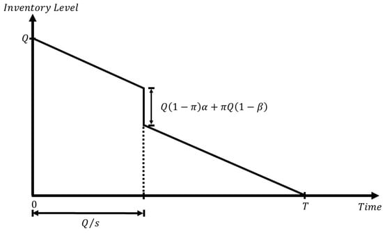 Figure 1. Graphical representation of the holding cost.
 - (e)
- The loss of revenue = ;
- (f)
- The penalty cost = ;
- (g)
- The carbon tax. The seller’s amount of CO2 emissions includes those from the buying, holding, inspecting, and ordering processes. Therefore, the carbon tax is equal to the unit carbon tax multiplied by the seller’s amount of CO2 emissions. Thus, the carbon tax amount is
- (h)
- The sales revenue;
- (i)
- The interest earned (lost).
Regarding (h) and (i), based on the value of , there are two cases: (1) and (2) 0.
- Case 1: (cash payment or advance payment)
For advance payment (i.e., < 0), the sales revenue includes revenue from good products and defective products. The seller provides price discount k for each good product to attract more customers. The interest earned is calculated by multiplying the revenue from good products (i.e., ) by the interest rate (i.e., ) and then by the prepayment period (i.e., ). Thus, the sales revenue and interest earned in case 1 are as follows:
- (h)
- The sales revenue = ;
- (i)
- The interest earned =
Hence, the total profit per unit time is
Case 2: 0 (cash payment or credit payment)
For credit payment (i.e., > 0), the sales revenue includes revenue from good products after the default risk and revenue from defective products. The interest lost is calculated by multiplying the revenue from good products (i.e., ) by the interest rate (i.e., ) and then by the credit period (i.e., ). Thus, the sales revenue and interest lost are obtained as follows:
- (h)
- The sales revenue = ;
- (i)
- The interest lost = .
Hence, the total profit per unit time for case 2 is obtained as
Note that if the cash payment system is adopted, = 0, and the total profit per unit time is
4. Theoretical Results
According to Assumption (4), we get . Specifically,
Case 1:
Substituting (5) into (2), we obtain
To maximize , we take the first- and second-order derivatives of in (6) with respect to T and , which leads to
and
Setting Equation (7) to zero to obtain a critical point and re-arranging terms, we obtain
Next, similarly setting Equation (8) to zero, we obtain
From Equations (12) and (13), the optimal replenishment time and payment time are determined to maximize .
Case 2:
Substituting (5) into (3), we obtain
To maximize , taking the first- and second-order derivatives of in (14) with respect to T and leads to
and
Setting Equation (15) to zero and re-arranging terms, we get
Next, setting Equation (16) to zero, we obtain
From Equations (20) and (21), the optimal replenishment time and payment time are determined to maximize .
Note that the corresponding Hessian matrix for the total profit per unit time
Using Equations (9) and (17), we obtain , for . Due to its complexity, it is difficult to show directly that the determinant of the Hessian matrix is positive (i.e., for ). Thus, we confirm the sufficient condition for the Hessian matrix to be negative-definite by applying Equations (9)–(11) and (17)–(19) and using Mathematica 13.1 with numerical examples. Moreover, the graphs of for are joint concave in and , shown in Examples 1 and 2 below.
Based on the above discussions and equations, we constructed a flowchart (Figure 2) and designed an Algorithm 1 to determine the optimal solution.
| Algorithm 1: Determine the Optimal Solution | |
| Step 0: Input the values of parameters. | |
| Step 1: Calculate and . | |
| Step 1.1 Step 1.2 Step 1.3 | Using Equations (12) and (13), obtain and . If , then substitute and into Equations (9)–(11) and calculate the determinant of the Hessian matrix . If , then substitute and into Equation (6) and calculate . Otherwise, . . |
| Step 2: Calculate . | |
| Step 2.1 Step 2.2 Step 2.3 | Using Equations (20) and (21), obtain and . If , then substitute and into Equations (17)–(19) and calculate the determinant of the Hessian matrix . If , then substitute and into Equation (14) and determine . Otherwise, . If . |
| Step 3: Set , and then the optimal solution is obtained. | |
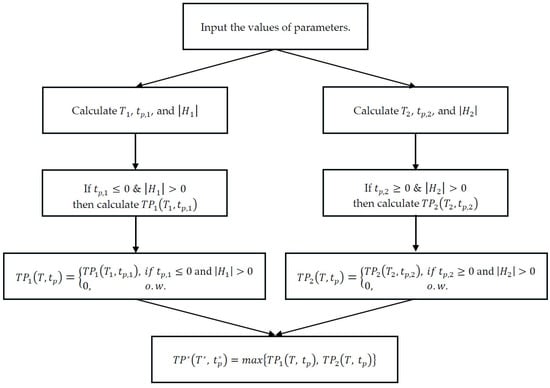
Figure 2.
Optimization algorithm process.
5. Numerical Examples
To demonstrate the effectiveness of the proposed model, flowchart, and algorithm under the study’s assumptions, several numerical examples are presented below to determine and analyze the optimal solutions.
From Assumption (2), the demand rate is an increasing function of the payment time. We discuss two types of . First, by following Jaggi et al. [39], Teng and Lou [67], Chen and Teng [58], and Li et al. [45], we assume , where , and is a coefficient of payment time . Then, we assume that is a linear function of , that is, , where , and is a slope of payment time . Additionally, from Assumption (8), the rate of default risk is a function of payment time; hence, by following Chern et al. [52], Wang et al. [56], Chen and Teng [58], and Li et al. [45], we assume that , where is the coefficient of default risk. According to the above two types of , we discuss the numerical example for the case of first and then for the other case of . Now, set the parameter values as and .
Type 1.
For .
Example 1.
Given
and , we obtain the following by applying the proposed algorithm using software Mathematica 13.1:
| Step | Hessian Matrix | ||
| 1 | |||
| 2 |
Hence, . The optimal payment time
years, the optimal replenishment time
years and the optimal total annual profit . Then, substitute
into Equations (1) and (5) to find the optimal carbon tax amount
and the optimal order quantity
units. Furthermore, the graph of
in (6), which is shown in Figure 3, clearly demonstrates that
exhibits joint concavity with both
and . The red point in Figure 3
presents the optimal solution . We note that the optimal payment time
is negative, and so advance payment is adopted.
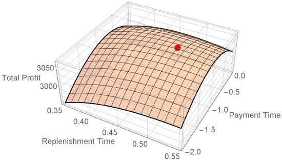
Figure 3.
Graphical representation of .
Example 2.
Given
and , we obtain the following using the proposed algorithm in software Mathematica 13.1: , ,
(because ), and
. Hence, . The optimal payment time
years, the optimal replenishment time
years, and the optimal total annual profit . Then, substitute
into Equations (1) and (5) to find the optimal carbon tax amount
and the optimal order quantity
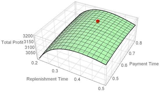
units. Furthermore, the graph of
in (14), which is shown in Figure 4, clearly demonstrates that
exhibits joint concavity with both T and . The red point in Figure 4
presents the optimal solution . Here, the optimal payment time
is positive, indicating that the credit payment is adopted.
Figure 4.
Graphical representation of .
Example 3.
Given
and , we obtain the following results: ,
and . Hence, . The optimal payment time , the optimal replenishment time
years and the optimal total annual profit . Then, substitute
into Equations (1) and (5) to find the optimal carbon tax amount
and the optimal order quantity
units. As the optimal payment time
is zero, cash payment is adopted.
Type 2.
For .
Example 4.
Let the parameter values be . Using the proposed algorithm and software Mathematica 13.1, we obtain the following results shown in Table 2.
Table 2.
Optimal solutions for .
We glean the following insights from Table 2:
- (1)
- When the slope of payment time is , the optimal payment time ; hence, advance payment is adopted.
- (2)
- When the slope of payment time is , the optimal payment time ; hence, cash payment is adopted.
- (3)
- When the slope of payment time is , the optimal payment time ; hence, credit payment is adopted.
- (4)
- The larger the slope is, the larger the optimal order quantity and the optimal carbon tax amount are, but the shorter the optimal replenishment time is.
- (5)
- The value of optimal total annual profit is smallest when cash payment is adopted.
6. Sensitivity Analysis
We used the parameter values from Example 2 to assess the impact of changes in input parameters on the optimal solution. The results of the sensitivity analysis are summarized in Table 3.
Table 3.
Sensitivity analysis for each parameter.
Table 3 reveals the following results:
- (1)
- As the coefficient of default risk increases, the optimal replenishment time also increases, whereas the optimal payment time , the optimal order quantity , the optimal carbon tax amount , and the optimal total annual profit all decrease. The impacts of the interest rate , the proportion of defective-quality items produced , the probability of type I error , the probability of type II error , the unit purchasing cost , the unit inspecting cost , and the unit penalty cost on the optimal solutions are identical to those of the coefficient of default risk on the optimal solutions . The analysis reveals that as parameters , , , , , , and increase, the decision-maker should extend the replenishment cycle, shorten the credit payment period, and reduce the order quantity. Consequently, both the optimal carbon tax amount and the total annual profit decrease.
- (2)
- A higher value of the coefficient of payment time leads to higher values of the optimal payment time , the optimal order quantity , the optimal carbon tax amount , and the optimal total annual profit but lower optimal replenishment time . The demand rate coefficient , the unit selling price of a good product p, and the unit scrap price w have the same impact on the optimal solutions as the coefficient of payment time . These results indicate that as parameters , b, p, and w increase, the decision-maker should shorten the replenishment cycle, extend the credit payment period, and increase the order quantity. Meanwhile, both the optimal carbon tax amount and the total annual profit increase.
- (3)
- When the holding cost (or the carbon emissions produced from holding ) increases, the optimal payment time , the optimal replenishment time , the optimal order quantity , the optimal carbon tax amount , and the optimal total annual profit all decrease. The analysis reveals that as parameters and increase, the decision-maker should shorten the replenishment cycle and the credit payment period and reduce the order quantity. At the same time, both the optimal carbon tax amount and the total annual profit decrease.
- (4)
- An increase in the unit carbon tax results in an increase in optimal replenishment time and optimal carbon tax amount but a decrease in the optimal payment time , the optimal order quantity , and the optimal total annual profit . The way (the carbon emission produced from the process of buying a unit product) and (the carbon emission produced from the process of inspecting a unit product) affect the optimal solutions is the same as how the unit carbon tax affects them. These results show that as parameters , , and increase, the decision-maker should extend the replenishment cycle, shorten the credit payment period, and decrease the order quantity. Meanwhile, the optimal carbon tax amount increases, but the total annual profit decreases.
- (5)
- The greater the value of (the carbon emission generated during the order process), the higher the values of the optimal replenishment time , the optimal order quantity , and the optimal carbon tax amount but the lower the values of the optimal payment time and the optimal total annual profit . The analysis indicates that as parameter increases, the decision-maker should extend the replenishment cycle, shorten the credit payment period, and increase the order quantity. At the same time, the optimal carbon tax amount increases, but the total annual profit decreases.
- (6)
- As the ordering cost grows, the optimal replenishment time and the optimal order quantity rise correspondingly, while the optimal payment time , the optimal carbon tax amount , and the optimal total annual profit decline. These results indicate that as parameter increases, the decision-maker should extend the replenishment cycle, shorten the credit payment period, and increase the order quantity. At the same time, both the optimal carbon tax amount and the total annual profit decrease.
- (7)
- When the inspecting rate increases, the optimal payment time , the optimal replenishment time , the optimal order quantity , the optimal carbon tax amount , and the optimal total annual profit all increase. The analysis shows that as parameter increases, the decision-maker should extend the replenishment cycle and the credit payment period and increase the order quantity. Meanwhile, both the optimal carbon tax amount and the total annual profit increase.
Since the price discount is solely associated with advance payment, we utilize the parameter values from Example 1 to analyze the sensitivity of the optimal solution to changes in . The results are shown in Table 4.
Table 4.
Sensitivity analysis for price discount .
As observed in Table 4, a greater price discount leads to an increase in the optimal order quantity and the optimal carbon tax amount while simultaneously reducing the optimal advance payment time and the optimal replenishment time . Additionally, the optimal total annual profit decreases. These results show that as parameter increases, the decision-maker should shorten the replenishment cycle, extend the credit payment period, and increase the order quantity. At the same time, the optimal carbon tax amount increases, but the total annual profit decreases.
7. Management Implications
Based on the findings from the “Numerical Examples” and “Sensitivity Analysis” Sections, the following managerial implications were identified, which can provide practical guidance for managers engaged in strategic decision-making and further illustrate the real-world applicability and value of employing inventory management and operations research methodologies.
- (1)
- The empirical evidence demonstrated that increases in misclassification probability, default risk coefficient, interest rate, proportion of defective items, unit purchasing cost, unit inspection cost, and unit penalty cost necessitated strategic adjustments wherein decision-makers should extend replenishment intervals, curtail credit payment periods, and reduce order quantities. Consequently, these adjustments precipitated a decline in both optimal carbon tax amounts and total annual profitability.
- (2)
- The analytical findings substantiated those elevations in payment time coefficient, demand rate coefficient, unit selling price of quality-conforming products, and unit scrap value and induced decision-makers to implement operational modifications including shortened replenishment cycles, extended credit periods, and increased order quantities. Concurrently, these strategic adaptations facilitated increases in both optimal carbon tax amounts and aggregate annual profit metrics.
- (3)
- The comprehensive analysis elucidated that incremental increases in holding costs or carbon emissions associated with inventory storage compelled decision-makers to adopt operational strategies characterized by shortened replenishment cycles, reduced credit payment periods, and diminished order quantities. These strategic recalibrations subsequently engendered decreases in both optimal carbon taxation levels and total annual profit margins.
- (4)
- The empirical investigation revealed that as unit carbon tax values and carbon emissions were attributable to procurement and inspection, decision-makers exhibited a propensity to extend replenishment cycles, contract credit periods, and decrease order quantities. These operational adjustments culminated in elevated optimal carbon tax amounts while simultaneously precipitating reductions in total annual profitability.
- (5)
- The research outcomes indicated that heightened carbon emissions per ordering event induced decision-makers to implement strategic modifications including extended replenishment cycles, increased order quantities, and reduced credit payment periods. Concomitantly, these adjustments resulted in elevated optimal carbon tax amounts while adversely affecting total annual profit metrics.
- (6)
- The empirical results demonstrated that increases in ordering costs necessitated strategic adaptations wherein decision-makers extended replenishment cycles, augmented order quantities, and reduced credit payment durations. Simultaneously, these operational modifications precipitated decreases in both optimal carbon tax amounts and total annual profitability.
- (7)
- The empirical investigation indicated that a higher inspection rate led the decision-maker to extend both the replenishment cycle and the credit payment period, while also increasing the order quantity. Concurrently, the optimal carbon tax and the total annual profit also exhibited an upward trend.
- (8)
- The empirical evidence suggested that incremental increases in price discount structures induced decision-makers to extend advance payment periods and augment order quantities while concurrently reducing replenishment cycle durations. These strategic adaptations resulted in elevated optimal carbon tax amounts, whereas total annual profitability experienced a concomitant decline.
8. Conclusions
We proposed an EOQ model that considered imperfect-quality product shipments, where demand was affected by payment time. This model aimed to determine the optimal payment time, replenishment schedule, and order quantity to maximize the seller’s total profit per unit time while accounting for misclassification and carbon tax. We derived the optimal solution by setting the first-order derivative of the total profit to zero. To confirm the concavity, we applied Mathematica 13.1 to verify that the Hessian matrix met the sufficient condition for being negative-definite. Graphs depicting total profit were used to demonstrate the joint concavity of payment time and replenishment time. Finally, we examined numerical examples, conducted sensitivity analyses, and presented management implications to provide a clearer understanding of the problem and key managerial implications.
With consideration for imperfect product shipments, classification errors, and carbon tax regulations, this study provides guidance on selecting optimal payment methods and replenishment strategies to enhance profitability. The main conclusions drawn from this research are summarized below.
- (1)
- When the probability of misclassification (type I or type II error) or the default risk coefficient rises, the optimal replenishment time increases, and the optimal credit payment time decreases, leading to a reduction in the optimal order quantity, carbon tax amount, and total profit. The interest rate, proportion of defective items, unit purchasing cost, unit inspection cost, and unit penalty cost exhibit similar effects on these optimal solutions. The findings suggest that when the probability of misclassification, default risk coefficient, interest rate, proportion of defective items, unit purchasing cost, unit inspection cost, and unit penalty cost increase, the decision-maker should extend the replenishment time, shorten the credit payment time, and reduce the order quantity. Consequently, both the optimal carbon tax amount and the total annual profit decline.
- (2)
- An increase in the coefficient of payment time results in a shorter optimal replenishment time; a longer optimal credit payment period; and an increase in the optimal order quantity, carbon tax amount, and total profit. These effects are also observed with changes in the demand rate coefficient, unit selling price of a good product, and unit scrap price. These findings indicate that increases in the payment time coefficient, demand rate coefficient, unit selling price of good-quality products, and unit scrap value lead the decision-maker to shorten the replenishment cycle, extend the credit period, and increase the order quantity. Concurrently, both the optimal carbon tax amount and total annual profit rise.
- (3)
- Higher holding costs or greater carbon emissions associated with inventory storage reduce the optimal replenishment time and credit payment time, subsequently lowering the optimal order quantity, carbon tax amount, and overall profit. The analysis reveals that increases in holding costs or carbon emissions related to inventory storage prompt the decision-maker to shorten the replenishment cycle and credit payment period, as well as reduce the order quantity. Consequently, both the optimal carbon tax amount and the total annual profit decline.
- (4)
- As the unit carbon tax rises, the optimal replenishment cycle extends, and the carbon tax amount increases, but the credit payment period shortens, ultimately lowering the optimal order quantity and total profit. These patterns also hold for carbon emissions associated with purchasing and inspecting a unit product. The results show that as the unit carbon tax and the carbon emissions from purchasing and inspecting each product rise, the decision-maker tends to lengthen the replenishment cycle, shorten the credit period, and decrease the order quantity. This leads to an increase in the optimal carbon tax amount and a reduction in total annual profit.
- (5)
- A higher level of carbon emissions per order leads to longer optimal replenishment time, larger order quantity, and higher carbon tax amount but results in a shorter optimal credit payment time and reduced total profit. The results suggest that an increase in carbon emissions per order causes the decision-maker to lengthen the replenishment cycle, raise the order quantity, and reduce the credit payment period. Simultaneously, the optimal carbon tax amount rises, while the total annual profit decreases.
- (6)
- When the ordering cost increases, both the optimal replenishment time and order quantity expand, whereas the optimal credit payment time, the optimal carbon tax amount, and total profit all decrease. The results show that an increase in ordering costs causes the decision-maker to lengthen the replenishment cycle, increase the order quantity, and reduce the credit payment period. Meanwhile, both the optimal carbon tax amount and total annual profit decrease.
- (7)
- A higher inspection rate contributes to increases in the optimal credit payment time, replenishment time, order quantity, carbon tax amount, and total profit. The results suggest that an increase in the inspection rate causes the decision-maker to lengthen the replenishment cycle and credit payment period, as well as raise the order quantity. At the same time, both the optimal carbon tax and total annual profit rise.
- (8)
- A larger price discount results in a higher optimal order quantity and carbon tax amount while shortening the optimal advance payment time and replenishment time. This also leads to a reduction in the total optimal profit. The results suggest that as price discounts increase, the decision-maker tends to extend the advance payment period and increase the order quantity, while shortening the replenishment cycle. Simultaneously, the optimal carbon tax amount rises, whereas the total annual profit declines.
These insights serve as a practical reference for managers in their strategic planning. Furthermore, they exemplify the tangible benefits of applying inventory management and operations research methodologies in real-world scenarios.
There are multiple ways to expand future research in this area. First, beyond carbon taxes, alternative carbon reduction policies, such as cap-and-trade or carbon offset, may influence sellers’ payment methods and replenishment strategies. Second, it could explore how carbon tax policies influence environmental regulations, sustainable development initiatives, and corporate social responsibility practices. Third, since product demand in modern markets is heavily impacted by selling price and advertising, future studies could incorporate these factors along with payment time in the demand function. Finally, expanding the research scope to include variables, such as perishable goods, random defect rate, and shortages, could provide further insights into payment method selection and inventory management.
Author Contributions
Conceptualization, C.-T.C. and Y.-T.T.; Methodology, C.-T.C. and Y.-T.T.; Software, Y.-T.T.; Formal analysis, C.-T.C.; Writing—original draft, C.-T.C.; Writing—review & editing, C.-T.C. and Y.-T.T.; Visualization, Y.-T.T. All authors have read and agreed to the published version of the manuscript.
Funding
This research received no external funding.
Data Availability Statement
Data sharing is not applicable to this article.
Conflicts of Interest
The authors declare no conflict of interest.
References
- Paknejad, M.J.; Nasri, F.; Affisco, J.F. Defective units in a continuous review (s,Q) system. Int. J. Prod. Res. 1995, 33, 2767–2777. [Google Scholar] [CrossRef]
- Salameh, M.K.; Jaber, M.Y. Economic production quantity model for items with imperfect quality. Int. J. Prod. Econ. 2000, 64, 59–64. [Google Scholar] [CrossRef]
- Yoo, S.H.; Kim, D.S.; Park, M.S. Economic production quantity model with imperfect-quality items, two-way imperfect inspection and sales return. Int. J. Prod. Econ. 2009, 121, 255–265. [Google Scholar] [CrossRef]
- Wang, C.H.; Dohi, T.; Tsai, W.C. Coordinated procurement/inspection and production model under inspection errors. Comput. Ind. Eng. 2010, 59, 473–478. [Google Scholar] [CrossRef]
- Rezaei, J. Economic order quantity and sampling inspection plans for imperfect items. Comput. Ind. Eng. 2016, 96, 1–7. [Google Scholar] [CrossRef]
- Das, B.C.; Das, B.; Mondal, S.K. An integrated production-inventory model with defective item dependent stochastic credit period. Comput. Ind. Eng. 2017, 110, 255–263. [Google Scholar] [CrossRef]
- Manna, A.K.; Dey, J.K.; Mondal, S.K. Imperfect production inventory model with production rate dependent defective rate and advertisement dependent demand. Comput. Ind. Eng. 2017, 104, 9–22. [Google Scholar] [CrossRef]
- Sarkar, S.; Giri, B.C. Stochastic supply chain model with imperfect production and controllable defective rate. Int. J. Syst. Sci. Oper. Logist. 2018, 5, 133–146. [Google Scholar] [CrossRef]
- Hauck, Z.; Rabta, B.; Reiner, G. Joint quality and pricing decisions in lot sizing models with defective items. Int. J. Prod. Res. 2021, 241, 108255. [Google Scholar] [CrossRef]
- Karakatsoulis, G.; Skouri, K. Optimal reorder level and lot size decisions for an inventory system with defective items. Appl. Math. Model. 2021, 92, 651–668. [Google Scholar] [CrossRef]
- Hauck, Z.; Rabta, B.; Reiner, G. Coordinating quality decisions in a two-stage supply chain under buyer dominance. Int. J. Prod. Res. 2023, 264, 108998. [Google Scholar] [CrossRef]
- Jaber, M.Y.; Bonney, M.; Moualek, I. An economic order quantity model for an imperfect production process with entropy cost. Int. J. Prod. Econ. 2009, 118, 26–33. [Google Scholar] [CrossRef]
- Mondal, B.; Bhunia, A.K.; Maiti, M. Inventory models for defective items incorporation marketing decisions with variable production cost. Appl. Math. Model. 2009, 33, 2845–2852. [Google Scholar] [CrossRef]
- Lin, T.Y. An economic order quantity with imperfect quality and quantity discounts. Appl. Math. Model. 2010, 34, 3158–3165. [Google Scholar] [CrossRef]
- Sana, S.S. A production inventory model in an imperfect production process. Eur. J. Oper. Res. 2010, 200, 451–464. [Google Scholar] [CrossRef]
- Sarker, B.; Sana, S.S.; Chaudhuri, K.S. Optimal reliability, production lot size and safety stock in an imperfect production system. Int. J. Math. Oper. Res. 2010, 2, 467–490. [Google Scholar] [CrossRef]
- Khan, M.; Jaber, M.Y.; Bonney, M. An economic order quantity (EOQ) for items with imperfect quality and inspection errors. Int. J. Prod. Econ. 2011, 133, 113–118. [Google Scholar] [CrossRef]
- Sarker, B.; Moon, I. An EPQ model with inflation in an imperfect production system. Appl. Math. Comput. 2011, 217, 6159–6167. [Google Scholar] [CrossRef]
- Sarkar, B.; Saren, S. Product inspection policy for an imperfect production system with inspection errors and warranty cost. Eur. J. Oper. Res. 2016, 248, 263–271. [Google Scholar] [CrossRef]
- Yu, H.F.; Hsu, W.K. An integrated inventory model with immediate return for defective items under unequal-sized shipments. J. Ind. Prod. Eng. 2016, 34, 70–77. [Google Scholar] [CrossRef]
- Pal, S.; Mahapatra, G.S. A manufacturing-oriented supply chain model for imperfect quality with inspection errors, stochastic demand under rework and shortages. Comput. Ind. Eng. 2017, 106, 229–314. [Google Scholar] [CrossRef]
- Hauck, Z.; Rabta, B.; Reiner, G. Analysis of screening decisions in inventory models with imperfect quality items. Int. J. Prod. Res. 2020, 118, 26–33. [Google Scholar] [CrossRef]
- Beranek, M.; Buscher, U. Optimal price and quality decisions of a supply chain game considering imperfect quality items and market segmentation. Appl. Math. Model. 2021, 91, 1227–1244. [Google Scholar] [CrossRef]
- Dye, C.Y.; Yang, C.T. Sustainable trade credit and replenishment decisions with credit-linked demand under carbon emission constraints. Eur. J. Oper. Res. 2015, 244, 187–200. [Google Scholar] [CrossRef]
- Daryanto, Y.; Wee, H.M.; Astanti, R.D. Three-echelon supply chain model considering carbon emission and item deterioration. Transp. Res. Part E Logist. Transp. Rev. 2019, 122, 368–383. [Google Scholar] [CrossRef]
- Jain, R.; Mittal, M.; Mangla, S.K.; Baraiya, R. Optimizing Supply Chain Strategies for Deteriorating Items and Imperfect Manufacturing under Carbon Emission Regulations. Comput. Ind. Eng. 2023, 182, 109350. [Google Scholar] [CrossRef]
- Chang, C.T.; Tseng, Y.T. The impacts of payment schemes and carbon emission policies on replenishment and pricing decisions for perishable products in a supply chain. Mathematics 2024, 12, 1033. [Google Scholar] [CrossRef]
- Sabzevar, N.; Enns, S.T.; Bergerson, J.; Kettunen, J. Modeling competitive firms’ performance under price-sensitive demand and cap-and-trade emissions constraints. Int. J. Prod. Econ. 2017, 184, 193–209. [Google Scholar] [CrossRef]
- Shi, Y.; Zhang, Z.; Chen, S.C.; Cárdenas-barrón, L.E.; Skouri, K. Optimal replenishment decisions for perishable products under cash, advance, and credit payments considering carbon tax regulations. Int. J. Prod. Econ. 2020, 223, 107514. [Google Scholar] [CrossRef]
- An, S.; Li, B.; Song, D.; Chen, X. Green credit financing versus trade credit financing in a supply chain with carbon emission limits. Eur. J. Oper. Res. 2021, 292, 125–142. [Google Scholar] [CrossRef]
- Lu, C.J.; Gu, M.; Lee, T.S.; Yang, C.T. Impact of carbon emission policy combinations on the optimal production-inventory decisions for deteriorating items. Expert Syst. Appl. 2022, 201, 117234. [Google Scholar] [CrossRef]
- Fu, K.; Li, Y.; Mao, H.; Miao, Z. Firms’ production and green technology strategies: The role of emission asymmetry and carbon taxes. Eur. J. Oper. Res. 2023, 305, 1100–1112. [Google Scholar] [CrossRef]
- Shi, Y.; Zhang, Z.; Tiwari, S.; Yang, L. Pricing and replenishment strategy for a perishable product under variable payment schemes and cap-and-trade regulation. Transp. Res. Part E 2023, 174, 103129. [Google Scholar] [CrossRef]
- He, P.; Sun, Y. The impact of retailer’s carbon tax on the price and carbon reduction decisions in supply chain. Comput. Ind. Eng. 2024, 190, 110034. [Google Scholar] [CrossRef]
- Goyal, S.K. Economic order quantity under conditions of permissible delay in payments. J. Oper. Res. Soc. 1985, 36, 335–338. [Google Scholar] [CrossRef]
- Zhang, A.X. Optimal advance payment scheme involving fixed per-payment costs. Omega 1996, 24, 577–582. [Google Scholar] [CrossRef]
- Teng, J.T. On economic order quantity under conditions of permissible delay in payments. J. Oper. Res. Soc. 2002, 53, 915–918. [Google Scholar] [CrossRef]
- Chang, C.T.; Ouyang, L.Y.; Teng, J.T. An EOQ model for deteriorating items under supplier credits linked to ordering quantity. Appl. Math. Model. 2003, 27, 983–996. [Google Scholar] [CrossRef]
- Jaggi, C.K.; Goyal, S.K.; Goel, S.K. Retailer’s optimal replenishment decisions with credit-linked demand under permissible delay in payments. Eur. J. Oper. Res. 2008, 190, 130–135. [Google Scholar] [CrossRef]
- Thangam, A.; Uthayakumar, R. Two-echelon trade credit financing for perishable items in a supply chain when demand depends on both selling price and credit period. Comput. Ind. Eng. 2009, 57, 773–786. [Google Scholar] [CrossRef]
- Maiti, A.K.; Maiti, M.K.; Maiti, M. Inventory model with stochastic lead-time and price dependent demand incorporating advance payment. Appl. Math. Model. 2009, 33, 2433–2443. [Google Scholar] [CrossRef]
- Ouyang, L.Y.; Chang, C.T. Optimal production lot with imperfect production process under permissible delay in payments and complete backlogging. Int. J. Prod. Econ. 2013, 144, 610–617. [Google Scholar] [CrossRef]
- Liao, J.J.; Huang, K.N.; Ting, P.S. Optimal strategy of deteriorating items with capacity constraints under two-levels of trade credit policy. Appl. Math. Comput. 2014, 233, 647–658. [Google Scholar] [CrossRef]
- Chang, C.T.; Soong, P.Y.; Cheng, M.C. The influences of defective items and trade credits on replenishment decision. Int. J. Inf. Manag. Sci. 2017, 28, 113–132. [Google Scholar]
- Li, R.; Skouri, K.; Teng, J.T.; Yang, W.G. Seller’s optimal replenishment policy and payment term among advance, cash, and credit payments. Int. J. Prod. Econ. 2018, 197, 35–42. [Google Scholar] [CrossRef]
- Majumder, P.; Bera, U.K.; Maiti, M. An EPQ model of deteriorating substitute items under trade credit policy. Int. J. Oper. Res. 2019, 34, 162–212. [Google Scholar] [CrossRef]
- Panda, G.C.; Khan, M.A.; Shaikh, A.A. A credit policy approach in a two-warehouse inventory model for deteriorating items with price- and stock-dependent demand under partial backlogging. J. Ind. Eng. Int. 2019, 15, 147–170. [Google Scholar] [CrossRef]
- Bi, G.; Wang, P.; Wang, D.; Yin, Y. Optimal credit period and ordering policy with credit-dependent demand under two-level trade credit. Int. J. Prod. Econ. 2021, 242, 108311. [Google Scholar] [CrossRef]
- Shi, Y.; Zhang, Z.; Tiwari, S.; Tao, Z. Retailer’s optimal strategy for a perishable product with increasing demand under various payment schemes. Ann. Oper. Res. 2022, 315, 899–929. [Google Scholar] [CrossRef]
- Chang, C.T.; Cheng, M.C.; Ouyang, L.Y. Deteriorating inventory model with advance-cash-credit payment schemes and partial backlogging. Soft Comput. 2025, 29, 2279–2295. [Google Scholar] [CrossRef]
- Teng, J.T.; Krommyda, I.P.; Skouri, K.; Lou, K.R. A comprehensive extension of optimal ordering policy for stock-dependent demand under progressive payment scheme. Eur. J. Oper. Res. 2011, 215, 97–104. [Google Scholar] [CrossRef]
- Chern, M.S.; Pan, Q.; Teng, J.T.; Chan, Y.L.; Chen, S.C. Stackelberg solution in a vendor-buyer supply chain model with permissible delay in payments. Int. J. Prod. Econ. 2013, 144, 397–404. [Google Scholar] [CrossRef]
- Taleizadeh, A.A.; Pentico, D.W.; Jabalameli, M.S.; Aryanezhad, M. An economic order quantity model with multiple partial prepayments and partial backordering. Math. Comput. Model. 2013, 57, 311–323. [Google Scholar] [CrossRef]
- Yang, H.L.; Chang, C.T. A two-warehouse partial backlogging inventory model for deteriorating items with permissible delay in payment under inflation. Appl. Math. Model. 2013, 37, 2717–2726. [Google Scholar] [CrossRef]
- Taleizadeh, A.A. An economic order quantity model for deteriorating item in a purchasing system with multiple prepayments. Appl. Math. Model. 2014, 38, 5357–5366. [Google Scholar] [CrossRef]
- Wang, W.C.; Teng, J.T.; Lou, K.R. Seller’s optimal credit period and cycle time in a supply chain for deteriorating items with maximum lifetime. Eur. J. Oper. Res. 2014, 232, 315–321. [Google Scholar] [CrossRef]
- Wu, J.; Ouyang, L.Y.; Cárdenas-barrón, L.E.; Goyal, S.K. Optimal credit period and lot size for deteriorating items with expiration dates under two-level trade credit financing. Eur. J. Oper. Res. 2014, 237, 898–908. [Google Scholar] [CrossRef]
- Chen, S.C.; Teng, J.T. Inventory and credit decisions for time-varying deteriorating items with up-stream and down-stream trade credit financing by discounted cash-flow analysis. Eur. J. Oper. Res. 2015, 243, 566–575. [Google Scholar] [CrossRef]
- Teng, J.T.; Cárdenas-barrón, L.E.; Chang, H.J.; Wu, J.; Hu, Y. Inventory lot-size policies for deteriorating items with expiration dates and advance payments. Appl. Math. Model. 2016, 40, 8605–8616. [Google Scholar] [CrossRef]
- Li, R.; Chan, Y.L.; Chang, C.T.; Cárdenas-barrón, L.E. Pricing and lot-sizing policies for perishable products with advance-cash-credit payments by a discounted cash-flow analysis. Int. J. Prod. Econ. 2017, 193, 578–589. [Google Scholar] [CrossRef]
- Chang, C.T.; Ouyang, L.Y.; Teng, J.T.; Lai, K.K.; Cárdenas-Barrón, L.E. Manufacturer’s pricing and lot-sizing decisions for perishable goods under various payment terms by a discounted cash flow analysis. Int. J. Prod. Econ. 2019, 218, 83–95. [Google Scholar] [CrossRef]
- Li, R.; Liu, Y.; Teng, J.T.; Tsao, Y.C. Optimal pricing, lot-sizing and backordering decisions when a seller demands for an advance-cash-credit payment scheme. Eur. J. Oper. Res. 2019, 278, 283–295. [Google Scholar] [CrossRef]
- Zou, X.; Tian, B. Retailer’s optimal ordering and payment strategy under two-level and flexible two-part trade credit policy. Comput. Ind. Eng. 2020, 142, 106317. [Google Scholar] [CrossRef]
- Li, R.; Teng, J.T.; Chang, C.T. Lot-sizing and pricing decisions for perishable products under three-echelon supply chains when demand depends on price and stock-age. Ann. Oper. Res. 2021, 307, 303–328. [Google Scholar] [CrossRef]
- Lin, F.; Wang, W.C.; Teng, J.T.; Cárdenas-barrón, L.E. Pricing and lot-sizing decision for fresh goods when demand depends on unit price, displaying stocks and product age under generalized payments. Eur. J. Oper. Res. 2022, 296, 940–952. [Google Scholar]
- Tsao, Y.C.; Pantisoontorn, A.; Vu, T.L.; Chen, T.H. Optimal production and predictive maintenance decisions for deteriorated products under advance-cash-credit payments. Int. J. Prod. Econ. 2024, 269, 109132. [Google Scholar] [CrossRef]
- Teng, J.T.; Lou, K.R. Seller’s optimal credit period and replenishment time in a supply chain with up-stream and down-stream trade credits. J. Glob. Optim. 2012, 53, 417–430. [Google Scholar] [CrossRef]
Disclaimer/Publisher’s Note: The statements, opinions and data contained in all publications are solely those of the individual author(s) and contributor(s) and not of MDPI and/or the editor(s). MDPI and/or the editor(s) disclaim responsibility for any injury to people or property resulting from any ideas, methods, instructions or products referred to in the content. |
© 2025 by the authors. Licensee MDPI, Basel, Switzerland. This article is an open access article distributed under the terms and conditions of the Creative Commons Attribution (CC BY) license (https://creativecommons.org/licenses/by/4.0/).