Abstract
This study addresses the multi-period, multi-item, single-stage capacitated lot sizing problem (CLSP) in a parallel machine environment with machine eligibility constraints under a make-to-order production policy. A mixed-integer linear programming (MILP) model is developed to minimize total operational costs, including production, overtime, extra shifts, inventory holding, and backorders. The make-to-order setting introduces additional complexity by requiring individualized customer orders, each with specific due dates and product combinations, to be scheduled under constrained capacity and setup requirements. The model’s performance is evaluated in the context of a real-world production planning problem faced by a manufacturer of cold-formed steel profiles. In this setting, parallel forming machines process galvanized sheets of cold-rolled steel into a variety of profiles. The MILP model is solved using open-source optimization tools, specifically the HiGHS solver. The results show that optimal solutions can be obtained within reasonable computational times. For more computationally demanding instances, a runtime limit of 300 s is shown to improve solution quality while maintaining efficiency. These findings confirm the viability and cost-effectiveness of free software for solving complex industrial scheduling problems. Moreover, experimental comparisons reveal that solution times and performance can be further improved by using commercial solvers such as CPLEX, highlighting the potential trade-off between cost and computational performance.
Keywords:
production planning; capacitated lot-sizing; make-to-order; parallel machines; machine eligibility; mixed-integer linear programming; cold-formed steel profiles MSC:
90-10; 90-05; 90B30; 90C11
1. Introduction
Production planning is crucial for the operational performance of manufacturing companies. Consequently, the need for efficient planning, scheduling, and sequencing methods has become a central topic of research in both industry and academia in recent decades [1]. This field addresses various challenges across multiple manufacturing sectors, with the metalworking industry distinguishing itself due to its high complexity, diverse products, and demanding production requirements [2,3,4,5,6,7,8,9].
Beyond metalworking, production planning research also extends to sectors such as wood [10,11,12], food [13,14,15], electronics [16,17], plastics [18,19], and the chemical industry [20,21,22], among others [23,24,25]. Each domain presents distinct planning challenges shaped by differences in production technologies, demand variability, inventory constraints, and product characteristics.
This study is motivated by a real-world production planning problem arising in the manufacturing of cold-formed steel profiles, which belong to the broader metalworking industry. These profiles play a central role in steel framing systems, also known as light steel framing or cold-formed steel construction, which combine galvanized steel profiles, gypsum boards, and mineral wool. These systems are widely used in low- and mid-rise buildings, particularly for constructing load-bearing walls and floors. Their modular and prefabricated nature supports streamlined construction processes, offering stability against horizontal forces such as wind while enabling a high degree of industrialization in building projects [26].
One of the key advantages of cold-formed steel framing is its potential to reduce construction costs and accelerate timelines. This aligns with the increasing adoption of prefabrication and dry construction methods, which aim to enhance efficiency and quality while minimizing waste and on-site labor requirements [26,27,28].
Cold-formed steel profiles are produced by shaping galvanized steel sheets at room temperature without using heat. The process begins with uncoiling steel rolls, which are fed into forming machines that gradually bend the material into the desired profile, typically C, U, or Z shapes. Additional operations, such as punching or flange forming, may be integrated based on product specifications. Once formed, the profiles are cut to size and may undergo post-processing or surface treatments. A detailed description of these cold-forming processes, including illustrative diagrams, is provided by Wang et al. [29], while Yu et al. [30] (pp. 2–36) offers a comprehensive review of the forming methods, profile types, and typical application areas. Tunca et al. [26] also highlights the structural advantages and material properties of cold-formed steel profiles in the context of modern construction systems.
Given the industrial importance and production complexity of cold-formed steel profiles, this study focuses on addressing a real production planning problem faced by a manufacturing company in this sector. The remainder of this section is organized as follows: First, we review key concepts in production planning, followed by an overview of the Capacitated Lot-Sizing Problem, which serves as the modeling framework for our study. We then provide a detailed description of the specific production planning problem addressed in this work.
1.1. Production Planning
Production planning is an ongoing process focused on making proactive decisions to optimize the use of production resources. The production plan must align with the long-term strategic plan, and its progressive breakdown leads to the creation of operational plans and short-term schedules. Strategic planning models influence the design and configuration of systems over a time horizon spanning five to ten years. In contrast, tactical planning models concentrate on optimizing the use of available productive resources in the medium term. This involves determining material flows, inventory levels, capacity utilization, production quantities, and maintenance activities, typically with a planning horizon that ranges from several months to two years. Tactical planning assumes that the system’s design and configuration are already established. Meanwhile, operational planning models focus on detailed scheduling tasks, including sequencing, lot sizing, workload assignments, and vehicle routing. These include sequencing, lot sizing, workload assignments, and vehicle routing, usually considering shorter periods of one to two weeks [31].
Production planning typically focuses on determining the quantities of products to produce, the inventory levels, and the required resources to meet demand within a medium-term planning horizon at minimum cost. Pochet and Wolsey [32] serve as an essential reference in this field, illustrating various production planning problems through modeling techniques using mixed-integer linear programming (MILP) and algorithmic developments for problem-solving. Their work highlights that the framework of mathematical models is extensively applied to address real-world production planning challenges. Moreover, while the mathematical models remain stable, new tools related to Industry 4.0 significantly enhance the accuracy of these models by improving parameter prediction and incorporating new limitations and characteristics of production systems and industries. However, these advancements also introduce challenges in integrating and processing massive data streams while maintaining the flexibility required for real-time decision-making [33].
Production planning distinguishes between two main types of plans: aggregate plans and master plans [1]. In aggregate plans, the planning unit consists of product families, which refer to groups of products with similar configurations and characteristics. More specifically, aggregate production planning is a midterm capacity planning approach used to determine inventory levels, production, and workforce requirements to meet fluctuating demands over a planning horizon of approximately six to twelve months [34,35]. In contrast, master plans disaggregate into more detailed schedules that define the quantities of specific products produced over shorter time periods, typically weekly or monthly [1]. According to [32], a Master Production Schedule focuses on the short term and is derived from the master plan, serving as a detailed plan for end-products to meet forecasted demand and firm customer orders, considering capacity utilization and aggregate inventory levels. The time horizon for master scheduling is generally expressed in weeks and aligns with the duration of the production cycle.
Manufacturing firms often adopt production policies such as make-to-stock, assemble-to-order, make-to-order, or a combination of these approaches. According to [32], in a make-to-stock production policy, products must already be in stock when customer demand arrives at the facility. Therefore, all procurement and production activities must be carried out in anticipation of this demand and based on demand forecasts. Conversely, in a make-to-order or assemble-to-order production policy, certain activities can still be performed after the external ordering of the products. The delivery lead time is the time promised to customers for delivery. Thus, the facility must hold enough raw materials or semi-finished products in inventory so that the production lead time required to complete the finished products is less than (or equal to) the commercial lead time. Furthermore, according to [36], there is evidence that planning in a make-to-order policy is most effective when demand is volatile or resources are scarce. While real customer orders are the main driver in make-to-order systems, forecasts still play a role, especially at higher decision-making levels, where they help balance capacity requirements and production quantities over medium-term planning horizons [36].
1.2. Capacitated Lot-Sizing Problem
Regardless of production policy, planning involves managing the productive resources required to transform raw materials into final products efficiently to meet customer demands [31,32]. In this context, the multi-item single-level capacitated lot-sizing problem (CLSP) represents one of the simplest formulations for master production scheduling. The CLSP aims to determine the lot sizes of products for each period within a finite planning horizon, ensuring that product demands and resource constraints are met while minimizing total costs, including production, inventory holding, and setup costs [37]. According to Pochet and Wolsey [32], its goal is to plan the production of a set of items, typically finished goods, over a short-term horizon that corresponds to at least the total production cycle of these items. However, solving this problem is computationally complex. Specifically, Florian et al. [38] proved that the single-item CLSP is NP-hard. Additionally, Bitran and Yanasse [39] demonstrated that even particular cases of the problem, which are solvable in polynomial time for a single item, become NP-hard when a second item is considered.
Buschkühl et al. [40] review the multi-level CLSP, spanning four decades of research. They present optimal and algorithmic approaches to solving these problems, classifying them into five groups: mathematical programming-based approaches, Lagrangian heuristics, decomposition and aggregation methods, metaheuristics, and problem-specific greedy heuristics. Similarly, Díaz et al. [31] provide a comprehensive review of optimization models used in tactical production planning. Their findings reveal several key insights: most articles on tactical production planning address master production scheduling problems. The most common modeling approach employed is MILP. Furthermore, exact algorithms, such as Branch-and-Bound, are the most frequently utilized, followed by specialized solution methods.
Guzman et al. [1] propose an interesting framework for representing and classifying articles related to production planning, scheduling, and sequencing problems. This framework comprises several key elements that describe the content of these articles: decision level, plan aggregation, planning horizon, modeling approach, objectives of the mathematical model, solution approach, development tool, proposed solution, application area, real case applications, level of enterprise integration, data set size, and quality of the solution. We will utilize this framework in the next section to detail our study.
1.3. Our Study
This study examines the multi-period, multi-item, single-stage CLSP in a parallel machine environment with machine eligibility constraints, using an exact optimization approach. In this context, not all machines can process every product type; instead, each product can only be manufactured on a specific subset of machines, based on their configuration or tooling requirements. These eligibility restrictions enable the model to better represent real-world production environments, where technical limitations, specialized equipment, or setup constraints limit the flexibility of machine assignments. A key distinguishing feature of the problem is that it operates under a make-to-order production policy, where customer orders are individualized, may include multiple product types, and each order is associated with a specific due date. This contrasts with traditional CLSP formulations, which typically assume make-to-stock policies. The make-to-order setting introduces additional complexity in demand handling and sequencing, as each order must be scheduled to meet its deadline while considering capacity limitations. Other relevant features include the possibility of increasing production capacity through two mutually exclusive strategies: the use of overtime hours or the addition of extra shifts. Furthermore, each machine requires setup time at the beginning of each new production lot in the daily schedule.
To the best of our knowledge, based on the literature reviewed, no prior studies have reported a CLSP formulation that simultaneously incorporates all these features in the context of manufacturing. This gap motivated the development of a mathematical model tailored to this production setting. The scientific contribution of this work lies in the formulation and exact resolution of the problem; the technological contribution arises from the use of open-source optimization software to solve it.
We evaluate the model’s performance using free and commercial software tools to address the production planning problem faced by a real-world manufacturer of cold-formed steel profiles. In this context, forming machines process galvanized sheets of cold-rolled steel to produce a variety of profile configurations. To the best of our knowledge, this specific production planning problem has not been previously addressed in the academic literature. Our main research finding demonstrates that it is possible to achieve optimal solutions within a reasonable computational time using open-source tools. Furthermore, for instances requiring greater computational effort, we identify effective strategies to improve solution times, offering valuable guidance for practical implementation.
Following Guzman et al. [1], our study is characterized as follows:
- Decision level: Operational.
- Plan aggregation: Master Plan.
- Planning horizon: Daily (48 days in the case of study).
- Modeling approach: Mixed Integer Linear Programming (MILP).
- Mathematical model objectives: Costs (production, overtime, extra shifts, inventory holding, and backorders).
- Solution approach: Optimizer Algorithm − Branch-and-Cut.
- Development tool: Julia programming language, JuMP modeling language, HiGHS Solver.
- Proposed solution: Model + Solution.
- Applications area: Sectorial, manufacturing of cold-formed steel profiles.
- Real case application: Yes.
- Enterprise integration level: Intra-enterprise level.
- Data set size: Large.
- Quality solution: Optimal.
The remainder of this paper is organized as follows. Section 2 presents a review of related works and offers a comprehensive analysis of previous studies relevant to this research. Section 3 describes the materials and methods, including the problem definition, the formulation of the mathematical model, implementation details, case study, and experimental instances. Section 4 and Section 5 present the computational study, including the results and a discussion of their practical implications. Finally, Section 6 summarizes the main findings and outlines potential directions for future research.
2. Related Works
Production planning is a crucial aspect of a manufacturing company’s performance. In recent decades, the demand for efficient production planning, scheduling, and sequencing has become a significant area of research for both industry and academia [1]. This research field addresses various issues across manufacturing sectors, focusing particularly on the metalworking industry due to its complexity, diverse applications, and the high costs associated with production, storage, and shipping. For example, studies have explored production planning across different stages, from the early stages of sheet metal forming processes [2] to sheet metalworking [3]. Research has also aimed to optimize the manufacturing of metal and steel parts [6], emphasizing production flow and resource allocation [4,5]. Processes such as cold rolling in the steel industry and production planning in market-driven foundries, along with various steel manufacturing processes, have been thoroughly investigated [7,8,9].
Beyond metalworking, research has also explored production planning across various industries. In the wood sector, studies include sawmill companies [10], woodturning companies [11], and secondary wood product manufacturing [12]. Examples within the food industry involve studies focused on grain processing facilities [13], fruit juice production [14], and perishable product manufacturing companies [15]. For the electronics sector, applications include those in electronics manufacturing companies [16] and semiconductor foundries under specific fabless/foundry contracts [17]. The plastics industry has been studied, particularly regarding injection molding production [18,19]. The chemical industry encompasses processes ranging from general chemical production [20] to more specialized areas, such as petrochemical and oil refinery operations [21], as well as ethylene plant production [22]. Other industries include textiles [23], float glass manufacturing [24], pipe insulation production [25], and retail sectors [41], each facing unique challenges in production planning.
Across these diverse industries, production planning problems commonly focus on minimizing total costs, which typically encompass production costs, inventory holding costs, and costs related to managing production capacity [13,20,23,25,42,43]. Additional considerations may include maintenance planning costs [4,5], leasing machine costs [5], subcontracting capacity costs [11,44], backorder or backlog costs [7,8,14,17,19,24,25,42], setup costs [14,19,37,45,46,47], safety stock and shortage costs [41,48], and costs of violating target stock level constraints [14]. Transportation costs [9,49] and outsourced warehousing costs [14] are also frequently considered. Furthermore, some studies aim to minimize rejected orders or total delay penalties [16]. In contrast, others focus on maximizing net benefit, defined as the difference between sales income and associated costs, such as raw materials, production, and setup costs [10,12,18,21,22].
Production planning problems can be categorized based on two primary characteristics: the number of stages in the production environment and the number of products involved. For example, the metal and steel parts manufacturing problem studied in Hajej et al. [5] is a single-stage, single-product problem, whereas another case considers multiple products [4]. Similarly, another study explores single-stage, multi-product aggregate production planning [43]. Multi-stage examples include the sheet metal forming process [2], which involves a single product, as well as multi-stage, multi-product problems such as sheet metal working [3], cold rolling in the steel industry [7], and steel production [9].
Production planning problems often involve multiple periods; however, single-period cases can also arise, as discussed in [2,3,49].
The number of machines at each stage of the production process is another critical characteristic in production planning problems. Several studies have addressed scenarios involving parallel machine environments [3,4,5,9,13,16,17,18,19,20,22,24,25,43,45,46,47,49]. In these manufacturing settings, it is essential to determine the optimal production quantity and assign production to the most suitable machine.
Production planning models are often formulated using mixed-integer linear programming (MILP). However, in some cases, authors employ nonlinear programming modeling to capture specific characteristics that cannot be represented with linear equations, as shown in [7,22,49]. MILP models used for production planning problems are frequently solved with optimal algorithms, such as Branch-and-Bound or Branch-and-Cut. Additionally, the literature examines non-optimal methods, including metaheuristic approaches [2,14,18], random exploration techniques [4,5], relaxation heuristics [8,20,44], and capacity-shifting heuristics [43].
Various optimization software packages have been used to solve production planning problems. Among the most popular are CPLEX [3,7,8,10,11,13,14,17,20,24,25,44,45,46,48,50], LINDO/LINGO [21,43,49], and Gurobi [19]. For model implementation, tools such as ILOG CPLEX [3,11,25], AMPL [13], and GAMS [10,22,23] are widely used. Additionally, programming languages like C/C++ [17,24,43,44] and Python [7,42] have also been reported for this purpose.
Many studies that utilize optimization methods to address production planning challenges impose a one-hour runtime limit. This setting helps balance the use of computational resources with the quality of the solution, as seen in works such as [3,7,8,20,24,25]. However, some researchers prioritize accuracy over speed by allowing extended runtimes. In these cases, computations may take more than one hour to achieve more precise solutions, as shown in [13,19].
Our approach employs the mathematical modeling language JuMP [51,52,53] along with the HiGHS solver [54]. Both tools are freely available and user-friendly, offering an innovative and cost-effective solution to production planning problems.
3. Materials and Methods
3.1. Problem Statement
Our study addresses the challenges of a make-to-order production system that manufactures a variety of products over a specified planning horizon, where each period corresponds to a single day. The company sells its products to a defined set of large, recurring customers, such as retailers and distributors, who place frequent orders to supply their branches. Each customer has specific delivery requirements, complicating the planning and allocation of production resources. For each customer, both confirmed sales and demand forecasts for upcoming orders are available, providing critical input for production planning.
The production system operates with parallel machines, each subject to eligibility constraints for processing specific products. Eligibility is determined by the compatibility between machine capabilities, layout, product requirements, and productivity conditions. Productivity levels are defined for each eligible machine-product pair. Additionally, setup times arise when switching between products on the same machine, further impacting overall efficiency. The problem studied can be formally described as a multi-period, multi-item, single-stage CLSP in a parallel machine environment with machine eligibility constraints.
Each day, production capacity can be increased by using one of two short-term options: overtime hours or extra shifts. Overtime hours are regulated, allowing workers to perform only a limited number of extra hours each day. In contrast, extra shifts involve hiring a separate crew of workers, with the number of available crews limiting the additional capacity. Importantly, only one of these two options can be used per day, as they are mutually exclusive.
Customer orders have due dates and consist of varying quantities of multiple products. If an order is not fulfilled on time, backordering is allowed at a contractual daily penalty cost, which is product-specific and agreed upon with each customer. However, backorders are only permitted for a limited number of days, defined individually for each customer. These constraints demand precise scheduling and prioritization to ensure timely fulfillment and high levels of customer satisfaction. Additionally, producing in advance and holding inventory is another potential strategy to support on-time order fulfillment.
The system begins with an initial stock level for each product that must be used efficiently. By the end of the planning horizon, all customer orders must be fulfilled, with no late or pending orders permitted.
Production planning decisions aim to minimize total operational costs, which encompass the costs of increasing capacity (through overtime or extra shifts), inventory holding, and backorders. This objective supports efficient resource allocation and prevents reactive short-term planning.
Additional assumptions of the problem include the following: the workforce size is fixed and cannot be adjusted in the short term, there are no storage limitations, and raw materials are always available for all products. The proposed planning model will be applied in a rolling horizon framework: the solution for the current day is implemented, and at the end of each day, model parameters and data are updated before solving the model again for the remaining planning horizon.
3.2. Mathematical Model
The sets, parameters, and decision variables used in the MILP model are presented in Table 1. The units of measurement adopted align with the specific characteristics of the case study; however, they can be adjusted as needed to suit different applications. Before presenting the MILP model defined in Equations (1)–(18), it is important to highlight the following aspects:

Table 1.
Sets, parameters and decision variables of the MILP model stated in Equations (1)–(18).
- An order k may include all products or a subset of them. In this case, the parameter can be zero, indicating that product j is not included in order k.
- The term represents the deadline by which the back-ordered items for order k must be fulfilled. This deadline depends on the specific customer and contract conditions.
- The proposed mathematical formulation does not explicitly consider holding stock at the end of the planning horizon. However, this feature can be incorporated by including a fictitious order (for a fictitious customer) with the desired quantities for each product, indexed at the end of the horizon. More precisely, represents the desired quantity for product j, with and .
- If overtime and extra shifts are not allowed, the model can accommodate this restriction by setting the parameters and to zero.
The objective function is to minimize the total cost, determined by the sum of Equations (1)–(4). Equation (1) represents the total production costs for each product based on its eligibility machines. Equation (2) represents the cost related to increasing the production capacity of the machines. This cost includes two components: the first represents the overtime cost, and the second accounts for the cost of the extra shifts utilized. Equation (3) represents the total inventory cost associated with the initial stock of products, which includes those in inventory at the beginning of the planning horizon. Equation (4) comprises two costs: the total inventory cost associated with the units manufactured during the planning horizon and the total backorder cost.
Equations (5) and (6) are related to increasing the production capacity of the machines. The constraints in Equation (5) establish that the use of overtime hours and extra shifts are mutually exclusive options and also place an upper limit on the number of overtime hours that can be used daily. On the other hand, the constraints in Equation (6) limit the number of extra shifts that can be used daily and indicate that extra shifts are only feasible on working days.
The constraints in Equation (7) restrict the utilization of the time allocated for each machine and day, ensuring that capacities are not surpassed. The right-hand side of the equation represents the available productive time, which is determined by the regular work shifts and any capacity increases achieved through overtime hours or additional shifts. The left-hand side defines productive time consumption by considering production and setup times.
The consumption of the initial stock to partially fulfill orders is specified by the constraints in Equation (8).
Constraints in Equation (9) specify that the tons produced must be allocated to customer orders, ensuring that each customer’s backorder coverage days are met.
Constraints in Equation (10) ensure that each order is fulfilled. This fulfillment can be achieved using initial stock, inventory, same-day production, and backorders while respecting customer delay tolerance.
Constraints in Equations (11) and (12) represent the activation of binary variables associated with the decision to produce a certain quantity of product on eligible machines during each period. These variables serve as auxiliary variables for the consumption of production capacity related to the setup times of machines in Equations (7).
Finally, Equations (13)–(18) impose non-negativity and integrality constraints on the variables.
MILP Model:
subject to
3.3. Model Implementation and Solution Approach
The formulated model was implemented using JuMP [51,52,53] and solved with the HiGHS solver [54]. The implementation was conducted in the Julia programming language (v1.11.5) [55,56]. JuMP [57] is a domain-specific modeling language for mathematical optimization embedded in Julia. HiGHS [58] is a high-performance software for solving large-scale sparse linear programming, mixed-integer programming, and quadratic programming models, developed in C++11, with interfaces for various programming languages. Additionally, the commercial solver CPLEX (v.22.1.2) was used to compare the performance of HiGHS, particularly for instances that proved more challenging to solve, providing a benchmark for evaluating the solution quality and computational efficiency of the open-source approach.
Specifically, the model was implemented using the mathematical modeling package JuMP.jl (v1.12.0) [57] through the interactive environment IJulia.jl (v1.24.2) [59], which provides a Julia-language backend combined with the Jupyter interactive environment [60], and solved with the package HiGHS.jl (v1.5.2) [61], the Julia package that interfaces with the HiGHS solver. The solution approach employed by the HiGHS solver is as follows: linear programming problems can be solved using the revised simplex method, the interior point method, or the first-order primal-dual gradient method. Meanwhile, MILP problems are solved using the Branch-and-Cut method [62]. HiGHS automatically selects the most appropriate technique based on the specific characteristics of the problem at hand [63]. For comparison purposes, we also used CPLEX.jl [64], the Julia interface for the commercial solver CPLEX, to solve selected hard instances and benchmark the performance of HiGHS.
The input data for the problem instance were organized in *.xlsx spreadsheet files, one for each instance. This format was also used to report (write) the solutions determined by the solver. The Julia XLSX.jl package [65] was used to read and write the spreadsheet files. The designed report features several displays of information organized into different spreadsheets. The content of these sheets is organized as follows: information related to products, information related to machines, information related to order fulfillment, costs, daily backorders, and machine slacks (unused production capacity on each machine), the HiGHS summary of results, and the daily stock of products.
The implemented model can be downloaded from [66].
3.4. Case Study: Production Planning for Cold-Formed Steel Profiles
As explained in the Introduction, this study was motivated by a real-world production planning problem faced by a Chilean manufacturer of cold-formed steel profiles. The company operates under a make-to-order policy and must fulfill various customer orders that differ in size, composition, and delivery requirements.
The production system consists of seven parallel forming machines, each with specific eligibility constraints for manufacturing a given product. A total of 18 different cold-formed steel profiles are produced, with each profile compatible with only one or two of the available machines, depending on its geometric and tooling requirements. These machines process galvanized sheets of cold-rolled steel to produce the final profiles.
The company sells its products to four main customer groups: retailers, distributors, hardware stores, and construction companies. For each customer, there is a combination of confirmed orders and forecasted orders available for the planning horizon. These forecasted orders include the expected composition and due dates, enabling the company to anticipate production needs with greater accuracy.
Currently, the company operates a single daily shift. Additional capacity can be achieved through overtime, although it is subject to Chilean labor regulations [67], which limit overtime to a maximum of 12 h per worker per week and 2 h per day. Alternatively, up to four additional crews are available daily to operate extra shifts, but only one of the two capacity-extension strategies, overtime or extra shifts, can be used on any given day.
The planning horizon considered in this study spans 48 working days, with a daily resolution. Other specific details of the case study, including demand characteristics, setup times, and inventory policies, are described in Section 3.1 (Problem Statement).
The company previously operated under a make-to-stock policy without applying an optimization approach. Decisions regarding production lots were reactive and based on inventory levels and actual sales. This practice negatively impacted the order fulfillment rate, leading to recurring stockouts. Given this context, the proposed model represents a significant contribution to the case study, as it aligns planning with actual demand and improves operational efficiency. However, direct comparisons between the previous and subsequent performance are not feasible, primarily because the demand coverage levels and production volumes involved are different.
3.5. Instances
The problem instances were designed using base data from [68], which analyzes the production planning and manufacturing process of a Chilean manufacturer of cold-formed steel profiles over a six-month operating period, assuming 24 working days per month. Based on these base scenarios, additional test instances were constructed by introducing randomized variations while preserving the core characteristics of the original data. A total of 49 scenarios were defined by combining seven demand levels and seven order quantity levels. For each scenario, 100 randomized instances were generated, resulting in a total of 4900 instances. The monthly demand level was established by scaling the demand from the base scenario using the following demand factors: 70%, 80%, 90%, 100%, 110%, 120%, and 130%, either increasing or decreasing the volume accordingly. It is important to note that the 100% demand factor corresponds to the actual demand observed in the company during the period analyzed.
Order quantities were generated using uniformly distributed random integers with means of 35, 45, 55, 65, 75, 85, and 95 orders, each with a variation of , thereby determining the total number of customer orders over the planning horizon. The designed instances can be accessed and downloaded from [66]. The randomization process was performed by introducing variability into several parameters while preserving the underlying structure and features of the original base scenario. The specific considerations adopted in this process are described in detail below.
Demand: Two months were randomly selected from the six available months in the base instance. The monthly demand for each product during the two-month planning horizon was then calculated by multiplying these values by the scenario’s demand factor.
Orders: Five customers were defined, with one representing the internal customer, which refers to the company’s distributed points of sale that require supply. The number of orders for each instance, denoted as , was determined based on the specific scenario. For each instance, a parameter was established to determine the probability that an order corresponds to an internal request. This parameter was uniformly distributed between 0.4 and 0.8. It was assumed that internal orders required all products, while orders from external customers required only a subset of products. To model this, each external customer was assigned a parameter uniformly distributed between 0.4 and 1.0, which determined the probability that a given product would have a non-zero demand in the order. Given these probabilities, the monthly demand was distributed randomly and uniformly across the orders, establishing the value of for all and .
Due date: The due date for each order was determined using uniformly distributed random integers ranging from 1 to T, where T represents the planning horizon in days. Based on these integers, the orders were allocated to either the first month or the second month, thereby establishing the value of for all .
Delay tolerance: The delay tolerance for the internal customer was modeled using uniformly distributed random integers ranging from 5 to 7 days. For other customers, the assigned values ranged from 2 to 5 days. This approach allowed us to determine the value of for all .
Backorder costs: The backorder cost was established based on the base scenario. We used a uniformly distributed parameter for internal customers that ranged from 0.25 to 0.35 of the base cost. In contrast, the variation ranged from 0.85 to 1.2 for other customers. This approach determined the value of for all in order .
Initial stock of products: The initial stock of all products was based on the base scenario. This quantity was then multiplied by the demand factor specific to each scenario to calculate the total initial stock for each instance. Afterward, this total was uniformly and randomly distributed among the products, establishing the value of for all .
4. Results
This section is divided into six subsections. The first describes the computational experiments, followed by a subsection for each experiment, presenting results for the five experiments outlined in Table 2.
Table 2.
Description of the computational experiments.
4.1. Computational Study
We conducted several computational experiments to evaluate the performance of the optimal approach used in this study. Detailed information about the model implementation and solution approach can be found in Section 3.3. The specifics of the experiments are presented in Table 2. All experiments were carried out on a desktop computer equipped with a 12th Gen Intel(R) Core(TM) i3-12100 processor (3.30 GHz), 8 GB of RAM, and running Windows 11 (64-bit).
4.2. Experiment 1
The metrics used to summarize the overall results of Experiment 1 categorize instances into families based on the combination of the number of orders and the demand factor. The following list provides a detailed description of these metrics. Table 3 presents their values for each family, offering a comprehensive overview of the experiment’s outcomes. This experiment required a total computational time of approximately 163 h using the HiGHS solver.
Table 3.
Summary of runtime metrics for instance families, Experiment 1.
- : Number of feasible and infeasible solutions.
- R: Range of runtimes (in seconds).
- : Median runtime (in seconds).
- : Whisker-based range of runtimes, defined as times the interquartile range (in seconds).
- : Number of instances with runtimes that fall outside the range (outliers).
- : Trimmed mean runtime, which considers only instances within the whisker-based range () (in seconds).
- and : Number of instances with runtime exceeding 120 and 1600 s, respectively (percentage indicated in parentheses).
An important result illustrated in Figure 1 presents the number of infeasible instances identified through optimal runs as a function of the demand factor for each number of orders. The number of infeasible instances increases as the demand factor grows, as reflected in the metric from Table 3. Specifically, with a demand factor of 130%, only 5 out of 700 instances are feasible. This suggests that, in some cases, the available manufacturing resources (machine capacity) and the options considered to increase capacity are insufficient to handle a rise in demand. Additionally, no apparent relationship is observed between instance feasibility and the number of orders.
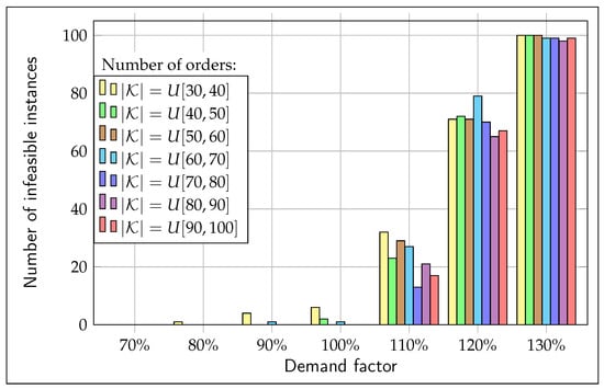
Figure 1.
Infeasible instances for each instance family.
Figure 2 and Figure 3 show scatter plots of runtimes for the instances grouped by instance family. Figure 2 presents runtimes grouped by the number of orders, allowing for an analysis of how solver performance varies with this factor. Figure 3 groups runtimes by the demand factor, offering a complementary perspective on its impact on runtimes.
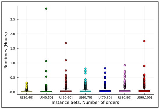
Figure 2.
Runtimes for optimal runs experiment grouped by number of orders, Experiment 1.
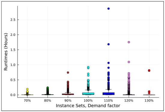
Figure 3.
Runtimes for optimal runs experiment grouped by demand factor, Experiment 1.
The R and metrics provide insights into runtime variability. The R metric exhibits high dispersion, indicating significant variation in runtimes across instances. However, the metric, which excludes outliers (with the count per instance family represented by ), offers a more robust measure of the runtime range. Moreover, this range tends to increase as the number of orders and/or the demand factor grows.
The metric is a more robust indicator of runtimes than , as it excludes outliers. The central tendency of runtimes increases as the number of orders and/or the demand factor grows. In Figure 2, after removing outliers, a slight upward trend is observed with increasing order numbers. Figure 3 shows a more pronounced upward trend as the demand factor increases. However, in this analysis, the instance family with a demand factor of 130% should be disregarded, as it includes only five instances.
The and metrics are influenced by the optimization solver used. These metrics provide valuable insights into the solver’s performance. Specifically, the metric indicates that the proportion of instances requiring execution times longer than 120 s increases as the number of orders and/or the demand factor grows. Additionally, the metric identified 41 instances that faced significant challenges in converging to the optimal solution, with their runtimes exceeding 1600 s.
Metrics and were used to select instances for conducting Experiments 2 and 3, which are discussed in the following sections.
Based on the evidence reported in Experiment 1, a clear relationship is observed between the demand factor and both the runtime duration and its dispersion. As the demand factor increases, not only do the runtimes tend to grow, but their variability also becomes more pronounced, even after removing outliers. This suggests that higher demand levels contribute to greater computational complexity. Additionally, feasibility becomes more challenging at elevated demand levels, as indicated by an increased number of instances requiring extended runtimes or failing to converge efficiently.
4.3. Experiment 2
The following definitions are introduced to present the results of Experiments 2 and 3. For a problem instance i, let denote the optimal solution and the solution found by the solver within a limited resolution time. The total costs of these solutions, represented as and , are calculated by summing Equations (1)–(4).
To analyze the solver’s performance, we present the results of the relative deviation while grouping instances by demand factor. The relative deviation between the solution and is defined as:
The number of analyzed instances for each demand factor family, based on the metric from Table 3, is as follows: For demand factors of 70%, 80%, 90%, 100%, 110%, 120%, and 130%, the respective instance counts are 16, 78, 188, 310, 309, 126, and 5. Note that represents the number of instances with a runtime exceeding 120 s.
The left-hand side of Figure 4, Figure 5, Figure 6, Figure 7 and Figure 8 displays histograms showing the relative deviation for each family of demand factors. Two important points regarding the histograms are: (i) The histogram of families with demand factors of 70% and 130% has been omitted due to insufficient sample size; (ii) For the demand factor families of 110% and 120%, the solver failed to find a solution within the 30-s time limit for three and four instances, respectively. Consequently, these instances have been excluded from the histograms.
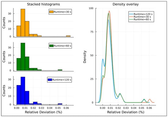
Figure 4.
Relative deviation distribution for instances with 80% demand factor, Experiment 2.
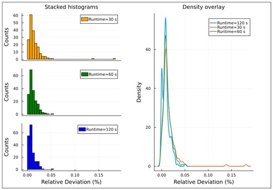
Figure 5.
Relative deviations distribution for instances with 90% demand factor, Experiment 2.
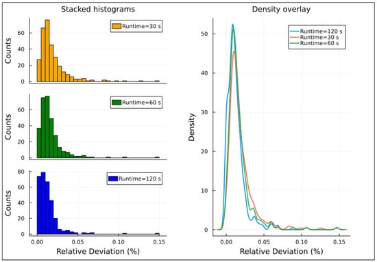
Figure 6.
Relative deviations distribution for instances with 100% demand factor, Experiment 2.
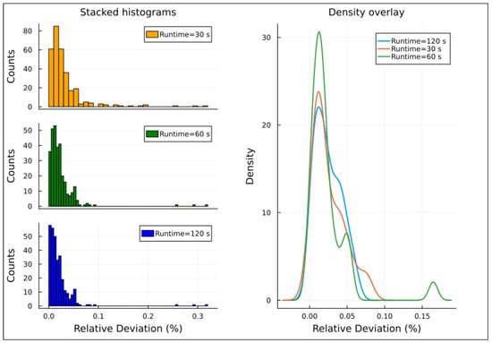
Figure 7.
Relative deviations distribution for instances with 110% demand factor, Experiment 2.
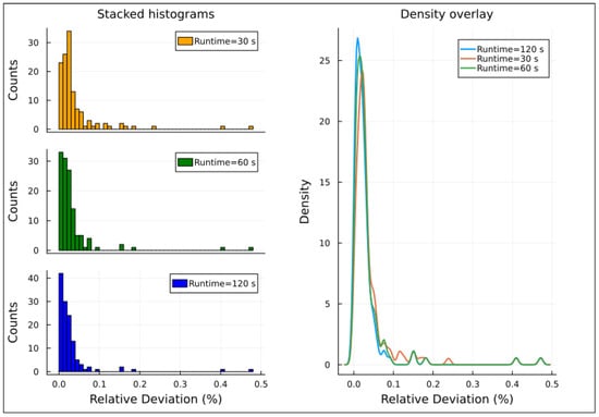
Figure 8.
Relative deviations distribution for instances with 120% demand factor, Experiment 2.
The right-hand side of Figure 4, Figure 5, Figure 6, Figure 7 and Figure 8 presents density overlay graphs illustrating the distribution of relative deviation for each resolution time (30, 60, and 120 s). In all these graphs, a decrease in relative deviation is evident as the resolution time increases. Specifically, as the resolution time lengthens, the density curve shifts to the left, indicating that solutions achieved over longer runtimes tend to be closer to the optimal solution. Furthermore, the area under the density curve becomes more concentrated around lower relative deviation values, suggesting that the solutions achieved are more accurate.
The seven instances excluded from the histograms because the solver did not provide a solution within 30 s exhibited no differences in their relative deviations when the resolution time was increased from 60 to 120 s. The relative deviations for these instances ranged from 0.0022% to 0.4715%.
Based on the evidence reported in Experiment 2, higher demand factors are associated with a greater number of instances requiring over 120 s to solve and with greater variability in solution quality under short time limits. When using the free solver HiGHS, longer resolution times consistently yield solutions closer to the optimum, with relative deviations decreasing as time increases.
4.4. Experiment 3
According to the metric reported in Table 3, 41 out of 4900 instances required more than 1600 s to reach an optimal solution. These instances, classified as hard instances, were solved within a time limit of 300 s.
On the left-hand side of Figure 9, histograms display the relative deviation for hard instances with resolution times of 30, 60, 120, and 300 s. On the right-hand side, a density overlay graph illustrates that, for these hard instances, increasing the runtime is beneficial for achieving higher-quality solutions. This highlights the trade-off between solution quality and the time taken to obtain them. As resolution time increases, the relative deviation decreases, with the density curve shifting to the left, indicating that longer runtimes yield solutions closer to the optimal.
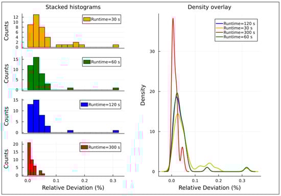
Figure 9.
Relative deviations distribution for hard instances, Experiment 3.
Figure 10 illustrates the mean, median, minimum, and maximum relative deviations concerning the runtime limit. For the hard instances, runs with a 300-s time limit achieve relative deviations ranging from 0.0005% to 0.0529%, with a mean of 0.0144%. The figure also indicates that the results from the 60 and 120 s runs are identical. Moreover, it highlights that the main advantage of using a 300 s time limit is the significant reduction in the observed worst-case performance, as indicated by the maximum value.
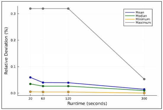
Figure 10.
Relative deviations versus runtimes for hard instances, Experiment 3.
Based on the evidence reported in Experiment 3, allowing a 300 s time limit when using the free optimization solver HiGHS leads to substantial improvements in solution quality for hard instances. This extended runtime significantly reduces relative deviations, especially in worst-case scenarios, and clearly proves beneficial compared to shorter limits of 30, 60, or 120 s.
4.5. Experiment 4
Table 4 summarizes the computational performance of the HiGHS and CPLEX solvers across the set of hard instances. For all instances, the runtime ratio (CPLEX/HiGHS) is significantly below 1, indicating that CPLEX consistently outperforms HiGHS in terms of resolution time. This result underscores a notable time-saving advantage when choosing the commercial solver.
Table 4.
Comparison of HiGHS and CPLEX optimal runtimes.
The “Runtime difference” column quantifies the time saved by opting for CPLEX over HiGHS for each instance. Although CPLEX is a commercial tool, these savings are especially relevant in time-sensitive applications or when solving large-scale instances that would otherwise require considerable computational effort with open-source alternatives.
The last row of Table 4 reports average values. On average, CPLEX solves hard instances in 195.93 s, while HiGHS requires 2645.94 s, resulting in an average runtime reduction of 2450.01 s. In relative terms, CPLEX uses only 8.02% of the time required by HiGHS, highlighting its strong advantage in computational efficiency.
The third instance in Table 4 clearly illustrates that convergence issues persist even when considering alternative solvers, reinforcing the inherent NP-hard nature of lot-sizing problems.
4.6. Experiment 5
According to the “CPLEX runtime” column in Table 4, five instances required more than 300 s for the solver to reach the optimal solution. Table 5 reports the total cost (objective function value) obtained by each solver for these instances under a 300-s time limit. Since both solvers reached the time limit without proving optimality, the reported solutions are approximate. The relative deviation between the solutions obtained by HiGHS and CPLEX is shown in the last column. On average, the commercial solver (CPLEX) produced solutions with a 0.0131% improvement in total cost compared to HiGHS, highlighting a small but consistent advantage even under strict runtime constraints.
Table 5.
Performance comparison on selected instances for 300-s time limit.
5. Discussion
The empirical evidence gathered from our experimentation provides several important insights into the performance of the proposed model and the challenges associated with production planning in the context of the studied case.
First, the complexity of the problem becomes evident, particularly through the convergence issues observed in several instances. These issues highlight the necessity for strategies that reduce or standardize resolution times for specific cases, ensuring reliable performance across various scenarios. The analysis of solver performance across different instance families indicates that as the number of orders and demand factors increases, the time required to reach an optimal solution also rises, accompanied by greater variability. This stresses the increasing computational complexity associated with larger or more complex instances.
A clear relationship exists between the demand factor and both runtime and its variability. As the demand factor increases, runtimes tend to rise, and their variability becomes more pronounced. This indicates that higher demand levels lead to greater computational effort and, in some cases, challenges in reaching feasible solutions. Notably, the number of instances requiring extended runtimes or failing to converge efficiently increases as demand rises, further emphasizing the computational challenges.
Regarding solution quality, we observed that the relative deviation decreased as the runtime increased, indicating that longer resolution times tend to improve solution quality by reducing the gap from optimal values. For example, for particularly difficult instances, a runtime of 30 s was insufficient to obtain feasible solutions, while longer runtimes of 60 or 120 s yielded no additional improvement.
A substantial improvement is observed in solution quality when the runtime limit is extended to 300 s with the HiGHS solver. This extended runtime leads to a significant reduction in relative deviations, particularly in worst-case scenarios, and provides a clear advantage over shorter time limits of 30, 60, or 120 s. The increased solution quality is particularly relevant for hard instances, demonstrating the necessity of allowing more time for complex cases. In the worst-case scenario, the relative deviation was only 0.0529%.
Although the commercial solver CPLEX demonstrated a clear advantage in computational efficiency, requiring only 8.02% of the time taken by HiGHS to reach optimality, the relative deviation between the solutions remained minimal. On average, CPLEX yielded solutions with a 0.0131% improvement in total cost compared to HiGHS, indicating a marginal but consistent advantage in solution quality, even under strict runtime constraints. These results suggest that while HiGHS is a highly capable and efficient open-source alternative, CPLEX offers a slight edge in both speed and precision, particularly relevant in time-sensitive or large-scale industrial applications.
Finally, the results are particularly relevant for the company under study, which operates near its production capacity with limited resources. The existing machine capacity and current strategies for increasing capacity are inadequate to meet the increased demand, reinforcing the need for efficient production planning models that can accommodate variability and optimize resource utilization.
6. Conclusions
The proposed model accurately represents the studied problem: a multi-period, multi-item, single-stage capacitated lot-sizing problem under a make-to-order production policy with parallel machines and machine eligibility constraints. The computational results from the case study confirm the viability of using an exact optimization approach. The model supports master production scheduling by determining product lot sizes across a finite planning horizon, ensuring that demand orders and resource constraints are satisfied while minimizing total costs. An additional advantage is disaggregation at the order level, which enhances decision-making by enabling more precise scheduling to ensure timely fulfillment and higher levels of customer satisfaction.
The performance evaluation reveals convergence challenges for certain instances, emphasizing the computational complexity of the problem. A runtime limit of 300 s is considered suitable, as it balances computational efficiency with the ability to achieve high-quality solutions, aligning well with the characteristics of the problem. This time limit approach proves especially effective for more difficult instances, where shorter time limits fail to yield feasible or competitive solutions.
Our results also validate the use of free software as a viable alternative for solving the proposed model. In particular, the combination of the Julia programming language, the JuMP modeling interface, and the HiGHS solver demonstrated robust performance and accessibility for tackling computationally intensive problems.
When comparing commercial and free solvers, the commercial solver CPLEX proved significantly more efficient in terms of runtime for achieving optimal solutions. Furthermore, under limited time conditions (300 s), CPLEX consistently delivered slightly better approximate solutions. Nevertheless, the relative deviations between the results obtained with HiGHS and CPLEX were minimal. These differences, however, become more pronounced as the problem complexity increases, as illustrated by experimentation. In summary, for limited runtimes and moderate-sized instances, both solvers provide satisfactory performance, making free solvers an attractive option when commercial licenses are unavailable. Beyond runtime and solution quality, other relevant performance aspects, such as memory usage, numerical stability, and scalability, may also play a role when comparing solver alternatives. Although these metrics were not addressed in the current study, they represent promising directions for future research aimed at enhancing our understanding of solver performance in large-scale or resource-constrained industrial contexts.
For future research, it would be beneficial to explore alternative mathematical formulations of the problem and evaluate their empirical behavior. A comparative analysis focusing on worst-case performance, particularly regarding relative deviations and resolution times, could further enhance understanding of model scalability and solver efficiency.
Author Contributions
Conceptualization, F.T.M. and J.U.-N.; methodology, F.T.M.; software, F.T.M.; validation, F.T.M. and J.U.-N.; formal analysis, F.T.M. and J.U.-N.; investigation, F.T.M. and J.U.-N.; data curation, J.U.-N.; writing—original draft preparation, F.T.M.; writing—review and editing, F.T.M. and J.U.-N.; visualization, F.T.M.; supervision, F.T.M.; project administration, F.T.M.; funding acquisition, F.T.M. All authors have read and agreed to the published version of the manuscript.
Funding
The APC for this article was funded by the Vice-Rectorate for Research and Graduate Studies and the Department of Industrial Engineering of the University of Bío-Bío.
Data Availability Statement
The implemented model and the instances used in this study are available at https://doi.org/10.5281/zenodo.15120475 (accessed on 1 April 2025), while the results are included within the article. The authors will make other files and source codes available upon request.
Conflicts of Interest
The authors declare no conflicts of interest.
References
- Guzman, E.; Andres, B.; Poler, R. Models and algorithms for production planning, scheduling and sequencing problems: A holistic framework and a systematic review. J. Ind. Inf. Integr. 2022, 27, 100287. [Google Scholar] [CrossRef]
- Wagner, S.; Sathe, M.; Schenk, O. Optimization for process plans in sheet metal forming. Int. J. Adv. Manuf. Technol. 2014, 71, 973–982. [Google Scholar] [CrossRef]
- Verlinden, B.; Cattrysse, D.; Crauwels, H.; Van Oudheusden, D. The development and application of an integrated production planning methodology for sheet metal working SMEs. Prod. Plan. Control 2009, 20, 649–663. [Google Scholar] [CrossRef]
- Askri, T.; Hajej, Z.; Rezg, N. Jointly production and correlated maintenance optimization for parallel leased machines. Appl. Sci. 2017, 7, 461. [Google Scholar] [CrossRef]
- Hajej, Z.; Rezg, N.; Askri, T. Joint optimization of capacity, production and maintenance planning of leased machines. J. Intell. Manuf. 2020, 31, 351–374. [Google Scholar] [CrossRef]
- Siemiatkowski, M.S.; Deja, M. Planning optimised multi-tasking operations under the capability for parallel machining. J. Manuf. Syst. 2021, 61, 632–645. [Google Scholar] [CrossRef]
- Wu, J.; Zhang, D.; Yang, Y.; Wang, G.; Su, L. Multi-stage multi-product production and inventory planning for cold rolling under random yield. Mathematics 2022, 10, 597. [Google Scholar] [CrossRef]
- Furtado, M.G.S.; Camargo, V.C.B.; Toledo, F.M.B. The production planning problem of orders in small foundries. Rairo-Oper. Res. 2019, 53, 1551–1561. [Google Scholar] [CrossRef]
- Zhang, Z.; Zhao, Z.; Qin, S.; Liu, S.; Zhou, M. Multi-product multi-stage multi-period resource allocation for minimizing batch-processing steel production cost. IEEE Trans. Autom. Sci. Eng. 2025, 22, 5272–5283. [Google Scholar] [CrossRef]
- Vanzetti, N.; Broz, D.; Corsano, G.; Montagna, J.M. An optimization approach for multiperiod production planning in a sawmill. For. Policy Econ. 2018, 97, 1–8. [Google Scholar] [CrossRef]
- Pastor, R.; Altimiras, J.; Mateo, M. Planning production using mathematical programming: The case of a woodturning company. Comput. Oper. Res. 2009, 36, 2173–2178. [Google Scholar] [CrossRef]
- Farrell, R.R.; Maness, T.C. A relational database approach to a linear programming-based decision support system for production planning in secondary wood product manufacturing. Decis. Support Syst. 2005, 40, 183–196. [Google Scholar] [CrossRef]
- Bayá, G.; Canale, E.; Nesmachnow, S.; Robledo, F.; Sartor, P. Production optimization in a grain facility through mixed-integer linear programming. Appl. Sci. 2022, 12, 8212. [Google Scholar] [CrossRef]
- Popović, D.; Bjelić, N.; Vidović, M.; Ratković, B. Solving a production lot-sizing and scheduling problem from an enhanced inventory management perspective. Mathematics 2023, 11, 2099. [Google Scholar] [CrossRef]
- Amorim, P.; Belo-Filho, M.A.F.; Toledo, F.M.B.; Almeder, C.; Almada-Lobo, B. Lot sizing versus batching in the production and distribution planning of perishable goods. Int. J. Prod. Econ. 2013, 146, 208–218. [Google Scholar] [CrossRef]
- Firat, M.; De Meyere, J.; Martagan, T.; Genga, L. Optimizing the workload of production units of a make-to-order manufacturing system. Comput. Oper. Res. 2022, 138, 105530. [Google Scholar] [CrossRef]
- Milne, R.J.; Wang, C.-T.; Denton, B.T.; Fordyce, K. Incorporating contractual arrangements in production planning. Comput. Oper. Res. 2015, 53, 353–363. [Google Scholar] [CrossRef]
- Bazargan-Lari, M.R.; Taghipour, S.; Zaretalab, A.; Sharifi, M. Planning and scheduling of a parallel-machine production system subject to disruptions and physical distancing. IMA J. Manag. Math. 2023, 34, 721–745. [Google Scholar] [CrossRef]
- Mula, J.; Díaz-Madroñero, M.; Andres, B.; Poler, R.; Sanchis, R. A capacitated lot-sizing model with sequence-dependent setups, parallel machines and bi-part injection moulding. Appl. Math. Model. 2021, 100, 805–820. [Google Scholar] [CrossRef]
- Cunha, A.L.; Santos, M.O. Mathematical modelling and solution approaches for production planning in a chemical industry. Pesqui. Oper. 2017, 37, 311–331. [Google Scholar] [CrossRef]
- Hsieh, S.; Chiang, C.-C. Manufacturing-to-sale planning model for fuel oil production. Int. J. Adv. Manuf. Technol. 2001, 18, 303–311. [Google Scholar] [CrossRef]
- Zhao, H.; Ierapetritou, M.G.; Rong, G. Production planning optimization of an ethylene plant considering process operation and energy utilization. Comput. Chem. Eng. 2016, 87, 1–12. [Google Scholar] [CrossRef]
- Campo, E.A.; Cano, J.A.; Gómez-Montoya, R.A. Linear programming for aggregate production planning in a textile company. Fibres Text. East. Eur. 2018, 26, 13–19. [Google Scholar] [CrossRef]
- Kalay, S.; Taşkın, Z.C. A Branch-and-Price algorithm for parallel machine campaign planning under sequence dependent family setups and co-production. Comput. Oper. Res. 2021, 135, 105430. [Google Scholar] [CrossRef]
- De Armas, J.; Laguna, M. Parallel machine, capacitated lot-sizing and scheduling for the pipe-insulation industry. Int. J. Prod. Res. 2019, 58, 800–817. [Google Scholar] [CrossRef]
- Tunca, O.; Erdal, F.; Sağsöz, A.E.; Çarbaş, S. Structural features of cold-formed steel profiles. Chall. J. Struct. Mech. 2018, 4, 77–81. [Google Scholar] [CrossRef]
- Veljkovic, M.; Johansson, B. Light steel framing for residential buildings. Thin-Walled Struct. 2006, 44, 1272–1279. [Google Scholar] [CrossRef]
- Vivan, A.L.; Paliari, J.C. Assembly line for the production of light gauge steel frame modular housing. Gest. Prod. 2021, 28, e5213. [Google Scholar] [CrossRef]
- Wang, B.; Gilbert, B.P.; Molinier, A.M.; Guan, H.; Teh, L.H. Shape optimisation of cold-formed steel columns with manufacturing constraints using the Hough transform. Thin-Walled Struct. 2016, 106, 75–92. [Google Scholar] [CrossRef]
- Yu, W.W.; LaBoube, R.A.; Chen, H. Cold-Formed Steel Design, 5th ed.; John Wiley & Sons: Hoboken, NJ, USA, 2019; ISBN 978-1-119-48741-8. [Google Scholar]
- Díaz-Madroñero, M.; Mula, J.; Peidro, D. A review of discrete-time optimization models for tactical production planning. Int. J. Prod. Res. 2014, 52, 5171–5205. [Google Scholar] [CrossRef]
- Pochet, Y.; Wolsey, L.A. Production Planning by Mixed Integer Programming; Springer: New York, NY, USA, 2006. [Google Scholar] [CrossRef]
- Luo, D.; Thevenin, S.; Dolgui, A. A state-of-the-art on production planning in Industry 4.0. Int. J. Prod. Res. 2022, 61, 6602–6632. [Google Scholar] [CrossRef]
- Cheraghalikhani, A.; Khoshalhan, F.; Mokhtari, H. Aggregate production planning: A literature review and future research directions. Int. J. Ind. Eng. Comput. 2019, 10, 309–330. [Google Scholar] [CrossRef]
- Demirel, E.; Özelkan, E.C.; Lim, C. Aggregate planning with flexibility requirements profile. Int. J. Prod. Econ. 2018, 202, 45–58. [Google Scholar] [CrossRef]
- Gansterer, M. Aggregate planning and forecasting in make-to-order production systems. Int. J. Prod. Econ. 2015, 170, 521–528. [Google Scholar] [CrossRef]
- Gao, Z.; Li, D.; Wang, D.; Yu, Z. Lagrange relaxation for the capacitated multi-item lot-sizing problem. Appl. Sci. 2024, 14, 6517. [Google Scholar] [CrossRef]
- Florian, M.; Lenstra, J.K.; Rinnooy Kan, A.H.G. Deterministic production planning: Algorithms and complexity. Manag. Sci. 1980, 26, 669–679. [Google Scholar] [CrossRef]
- Bitran, G.R.; Yanasse, H.H. Computational complexity of the capacitated lot size problem. Manag. Sci. 1982, 28, 1174–1186. [Google Scholar] [CrossRef]
- Buschkühl, L.; Sahling, F.; Helber, S.; Tempelmeier, H. Dynamic capacitated lot-sizing problems: A classification and review of solution approaches. OR Spectr. 2010, 32, 231–261. [Google Scholar] [CrossRef]
- Cardona-Valdés, Y.; Nucamendi-Guillén, S.; Peimbert-García, R.E.; Macedo-Barragán, G.; Díaz-Medina, E. A New formulation for the capacitated lot sizing problem with batch ordering allowing shortages. Mathematics 2020, 8, 878. [Google Scholar] [CrossRef]
- Rehman, H.U.; Ahmad, A.; Ali, Z.; Baig, S.A.; Manzoor, U. Optimization of aggregate production planning problems with and without productivity loss using Python PuLP package. Manag. Prod. Eng. Rev. 2021, 12, 38–44. [Google Scholar] [CrossRef]
- Zhang, R.; Zhang, L.; Xiao, Y.; Kaku, I. The activity-based aggregate production planning with capacity expansion in manufacturing systems. Comput. Ind. Eng. 2012, 62, 491–503. [Google Scholar] [CrossRef]
- Lee, C.-W.; Doh, H.-H.; Lee, D.-H. Capacity and production planning for a hybrid system with manufacturing and remanufacturing facilities. Proc. Inst. Mech. Eng. Part B-J. Eng. Manuf. 2015, 229, 1645–1653. [Google Scholar] [CrossRef]
- Fiorotto, D.J.; De Araujo, S.A.; Jans, R. Hybrid methods for lot sizing on parallel machines. Comput. Oper. Res. 2015, 63, 136–148. [Google Scholar] [CrossRef]
- Tempelmeier, H.; Copil, K. Capacitated lot sizing with parallel machines, sequence-dependent setups, and a common setup operator. OR Spectr. 2016, 38, 819–847. [Google Scholar] [CrossRef]
- Wu, T.; Xiao, F.; Zhang, C.; He, Y.; Liang, Z. The green capacitated multi-item lot sizing problem with parallel machines. Comput. Oper. Res. 2018, 98, 149–164. [Google Scholar] [CrossRef]
- Absi, N.; Kedad-Sidhoum, S. MIP-based heuristics for multi-item capacitated lot-sizing problem with setup times and shortage costs. Rairo-Oper. Res. 2007, 41, 171–192. [Google Scholar] [CrossRef]
- Kim, T.; Glock, C.H. Production planning for a two-stage production system with multiple parallel machines and variable production rates. Int. J. Prod. Econ. 2018, 196, 284–292. [Google Scholar] [CrossRef]
- Absi, N.; Kedad-Sidhoum, S. The multi-item capacitated lot-sizing problem with safety stocks and demand shortage costs. Comput. Oper. Res. 2009, 36, 2926–2936. [Google Scholar] [CrossRef]
- Dunning, I.; Huchette, J.; Lubin, M. JuMP: A modeling language for mathematical optimization. SIAM Rev. 2017, 59, 295–320. [Google Scholar] [CrossRef]
- Lubin, M.; Dunning, I. Computing in operations research using Julia. INFORMS J. Comput. 2015, 27, 238–248. [Google Scholar] [CrossRef]
- Lubin, M.; Dowson, O.; Garcia, J.D.; Huchette, J.; Legat, B.; Vielma, J.P. JuMP 1.0: Recent improvements to a modeling language for mathematical optimization. Math. Prog. Comp. 2023, 15, 581–589. [Google Scholar] [CrossRef]
- Huangfu, Q.; Hall, J.A.J. Parallelizing the dual revised simplex method. Math. Prog. Comp. 2018, 10, 119–142. [Google Scholar] [CrossRef]
- Bezanson, J.; Edelman, A.; Karpinski, S.; Shah, V.B. Julia: A fresh approach to numerical computing. SIAM Rev. 2017, 59, 65–98. [Google Scholar] [CrossRef]
- The Julia Programming Language. Available online: https://julialang.org (accessed on 3 October 2024).
- JuMP. Available online: https://jump.dev/JuMP.jl/stable (accessed on 3 October 2024).
- HiGHS—High Performance Software for Linear Optimization. Available online: https://highs.dev (accessed on 3 October 2024).
- IJulia.jl. Available online: https://github.com/JuliaLang/IJulia.jl (accessed on 17 March 2025).
- Jupyter. Available online: https://jupyter.org/ (accessed on 17 March 2025).
- HiGHS.jl. Available online: https://github.com/jump-dev/HiGHS.jl (accessed on 17 March 2025).
- HiGHS Documentation—High Performance Optimization Software. Available online: https://ergo-code.github.io/HiGHS/dev (accessed on 17 March 2025).
- HiGHS Documentation—Solvers. Available online: https://ergo-code.github.io/HiGHS/dev/solvers/#solvers (accessed on 17 March 2025).
- CPLEX.jl. Available online: https://github.com/jump-dev/CPLEX.jl (accessed on 1 May 2025).
- XLSX.jl. Available online: https://juliapackages.com/p/xlsx (accessed on 17 March 2025).
- Muñoz, F.T. Experimental Data for “A Make-to-Order Capacitated Lot-Sizing Model with Parallel Machines, Eligibility Constraints, Extra Shifts, and Backorders” [Data Set]. 2025. Available online: https://doi.org/10.5281/zenodo.15120475 (accessed on 27 May 2025).
- Biblioteca del Congreso Nacional de Chile—BCN. Establishes the Consolidated, Coordinated and Systematized Text of the Labor Code. Available online: https://bcn.cl/2erv4 (accessed on 3 October 2024).
- Ulloa, J.G. Propuesta de un Modelo de Optimización para Mejorar el Proceso de Planificación de la Producción en la Familia de Productos Metalcon. Bachelor’s Thesis, Universidad del Bío-Bío, Concepción, Chile, 8 April 2022. [Google Scholar]
Disclaimer/Publisher’s Note: The statements, opinions and data contained in all publications are solely those of the individual author(s) and contributor(s) and not of MDPI and/or the editor(s). MDPI and/or the editor(s) disclaim responsibility for any injury to people or property resulting from any ideas, methods, instructions or products referred to in the content. |
© 2025 by the authors. Licensee MDPI, Basel, Switzerland. This article is an open access article distributed under the terms and conditions of the Creative Commons Attribution (CC BY) license (https://creativecommons.org/licenses/by/4.0/).