Abstract
This paper is devoted to the experimental study of the integral approximation method in entropy optimization problems arising from the application of the Randomized Machine Learning method. Entropy-optimal probability density functions contain normalizing integrals from multivariate exponential functions; as a result, when computing these distributions in the process of solving an optimization problem, it is necessary to ensure efficient computation of these integrals. We investigate an approach based on the approximation of integrand functions, which are applied to the solution of several configurations of problems with model and real data with linear static models using a symbolic computation mechanism. Computational studies were carried out under the same conditions, with the same initial data and values of hyperparameters of the used models. They have shown the performance and efficiency of the proposed approach in the Randomized Machine Learning problems based on linear static models.
Keywords:
randomized machine learning; entropy; optimization; symbolic computations; symbolic integration; numerical methods MSC:
62F35; 41A10; 68W20; 68W30
1. Introduction
Randomized Machine Learning is a new scientific area based on the concept of artificial randomization of model parameters. This approach transforms a traditional model with fixed parameters into a model with random parameters. Instead of searching for specific parameter values, the model learns to find their probability distributions during training. These distributions are chosen to maximize their entropy while maintaining the moments of the model output.
One of the key advantages of this method is its independence from the real properties of the input data. This method does not require testing hypotheses about the normality of the data or studying other statistical characteristics of the data. The distributions obtained as a result of training are determined by the conditions of maximum entropy, which corresponds to the most unfavorable scenario of the investigated process characterized by the maximum degree of uncertainty. These properties of the entropy estimation method date back to the works of Boltzmann [1], Jaynes [2,3], Shannon [4]. A significant contribution to the further development of this concept was made by the studies of Kapur [5], Golan [6,7] and a number of other researchers.
An important feature of the method is the ability to simultaneously find entropy-optimal distributions of noise components together with optimal distributions of model parameters. This distinguishes this method from traditional approaches, where we have to make assumptions about the characteristics of the noise and the data.
The main theoretical foundations of the method are presented in [8], and by now, sufficient experience has been accumulated in its successful application to various forecasting problems, classification, missing data recovery, and a number of other problems. Nevertheless, the experience of its practical application has shown some of its properties that require further research. One of such properties is the necessity to compute multivariate integrals in the process of solving the main optimization problem of Machine Learning, which in practice is solved by the iterative numerical method. Numerical integration in most software frameworks is performed by methods based on quadrature formulas, effective software implementations of which are developed for dimensionalities not higher than three. In order to solve the described problem, it was proposed to use the approximation of exponents in integrand functions by Taylor (Maclaurin) series.
Thus, the present work is aimed at further development of the Randomized Machine Learning (RML) method in the direction of developing effective approaches to the implementation of their computational component, in particular, an experimental study of their practical implementation and effectiveness using synthetic and real data.
2. Problem Statement
The application of the methodology of Randomized Machine Learning leads to the problem of optimizing the information entropy of the distributions of parameters and noise of the trained model.
Within the framework of this methodology, we consider models in the “input-output” form, in which the transformation of input into output is realized in the general case by a nonlinear function or functional.
It follows from such a general description that the transformation of input to output can be realized by both numerical and functional objects. In particular, one can consider a model as taking a continuous function as input and giving a function as output as well.
On the other hand, in the context of the study of processes functioning in time (often understood in a generalized sense), a productive approach is the approach related to the observation of the state of the process, which occurs at some time intervals, thus forming a set of state observations. It is important here that the observations do not occur continuously, and thus there is a countable set of observation points.
A natural way to describe the transformation of input into output is its functional parameterized description. The parameters of such a transformation are proposed to be tuned (trained) by the data at the observation points, which are “real data” in this procedure.
The transformation of input into output, and, accordingly, the model, will be called static only if its previous state is needed to form the output, i.e., the next state, of the model. In case its previous states, in particular p of previous states, are necessary, then dynamic coupling is realized.
In this paper, we consider linear static models. Despite their simplicity, they are used in most statistical methods as well as within such scientific and applied areas as Data Mining, Machine Learning, and Artificial Intelligence due to their structural simplicity, interpretability, and availability of a large number of methods for working with them.
Consider a model with n inputs and one output y, the transformation between which is realized by the function , where is the vector of model inputs and is the vector of parameters. The parameters are assumed to be random and of interval type with joint probability distribution
In this paper, we consider the linear models, and hence the function z can be represented in the form of a generalized dot product
It is assumed that the state of the process under study contains errors that determine its stochastic component. This randomness is taken into account in modeling by means of additive noise at the model output, which also has an interval type with the distribution
Randomized Machine Learning is based on the idea of estimating model parameters simultaneously with measurement noise under the assumption that the parameters of the model under study are random, and their estimates resulting from the method are not their values or intervals but their probability distributions. This goal is achieved by solving the problem of maximizing the entropy of the distributions of the model parameters under conditions of balance at the moments of the model output with the observed real data
Entropy-optimal distributions (their probability density functions) of parameters and noises, depending on Lagrange multipliers, are given by the following expressions:
where —vector of Lagrange multipliers.
To determine the Lagrange multipliers, it is necessary to solve the following equation:
Despite the fact that the system (6) is solved numerically, any numerical methods for solving such problems have an iterative character where, at each iteration, it is required to calculate the value of the left-hand side of the equation for the current value of the optimized variable. In the case of the system under consideration, this operation is significantly complicated due to the presence of integral components.
Numerical computation of multivariate integrals is a challenging problem in general, which is relatively efficiently solved on most computing platforms using quadrature methods for dimensionalities of three or less. For higher dimensionality, it is necessary to involve Monte Carlo methods, the accuracy of which is inversely proportional to the square root of the number of trials (random grid points), which is further aggravated by the higher dimensionality, requiring an increase in the number of points to achieve the required accuracy.
In order to solve the described problem in [9], it was proposed to use the approximation of exponents by Taylor (Maclaurin) series, which is possible due to the analyticity of the exponent, in particular, the exponents under the integrals in the expressions (5) and (6) will be approximated by Maclaurin series for the exponent from the scalar variable f with a finite number of terms. In the framework of this paper, we study the case with four terms of the series
We believe that the choice of four terms of Taylor series is optimal in terms of accuracy and computational performance at the current stage of this study.
3. Materials and Methods
The purpose of this paper is to experimentally investigate the practical feasibility and efficiency of the proposed approach based on the application of the RML method to various linear models with three numerical implementation variants: fully numerical, hereafter denoted as numeric or num, exact (exact or exp), based on the exact calculation of exponents, and approximate (approximate or app).
The first variant realizes the numerical computation of the corresponding integrals using methods based on quadrature formulas, respectively, and its application is possible for parameter dimensionalities not higher than 3.
The second and third variants are based on the direct computation of the integrals included in the corresponding expressions. This approach is based on the use of the symbolic computation mechanism implemented in many software platforms, such as MATLAB and Python. This mechanism allows expressions to be formed and manipulated in a manner similar to that of a human. Of course, its functionality has certain limitations that lead to the practical impossibility of manipulating bulky expressions due to the lack of computational resources, such as memory. In this regard, it is particularly relevant to verify the realizability of this approach to the studied problem.
In view of the above, under the exact (but still numerical) solution, we mean the computation of the corresponding integrals using symbolic computations, and a similar principle is applied to the approximate solution, where the corresponding expressions of integrand functions implement the Taylor series expansion with a given number of terms.
The study of this approach will be carried out on two groups of models with corresponding data. The first group represents artificially created data generated by the model with specified characteristics, as a consequence of which a variety of concrete data realizations are achieved. The second group represents real data related to the task of forecasting the area of thermokarst lakes, which are characterized by the fact that their probabilistic characteristics are unknown. In all cases, the data are scaled to the interval to avoid error accumulation and overflow in the computations.
The purpose of the ongoing experimental study is to establish the closeness of the obtained solutions in Equation (6), as well as the closeness of the obtained entropy-optimal distributions (4) and (5).
3.1. Model Data
The model data to be used in the following are generated by a linear static model of order p of the form
where y—model output, —input, —random noise of standard normal distribution, n—time index, —parameters.
Under the assumption that the model realizes some process, observations of its development at some time points n give a set of real data that will be used to train the model. For the purposes of this study, in accordance with the model, we generate different data for any value of the vector parameter and different values of the model order p and the number of observation points N, and the inputs are generated randomly with a uniform distribution from the interval .
Since the purpose of this paper is to investigate the realizability of the proposed method for a different number of data points and dimensionalities of the integration space, we further use the notation D for the dimensionality of the parameter vector (in the context of the model (7) ), and the reference to the corresponding data configuration is dDnN.
We generate the data for the study for and . Examples of some generated data configurations are shown in Figure 1, Figure 2 and Figure 3, where the graphs labeled real show the generated data and the graphs labeled model show the model trajectory obtained by the least squares for the model used.
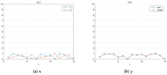
Figure 1.
Model data d2n15.
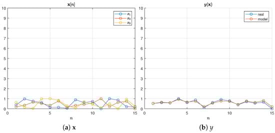
Figure 2.
Model data d3n15.
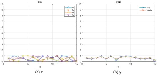
Figure 3.
Model data d4n15.
3.2. Real Data
As a model of the real process and the data corresponding to it, we consider the model of the thermokarst lakes area in Western Siberia, considered in a number of publications [10,11,12] devoted to the study of this object, the importance and relevance of the study of which is ensured by the fact that thermokarst lakes are a massive source of greenhouse gases. In the present work, this object and related data are interesting and chosen by us for the reasons that, despite the structural simplicity of the model used, the data on which it is necessary to train it are characterized by two main circumstances: their small amount and large errors of unknown nature in the probabilistic sense. These circumstances are related to the fact that some data are collected from only a few points in vast, inaccessible areas, and others are obtained by methods of analyzing low-resolution satellite images, resulting in a small amount of noisy data.
The model to be considered here is a linear static model with two inputs, which establishes the relationship between area S and two natural factors: precipitation R and temperature T, whose data are annually averaged. We use two types of it: with a free parameter or without, in order to use the same data, namely
Similar to the model data, we consider three data configurations, lakes_d2n5, lakes_d2n10, and lakes_d3n5, obtained by selecting the appropriate number of consecutive points from the available dataset. The real data for the two configurations are shown in Table 1 and Figure 4 and Figure 5, where R is scaled to .

Table 1.
Data for the thermokarst lake area model.
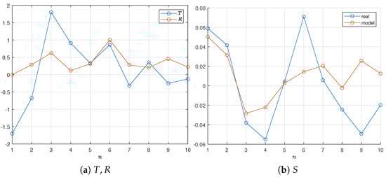
Figure 4.
Data lakes_d2n10.
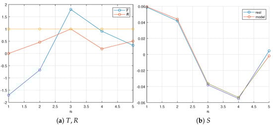
Figure 5.
Data lakes_d3n5.
3.3. Entropy Maximization Procedure
The use of symbolic calculation mechanisms in practice involves the necessity of separating work with numeric and symbolic objects within a single program code. Otherwise, there may be problems with the accuracy of calculations and/or their speed [13]. In most implementations of symbolic computations, it is recommended to convert all numeric values that are included in symbolic expressions into a symbolic representation, or to substitute them instead of the corresponding symbols at the final stage of computation, when the numeric result of some expression is required.
The problems considered in this paper are characterized by the fact that the integrand functions include the values of inputs at the observation points , as well as Lagrange multipliers , and integration is required to be performed over the parameters . It should be taken into account that the solution of the problem (6) is performed by an iterative numerical optimization method, which leads to the need to calculate integrals for each new value of the optimized variable, i.e., .
Taking these circumstances into account, before starting the optimization, it is necessary to form symbolic expressions for the corresponding parts of the function to be optimized, namely for the integrals in the expression (6). In this case, to reduce the amount of symbolic calculations, these expressions are formed in several steps:
- The symbolic vectors for the variables , and the matrix of inputs , are formed;
- All values of the inputs are converted to symbolic form, and a set (vector) of symbolic representations of the function defined by (2) is formed;
- Compute the symbolic representation of the dot product function ;
- Now, we can compute two symbolic representations at once: one for the exact solution and another for the approximate solution by substituting the expression from the previous paragraph into the corresponding symbolic expression.The symbolic expression of the integrand function of the form is calculated in the same way.
This procedure allows us to obtain the expressions of the required integrand functions depending only on , thus performing cumbersome and relatively resource-intensive symbolic calculations once before starting the numerical solution of Equation (6). Inside the optimized function, the current values of are substituted into the corresponding symbolic expressions, and then the values of integrals are calculated, which are no longer resource-intensive.
3.4. Comparison
We propose to evaluate the feasibility and efficiency of our approach, taking into account its application to RML problems, by comparing the resulting Lagrange multipliers , as well as the resulting entropy-optimal parameter distributions (their probability density functions).
We compare the Lagrange multipliers obtained as a result of solving the corresponding problems for different configurations by two metrics: absolute and relative error in the norm:
where the relative error is calculated relative to the exact value.
It should be noted that in the case of comparison of multipliers, there are no serious problems, because here it is necessary to compare vectors according to the chosen metric. In the case of comparing distributions, however, certain difficulties may arise due to their dimensionality. Here, we propose to estimate the difference of distributions pointwise by calculating the mean square error (MSE) or mean absolute relative error (MAPE):
where value is “exact”, p—“model”, and N—number of points.
4. Results and Discussion
The implementation of all computational experiments was carried out in MATLAB version 9.7 (2019b) on Windows x64 platform equipped with Intel 3.00 GHz 8-core i7-9700F CPU and 32 GB of RAM. The Trust-Region-Dogleg [14] algorithm implemented in the Optimization Toolbox [15] was used to solve the system of Equation (6) with default options and initial , and symbolic calculations were implemented using the Symbolic Math Toolbox [13].
The Randomized Machine Learning problem was solved in all experiments for , , and the initial value of the corresponding optimization problems was .
4.1. Model Data
The obtained values of Lagrange multipliers for different configurations are contained in Table 2, Table 3 and Table 4, and the values of metrics are in Table 5.
Table 2.
Lagrange multipliers for .
Table 3.
Lagrange multipliers for .
Table 4.
Lagrange multipliers for .
Table 5.
Lagrange multipliers errors.
From the given data, we can see that for each value of dimension D in all three variants of the problem solution, numerical, exact, and approximate, the Lagrange multipliers obtained as a result of numerical optimization of the corresponding Equation (6) are close. This is evidenced by the values of absolute and relative errors, the latter of which do not exceed 5%.
We also observe the deviation of the solution obtained in the approximate version from the exact one, as well as from the numerical one, and the latter two are closer to each other. This situation is quite expected and is explained by the approximation using a Taylor series with only four terms. Increasing the terms of the series will predictably lead to an increase in accuracy, i.e., to an approximation to the exact solution by the metric used, but will significantly increase the load on computational resources and performance.
As for the dependence of the accuracy of the obtained solutions (in the sense of the used metric) on the dimensionality and the number of observation points, the obtained data did not reveal any significant dependence between these parameters. The order of the obtained errors keeps its stability in all variants of data configurations.
Let us now turn to the analysis of the obtained entropy-optimal distributions, which are the goal of RML. Figure 6 shows the bivariate distributions obtained in the configuration d2n10, and Table 6 shows the error values between the corresponding distributions for all investigated configurations.

Figure 6.
Entropy-optimal distributions for d2n10.
Table 6.
Distribution errors.
The given graphs show the structural closeness of the distributions (PDF functions) in the exact and approximate cases, and the values of the errors between all three variants of the solution allow us to state that this closeness is observed for the numerical solution as well.
It should be noted that unlike the solutions to the optimization problem, the errors between the distributions indicate some dependence on the dimensionality or the number of observation points—some increase in the relative error with increasing number of observation points is noticeable for all the dimensions investigated, and an increase in the error with increasing dimensionality for the same number of observation points can also be observed. All this can be explained by the fact that both the number of observation points and the dimensionality determine the value of the integrand function in the corresponding expressions, and, as a consequence, the integral from it. Due to the approximation of the integrand, the error increases, especially when the dimensionality increases.
Nevertheless, the obtained data show a relatively low level of error, which is acceptable for the problems on which the RML method is oriented, namely for problems with a small amount of noisy data.
4.2. Real Data
The obtained values of Lagrange multipliers for the real data configurations are contained in Table 7 and Table 8, the values of metrics are in Table 9, Figure 7 presents the entropy-optimal distributions obtained in the lakes_d2n10 configuration, and Table 10 summarizes the error values between the corresponding distributions.
Table 7.
Lagrange multipliers for .
Table 8.
Lagrange multipliers for .
Table 9.
Lagrange multipliers errors.
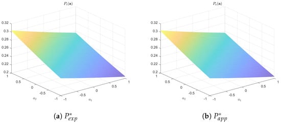
Figure 7.
Entropy-optimal distributions for lakes_d2n10.
Table 10.
Distribution errors.
In general, in the case of real data, for which, unlike artificial data, their probabilistic characteristics are unknown, we can draw the same conclusions, namely, low errors both in solving the optimization problem and between the obtained distributions.
4.3. Performance
The performance of the used algorithms was evaluated when solving problems on model data. Table 11 shows the solution time of the optimization problem, including the computation of the corresponding integrals. The columns time_* show the time of the solution of the problem, and the next three columns show the change in the time of realization of the corresponding solution compared with numerical (columns % exp and % app) and approximate compared with exact.
Table 11.
Performance indicators, seconds.
In general, the obtained performance results show the expected speedup of the solution in the case of using symbolic computations, since such computation allows us to compute their symbolic expression depending on once before starting the optimization, while a fully numerical solution requires the computation of the values of integrals for each value of , i.e., at each iteration, which significantly increases the amount of computation.
The computation of the approximate solution is expectedly slower than for the exact solution, which is due to the structurally more complex expressions, which are the sum of several terms of the series that need to be raised in degree. Although the arguments of these expressions are simple sums, the expressions themselves contain a much larger number of terms and multipliers, resulting in the need to build and manipulate large special data structures in memory. As a result, this leads to an increase in the time required to obtain a solution.
It should also be noted that some time indices for approximate variants differ from those for exact variants. This is due to the properties of the software platform used and the time required to build the corresponding program objects in memory. Such a process, called “warming up”, is standard for many program systems, including those using some type of parallelism.
5. Conclusions
The aim of this work was to experimentally investigate the approach to the efficient computation of integral components in problems arising in the application of the Randomized Machine Learning method. Entropy-optimal distributions (their probability densities) contain normalizing integrals from multivariate exponential functions; as a result, when computing these distributions in the process of solving an optimization problem, it is necessary to ensure efficient computation of these integrals. We investigated an approach based on the approximation of integrand functions by a Taylor series with four terms. The research methodology involved solving several problems with appropriate data configurations in two groups based on modeled, artificially generated data and real data. The workability and efficiency of the proposed approach were evaluated by the accuracy (closeness) of the solutions of the optimization problem for Lagrange multipliers, as well as by the closeness of the obtained entropy-optimal distributions. Computational studies were carried out under identical conditions, with the same initial conditions and values of hyperparameters of the models. They showed the workability and efficiency of our proposed approach in problems based on linear static models.
Author Contributions
Conceptualization, Y.S.P., A.Y.P., and Y.A.D.; data curation, Y.A.D. and I.V.S.; methodology, Y.S.P., A.Y.P., and Y.A.D.; software, A.Y.P., Y.A.D., and I.V.S.; supervision, Y.S.P.; writing—original draft, A.Y.P. and Y.A.D. All authors have read and agreed to the published version of the manuscript.
Funding
This research received no external funding.
Data Availability Statement
The original contributions presented in this study are included in the article. Further inquiries can be directed to the corresponding author.
Acknowledgments
The reported study was performed in the Research Laboratory of Young Scientists “Technologies for Analysis and Controllable Text Generation”.
Conflicts of Interest
The authors declare no conflicts of interest.
References
- Boltzmann, L. On connection between the second law of mechanical theory of heat and probability theory in heat equilibrium theorems. In Boltzmann L.E. Selected Proceedings; Shlak, L.S., Ed.; Classics of Science, Nauka: Moscow, Russia, 1984. [Google Scholar]
- Jaynes, E.T. Information theory and statistical mechanics. Phys. Rev. 1957, 106, 620–630. [Google Scholar] [CrossRef]
- Jaynes, E.T. Probability Theory: The Logic of Science; Cambridge University Press: Cambridge, UK, 2003. [Google Scholar]
- Shannon, C.E. Communication theory of secrecy systems. Bell Labs Tech. J. 1949, 28, 656–715. [Google Scholar] [CrossRef]
- Kapur, J.N. Maximum-Entropy Models in Science and Engineering; John Wiley & Sons: Hoboken, NJ, USA, 1989. [Google Scholar]
- Golan, A.; Judge, G.; Miller, D. Maximum Entropy Econometrics: Robust Estimation with Limited Data; John Wiley & Sons: New York, NY, USA, 1996. [Google Scholar]
- Golan, A. Foundations of Info-Metrics: Modeling, Inference, and Imperfect Information; Oxford University Press: Oxford, UK, 2018. [Google Scholar]
- Popkov, Y.S.; Popkov, A.Y.; Dubnov, Y.A. Entropy Randomization in Machine Learning; Chapman and Hall/CRC: New York, NY, USA, 2023. [Google Scholar] [CrossRef]
- Popkov, Y.S. Analytic method for solving one class of nonlinear equations. Dokl. Math. 2024, 110, 404–407. [Google Scholar] [CrossRef]
- Polischuk, V.Y.; Muratov, I.N.; Polischuk, Y.M. Problemi modelirovania prostranstvennoy strukturi polei termokarsovykh ozer v zone vechnoy merzloty na osnove sputnikovykh snimkov. Vestnik Yugorskogo Gosudarstvennogo Universiteta 2018, 88–100. [Google Scholar]
- Polischuk, V.Y.; Muratov, I.N.; Kuprianov, M.A.; Polischuk, Y.M. Modelirovanie polei termokarsovykh ozer v zone vechnoy merzloty na osnove geoimitacionnogo podhoda i sputnikovykh snimkov. Mat. Zametki SVFU 2020, 27, 101–114. [Google Scholar]
- Polischuk, V.Y.; Kuprianov, M.A.; Polischuk, Y.M. Analiz vzaimosvyazi izmeneniy klimata i dinamiki termokarsovykh ozer v arkticheskoy zone Taymyra. Sovrem. Probl. Distancionnogo Zondirovania Zemli Kosmosa 2021, 16. [Google Scholar]
- The MathWorks Inc. Symbolic Math Toolbox, version 9.4 (R2022b); The MathWorks Inc.: Natick, MA, USA, 2022. [Google Scholar]
- Nocedal, J.; Wright, S. Numerical Optimization; Springer Science & Business Media: Berlin/Heidelberg, Germany, 2006. [Google Scholar]
- The MathWorks Inc. Optimization Toolbox, version 9.4 (R2022b); The MathWorks Inc.: Natick, MA, USA, 2022. [Google Scholar]
Disclaimer/Publisher’s Note: The statements, opinions and data contained in all publications are solely those of the individual author(s) and contributor(s) and not of MDPI and/or the editor(s). MDPI and/or the editor(s) disclaim responsibility for any injury to people or property resulting from any ideas, methods, instructions or products referred to in the content. |
© 2025 by the authors. Licensee MDPI, Basel, Switzerland. This article is an open access article distributed under the terms and conditions of the Creative Commons Attribution (CC BY) license (https://creativecommons.org/licenses/by/4.0/).