A Finite-Time Disturbance Observer-Based Control for Constrained Second-Order Dynamical Systems and Its Application to the Attitude Tracking of a UAV

Abstract

As second-order dynamical systems are omnipresent, solving the control problem for such a class of systems has attracted worldwide attention. Among many techniques, the backstepping control method is well-known for its straightforward design and efficacy, yet it suffers from the inherent issue of complexity explosion. This work aims to leverage the backstepping method in a finite-time-converging control scheme. First, to address the presence of external disturbances, a nonlinear, unknown-input observer is introduced, which provides a disturbance estimate with finite-time convergence. Second, a fast-converging finite-time filter is used to estimate the derivative of virtual control inputs in the backstepping framework. Next, the outputs of the disturbance observer and the filter are used to formulate a finite-time, backstepping control law. Additionally, the closed-loop system is proven to be finite-time stable through a rigorous stability analysis. Finally, the proposed algorithm is applied to an unmanned aerial vehicle (UAV) system and validated through simulations and experiments under actual flight conditions. The experimental results demonstrate the feasibility of the implementation and the practical efficacy of the proposed approach.

1. Introduction

Second-order dynamical systems are prevalent in mechanical engineering applications and present various control challenges [1,2]. These systems often exhibit oscillatory dynamics due to inherent inertia and elasticity. Their response is even more complicated under the impacts of internal uncertainties and external disturbances [3]. Therefore, maintaining robust closed-loop stability has remained a primary concern. Equally important is achieving rapid and precise tracking performance, so that the system can accurately follow desired trajectories. Addressing these control problems is crucial to ensure that mechanical systems operate safely and meet prescribed performance requirements.

In the control of second-order dynamical systems, several nonlinear control techniques have been extensively studied and applied, including sliding mode control (SMC), nonlinear model predictive control (NMPC), fuzzy logic control (FLC), neural network-based control (NNBC), and backstepping control, just to name a few. The SMC is renowned for its robustness against system uncertainties and external disturbances [4,5]. Recent advancements have focused on mitigating the chattering phenomenon inherent in SMC by integrating it with other control strategies, such as backstepping and terminal sliding modes [6], to enhance performance and reduce steady-state errors. The NMPC is another prominent technique that utilizes system models to predict future behavior and optimize control inputs over a finite horizon [7], effectively handling multivariable systems with constraints. The FLC and NNBC have also gained attention [8], especially in scenarios with high uncertainty and nonlinearity, by leveraging their approximation capabilities and adaptability. Each of these techniques has its own advantages and shortcomings, which determine their suitability in specific applications.

Among such various control methods, the backstepping remains a go-to nonlinear control technique for second-order mechanical systems because it combines rigorous theoretical guarantees with practical design simplicity [9]. Its scheme breaks a nonlinear system into a hierarchy of lower-order subsystems (e.g., treating the angular rate as a virtual control for the angle) and designs stabilizing control laws for each subsystem [10,11]. This step-by-step construction of Lyapunov functions ensures the asymptotic stability of the overall closed-loop system by design [3]. Importantly, backstepping offers a high degree of flexibility: unlike exact feedback linearization, it does not demand canceling every nonlinearity with a perfect model but instead accommodates model dynamics through successive Lyapunov-guided adjustments. This makes it well suited to the typical Euler–Lagrange structure of mechanical systems [12] and the cascaded attitude–position loops of UAVs, which naturally have second-order dynamics.

In fact, backstepping is one of the most widely used nonlinear control methods for unmanned aerial vehicles [13,14], valued for its ability to ensure stable flight and improved control performance under nonlinear and coupled dynamics [10]. On the practical side, the methodology’s structured nature yields explicit control laws that are relatively straightforward to implement and tune. Backstepping controllers can thus be deployed on real mechanical devices or UAVs with relative ease, while leveraging adaptive or robust add-ons (neural networks, disturbance observers, etc.) [15] to handle uncertainties without losing the stability proofs. These combined strengths explain why backstepping continues to be extensively applied in controlling mechanical systems and UAVs in recent research [16].

Achieving finite-time convergence in backstepping control is of critical importance in applications involving mechanical systems [17] and unmanned aerial vehicles (UAVs), where the system states are required to reach the desired equilibrium within a bounded time interval, regardless of initial conditions [17]. This property is particularly advantageous in time-sensitive missions, such as obstacle avoidance, aggressive maneuvering, or UAV formation flight control [18]. From a theoretical standpoint, finite-time controllers offer stronger robustness against model uncertainties and external disturbances, due to the inherent non-Lipschitz structure of finite-time stable systems, which leads to faster error decay and improved transient performance [15]. Furthermore, in safety-critical mechanical systems, minimizing the convergence time enhances operational reliability and reduces the risk of instability under sudden perturbations [19]. As a result, significant research efforts have been directed toward developing finite-time backstepping schemes to strengthen both the responsiveness and resilience of nonlinear controllers [20].

Even as classical backstepping can face the “explosion of complexity”, for second-order plants this issue is minimal, and modern extensions like command-filters and dynamic surface control neatly sidestep it [21]. Traditional filters often rely on asymptotic convergence, which may result in delayed estimation, degraded transient behavior, or even instability in fast-changing environments. In contrast, finite-time filters can estimate virtual control signals or their derivatives within a predefined short time [22,23]. In addition to the “explosion of complexity” issue, the backstepping-based tracking control of second-order, nonlinear systems always faces disturbances. Therefore, finite-time disturbance observers (FTDOs) [24] have been widely studied, playing a crucial role in enhancing robustness and convergence performance under uncertainty and external perturbations [20,25]. The FTDOs are especially important in safety-critical mechanical systems and UAVs, where disturbances must be rejected within a finite time to prevent instability or trajectory deviation [26]. As a result, the integration of finite-time filters and FTDOs has become a standard practice in recent robust and adaptive control strategies for second-order, nonlinear systems.

In this paper, we present a new finite-time control scheme that integrates a nonlinear, unknown-input disturbance observer and a fast-converging filter with the backstepping control technique. Then proposed algorithm is applied to a practical unmanned aerial vehicle (UAV), a well-known nonlinear, second-order mechanical system, to validate its feasibility, applicability, and efficacy. The main contributions of this work are summarized as follows.

• The finite-time, unknown-input, nonlinear disturbance observer provides the controller with the external disturbance estimates, converging within a finite time. It enables the controller to rapidly and precisely compensate for the disturbances, enhancing the robustness of the whole system.
• The fast-converging finite-time filter not only helps to solve the “explosion of complexity” but also contributes to enhancing the rapid response and tracking performance of the system. Moreover, with the finite-time property, the filter guarantees the convergence of the entire control scheme.
• Explicit theoretical analyses are presented and discussed to clearly explain why the filter is fast-converging, how the controller successfully deals with the system’s state constraints, and why the whole scheme achieves finite-time convergence. These discussions clarify the merits of this work and help readers convey the nature of the proposed algorithm.
• The application of the proposed algorithm to a practical UAV illustrates how the main findings in this work can be utilized in real-world systems. Making use of the UAV’s dynamics, the finite-time convergence property is validated through several simulations with various initial conditions, including those are critically close to the constraints. Furthermore, experiments were conducted using an actual quadcopter UAV platform, and actual flight test data were collected and rigorously examined. As a result, the practical feasibility, applicability, and efficacy of the algorithm were clearly demonstrated.

The remainder of this paper is organized as follows. The next section is for the problem statement and preliminaries. In Section 3, the methodology of our algorithm is presented. Next, the application of the proposed method to a UAV system and the results are discussed in Section 4, followed by the conclusions in Section 5.

2. Problem Statement and Preliminaries

2.1. Second-Order System Dynamics

Consider the following class of second-order dynamical systems.

$$\left\{\begin{array}{l}{\dot{x}}_1=x_2\\ {\dot{x}}_2=g(x)+h(x)u+d\end{array}\right.$$

(1)

with $x={[x_1,x_2]}^T$ being the system’s state vector, $y$ the system output, $h(x)$ and $g(x)$ the smooth functions, $u$ the control input, and $d$ the disturbance.

This work considers the full-state constraints issue of the above system, which is described as follows.

$$\left\{\begin{array}{l}-c_1<x_1<c_1\\ -c_2<x_2<c_2\end{array}\right., c_1, c_2>0$$

(2)

where $c_1$ and $c_2$ are the limits of the state variables.

2.2. Control Objective

Let $x_d={[x_{d1}, x_{d2}]}^T$ be a desired state variable, also known as a reference, of the above system. Then, the objective of control is to generate a proper control input, $u$, which steers the system state to converge rapidly to the reference in a finite time, $T_c$, i.e.,

$$\underset{t\to T_c}{\lim }(x-x_d)=0$$

(3)

2.3. Preliminaries

Notation 1.

In the following sections, the signum function is denoted by  $\mathrm{sgn}(·)$ and  ${\mathrm{sig}}^p(x)\triangleq {\left|x\right|}^p\mathrm{sgn}(x)$ with  $p\in ℝ$.

Assumption 1.

The desired state, $x_d$, and its derivative, ${\dot{x}}_d$, are continuous and bounded.

Lemma 1

([27]). Let $r_1, r_2,\dots , r_q\in {ℝ}^{+}$, with  $q\in {\mathbb{Z}}^{+}$. For any $p\in {ℝ}^{+}$, the following holds.

$$\max \{q^{p-1}, 1\left\}\right(r_1^p+r_2^p+\dots +r_q^p)\ge \left(r_1+r_2+\dots +r_q\right)$$

(4)

Lemma 2

([28]). Consider the nonlinear dynamical system below.

$$\dot{x}=f(x), x\in {ℝ}^n$$

(5)

If there exists a Lyapunov function, $V:{ℝ}^n\to {ℝ}^{+}$, satisfying the condition $\dot{V}(x)\le -\alpha V^p(x)+\beta$, with $\alpha$ and $\beta$ being positive numbers and $p\in \left(0, 1\right)$, then system (5) is stable, and its state, $x(t)$, converges to a small vicinity of the system’s equilibrium point within a finite time given any initial state, $x(0)$.

Lemma 3

([29]). Consider system (5) and the function  $V:{ℝ}^n\to {ℝ}^{+}$. If  $\dot{V}(x)\le -r_1{V}^{p_1}(x)-r_2{V}^{p_2}(x)$, with  $r_1, r_2$ being positive numbers,  $p_1\in \left(0, 1\right)$, and  $p_2>1$, then system (5), given any initial state  $x(0)$, is stable, and  $x(t)$converges to a small vicinity of the system’s equilibrium point within a finite time,  $T_c$, bounded by $T_{\max }\triangleq 1/\left[a_1\left(1-p_1\right)\right]+1/\left[a_2\left(p_2-1\right)\right]$.

Proposition 1.

For a function,  $f:ℝ\to f(x)=-r_1{x}^{2p_1}-r_2{x}^{2p_2}+r_3{x}^2$, with  $r_1$ and  $r_2$ being tunable, and  $r_3$ being a positive number, $p_1\in \left(0, 1\right)$, and  $p_2>1$, there always exist positive constants  $a$ and  $b$, such that  $f(x)\le -a{x}^{2p_1}-b{x}^{2p_2}$.

Proof of Proposition 1.

If $\left|x\right|\le 1,$ then we have $r_3{x}^2\le r_3{x}^{2p_1}.$ Consequently, $f(x)\le -(r_1-r_3)x^{2p_1}-r_2{x}^{2p_2}$. Otherwise, when $\left|x\right|>1$, we have $r_3{x}^2\le r_3{x}^{2p_2}$, which results in $f(x)\le -r_1{x}^{2p_1}-(r_2-r_3)x^{2p_2}$. Thus, if $r_1$ and $r_2$ are chosen, such that $r_1-r_3\ge 0$ and $r_2-r_3\ge 0$, then we have $f(x)\le -(r_1-r_3)x^{2p_1}-(r_2-r_3)x^{2p_2}, \forall x.$ By letting $a=r_1-r_3$ and $b=r_2-r_3$, we complete the proof of Proposition 1. □

3. Methodology

3.1. Finite-Time, Unknown-Input, Nonlinear Observer

The system dynamics in (1) can be rewritten as follows.

$${\dot{x}}_2=-{\gamma }_1{\dot{x}}_1+h(x)u+d_l$$

(6)

where ${\gamma }_1$ is an arbitrary positive constant, and $d_l\triangleq d+{\gamma }_1{\dot{x}}_1+g(x)$ is the lumped disturbance, which will be estimated.

Now, let us consider an auxiliary system as

$${\ddot{x}}_a=-{\gamma }_1{\dot{x}}_a+h(x)u$$

(7)

with $x_a$ being the auxiliary state.

Let $\eta \triangleq x-x_a={[{\eta }_1, {\eta }_2]}^T$; we have the following linear system, with $d_l$ being an unknown input and $\psi$ being its output.

$$\left\{\begin{array}{l}{\dot{\eta }}_1={\eta }_2\\ {\dot{\eta }}_2=-{\gamma }_1{\eta }_2+d_l\\ \psi ={\gamma }_2{\eta }_2\end{array}\right.$$

(8)

A finite-time, nonlinear observer is introduced, to estimate the lumped disturbance $d_l$, as follows:

$$\left\{\begin{array}{l}{\dot{\hat{\eta }}}_1={\hat{\eta }}_2\\ {\dot{\hat{\eta }}}_2={\displaystyle \frac{1}{{\gamma }_2}}\dot{\psi }+\rho ({\eta }_e)\end{array}\right.$$

(9)

where ${\hat{\eta }}_i$ is the estimate of ${\eta }_i$ $(i=1,2)$; ${\eta }_e\triangleq {[{\eta }_{e1}, {\eta }_{e2}]}^T$ is the estimation error vector, with ${\eta }_{ei}={\eta }_i-{\hat{\eta }}_i$; and $\rho ({\eta }_e)$ is defined as follows:

$$\rho ({\eta }_e)={\lambda }_1{\mathrm{sig}}^{{\alpha }_1-1}({\eta }_{e1})+{\lambda }_1^{\prime }{\mathrm{sig}}^{{\alpha }_1^{\prime }-1}({\eta }_{e1})+{\lambda }_1^{″}\mathrm{sig}({\eta }_{e1})+{\lambda }_2{\mathrm{sig}}^{{\alpha }_2-1}({\eta }_{e2})+{\lambda }_2^{\prime }{\mathrm{sig}}^{{\alpha }_2^{\prime }-1}({\eta }_{e2})+{\lambda }_2^{″}\mathrm{sig}({\eta }_{e2})$$

(10)

where ${\lambda }_i>0, {\lambda }_i^{\prime }>0, {\lambda }_i^{″}>0,$ ${\alpha }_1={\displaystyle \frac{\alpha }{2-\alpha }}, {\alpha }_2=\alpha ,$ ${\alpha }_1^{\prime }={\displaystyle \frac{4-3\alpha }{2-\alpha }}, {\alpha }_2^{\prime }={\displaystyle \frac{4-3\alpha }{3-2\alpha }},$ with $\alpha \in (0,1).$

Theorem 1.

Consider system (1); if the observer is designed, as in (9), then the disturbance estimate,  ${\hat{d}}_l$, will converge to the actual lumped disturbance,  $d_l$, within a finite time,  $T_{Ob}$, in which

$${\hat{d}}_l={\gamma }_1{\hat{\eta }}_2+{\displaystyle \frac{1}{{\gamma }_2}}\dot{\psi }$$

(11)

and the convergence time, $T_{Ob}$, is bounded by $T_{Ob\max }$:

$$T_{Ob\max }\triangleq {\displaystyle \frac{2}{k_T}}[\max ({\displaystyle \frac{2-\alpha }{1-\alpha }}, {\displaystyle \frac{1}{1-\alpha }})+\max ({\displaystyle \frac{2-\alpha }{1-\alpha }}, {\displaystyle \frac{3-2\alpha }{1-\alpha }})]$$

with $k_T>0$. Consequently, the estimate of disturbance $d$in (1) is obtained as follows:

$$\hat{d}=-{\gamma }_1{\dot{x}}_1-g(x)+{\hat{d}}_l$$

(12)

Proof of Theorem 1.

From (8) and (9), we have

$$\left\{\begin{array}{l}{\dot{\eta }}_{e1}={\eta }_{e2}\\ {\dot{\eta }}_{e2}=-\rho ({\eta }_e)\end{array}\right.$$

(13)

In light of [30], it is easy to conclude from (13) that ${\eta }_{e1}$ and ${\eta }_{e2}$ converges to zero within a finite time, $T_{Ob}$. Let the ${\tilde{d}}_l\triangleq d_l-{\hat{d}}_l$. As a result, we have

$${\tilde{d}}_l={\dot{\eta }}_2+{\gamma }_1{\eta }_2-({\gamma }_1{\hat{\eta }}_2+{\displaystyle \frac{1}{{\gamma }_2}}\dot{\psi })={\gamma }_1{\eta }_{e2}$$

(14)

Because ${\eta }_{e2}$ converges to zero, (14) indicates that ${\tilde{d}}_l$ either does. Yet, the primary point to prove is the convergence of $\hat{d}$ to $d$. To that end, let us define $\tilde{d}\triangleq d-\hat{d}$. Then, from (9) we have

$$\tilde{d}=-{\gamma }_1{x}_2-g(x)+d_l-(-{\gamma }_1{x}_2-g(x)+{\hat{d}}_l)={\tilde{d}}_l$$

(15)

From the above manipulation, it is clear the $\tilde{d}$ converges to zero in a finite convergence time, $T_{Ob}$, and this completes the proof of Theorem 1. □

3.2. Fast-Converging Filter-Based Backstepping Tracking Controller

In this subsection, a backstepping controller incorporated with a fast-converging filter is presented, which aims to cope with the inherent “explosion of complexity” issue of the conventional backstepping technique. First, some state transformations are introduced and applied to system (1) for the purpose of simplifying the filter design process and easing the closed-loop system’s stability analysis:

$${\epsilon }_i={\displaystyle \frac{x_i}{{\sigma }_i}},\hspace{1em}(i=1,2)$$

(16)

and

$${\mu }_i={\displaystyle \frac{c_i^2+x_i^2}{{\sigma }_i^2}},\hspace{1em}{\mu }_{d1}={\displaystyle \frac{c_1^2+x_{d1}^2}{{\sigma }_{d1}^2}}$$

(17)

in which ${\sigma }_i=c_i^2-x_i^2$ and ${\sigma }_{d1}=c_1^2-x_{d1}^2$.

Making use of the above transformations, let us formulate the tracking errors as

$$e_1={\epsilon }_1-{\nu }_0$$

(18)

and

$$e_2={\epsilon }_2-{\hat{\nu }}_1$$

(19)

where with $v_0=x_{d1}/(c_1^2-x_{d1}^2)$, and ${\hat{v}}_1$ is the filter’s output to be described later.

Remark 1.

Formulas (16) through (19) take the given constraints (2) into consideration, in which the upper and lower bounds of each state are assumed to be identical for simplicity. When these bounds differ, i.e., the constraints are in the form of  $c_{1\mathrm{L}}<x_1<c_{1\mathrm{U}}$ and  $c_{2\mathrm{L}}<x_2<c_{2\mathrm{U}}$, formulas (16) through (19) remain valid if the values of  ${\sigma }_i$,  ${\sigma }_{d1}$, and  ${\nu }_0$ are updated as follows:  ${\sigma }_i=(x_i-c_{i\mathrm{L}})(c_{i\mathrm{U}}-x_i)$,  ${\sigma }_{d1}=(x_{d1}-c_{1\mathrm{L}})(c_{1\mathrm{U}}-x_{d1})$, and  ${\nu }_0=x_{d1}/[(x_{d1}-c_{1\mathrm{L}})(c_{1\mathrm{U}}-x_{d1})]$.

The controller design consists of a multi-step process as follows.

Step 1. Virtual Control Law

The time derivative of $e_1$ can be obtained as follows:

$${\dot{e}}_1={\mu }_1{x}_2-{\mu }_{d1}{\dot{x}}_{d1}$$

(20)

Then, to force $e_1$ to zero, a virtual control law, $v_1$, is designed as follows:

$$v_1={\displaystyle \frac{1}{{\mu }_1}}({\mu }_{d1}{\dot{x}}_{d1}-k_{11}si{g}^{{\chi }_1}{e}_1-k_{12}si{g}^{{\chi }_2}{e}_1)$$

(21)

where $k_{11}$ and $k_{12}$ are positive real constants (to be chosen) and $0<{\chi }_1={\displaystyle \frac{n_{11}}{n_{12}}}<1, {\chi }_2={\displaystyle \frac{n_{21}}{n_{22}}}>1,$ with $n_{ij}=2z_j+1, z_j\in \mathbb{N}$, $(i,j=1,2)$.

Step 2. Filter Design

Next, from (19), the time derivative of $e_2$ is as follows:

$${\dot{e}}_2={\dot{\epsilon }}_2-{\dot{\nu }}_1$$

(22)

However, it is known that the computation of ${\dot{v}}_1$ suffers from the “explosion of complexity” issue. Therefore, the following filter is introduced to provide the estimate ${\dot{\hat{v}}}_1$ of ${\dot{v}}_1$.

$$\tau {\dot{\hat{v}}}_1=-si{g}^{{\chi }_1}{e}_f-si{g}^{{\chi }_2}{e}_f-si{g}^{{\chi }_3}{e}_f$$

(23)

with ${\tau }_i$ being a constant to be chosen, and ${\chi }_{3i}$ being defined as

$${\chi }_3=\left\{\begin{array}{l}\min \{\left|e_f\right|, {\chi }_1\}, \left|e_f\right|<1\\ \max \{\left|e_f\right|, {\chi }_2\}, \left|e_f\right|\ge 1\end{array}\right.$$

(24)

where $e_f\triangleq {\hat{v}}_1-{\displaystyle \frac{v_1}{{\sigma }_2}}$ is considered the filter’s error.

Step 3. Actual Control Law Design

Making use of the estimate ${\dot{\hat{v}}}_1$, the actual control law, $u$, of system (1) is designed as

$$u={\displaystyle \frac{1}{h{\mu }_2}}\left({\dot{\hat{\nu }}}_1-{\mu }_{2}g-{\mu }_2\hat{d}-{\mu }_1{\sigma }_2{e}_1-k_{21}{\mathrm{sig}}^{{\chi }_1}{e}_2-k_{22}{\mathrm{sig}}^{{\chi }_2}{e}_2\right)$$

(25)

Theorem 2.

For system (1), under state constraints (2), given any smooth reference,  $x_d$, if the virtual control law is designed as in (21), the filter is as in (23), and the actual control law is as in (25), with the disturbance estimate provided by (12), then the tracking errors  $e_1$ and  $e_2$ converge to the origin within a finite time and remain bounded in an arbitrarily small vicinity of the origin.

Proof of Theorem 2.

From the definition of the filter’s error, the following can be easily obtained:

$${\epsilon }_2=e_2-{\hat{v}}_1=e_2+e_f+{\displaystyle \frac{v_1}{{\sigma }_2}}$$

(26)

Then, from (20) and (26), we have

$${\dot{e}}_1={\mu }_1{\sigma }_2(e_2+e_f)-k_{11}{\mathrm{sig}}^{{\chi }_1}{e}_1-k_{12}{\mathrm{sig}}^{{\chi }_2}{e}_1$$

(27)

Moreover, from (1) and (22), one gives

$${\dot{e}}_2={\mu }_2(hu+g+d)-{\dot{\hat{\nu }}}_1$$

(28)

Substituting (25) into (28) yields

$${\dot{e}}_2=-k_{11}{\mathrm{sig}}^{{\chi }_1}{e}_1-k_{12}{\mathrm{sig}}^{{\chi }_2}{e}_1-{\mu }_1{\sigma }_2{e}_1+{\mu }_1\tilde{d}$$

(29)

Now, let us choose a Lyapunov function candidate, considering the trajectory tracking error $e_1, e_2$, the filter’s error $e_f$, and the disturbance estimation error $\tilde{d}$, as follows.

$$V=V_e+V_f+V_d$$

(30)

in which $V_e\triangleq (e_1^2+e_2^2)/2$, $V_f\triangleq e_{\mathrm{f}}^2/2$, and $V_d\triangleq {\tilde{d}}^2/2$. First, the time derivative of $V_e$ is examined.

$$\begin{array}{ll}{\dot{V}}_e& =e_1\left[{\mu }_1{\sigma }_2(e_2+e_{\mathrm{f}})-k_{11}{\mathrm{sig}}^{{\chi }_1}{e}_1-k_{12}{\mathrm{sig}}^{{\chi }_2}{e}_1\right]\\ & \hspace{1em}\hspace{1em} +e_2(-k_{11}{\mathrm{sig}}^{{\chi }_1}{e}_1-k_{12}{\mathrm{sig}}^{{\chi }_2}{e}_1-{\mu }_1{\sigma }_2{e}_1)\\ & \le -\left[k_{11}{(e_1^2)}^{{\displaystyle \frac{{\chi }_1+1}{2}}}+k_{12}{(e_1^2)}^{{\displaystyle \frac{{\chi }_2+1}{2}}}+k_{21}{(e_2^2)}^{{\displaystyle \frac{{\chi }_1+1}{2}}}+k_{22}{(e_2^2)}^{{\displaystyle \frac{{\chi }_2+1}{2}}}\right]+e_1{\mu }_1{\sigma }_2{e}_f\\ & \le -\left[k_{11}{(e_1^2)}^{{\displaystyle \frac{{\chi }_1+1}{2}}}+k_{12}{(e_1^2)}^{{\displaystyle \frac{{\chi }_2+1}{2}}}+k_{21i}{(e_2^2)}^{{\displaystyle \frac{{\chi }_1+1}{2}}}+k_{22}{(e_{2i}^2)}^{{\displaystyle \frac{{\chi }_2+1}{2}}}\right]+\left({\displaystyle \frac{e_1^2{\mu }_1^2}{2}}+{\displaystyle \frac{{\sigma }_2^2{e}_f^2}{2}}\right)\end{array}$$

(31)

Next, ${\dot{V}}_f$ is taken into consideration. To that end, the time derivative of $e_f$ is calculated.

$${\dot{e}}_f=-{\displaystyle \frac{1}{\tau }}\left[{\mathrm{sig}}^{{\chi }_1}{e}_f+{\mathrm{sig}}^{{\chi }_2}{e}_f+{\mathrm{sig}}^{{\chi }_3}{e}_f\right]-\mathrm{d}({\displaystyle \frac{v_1}{{\sigma }_2}})/\mathrm{d}t$$

(32)

Thus, we have

$$\begin{array}{ll}{\dot{V}}_f& =-{\displaystyle \frac{1}{\tau }}(e_f^{{\chi }_1+1}+e_f^{{\chi }_2+1}+e_f^{{\chi }_3+1})+e_f\mathrm{d}({\displaystyle \frac{v_1}{{\sigma }_2}})/\mathrm{d}t\\ & \le {\displaystyle \frac{1}{\tau }}[{(e_f^2)}^{{\displaystyle \frac{{\chi }_1+1}{2}}}+{(e_f^2)}^{{\displaystyle \frac{{\chi }_2+1}{2}}}+{(e_f^2)}^{{\displaystyle \frac{{\chi }_3+1}{2}}}]+{\displaystyle \frac{e_f^2}{2}}+{\delta }^2\end{array}$$

(33)

where $\delta >0$ is a positive constant satisfying ${\displaystyle \frac{1}{\sqrt{2}}}\left|\mathrm{d}({\displaystyle \frac{v_1}{{\sigma }_2}})/\mathrm{d}t\right|\le \delta$.

In light of Theorem 1, it is inferred that $\underset{t\to T_{Ob}}{\lim }\tilde{d}=0$. Therefore, according to Proposition 1, we can obtain the time derivative of $V$ from (30), (31), and (33), as follows:

$$\begin{array}{ll}\dot{V}& \le -k_{11}{(e_1^2)}^{{\displaystyle \frac{{\chi }_1+1}{2}}}-k_{12}{(e_1^2)}^{{\displaystyle \frac{{\chi }_2+1}{2}}}-k_{21}{(e_2^2)}^{{\displaystyle \frac{{\chi }_1+1}{2}}}-k_{22}{(e_2^2)}^{{\displaystyle \frac{{\chi }_2+1}{2}}}+{\displaystyle \frac{{\mu }_1^2}{2}}{e}_1^2\\ & \hspace{1em}\hspace{1em} -{\displaystyle \frac{1}{\tau }}[{(e_f^2)}^{{\displaystyle \frac{{\chi }_1+1}{2}}}+{(e_f^2)}^{{\displaystyle \frac{{\chi }_2+1}{2}}}+{(e_f^2)}^{{\displaystyle \frac{{\chi }_3+1}{2}}}]+({\displaystyle \frac{1}{2}}+{\displaystyle \frac{{\sigma }_2^2}{2}})e_f^2+{\delta }^2\\ & \le -k_1\left[{(e_1^2)}^{{\displaystyle \frac{{\chi }_1+1}{2}}}+{(e_2^2)}^{{\displaystyle \frac{{\chi }_1+1}{2}}}+{(e_{\mathrm{f}}^2)}^{{\displaystyle \frac{{\chi }_1+1}{2}}}\right]-k_2\left[{(e_1^2)}^{{\displaystyle \frac{{\chi }_2+1}{2}}}+{(e_2^2)}^{{\displaystyle \frac{{\chi }_2+1}{2}}}+{(e_{\mathrm{f}}^2)}^{{\displaystyle \frac{{\chi }_2+1}{2}}}\right]+{\delta }^2 \end{array}$$

(34)

in which the constants $k_{21}$ and $k_{22}$ can be chosen appropriately, as guided in Proposition 1.

By virtue of Lemma 1, we can end up with the following:

$$\dot{V} \le -{\displaystyle \frac{k_1}{3^{\frac{{\chi }_1-1}{2}}}}{V}^{{\displaystyle \frac{{\chi }_1+1}{2}}}-{\displaystyle \frac{k_2}{3^{\frac{{\chi }_2-1}{2}}}}{V}^{{\displaystyle \frac{{\chi }_2+1}{2}}}+{\delta }^2$$

(35)

Formula (35) suggests all the errors, namely trajectory tracking, filter, and disturbance observer errors, converge to the origin and are bound (Lemma 2) within an arbitrarily small vicinity of the origin. This completes the proof of Theorem 2.□

Remark 2.

It is seen in (30) that when  $e_f\ge 1$, ${(e_f^2)}^{{\displaystyle \frac{{\chi }_2+1}{2}}}$ and  ${(e_f^2)}^{{\displaystyle \frac{{\chi }_3+1}{2}}}$ dominate the value of  ${\dot{V}}_f.$ However, the convergence speed of the filter depends on the filter error.

Accordingly, when  $1\le \left|e_f\right|\le {\chi }_2$, we have  ${\chi }_3={\chi }_2$, and the term  ${(e_f^2)}^{{\displaystyle \frac{{\chi }_3+1}{2}}}$ is replaced by  ${(e_f^2)}^{{\displaystyle \frac{{\chi }_2+1}{2}}}$. However, when $\left|e_f\right|>{\chi }_2$ (meaning that the error is relatively large), we have  ${\chi }_3=e_f$ and, hence, ${(e_f^2)}^{{\displaystyle \frac{{\chi }_3+1}{2}}}$ is replaced by  ${(e_f^2)}^{{\displaystyle \frac{e_f+1}{2}}}$, which is larger than  ${(e_f^2)}^{{\displaystyle \frac{{\chi }_2+1}{2}}}$. This means as soon as  $\left|e_f\right|$ exceeds  ${\chi }_2$ , the value of  ${\dot{V}}_f$ will be decreased more significantly (due to the impact of  ${(e_f^2)}^{{\displaystyle \frac{{\chi }_2+1}{2}}}$) that will eventually result in a faster convergence rate of the filter error.

Similarly, when  $0\le \left|e_f\right|\le {\chi }_1$ (meaning that the error is relatively small that usually makes the convergence rate becomes slow), the term  ${(e_f^2)}^{{\displaystyle \frac{{\chi }_1+1}{2}}}$ will contribute to increasing the convergence speed. Therefore, (23) is a fast-converging filter.

Remark 3.

It can be concluded from (35) that the tracking errors approach zeros in a finite time,  $T_s=T_{\mathrm{Ob}}+T_C$, where the  $T_{\mathrm{C}}$ is bound as follows:

$$T_{\mathrm{C}}\le {\displaystyle \frac{2}{k_1(1-{\chi }_1)}}+{\displaystyle \frac{2}{k_2({\chi }_2-1)}}$$

(36)

Remark 4.

As  $\underset{t\to T_s}{\lim }{e}_1=\underset{t\to T_s}{\lim }{e}_2=0$, from (18) and (19), we can conclude that  $\underset{t\to T_s}{\lim }{\epsilon }_1=v_0$ and  $\underset{t\to T_s}{\lim }{\epsilon }_2={\hat{\nu }}_1$. Namely,  $\underset{t\to T_s}{\lim }{\displaystyle \frac{x_1}{c_1^2-x_1^2}}={\displaystyle \frac{x_{d1}}{c_1^2-x_{d1}^2}}$ and  $\underset{t\to T_s}{\lim }{\displaystyle \frac{x_2}{c_2^2-x_2^2}}={\displaystyle \frac{x_{d2}}{c_2^2-x_{d2}^2}}$. Therefore, it is clear that  $\underset{t\to T_s}{\lim }(c_1^2-x_1^2)\ne 0$ and  $\underset{t\to T_s}{\lim }(c_2^2-x_2^2)\ne 0$. This means the states  $x_1$ and  $x_2$ never exceed their constraints.

Remark 5.

In the virtual and actual control laws, (21) and (25), the terms  ${\mathrm{sig}}^{{\chi }_1}(e_i)$ and  ${\mathrm{sig}}^{{\chi }_2}(e_i)$ affect the control actions in opposite ways depending on the magnitude of $\left|e_i\right|$. Specifically, when  $\left|e_i\right|$ is relatively large,  ${\mathrm{sig}}^{{\chi }_2}(e_i)$ predominantly determines the control action, whereas  ${\mathrm{sig}}^{{\chi }_1}(e_i)$ becomes more influential as  $\left|e_i\right|$ closely approaches zero. Consequently, adjusting  $k_{1i}$ and  $k_{2i}$ will result in changes in the convergence speed and robustness contributed by these terms. Specifically, increasing  $k_{2i}$ will accelerate the system’s response when the tracking error is large, while having a minimal effect when the error is small. Conversely, raising  $k_{1i}$ enhances robustness during small-error conditions but has little influence when the error is substantial. Therefore, these parameters should be selected based on a careful analysis of the control input behavior and tracking error characteristics.

4. Illustrative Case Study: Application to UAV Attitude Tracking Control

The attitude tracking control is pivotal in the flight of every aerial system, including unmanned aerial vehicles (UAVs), because it plays the primary role in maintaining the vehicle’s balance in the air. Due to the attitude dynamics is considerably fast, a reliable attitude tracking controller must be able to swiftly compensate for any unexpected changes in the attitude system. In this section, the proposed algorithm, presented in the previous sections, is utilized to achieve superior attitude tracking control of a quadcopter UAV. First, let us briefly review the dynamic model of this class of vehicle.

4.1. Quadrotor UAV’s Attitude Dynamics

The attitude dynamics of the quadcopter in its body-fixed coordinate system $(O_B{x}_B{y}_B{z}_B$ in Figure 1) can be expressed as follows [31].

$$\left\{\begin{array}{l}\dot{p}={\displaystyle \frac{J_2-J_3}{J_1}}{\omega }_2{\omega }_3+{\displaystyle \frac{1}{J_1}}{u}_p+d_p\\ \dot{q}={\displaystyle \frac{J_3-J_1}{J_2}}{\omega }_3{\omega }_1+{\displaystyle \frac{1}{J_2}}{u}_q+d_q\\ \dot{r}={\displaystyle \frac{J_1-J_2}{J_3}}{\omega }_1{\omega }_2+{\displaystyle \frac{1}{J_3}}{u}_r+d_r\end{array}\right.$$

(37)

where $J=\mathrm{diag}(J_1,J_2, J_3)\in {ℝ}^{3\times 3}$ is the inertia of the quadcopter’s body; $\omega ={[{\omega }_1, {\omega }_2, {\omega }_3]}^T\in {ℝ}^3$ the angular rate; $u={[u_p, u_q, u_r]}^T\in {ℝ}^3$ the control inputs; and $d_{\omega }={[d_p, d_q, d]}^T\in {ℝ}^3$ the disturbance vector. It is worth noting that these quantities correspond to the body-fixed coordinate system.

Let $\mathsf{\Theta }={[\varphi , \theta , \psi ]}^T\in {ℝ}^3$ denote the quadrotor’s attitude in the earth-fixed coordinate system (Figure 1). Then, the relationship between the time derivative of $\mathsf{\Theta }$ and the angular velocity $\omega$ is as follows.

$$\dot{\mathsf{\Theta }}=\omega +R(\mathsf{\Theta })\omega$$

(38)

with $R(\mathsf{\Theta })=\left[\begin{array}{ccc}0& \sin \varphi \tan \theta & \cos \varphi \tan \theta \\ 0& \cos \varphi -1& -\sin \varphi \\ 0& {\displaystyle \frac{\sin \varphi }{\cos \theta }}& {\displaystyle \frac{\cos \varphi }{\cos \theta }}-1\end{array}\right]$. The time derivative of (38) can be obtained as follows:

$$\ddot{\mathsf{\Theta }}=\dot{\omega }+{\dot{R}}_1(\mathsf{\Theta })\omega +R_1(\mathsf{\Theta })\dot{\omega }$$

(39)

Now, let $x_1=\mathsf{\Theta }$ and $x_2=\dot{\mathsf{\Theta }}$. We have

$$\left\{\begin{array}{l}{\dot{x}}_1=x_2\\ {\dot{x}}_2=g(\omega )+J^{-1}u+d\end{array}\right.$$

(40)

with $g(\omega )={\left[{\displaystyle \frac{J_2-J_3}{J_1}}{\omega }_2{\omega }_3, {\displaystyle \frac{J_3-J_1}{J_2}}{\omega }_3{\omega }_1, {\displaystyle \frac{J_1-J_2}{J_3}}{\omega }_1{\omega }_2\right]}^T$ and $d=\dot{R}(\mathsf{\Theta })\omega +R(\mathsf{\Theta })\dot{\omega }+d_{\omega }.$ Note that the control input, $u$, is implemented by the thrust forces (Figure 1), $F_j=c_t{\mathsf{\Omega }}_j^2, (j=1,2,3,4)$, as follows:

$$u=\left[\begin{array}{cccc}\begin{array}{c}0\\ l\\ c_d\end{array}& \begin{array}{c}l\\ 0\\ -c_d\end{array}& \begin{array}{c}0\\ -l\\ c_d\end{array}& \begin{array}{c}-l\\ 0\\ -c_d\end{array}\end{array}\right]\left[\begin{array}{c}{F}_1\\ F_2\\ F_3\\ F_4\end{array}\right]$$

(41)

where ${\mathsf{\Omega }}_j$ is the $j$ th-motor’s speed; $c_t$ and $c_d$ are, respectively, thrust and drag coefficients; $l$ is the quadrotor’s arm length.

Remark 6.

All states of the quadcopter suffer from state constraints, as follows.

$$\left\{\begin{array}{l}-c_1<\mathsf{\Theta }<c_1\\ -c_2<\omega <c_2\end{array}\right., c_1, c_2>0$$

(42)

where $c_1, c_2$ are the constraints. Moreover, for matrix $R(\mathsf{\Theta })$ to be definite, the condition $\cos \theta \ne 0$ needs to be satisfied. Hence, it is required that $\theta \ne (z-{\displaystyle \frac{1}{2}})\pi$ for all $z\in \mathbb{Z}$. In many real-world applications, $\theta$ is usually limited from $-\pi /2$ to $\pi /2$ or is in an even smaller range.

Remark 7.

The quadcopter UAV’s dynamic model in (40) clearly falls into the form of (1). Therefore, the proposed algorithm can be directly applied to this system. The following subsections describe the experimental setups and results, followed by relevant discussions.

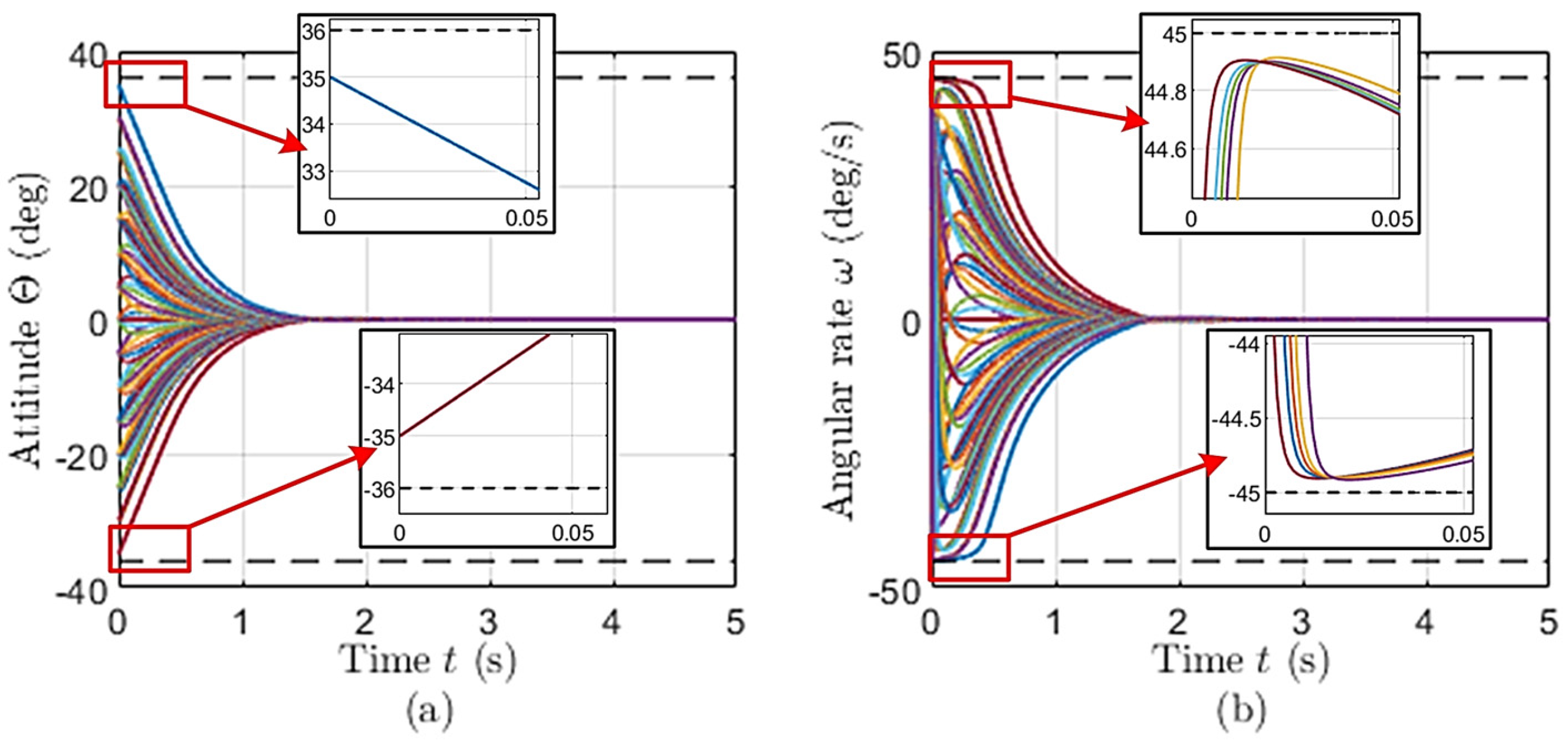
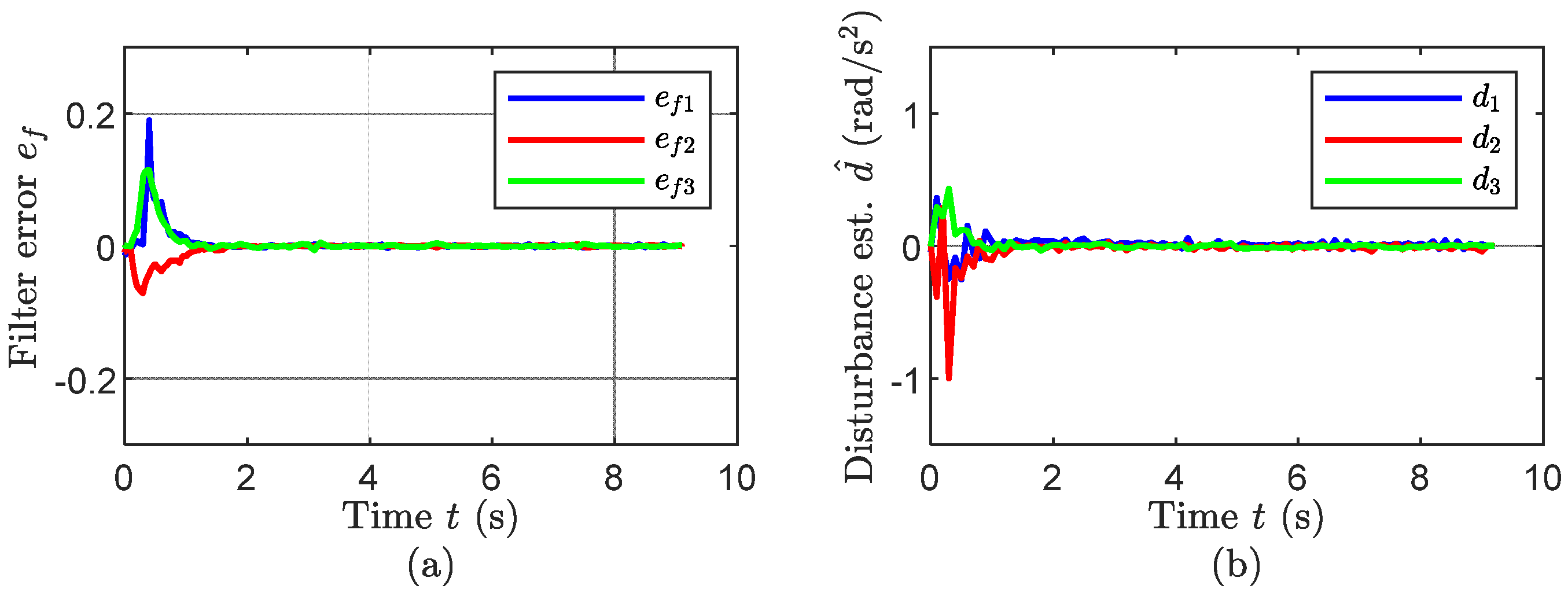
4.2. Finite-Time Convergence Validation

In this subsection, the finite-time convergence of the quadcopter’s attitude and angular rate will be examined and validated through conducting numerous simulations, making use of the dynamic model in (37), with different initial conditions. The initial values of the attitude range from −35 degrees to 35 degrees, while the initial angular rates range from −44 deg/s to 44 deg/s. It is worth noting that the boundaries of these ranges are intentionally set very close to the system constraints, i.e., $\pm 36$ degrees and $\pm 45$ deg/s for the attitudes and angular rates, respectively. Without the loss of generality, the desired attitudes and angular rates are set as zero. The simulation results will help to answer two questions, namely (i) whether the convergence time is bounded regardless of the initial conditions and (ii) whether the attitudes and angular rates strictly obey their given constraints.

The answer to the first question can be obtained easily from Figure 2. It is clear that, regardless of the initial values, the attitudes (Figure 2a) and angular rates (Figure 2b) converge rapidly to zero, and the convergence time is bounded by the value of 1.7 s, suggesting the efficacy of the proposed finite-time algorithm. However, this kind of performance is not something new as many other existing studies may also show similarity. Therefore, the answer to the second question will be crucial to emphasize the merits of this work. Looking at the inset in Figure 2a,b, it is seen that even though the initial values are set as $\pm 35$ degrees and $\pm 44$ deg/s, which are close to the given constraints, the attitudes and angular rate do not exceed such limits. This point is worth highlighting because many existing methods exhibit certain overshoots [32,33] that may result in breaking the constraints when the system’s states are near their limits.

4.3. Experimental Feasibility Validation

4.3.1. Experimental Setup

In order to validate the experimental feasibility and efficacy of the proposed algorithm, we conducted an experiment using an actual quadcopter platform (Figure 3). This platform is equipped with a propulsion system consisting of four pairs of 2312E-motors and a 9450-propeller [34]. The dynamic parameters of this platform are listed in

Table 1. Dynamic parameters of the experimental quadcopter UAV platform used in this work.

Parameter	Value	Unit
$J$	diag($[0.0119, 0.0131, 0.0232]$)	kg·m2
$l$	$0.225$	m
$c_t$	${10}^{-6}$	N·s2
$c_d$	$0.05$	-

. The flight control unit (FCU) utilizes the commercially available Pixhawk autopilot. This FCU consists of an onboard inertial navigation system (INS) that makes use of an IMU to provide measurements of the attitude and the angular rate. These measurements are used in the proposed algorithm. An RC receiver–transmitter pair is used for the initiation phase of each flight and for manual control as needed. Also, it has an onboard barometer and a LidarLite V3 laser scanner which provide altitude information to maintain the vehicle’s altitude in the air [2] (which is beyond the scope of this experiment and will not be described here). The proposed algorithm is implemented as an attitude controller into the FCU and is operated at a frequency of 400 Hz (Figure 4).

The experiment scenario is described as follows. The vehicle is initiated and armed on the ground. Then, it is taken off manually, by our pilot, to reach an altitude of 7 m, which is high enough to avoid the ground effect and low enough to avoid unexpectedly devastating crashes. While it is at the desired altitude and gets stabilized, the proposed algorithm is triggered. The quadcopter is commanded to autonomously reach the given attitude and angular rate references, i.e., $x_{d1}=(25, -25, 30)$ degrees and $x_{d2}=(0, 0, 0)$ deg/s (

Table 2. Parameters of the proposed disturbance observer, filter, and controller.

Parameter	Value
$c_1$	${[\pi /5, \pi /5, \pi /5]}^T$rad
$c_2$	${[\pi /4, \pi /4, \pi /4]}^T$rad/s
$x_{d1}$	${[5\pi /36, -5\pi /36, \pi /6]}^T$rad
$x_{d2}$	0 rad/s
$\alpha$	0.7
$[{\lambda }_i, {\lambda }_i^{\prime }, {\lambda }_i^{″}]$	$[5, 1, 2]$
$[{\gamma }_1, {\gamma }_2]$	$[0.1, 0.01]$
${\tau }_i$	$0.01$
$[{\chi }_{1i}, {\chi }_{2i}]$	$[0.7, 1.5]$
$[k_{11i}, k_{12i}, k_{21i}, k_{22i}]$	$[1, 2, 10, 30]$

). It is worth noting that while the quadcopter’s body is tilting, it is moving simultaneously. Therefore, after it completes the tracking, manual control will take over again to ensure that the vehicle will not hit the testing site’s barriers, noting that our testing site is not very large.

4.3.2. Experimental Results and Discussions

This subsection describes how the vehicle responds to the given commands and our discussions on such responses. As shown in Figure 5, after being triggered, the proposed algorithm actively steers the vehicle to get the references. It is seen that the quadcopter takes 1.2 s to reach all the attitude setpoints (Figure 5a). During the transient time and settling time, all attitude values remain within their given limits (the black dashed lines).

After approaching the references, the attitude tracking errors, representing the discrimination between the actual attitude and the given reference values, remain within the amplitude of 0.8 degree (Figure 5b). These minimal steady-state errors indicate an effective tracking performance. Moreover, the angular rates also quickly converge to zero and stay there with slight fluctuations (Figure 5c). Here, it is worth highlighting that, despite the fast convergence of attitude performance, the angular rates strictly follow the given constraints as they do not exceed their limits. Regarding the control inputs, it is seen in Figure 5d that the torques show a sharp transient effort to quickly drive the system to the references. After the transients, all the torques stabilize with small amplitudes.

Figure 6 depicts the performance of the proposed filter and disturbance observer. In Figure 6a, the filter errors exhibit small initial transients but quickly converge to zero within approximately 1.2 s, indicating accurate estimation and filter stability. Moreover, in Figure 6b, we can see the disturbance estimates also converge smoothly to steady ranges within a short time frame. This fast convergence suggests that the disturbance observer successfully compensates for unknown external factors, enhancing the robustness of the overall control system.

To demonstrate the effectiveness of the proposed method, a comparative analysis was conducted focusing on the convergence speed, overshoot, and steady-state error. The comparison considers two recently published studies [32,33] on the finite-time control of UAVs under full-state constraints. Since [32] reports only simulation results and [33] provides only experimental data, we compare our corresponding simulation and experimental results with those presented in each respective study. As shown in

Table 3. Comparison in terms of the convergence time, overshoot, and steady-state error of the attitude tracking control performance.

Criteria	Convergence Time [s]	Overshoot [deg]	Steady-State Error [deg]
[32] (simulation)	2.0	5.7	0
[33] (experiment)	3.5	2.9	1.2
Proposed (simulation)	1.7	0	0
Proposed (experiment)	1.2	0	0.8

, our proposed algorithm consistently achieves faster convergence, along with a significantly reduced overshoot and steady-state error, in both simulation and experimental settings compared to the referenced methods.

In summary, the proposed algorithm demonstrates accurate attitude tracking control performance with fast transient response and constraint satisfaction. While the attitude tracking errors rapidly decay and remain minimal, the angular rates guarantee the constraint obedience and show well-damped dynamics. This high performance can be achieved thanks to the combination of the proposed disturbance observer, filter, and backstepping controller. Overall, our method provides robust and stable attitude and angular rate tracking for the quadcopter.

5. Conclusions

To address the attitude tracking control problem for a second-order mechanical system subject to full-state constraints, this paper proposes an approach that integrates a finite-time, unknown-input, nonlinear disturbance observer with a backstepping control scheme augmented with a fast-converging finite-time filter. This design retains the advantages of the backstepping technique, such as a rapid response, straightforward design, and ease of implementation, while mitigating its inherent “explosion of complexity” issue. Furthermore, the finite-time, unknown-input, nonlinear disturbance observer enables effective compensation for external disturbances. Theoretical analyses were strictly conducted to assess the stability of the closed-loop system. To demonstrate the applicability of this method, it was applied to the attitude tracking control of a UAV. The experimental results confirm the feasibility and effectiveness of the proposed approach, demonstrating the accurate attitude tracking of the UAV in real flight conditions. Future work will involve the application of the proposed algorithm in different mechanical systems to examine its scalability.

References

1. Clark, R.N. Control System Dynamics; Cambridge University Press: Cambridge, UK, 1996. [Google Scholar]
2. Xuan-Mung, N.; Nguyen, N.P.; Pham, D.B.; Dao, N.-N.; Nguyen, H.T.; Ngoc, T.H.L.N.; Vu, M.T.; Hong, S.K. Novel gain-tuning for sliding mode control of second-order mechanical systems: Theory and experiments. Sci. Rep. 2023, 13, 10541. [Google Scholar] [CrossRef] [PubMed]
3. Khalil, H. Nonlinear Systems; Prentice Hall: Saddle River, NJ, USA, 2002. [Google Scholar]
4. Guo, K.; Zhang, H.; Wei, C. Novel sliding mode control of the manipulator based on a nonlinear disturbance observer. Sci. Rep. 2024, 14, 30656. [Google Scholar] [CrossRef] [PubMed]
5. Xuan-Mung, N.; Golestani, M. Energy-Efficient Disturbance Observer-Based Attitude Tracking Control With Fixed-Time Convergence for Spacecraft. IEEE Trans. Aerosp. Electron. Syst. 2023, 59, 3659–3668. [Google Scholar] [CrossRef]
6. Nguyen, N.; Park, D.; Ngoc, D.; Xuan-Mung, N.; Huynh, T.; Nguyen, T.; Hong, S. Quadrotor Formation Control via Terminal Sliding Mode Approach: Theory and Experiment Results. Drones 2022, 6, 172. [Google Scholar] [CrossRef]
7. Wang, D.; Pan, Q.; Shi, Y.; Hu, J.; Zhao, C. Efficient Nonlinear Model Predictive Control for Quadrotor Trajectory Tracking: Algorithms and Experiment. IEEE Trans. Cybern. 2021, 51, 5057–5068. [Google Scholar] [CrossRef]
8. Zheng, K.; Zhang, Q.; Hu, Y.; Wu, B. Design of fuzzy system-fuzzy neural network-backstepping control for complex robot system. Inf. Sci. 2021, 546, 1230–1255. [Google Scholar] [CrossRef]
9. Cordeiro, R.A.; Azinheira, J.R.; Moutinho, A. Robustness of Incremental Backstepping Flight Controllers: The Boeing 747 Case Study. IEEE Trans. Aerosp. Electron. Syst. 2021, 57, 3492–3505. [Google Scholar] [CrossRef]
10. Liu, Y.; Duan, C.; Liu, L.; Cao, L. Discrete-Time Incremental Backstepping Control with Extended Kalman Filter for UAVs. Electronics 2023, 12, 3079. [Google Scholar] [CrossRef]
11. Humaidi, A.; Hameed, M. Development of a New Adaptive Backstepping Control Design for a Non-Strict and Under-Actuated System Based on a PSO Tuner. Information 2019, 10, 38. [Google Scholar] [CrossRef]
12. Xuan-Mung, N.; Golestani, M. Smooth, singularity-free, finite-time tracking control for Euler–Lagrange systems. Mathematics 2022, 10, 3850. [Google Scholar] [CrossRef]
13. Xuan-Mung, N.; Hong, S.K. Robust Backstepping Trajectory Tracking Control of a Quadrotor with Input Saturation via Extended State Observer. Appl. Sci. 2019, 9, 5184. [Google Scholar] [CrossRef]
14. Zuo, Z.; Liu, C.; Han, Q.-L.; Song, J. Unmanned Aerial Vehicles: Control Methods and Future Challenges. IEEE/CAA J. Autom. Sin. 2022, 9, 601–614. [Google Scholar] [CrossRef]
15. Liu, Y.; Liu, X.; Jing, Y.; Chen, X.; Qiu, J. Direct Adaptive Preassigned Finite-Time Control With Time-Delay and Quantized Input Using Neural Network. IEEE Trans. Neural Netw. Learn. Syst. 2020, 31, 1222–1231. [Google Scholar] [CrossRef]
16. Guo, W.; Liu, D. Adaptive second-order backstepping control for a class of 2DoF underactuated systems with input saturation and uncertain disturbances. Sci. Rep. 2024, 14, 601–614. [Google Scholar] [CrossRef]
17. Liu, Y.; Li, H.; Lu, R.; Zuo, Z.; Li, X. An Overview of Finite/Fixed-Time Control and Its Application in Engineering Systems. IEEE/CAA J. Autom. Sin. 2022, 9, 2106–2120. [Google Scholar] [CrossRef]
18. Xuan-Mung, N.; Hong, S.K. Robust adaptive formation control of quadcopters based on a leader–follower approach. Int. J. Adv. Robot. Syst. 2019, 16, 1729881419862733. [Google Scholar] [CrossRef]
19. Nguyen, V.C.; Kim, S.H. A novel fixed-time prescribed performance sliding mode control for uncertain wheeled mobile robots. Sci. Rep. 2021, 11, 5340. [Google Scholar] [CrossRef]
20. Wang, C.; Li, S.; Ge, S.S. Finite-time sliding mode disturbance observer-based control for uncertain systems. Nonlinear Dyn. 2023, 111, 2191–2206. [Google Scholar]
21. Ho, C.M.; Tran, D.T.; Nguyen, C.H.; Ahn, K.K. Adaptive Neural Command Filtered Control for Pneumatic Active Suspension with Prescribed Performance and Input Saturation. IEEE Access 2021, 9, 56855–56868. [Google Scholar] [CrossRef]
22. Zhou, Y.; Lin, C.; Zhang, H. Finite-time adaptive fuzzy backstepping control with command filter and dynamic surface technique. ISA Trans. 2020, 99, 406–416. [Google Scholar]
23. Yu, J.; Shi, P.; Chen, X.; Cui, G. Finite-time command filtered adaptive control for uncertain nonlinear systems with actuator faults. IEEE Trans. Syst. Man Cybern. Syst. 2021, 51, 4098–4109. [Google Scholar]
24. Hajnorouzali, Y.; Malekzadeh, M.; Ataei, M. Finite-time disturbance observer based-control of flexible spacecraft. J. Vib. Control 2021, 29, 346–361. [Google Scholar] [CrossRef]
25. Chen, J.; Zhang, C.; Hu, J. Adaptive finite-time disturbance observer-based control for robotic systems with unknown dynamics. IEEE Trans. Control Syst. Technol. 2023, 31, 1581–1592. [Google Scholar]
26. Zhang, H.; Chen, X.; Xie, L. Finite-time adaptive tracking control of nonlinear systems with bounded disturbances and unmodeled dynamics. IEEE Trans. Ind. Electron. 2021, 68, 1418–1428. [Google Scholar]
27. Zuo, Z. Nonsingular fixed-time consensus tracking for second-order multi-agent networks. Automatica 2015, 54, 305–309. [Google Scholar] [CrossRef]
28. Hu, Q.; Jiang, B.; Zhang, Y. Observer-Based Output Feedback Attitude Stabilization for Spacecraft with Finite-Time Convergence. IEEE Trans. Cont. Syst. Tech. 2019, 27, 781–789. [Google Scholar] [CrossRef]
29. Polyakov, A. Nonlinear feedback design for fixed-time stabilization of linear control systems. IEEE Trans. Autom. Control 2012, 57, 2106–2110. [Google Scholar] [CrossRef]
30. Tian, B.; Zuo, Z.; Yan, X.; Wang, H. A fixed-time output feedback control scheme for double integrator systems. Automatica 2017, 80, 17–24. [Google Scholar] [CrossRef]
31. Xuan-Mung, N.; Hong, S. Quadcopter Precision Landing on Moving Targets via Disturbance Observer-Based Controller and Autonomous Landing Planner. IEEE Access 2022, 10, 83580–83590. [Google Scholar] [CrossRef]
32. Zhang, W.; Zhao, L. Command Filtered Backstepping Based Finite-Time Adaptive Fuzzy Event-Triggered Control for Unmanned Aerial Vehicle with Full-State Constraints. IEEE Trans. Veh. Technol. 2025, 1–13. [Google Scholar] [CrossRef]
33. Xiuyu, Z.; Li, H.; Zhu, G.; Zhang, Y.; Wang, C.; Wang, Y.; Su, C.-Y. Finite-Time Adaptive Quantized Control for Quadrotor Aerial Vehicle with Full States Constraints and Validation on QDrone Experimental Platform. Drones 2024, 8, 264. [Google Scholar] [CrossRef]
34. DJI. E305. Available online: http://www.dji.com/product/e305 (accessed on 30 April 2024).
Figure 1. The quadcopter’s angular rate, ω , is a measure in the body-fixed system ( O B x B y B z B ) , while the attitude, Θ , is in the earth-fixed ( O E x E y E z E ) coordinate system.
Mathematics 13 01810 g001
Figure 2. The attitude (a) and angular rate (b) convergences, corresponding to different initial conditions.
Mathematics 13 01810 g002
Figure 3. The experimental quadcopter UAV platform used for the illustrative case study in this paper.
Mathematics 13 01810 g003
Figure 4. The signal flow in the implementation of the proposed algorithm into the attitude control system of the quadcopter UAV.
Mathematics 13 01810 g004
Figure 5. Attitude tracking performance responding to step attitude references. (a) The attitude reaches its reference while remaining in the given constraints. (b) The attitude tracking errors converge to the origin without any overshoot. (c) The angular rate does not exceed the prescribed constraints. (d) The control inputs exhibit stable convergence.
Mathematics 13 01810 g005
Figure 6. The filter errors, after exhibiting overshoots for a short period of time, converge to zero and remain minimal (a). The disturbance estimation also shows the stable converging performance (b).
Mathematics 13 01810 g006