Mathematical Modeling and Analysis of Human-to-Human Transmitted Viral Encephalitis

Abstract

Encephalitis, a severe neurological condition caused by human-to-human (H2H) transmitted viruses, such as herpes simplex virus (HSV), requires a rigorous mathematical framework to understand its transmission dynamics. This study develops a nonlinear compartmental model, SEITR (Susceptible–Exposed–Infected–Treated–Recovered), to characterize the progression of viral encephalitis. The basic reproduction number (R₀) is derived using the next-generation matrix method, serving as a threshold parameter determining disease persistence. The local and global stability of the disease-free and endemic equilibria are established through a rigorous mathematical analysis. Additionally, a sensitivity analysis quantifies the impact of key parameters on R₀, offering more profound insights into their mathematical significance. Numerical simulations validate the theoretical results, demonstrating the system’s dynamical behavior under varying epidemiological conditions. This study provides a mathematically rigorous approach to modeling viral encephalitis transmission, filling a gap in the literature and offering a foundation for future research in infectious disease dynamics.

1. Introduction

Encephalitis is a severe neurological condition characterized by inflammation of the brain, primarily caused by viral infections. Various transmission routes contribute to its spread, including vector-borne, airborne, respiratory, sexual, and zoonotic pathways [1,2]. Among the causative agents, the herpes simplex virus (HSV), particularly HSV-1 and HSV-2, is a leading cause of viral encephalitis. HSV-1 is primarily transmitted through oral-to-oral contact, whereas HSV-2 spreads via sexual contact, leading to genital infections. Both types can result in encephalitis, a potentially life-threatening condition if left untreated [3,4].

Globally, HSV-1 affects approximately 3.8 billion people under the age of 50, while HSV-2 infects around 519.5 million individuals aged 15–49, making these viruses a significant public health concern [5]. Although the exact pathways by which these viruses reach the brain remain uncertain, transmission through the bloodstream or along nerve pathways has been hypothesized [6,7].

Past viral epidemics, including SARS, the Nipah virus, and COVID-19, have demonstrated the critical role of mathematical modeling in understanding disease dynamics and guiding public health strategies [8,9,10,11,12]. Models utilizing dynamical systems, stochastic processes, and network-based approaches have been instrumental in predicting outbreaks and optimizing control measures [13,14,15,16,17].

During the SARS outbreak, mathematical models informed epidemic control strategies [18,19,20], while for the Nipah virus, they played a crucial role in shaping containment policies in affected regions [21,22,23]. Advances in fractional-order models and optimal control approaches have further improved our understanding of viral kinetics and immune response [24,25,26,27].

For COVID-19, recent studies have provided deeper insights. Borah analyzed the simultaneous spread of multiple strains, while Dehingia developed a within-host delay differential model incorporating antiviral responses [28,29]. Nath et al. explored fractional-order dynamics in SARS-CoV-2 kinetics, offering new perspectives on viral persistence [30]. These advancements reinforce the importance of mathematical modeling in controlling infectious diseases.

Recent developments in mathematical modeling have integrated multiple transmission mechanisms and control measures. For instance, Zhang et al. explored delayed virus models with dual transmission pathways, while Tyagi et al. developed frameworks for managing the spread of infectious diseases [31,32]. Such models are essential for devising effective public health strategies, optimizing responses, and efficiently allocating healthcare resources during outbreaks [33,34,35].

Despite the substantial progress in the mathematical modeling of infectious diseases, there is a notable gap in the literature regarding the formulation of models for brain encephalitis, particularly focusing on human-to-human (H2H) transmission. Most existing models focus on vector-borne transmission dynamics, leaving H2H transmission largely unexplored. Given the complexity of viral encephalitis, which often involves varying incubation periods, asymptomatic carriers, and multiple transmission routes, there is a critical need for more comprehensive mathematical models that can integrate these variables and accurately simulate transmission dynamics [36,37,38,39,40].

In response to these gaps, this study aims to develop a comprehensive mathematical model to investigate the transmission dynamics of viral encephalitis, focusing specifically on the herpes simplex virus. The objectives of this study include the following:

❖

A model will be proposed that captures the nonlinear interaction between HSV and the development of brain encephalitis, considering various transmission factors.

❖

The primary reproduction number will be calculated using the next-generation matrix technique, and its impact on different compartments will be explored.

❖

The influence of model parameters on dependent variables will be assessed to identify key factors affecting disease dynamics and inform intervention strategies.

❖

The stability of the disease transmission process will be evaluated through the local and global stability of the disease-free equilibrium.

❖

The model will be visually represented using data-fitting techniques to depict disease dynamics under various scenarios.

❖

A comparative analysis of parameter values will be conducted to examine their effects on transmission dynamics and to guide effective public health interventions.

By addressing these gaps, this study aims to contribute to a more thorough understanding of the transmission dynamics of viral encephalitis, with a particular emphasis on human-to-human transmission, and to inform public health strategies and outbreak preparedness.

The document is structured as follows: Section 2 outlines the mathematical formulation of the proposed compartmental model. Section 3 presents a fundamental analysis of the model, employing the next-generation matrix technique and sensitivity analysis to determine the basic reproduction number. The stability of the model, both locally and globally, is explored in Section 4. Section 5 offers numerical simulations to support and validate the analytical results. Finally, Section 6 concludes with observations and insights derived from the study.

2. Mathematical Model

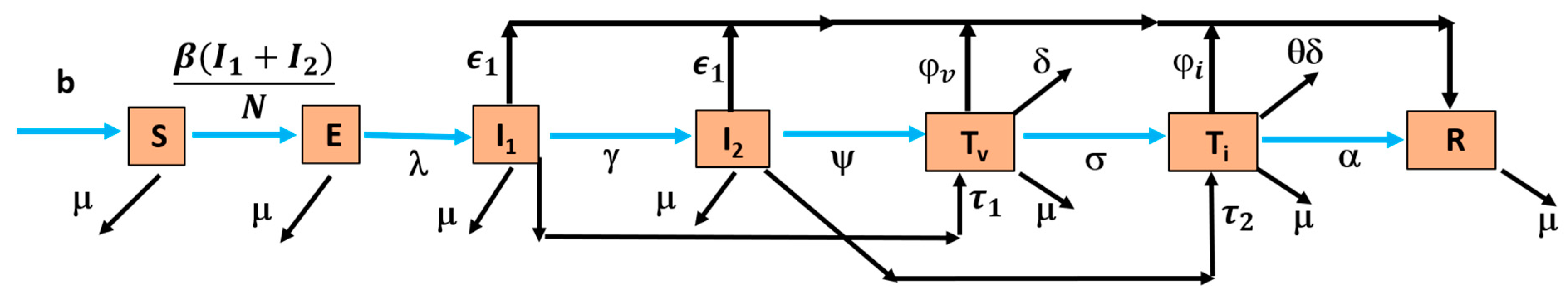
The nonlinear mathematical model investigates the effects of herpes simplex virus (HSV-1 and HSV-2) on brain encephalitis by categorizing the population, N(t), into seven mutually exclusive compartments to capture the progression and treatment dynamics of the disease. These compartments include susceptible individuals S(t), at risk of contracting the virus; exposed individuals E(t), infected but not yet infectious during the incubation period; asymptomatic individuals at an early stage I₁(t), who carry and transmit the virus without visible symptoms; symptomatic individuals at a later stage I₂(t), who develop clinical symptoms, like fever and seizures, and contribute significantly to transmission; individuals undergoing mechanical ventilation treatment T_v(t), requiring respiratory support due to severe complications; individuals undergoing ICU treatment T_i(t), receiving high-level care for life-threatening conditions; and recovered individuals R(t), who have resolved the infection and may develop immunity. This model effectively illustrates the disease’s progression, enabling targeted interventions and resource allocation for managing HSV-1 and HSV-2 encephalitis. The transmission diagram of the model is depicted in Figure 1. Consequently, the model captures the dynamic interactions among these compartments to understand the progression of the disease.

N(t) = S(t) + E(t) + I₁(t) +I₂(t) +T_v(t)+T_i(t) +R(t)

(1)

The set of deterministic equations governing the model is as follows. When individuals contract the infection through contact with infected individuals at a rate represented by b, it increases the population of susceptible individuals, S(t), by ${\displaystyle \frac{\beta \left({\mathrm{I}}_1+{\mathrm{I}}_2\right)}{\mathrm{N}}}$. Additionally, there is a contribution from natural death at a uniform rate ($\mu )$ consistent in all compartments. Thus, the equations capture the dynamics of the system accounting for both infection transmission and natural mortality:

$${\displaystyle \frac{\mathrm{d}\mathrm{S}}{\mathrm{d}\mathrm{t}}}=\mathrm{b}\mathrm{N}-{\displaystyle \frac{\beta \mathrm{S}({\mathrm{I}}_1+{\mathrm{I}}_2)}{\mathrm{N}}}-\mu \mathrm{S}$$

(2)

Afterward, exposed persons E(t) are produced by vulnerable individuals who contact infected individuals at a sure rate ${\displaystyle \frac{\beta \left({\mathrm{I}}_1+{\mathrm{I}}_2\right)}{\mathrm{N}}}$ and decreased at the rate $\lambda$, as well as by the natural death rate $\mu$, due to exposed persons who went on to become asymptomatic individuals I₁(t).

$${\displaystyle \frac{\mathrm{d}\mathrm{E}}{\mathrm{d}\mathrm{t}}}={\displaystyle \frac{\beta \mathrm{S}({\mathrm{I}}_1+{\mathrm{I}}_2)}{\mathrm{N}}}-\lambda \mathrm{E}-\mu \mathrm{E}$$

(3)

Individuals exposed at the early stage I₁(t) progressed to asymptomatic individuals at a rate of $\lambda$, while those who went to symptomatic individuals at the later stage I₂(t) at a rate of $\gamma$ reduced the asymptomatic individuals. This compartment was also reduced by the individuals who recovered spontaneously due to high antibody production at a rate of ${\epsilon }_1$, the rate of natural death at $\mu$, and the rate of asymptomatic individuals receiving antiviral therapy.

$${\displaystyle \frac{\mathrm{d}{\mathrm{I}}_1}{\mathrm{d}\mathrm{t}}}=\lambda \mathrm{E}-\gamma {\mathrm{I}}_1-{\epsilon }_1{\mathrm{I}}_1-\mu {\mathrm{I}}_1-{\tau }_1{\mathrm{I}}_1$$

(4)

The transition of asymptomatic individuals progressing to the symptomatic stage at a rate $\gamma$ and symptomatic individuals advancing to the treatment class, specifically under mechanical ventilation T_v(t), at a rate $\psi$ contributes to the population of individuals in the symptomatic stage at the later stage, denoted as I₂(t).

The asymptomatic individuals who progressed to symptomatic at a rate $\gamma$ and the symptomatic individuals who advanced to treatment class under mechanical ventilation T_v(t) at a rate$\psi$ use the symptomatic persons at the later stage I₂(t). This population was reduced by individuals who died naturally at the rate of $\mu$, recovered spontaneously due to potent antibodies at the rate of ${\epsilon }_1$, and received antiviral therapy for symptoms at the rate of ${\tau }_2$.

$${\displaystyle \frac{\mathrm{d}{\mathrm{I}}_2}{\mathrm{d}\mathrm{t}}}=\gamma {\mathrm{I}}_1-\psi {\mathrm{I}}_2-{\epsilon }_1{\mathrm{I}}_2-\mu {\mathrm{I}}_2-{\tau }_2{\mathrm{I}}_2$$

(5)

The treatment class with mechanical ventilation, represented by T_v(t), is influenced by symptomatic individuals advancing to the treatment class at a rate $\psi$ and the rate of antiviral therapy for asymptomatic individuals, denoted as I₁(t).

The class undergoing treatment with mechanical ventilation, denoted as T_v(t), results from the progression of symptomatic individuals to the treatment class at a rate $\psi$ and the administration of antiviral therapy to asymptomatic individuals, represented by I₁(t). This compartment is decreased by the patients who moved on to the treatment class under the intensive care unit T_i(t) at a rate of $\sigma$. It is also decreased by the patients who recovered due to ventilation at a rate of ${\phi }_{\mathrm{v}}$, by the natural death rate of $\mu$, and by the disease-induced death rate of $\delta$.

$${\displaystyle \frac{\mathrm{d}{\mathrm{T}}_{\mathrm{v}}}{\mathrm{d}\mathrm{t}}}=\psi {\mathrm{I}}_2+{\tau }_1{\mathrm{I}}_1-\sigma {\mathrm{T}}_{\mathrm{V}}-{\phi }_{\mathrm{v}}{\mathrm{T}}_{\mathrm{V}}-\mu {\mathrm{T}}_{\mathrm{V}}-\delta {\mathrm{T}}_{\mathrm{V}}$$

(6)

The ICU’s therapy class treatment individuals under ventilation T_i(t) who advanced to this treatment class at an $\sigma$ and antiviral treatment rate in symptomatic individuals I₂(t) create T_i(t). Those who went to the treatment class under recovery people R(t) at a rate of $\alpha$ likewise lessen this compartment, as do those who recovered from ICU therapy at a rate of ${\phi }_{\mathrm{i}}$, those who died naturally at a rate of $\mu$, and those who died from disease-induced death at a rate of θ$\delta$.

$${\displaystyle \frac{\mathrm{d}{\mathrm{T}}_{\mathrm{i}}}{\mathrm{d}\mathrm{t}}}=\sigma {\mathrm{T}}_{\mathrm{V}}+{\tau }_2{\mathrm{I}}_2-\alpha {\mathrm{T}}_{\mathrm{i}}-{\phi }_{\mathrm{i}}{\mathrm{T}}_{\mathrm{i}}-\mu {\mathrm{T}}_{\mathrm{i}}-\theta \delta {\mathrm{T}}_{\mathrm{i}}$$

(7)

The population in the recovered class, denoted as R(t), is influenced by individuals advancing to this state due to treatment. This advancement occurs at rates represented by ${\phi }_{\mathrm{v}}$ and ${\phi }_{\mathrm{i}}$ for individuals treated in T_v(t) and T_i(t), respectively. Moreover, individuals in the asymptomatic and symptomatic classes who naturally recover contribute to this class at a rate of ${\epsilon }_1$. This transition also reduces the rate of natural death (μ).

$${\displaystyle \frac{\mathrm{d}\mathrm{R}}{\mathrm{d}\mathrm{t}}}=\alpha {\mathrm{T}}_{\mathrm{i}}+{\phi }_{\mathrm{v}}{\mathrm{T}}_{\mathrm{v}}+{\phi }_{\mathrm{i}}{\mathrm{T}}_{\mathrm{i}}+{\epsilon }_1{\mathrm{I}}_1+{\epsilon }_1{\mathrm{I}}_2-\mu \mathrm{R}$$

(8)

The deterministic system of the nonlinear differential equation that follows is the model for the dynamics of viral encephalitis transmission based on the formulation and assumption given before [32]. The following lists the parameters and related state variables.

$$\left.\begin{array}{c}{\displaystyle \frac{\mathrm{d}\mathrm{S}}{\mathrm{d}\mathrm{t}}}=\mathrm{b}\mathrm{N}-{\displaystyle \frac{\beta \mathrm{S}({\mathrm{I}}_1+{\mathrm{I}}_2)}{\mathrm{N}}}-\mu \mathrm{S}\\ {\displaystyle \frac{\mathrm{d}\mathrm{E}}{\mathrm{d}\mathrm{t}}}={\displaystyle \frac{\beta \mathrm{S}({\mathrm{I}}_1+{\mathrm{I}}_2)}{\mathrm{N}}}-\lambda \mathrm{E}-\mu \mathrm{E}\\ {\displaystyle \frac{\mathrm{d}{\mathrm{I}}_1}{\mathrm{d}\mathrm{t}}}=\lambda \mathrm{E}-\lambda {\mathrm{I}}_1-{\epsilon }_1{\mathrm{I}}_1-\mu {\mathrm{I}}_1-{\tau }_1{\mathrm{I}}_1\\ {\displaystyle \frac{\mathrm{d}{\mathrm{I}}_2}{\mathrm{d}\mathrm{t}}}=\lambda {\mathrm{I}}_1-\psi {\mathrm{I}}_2-{\epsilon }_1{\mathrm{I}}_2-\mu {\mathrm{I}}_2-{\tau }_2{\mathrm{I}}_2\\ {\displaystyle \frac{\mathrm{d}{\mathrm{T}}_{\mathrm{v}}}{\mathrm{d}\mathrm{t}}}=\psi {\mathrm{I}}_2+{\tau }_1{\mathrm{I}}_1-\sigma {\mathrm{T}}_{\mathrm{V}}-{\phi }_{\mathrm{v}}{\mathrm{T}}_{\mathrm{V}}-\mu {\mathrm{T}}_{\mathrm{V}}-\delta {\mathrm{T}}_{\mathrm{V}}\\ {\displaystyle \frac{\mathrm{d}{\mathrm{T}}_{\mathrm{i}}}{\mathrm{d}\mathrm{t}}}=\sigma {\mathrm{T}}_{\mathrm{V}}+{\tau }_2{\mathrm{I}}_2-\alpha {\mathrm{T}}_{\mathrm{i}}-{\phi }_{\mathrm{i}}{\mathrm{T}}_{\mathrm{i}}-\mu {\mathrm{T}}_{\mathrm{i}}-\theta \delta {\mathrm{T}}_{\mathrm{i}}\\ {\displaystyle \frac{\mathrm{d}\mathrm{R}}{\mathrm{d}\mathrm{t}}}=\alpha {\mathrm{T}}_{\mathrm{i}}+{\phi }_{\mathrm{v}}{\mathrm{T}}_{\mathrm{v}}+{\phi }_{\mathrm{i}}{\mathrm{T}}_{\mathrm{i}}+{\epsilon }_1{\mathrm{I}}_1+{\epsilon }_1{\mathrm{I}}_2-\mu \mathrm{R}\end{array}\right\}$$

(9)

In the model, the compartments are defined as follows: S represents susceptible individuals, E denotes exposed individuals, and I refer to the infected class, which includes both I₁ (asymptomatic individuals at an early stage) and I₂ (symptomatic individuals at a later stage). The T class represents treated individuals, which is a combination of T_v (mechanically ventilated individuals) and T_i (ICU-treated individuals). R represents recovered individuals, and N is the total population.

Initial values:

$$\begin{gathered} S\left(0\right)=S_0>0;E\left(0\right)=E_0>0;I_1\left(0\right)=I_{1_0}\ge 0 \\ {I}_2\left(0\right)=I_{2_0}\ge 0;{ T}_v\left(0\right)=T_{v_0}>0; T_i\left(0\right)=T_{i_0}>0 \\ R\left(0\right)=R_0\ge 0 \end{gathered}$$

3. Fundamental Analysis of the Model

If all state variables of a model remain positive for every time instance (t), or if the model’s solution is positive for all t ≥ 0, it is deemed epidemiologically relevant.

Theorem 1 

(Positivity and feasible region). The region D = {(S, E, I₁, I₂, T_v, T_i, R) ∈ ${\mathbb{R}}_{+}^7$: N ≤ ${\displaystyle \frac{b}{\mu }}$} ensures positivity of the state variables and bounds all solutions of the system ${\mathbb{R}}_{+}^7$.

Proof. 

By summing all state variables, we obtain

N(t) = S(t) + E(t) + I₁(t) +I₂(t) +T_v(t)+T_i(t) +R(t)

Analyzing the total population dynamics shows that N(t) is bounded by ${\displaystyle \frac{\mathrm{b}}{\mu }}$, and as $\mathrm{when}t\to \infty ,\mathrm{t}\mathrm{h}\mathrm{e}\mathrm{n} 0\le N \le {\displaystyle \frac{\mathrm{b}}{\mu }}$

Thus, the region D contains all solutions and maintains positivity. □

See Appendix A for the detailed proof.

3.1. Positivity and Boundedness of the Solution

Based on the human population, the state variables and related parameters in the model are always non-negative, t. For the state variables, we are now computing non-negative results.

Theorem 2. 

Consider the initial data as follows: {(S(0), E(0), I₁(0), I₂(0), T_v(0), T_i(0), R(0)) ≥ 0} ∈ ${\mathbb{R}}_{+}^7$; then, the dynamical system (9)’s solution set will always be positive. For all times t > 0, the model equations {(S(0), E(0), I₁(0), I₂(0), T_v(0), T_i(0), R(0)} with positive initial data will continue to be positive.

Proof. 

Using the first equation of the system

$$\begin{gathered} {\displaystyle \frac{\mathrm{d}\mathrm{S}}{\mathrm{d}\mathrm{t}}}=-\beta \mathrm{S}({\mathrm{I}}_1+{\mathrm{I}}_2)-\mu \mathrm{S}+\mathrm{b} \\ \Rightarrow {\displaystyle \frac{\mathrm{d}\mathrm{S}}{\mathrm{d}\mathrm{t}}}=\mathrm{b}-\{\beta \left({\mathrm{I}}_1+{\mathrm{I}}_2\right)+\mu \}\mathrm{S} \ge -\{\beta \left({\mathrm{I}}_1+{\mathrm{I}}_2\right)+\mu \}\mathrm{S} \\ \Rightarrow {\displaystyle \frac{\mathrm{d}\mathrm{S}}{\mathrm{d}\mathrm{t}}}\ge -\{\beta \left({\mathrm{I}}_1+{\mathrm{I}}_2\right)+ \mu \}\mathrm{S} \\ {\displaystyle \frac{\mathrm{d}\mathrm{S}}{\mathrm{d}\mathrm{t}}}\ge -\{\beta \left({\mathrm{I}}_1+{\mathrm{I}}_2\right)+ \mu \}\mathrm{S} \end{gathered}$$

By integrating both sides

$$\Rightarrow \mathrm{S}\left(\mathrm{t}\right)\ge \mathrm{S}\left(0\right){\mathrm{e}}^{-(\beta \left({\mathrm{I}}_1+{\mathrm{I}}_2\right)+\mu )\mathrm{t}}\ge 0$$

Similarly, we may prove that, E(t) > 0, I₁(t) > 0, I₂(t) > 0, T_v(t) > 0, T_i(t) > 0, R(t) > 0

The positivity and boundedness of the model ensure that it is mathematically and epidemiologically well-posed. These properties allow for a meaningful dynamical analysis within the feasible region D. □

See Appendix B for the detailed proof.

3.2. Positivity Equilibria and Basic Reproduction Number (R₀)

The system model declares two equilibria: an endemic equilibrium point

${\mathrm{E}}^{\mathrm{*}}$ = (${\mathrm{S}}^{\mathrm{*}}$, ${\mathrm{E}}^{\mathrm{*}}$, ${\mathrm{I}}_1^{\mathrm{*}}$, ${\mathrm{I}}_2^{\mathrm{*}}$, ${\mathrm{T}}_{\mathrm{v}}^{\mathrm{*}}$, ${\mathrm{T}}_{\mathrm{i}}^{\mathrm{*}}$, ${\mathrm{R}}^{\mathrm{*}}$) and a disease-free equilibria (DFE) point

E₀ = (S⁰, 0, 0, 0, 0, 0, 0) = (${\displaystyle \frac{\mathrm{b}}{\mu }}$, 0, 0, 0, 0, 0, 0).

The basic reproduction number, R₀, represents the average number of secondary infections generated by a single infected individual in a fully susceptible population. This metric is crucial for understanding the transmission dynamics of infectious diseases. To evaluate these dynamics, we employ the next-generation matrix method, where R₀ is determined as the next-generation matrix’s spectral radius (i.e., the largest eigenvalue). This approach provides a systematic framework for assessing disease spread and control measures (Shuai and Van Den Driessche [9]).

R₀ is the dominant eigenvalue of the matrix G = FV⁻¹

Ƒ = New infections and

ν = transfers of infections from one compartment to other

$$\mathbf{Ƒ}=\left(\begin{array}{c}\beta \mathrm{S}{\mathrm{I}}_1+{\beta \mathrm{S}\mathrm{I}}_2\\ 0\\ 0\end{array}\right)\hspace{1em}\hspace{1em}\hspace{1em}\hspace{1em} \nu =\left(\begin{array}{c}-\lambda \mathrm{E}-\mu \mathrm{E}\\ \begin{array}{c}\lambda E-\gamma {\mathrm{I}}_1-{\epsilon }_1{\mathrm{I}}_1-\mu {\mathrm{I}}_1-{\tau }_1{\mathrm{I}}_1\\ {\gamma \mathrm{I}}_1-{\psi {\mathrm{I}}_2-\epsilon }_1{\mathrm{I}}_2-\mu {\mathrm{I}}_2-{\tau }_2{\mathrm{I}}_2\end{array}\end{array}\right)$$

Constructing the F and V matrix,

$$\mathrm{F}=\mathrm{J}\mathrm{a}\mathrm{c}\mathrm{o}\mathrm{b}\mathrm{i}\mathrm{a}\mathrm{n} \mathrm{o}\mathrm{f} \mathbf{Ƒ}=\left(\begin{array}{ccc}{\displaystyle \frac{𝜕\mathrm{f}}{𝜕\mathrm{E}}}& {\displaystyle \frac{𝜕\mathrm{f}}{𝜕{\mathrm{I}}_1}}& {\displaystyle \frac{𝜕\mathrm{f}}{𝜕{\mathrm{I}}_2}}\\ {\displaystyle \frac{𝜕\mathrm{g}}{𝜕\mathrm{E}}}& {\displaystyle \frac{𝜕\mathrm{g}}{𝜕{\mathrm{I}}_1}}& {\displaystyle \frac{𝜕\mathrm{g}}{𝜕{\mathrm{I}}_2}}\\ {\displaystyle \frac{𝜕\mathrm{h}}{𝜕\mathrm{E}}}& {\displaystyle \frac{𝜕\mathrm{h}}{𝜕{\mathrm{I}}_1}}& {\displaystyle \frac{𝜕\mathrm{h}}{𝜕{\mathrm{I}}_2}}\end{array}\right)=\left(\begin{array}{ccc}0& \beta \mathrm{S}& \beta \mathrm{S}\\ 0& 0& 0\\ 0& 0& 0\end{array}\right)$$

where βS denotes the infection rate due to susceptible individuals interacting with the infected classes I₁ and I₂.

Let for V

$$\mathrm{V}=\mathrm{J}\mathrm{a}\mathrm{c}\mathrm{o}\mathrm{b}\mathrm{i}\mathrm{a}\mathrm{n} \mathrm{o}\mathrm{f} \nu =\left(\begin{array}{ccc}{\displaystyle \frac{𝜕\mathrm{f}}{𝜕\mathrm{E}}}& {\displaystyle \frac{𝜕\mathrm{f}}{𝜕{\mathrm{I}}_1}}& {\displaystyle \frac{𝜕\mathrm{f}}{𝜕{\mathrm{I}}_2}}\\ {\displaystyle \frac{𝜕\mathrm{g}}{𝜕\mathrm{E}}}& {\displaystyle \frac{𝜕\mathrm{g}}{𝜕{\mathrm{I}}_1}}& {\displaystyle \frac{𝜕\mathrm{g}}{𝜕{\mathrm{I}}_2}}\\ {\displaystyle \frac{𝜕\mathrm{h}}{𝜕\mathrm{E}}}& {\displaystyle \frac{𝜕\mathrm{h}}{𝜕{\mathrm{I}}_1}}& {\displaystyle \frac{𝜕\mathrm{h}}{𝜕{\mathrm{I}}_2}}\end{array}\right)=\left(\begin{array}{ccc}-\lambda -\mu & 0& 0\\ \lambda & -\gamma -{\epsilon }_1-\mu -{\tau }_1& 0\\ 0& \gamma & -\psi {-\epsilon }_1-\mu -{\tau }_2\end{array}\right)$$

$${\mathrm{V}}^{-1}=\left(\begin{array}{ccc}{\displaystyle \frac{1}{(\lambda +\mu )}}& 0& 0\\ {\displaystyle \frac{\lambda }{(\lambda +\mu )(\gamma +{\epsilon }_1+\mu +{\tau }_1)}}& {\displaystyle \frac{1}{(\gamma +{\epsilon }_1+\mu +{\tau }_1)}}& 0\\ {\displaystyle \frac{\lambda \gamma }{(\lambda +\mu )(\gamma +{\epsilon }_1+\mu +{\tau }_1)(\psi +{\epsilon }_1+\mu +{\tau }_2)}}& {\displaystyle \frac{\gamma }{(\gamma +{\epsilon }_1+\mu +{\tau }_1)(\psi +{\epsilon }_1+\mu +{\tau }_2)}}& {\displaystyle \frac{1}{(\psi +{\epsilon }_1+\mu +{\tau }_2)}}\end{array}\right)$$

$$\mathrm{F}{\mathrm{V}}^{-1}=\left(\begin{array}{ccc}{\displaystyle \frac{\beta \mathrm{s}\lambda }{(\lambda +\mu )(\gamma +{\epsilon }_1+\mu +{\tau }_1)}}+{\displaystyle \frac{\beta \mathrm{s}\lambda \gamma }{(\lambda +\mu )(\gamma +{\epsilon }_1+\mu +{\tau }_1)(\psi +{\epsilon }_1+\mu +{\tau }_2)}}& {\displaystyle \frac{\beta \mathrm{s}}{(\gamma +{\epsilon }_1+\mu +{\tau }_1)}}+{\displaystyle \frac{\beta \mathrm{s}\gamma }{(\gamma +{\epsilon }_1+\mu +{\tau }_1)(\psi +{\epsilon }_1+\mu +{\tau }_2)}}& {\displaystyle \frac{\beta \mathrm{s}}{(\psi +{\epsilon }_1+\mu +{\tau }_2)}}\\ 0& 0& 0\\ 0& 0& 0\end{array}\right)$$

Then, the basic reproduction number, R₀, which is the most immense eigenvalue of FV⁻¹ is

$${\mathrm{R}}_0={\displaystyle \frac{\beta \mathrm{s}\lambda }{(\lambda +\mu )(\gamma +{\epsilon }_1+\mu +{\tau }_1)}}\left(1+{\displaystyle \frac{\gamma }{\psi +{\epsilon }_1+\mu +{\tau }_2}}\right)={\displaystyle \frac{\beta \mathrm{s}\lambda (\psi +{\epsilon }_1+\mu +{\tau }_2+\gamma )}{(\lambda +\mu )(\gamma +{\epsilon }_1+\mu +{\tau }_1)(\psi +{\epsilon }_1+\mu +{\tau }_2)}}$$

This expression represents the threshold for disease transmission. If R₀ > 1, the disease can spread within the population; if R₀ < 1, the disease will eventually die out.

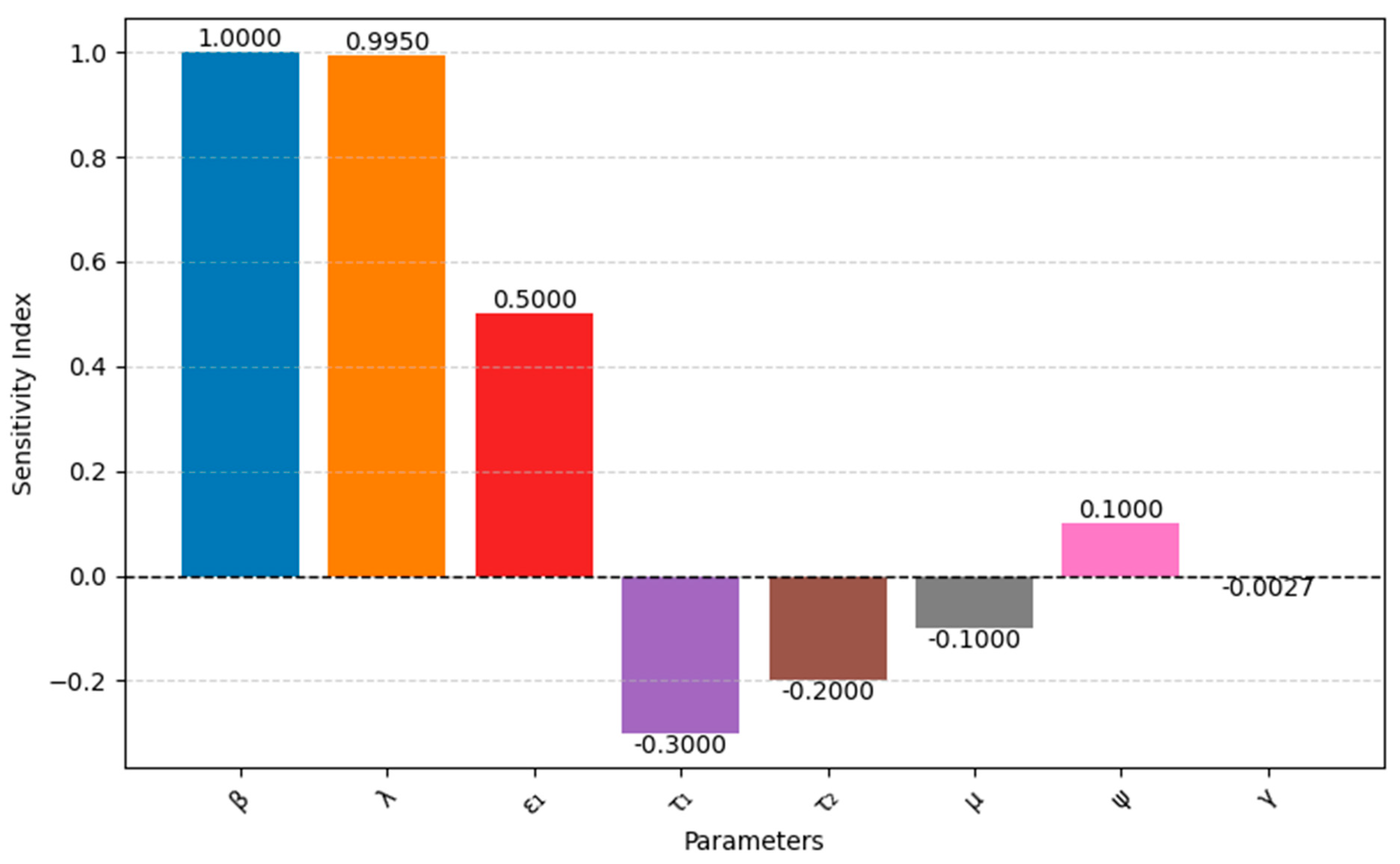
3.3. Sensitivity Analysis of R₀

We utilized a normalized sensitivity analysis to evaluate the influence of key parameters on the basic reproduction number (R₀). This approach involves calculating the sensitivity index, defined as ${\mathrm{Y}}_{\mathrm{P}}^{{\mathrm{R}}_0}={\displaystyle \frac{\mathrm{P}}{{\mathrm{R}}_0}}{\displaystyle \frac{𝜕{\mathrm{R}}_0}{𝜕\mathrm{P}}}$. A sensitivity analysis was performed to examine the effect of model parameters on the dependent variables in the model. This helps researchers understand how changes in a parameter contribute to increases or decreases in the state variables. The sensitivity index for R₀ is given by ${\mathrm{Y}}_{\mathrm{P}}^{{\mathrm{R}}_0}={\displaystyle \frac{\mathrm{P}}{{\mathrm{R}}_0}}{\displaystyle \frac{𝜕{\mathrm{R}}_0}{𝜕\mathrm{P}}}$.

The sensitivity index based on R₀ is given by

$${\mathrm{Y}}_{\mathrm{P}}^{{\mathrm{R}}_0}={\displaystyle \frac{\mathrm{P}}{{\mathrm{R}}_0}}{\displaystyle \frac{𝜕{\mathrm{R}}_0}{𝜕\mathrm{P}}}$$

where R₀ = Basic reproduction number

P = Parameter of interest

As we obtain in the compartmental model $R$₀$={\displaystyle \frac{\beta s\lambda (\psi +{\epsilon }_1+\mu +{\tau }_2+\gamma )}{(\lambda +\mu )(\gamma +{\epsilon }_1+\mu +{\tau }_1)(\psi +{\epsilon }_1+\mu +{\tau }_2)}}$

So, here, we compute the sensitivity index numerator index ${\displaystyle \frac{\beta s\lambda (\psi +{\epsilon }_1+\mu +{\tau }_2+\gamma )}{(\lambda +\mu )(\gamma +{\epsilon }_1+\mu +{\tau }_1)(\psi +{\epsilon }_1+\mu +{\tau }_2)}}$ of $\beta$ based on R₀

$$\begin{array}{c}\mathrm{a}\mathrm{v}\mathrm{a}\mathrm{i}\mathrm{l}\mathrm{a}\mathrm{b}\mathrm{l}\mathrm{e} {\mathrm{Y}}_{\beta }^{{\mathrm{R}}_0}={\displaystyle \frac{\beta }{{\mathrm{R}}_0}}{\displaystyle \frac{𝜕{\mathrm{R}}_0}{𝜕\beta }}\hfill \\ {\displaystyle \frac{𝜕{\mathrm{R}}_0}{𝜕\beta }}={\displaystyle \frac{\mathrm{s}\lambda }{(\lambda +\mu )(\gamma +{\epsilon }_1+\mu +{\tau }_1)}}\left(1+{\displaystyle \frac{\gamma }{\psi +{\epsilon }_1+\mu +{\tau }_2}}\right)\hfill \end{array}$$

$$\begin{array}{cc}\hfill \mathrm{available}& {\mathrm{Y}}_{\beta }^{{\mathrm{R}}_0}={\displaystyle \frac{\beta }{{\mathrm{R}}_0}}{\displaystyle \frac{\mathrm{s}\lambda }{(\lambda +\mu )(\gamma +{\epsilon }_1+\mu +{\tau }_1)}}\left(1+{\displaystyle \frac{\gamma }{\psi +{\epsilon }_1+\mu +{\tau }_2}}\right)\hfill \\ & \hspace{1em}={\displaystyle \frac{\beta (\lambda +\mu )(\gamma +{\epsilon }_1+\mu +{\tau }_1)(\psi +{\epsilon }_1+\mu +{\tau }_2)}{\beta \mathrm{s}\lambda (\psi +{\epsilon }_1+\mu +{\tau }_2+\gamma )}}{\displaystyle \frac{\mathrm{s}\lambda (\psi +{\epsilon }_1+\mu +{\tau }_2+\gamma )}{(\lambda +\mu )(\gamma +{\epsilon }_1+\mu +{\tau }_1)(\psi +{\epsilon }_1+\mu +{\tau }_2)}}\\ & \hspace{1em}=1\hfill \end{array}$$

Interpretation: The plus sign indicates a direct relationship between $\beta$ on R₀. The 1 means that a unit increase in $\beta$ will result in a unit increase in R₀.

Similarly, we calculate the parameters “$\lambda$ ”, “$\gamma$ ”, “${\epsilon }_1$”, “${\tau }_1$”, “${\tau }_2$”, “$\psi$ ”, and “$\mu$ ”. Figure 2 illustrates the sensitivity analysis of these parameters with respect to R₀.

3.4. Equilibrium Stability and Existence

An epidemiological model is called locally stable if the neighborhood point can quickly move to it within some time, and the model will be globally stable when it moves to the equilibrium point from any point of the model.

An epidemiological model must be stable (local or global stability). Here, we analyze the model for the stability property.

4. Disease-Free Model

Now, we study the model without treatment, which we obtain by considering.

$${\mathrm{T}}_{\mathrm{v}}={\mathrm{T}}_{\mathrm{i}}={\tau }_1={\tau }_2=\sigma =\psi ={\phi }_{\mathrm{v}}={\phi }_{\mathrm{i}}=0$$

$$\left.\begin{array}{c}{\displaystyle \frac{\mathrm{d}\mathrm{S}}{\mathrm{d}\mathrm{t}}}=\mathrm{b}-\beta \mathrm{S}\left({\mathrm{I}}_1+{\mathrm{I}}_2\right)-\mu \mathrm{S}\\ {\displaystyle \frac{\mathrm{d}\mathrm{E}}{\mathrm{d}\mathrm{t}}}=\beta \mathrm{S}\left({\mathrm{I}}_1+{\mathrm{I}}_2\right)-\lambda \mathrm{E}-\mu \mathrm{E}\\ {\displaystyle \frac{\mathrm{d}{\mathrm{I}}_1}{\mathrm{d}\mathrm{t}}}=\lambda \mathrm{E}-\gamma {\mathrm{I}}_1-{\epsilon }_1{\mathrm{I}}_1-\mu {\mathrm{I}}_1\\ {\displaystyle \frac{\mathrm{d}{\mathrm{I}}_2}{\mathrm{d}\mathrm{t}}}={\gamma \mathrm{I}}_1-{\epsilon }_1{\mathrm{I}}_2-\mu {\mathrm{I}}_2\\ {\displaystyle \frac{\mathrm{d}\mathrm{R}}{\mathrm{d}\mathrm{t}}}={\epsilon }_1{\mathrm{I}}_1+{\epsilon }_1{\mathrm{I}}_2-\mu \mathrm{R}\end{array}\right\}$$

(10)

The treatment-free model is positively invariant and attractive in region D₁ = {(S, E, I₁, I₂, R) ∈ ${\mathbb{R}}_{+}^5$: S + E + I₁ + I₂ + R $\le {\displaystyle \frac{\mathrm{b}}{\mu }}$}. Thus, considering t, the model’s dynamics is sufficient.

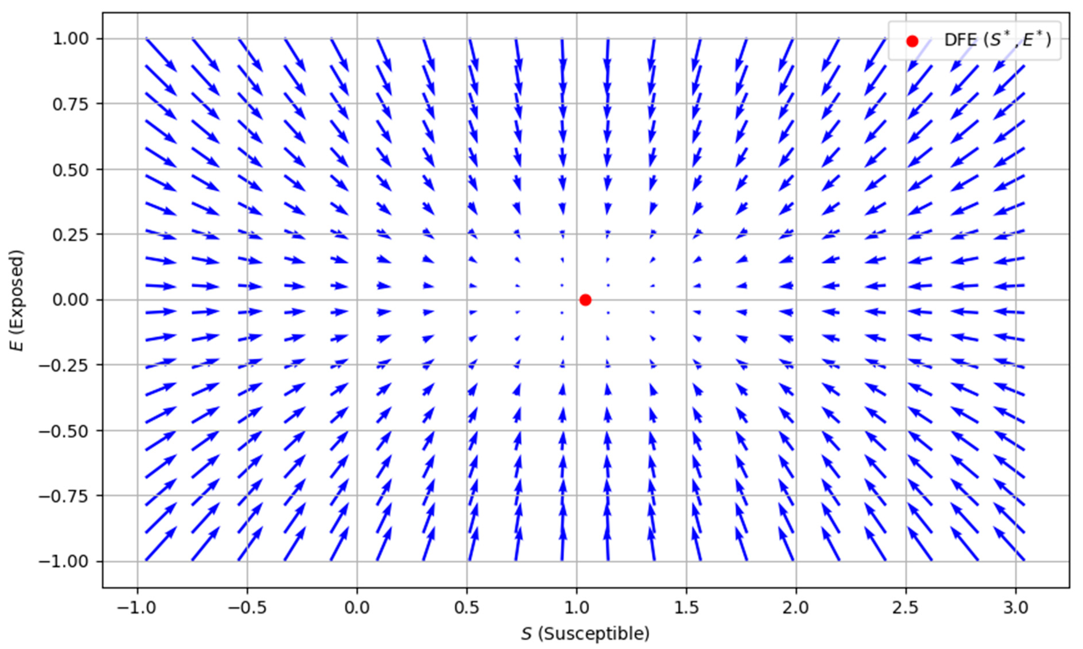
4.1. Existence of Disease-Free Equilibrium (DFE)

In a state of equilibrium where ${\mathrm{S}}^{\mathrm{*}}={\mathrm{E}}^{\mathrm{*}}={\mathrm{I}}_1^{\mathrm{*}}={\mathrm{I}}_2^{\mathrm{*}}={\mathrm{T}}_{\mathrm{v}}^{\mathrm{*}}={\mathrm{T}}_{\mathrm{i}}^{\mathrm{*}}={\mathrm{R}}^{\mathrm{*}}=0$, the absence of disease is established; a specific point is referred to as the disease-free equilibrium, which is

$${\epsilon }_0=({\mathrm{S}}^{\mathrm{*}}, {\mathrm{E}}^{\mathrm{*}}, {\mathrm{I}}_1^{\mathrm{*}}, {\mathrm{I}}_2^{\mathrm{*}}, {\mathrm{T}}_{\mathrm{v}}^{\mathrm{*}}, {\mathrm{T}}_{\mathrm{i}}^{\mathrm{*}}, {\mathrm{R}}^{\mathrm{*}})=({\displaystyle \frac{\mathrm{b}}{\mu }},0,0,0,0,0,0)$$

Figure 3 shows how the system behaves near the DFE. The DFE is stable, meaning that the disease is likely to die out if no infected individuals are introduced, and the population will return to a state where no one is exposed or infected. The vectors guide the system to this disease-free state, generally pointing toward equilibrium.

4.2. Local Stability of DFE

To analyze the system, we focus on the functional matrix representation. The matrices F and V are constructed by calculating the partial derivatives of the system’s rate functions with respect to the variables E, I₁, and I₂ capturing the dynamics of how each compartment influences the others.

$$Ƒ=\left(\begin{array}{c}\beta S{I}_1+{\beta SI}_2\\ 0\\ 0\end{array}\right)\hspace{1em}\hspace{1em}\hspace{1em}\hspace{1em} \nu = \left(\begin{array}{c}-\lambda E-\mu E\\ \begin{array}{c}\lambda E-\gamma I_1-{\epsilon }_1{I}_1-\mu I_1\\ {\gamma I}_1-{\epsilon }_1{I}_2-\mu I_2\end{array}\end{array}\right)$$

Constructing F and V matrix

Let for F f(E, I₁, I₂) = $\beta SI$; g(E, I₁, I₂) = 0; h(E, I₁, I₂) = 0

$$\mathrm{F}= \left(\begin{array}{ccc}{\displaystyle \frac{𝜕\mathrm{f}}{𝜕\mathrm{E}}}& {\displaystyle \frac{𝜕\mathrm{f}}{𝜕{\mathrm{E}}_1}}& {\displaystyle \frac{𝜕\mathrm{f}}{𝜕{\mathrm{E}}_2}}\\ {\displaystyle \frac{𝜕\mathrm{g}}{𝜕\mathrm{E}}}& {\displaystyle \frac{𝜕\mathrm{g}}{𝜕{\mathrm{I}}_1}}& {\displaystyle \frac{𝜕\mathrm{g}}{𝜕{\mathrm{I}}_2}}\\ {\displaystyle \frac{𝜕\mathrm{h}}{𝜕\mathrm{E}}}& {\displaystyle \frac{𝜕\mathrm{h}}{𝜕{\mathrm{I}}_1}}& {\displaystyle \frac{𝜕\mathrm{h}}{𝜕{\mathrm{I}}_2}}\end{array}\right) = \left(\begin{array}{ccc}0& \beta \mathrm{S}& \beta \mathrm{S}\\ 0& 0& 0\\ 0& 0& 0\end{array}\right)$$

$$\mathrm{V}= \left(\begin{array}{ccc}{\displaystyle \frac{𝜕\mathrm{f}}{𝜕\mathrm{e}}}& {\displaystyle \frac{𝜕\mathrm{f}}{𝜕{\mathrm{i}}_1}}& {\displaystyle \frac{𝜕\mathrm{f}}{𝜕{\mathrm{i}}_2}}\\ {\displaystyle \frac{𝜕\mathrm{g}}{𝜕\mathrm{e}}}& {\displaystyle \frac{𝜕\mathrm{g}}{𝜕{\mathrm{i}}_1}}& {\displaystyle \frac{𝜕\mathrm{g}}{𝜕{\mathrm{i}}_2}}\\ {\displaystyle \frac{𝜕\mathrm{h}}{𝜕\mathrm{e}}}& {\displaystyle \frac{𝜕\mathrm{h}}{𝜕{\mathrm{i}}_1}}& {\displaystyle \frac{𝜕\mathrm{h}}{𝜕{\mathrm{i}}_2}}\end{array}\right) = \left(\begin{array}{ccc}-\lambda -\mu & 0& 0\\ \lambda & -\gamma -{\epsilon }_1-\mu & 0\\ 0& \gamma & -{\epsilon }_1-\mu \end{array}\right)$$

$${\mathrm{V}}^{-1}=\left(\begin{array}{ccc}{\displaystyle \frac{1}{(\lambda +\mu )}}& 0& 0\\ {\displaystyle \frac{\lambda }{(\lambda +\mu )(\gamma +{\epsilon }_1+\mu )}}& {\displaystyle \frac{1}{(\gamma +{\epsilon }_1+\mu )}}& 0\\ {\displaystyle \frac{\lambda \gamma }{(\lambda +\mu )(\gamma +{\epsilon }_1+\mu )({\epsilon }_1+\mu )}}& {\displaystyle \frac{\gamma }{(\gamma +{\epsilon }_1+\mu )({\epsilon }_1+\mu )}}& {\displaystyle \frac{1}{({\epsilon }_1+\mu )}}\end{array}\right)$$

$$\mathrm{F}{\mathrm{V}}^{-1}= \left(\begin{array}{ccc}{\displaystyle \frac{\beta \mathrm{S}\lambda }{(\lambda +\mu )(\gamma +{\epsilon }_1+\mu )}}+{\displaystyle \frac{\beta \mathrm{S}\lambda \gamma }{(\lambda +\mu )(\gamma +{\epsilon }_1+\mu )({\epsilon }_1+\mu )}}& {\displaystyle \frac{\beta \mathrm{S}}{(\gamma +{\epsilon }_1+\mu )}}+{\displaystyle \frac{\beta \mathrm{S}}{(\gamma +{\epsilon }_1+\mu )({\epsilon }_1+\mu )}}& {\displaystyle \frac{\beta \mathrm{S}}{({\epsilon }_1+\mu )}}\\ 0& 0& 0\\ 0& 0& 0\end{array}\right)$$

So, $\mathrm{R}$₀$={\displaystyle \frac{\beta \mathrm{b}\lambda }{\mathrm{N}\mu (\lambda +\mu )({\epsilon }_1+\mu )}}$ =${\displaystyle \frac{\beta \mathrm{b}}{\mathrm{N}\mu }}{\displaystyle \frac{\lambda }{(\lambda +\mu )}}{\displaystyle \frac{1}{({\epsilon }_1+\mu )}}$.

In this case, the average duration of an infectious person is ${\displaystyle \frac{1}{({\epsilon }_1+\mu )}}$, the transmission probability is ${\displaystyle \frac{\beta \mathrm{b}}{\mathrm{N}\mu }}$ and the probability that a person has contracted an infectious disease is ${\displaystyle \frac{\lambda }{(\lambda +\mu )}}$.

Theorem 3. 

The H2H-transmitted viral encephalitis model is unstable if R₀ > 1 and locally asymptotically stable at disease-free equilibrium when R₀ < 1.

According to this biological theorem, H2H-transmitted brain encephalitis can be eliminated from society if the reproduction number is smaller than unity.

It is essential to demonstrate the global asymptotic stability of the DFE within the invariance region D₁. This proof is accomplished through the following methods.

4.3. Global Stability of DFE

Theorem 4. 

The DFE model is globally asymptotically stable if R₀ ≤ 1 and unstable if R₀ ≥ 1

Proof. 

Consider the following Lyapunov function, where we examine its properties and implications in the context of the system under consideration:

F = aE² + bI₁² + cI₂² where a, b, c > 0

After Lyapunov derivatives

$$\dot{\mathrm{F}}=2\mathrm{a}\mathrm{E}\dot{\mathrm{E}}+2\mathrm{b}{\mathrm{I}}_1\dot{{\mathrm{I}}_1}+\mathrm{c}{\mathrm{I}}_2\dot{{\mathrm{I}}_2}$$

A slight deviation from the reproduction number would

$${\mathrm{P}}_1=(\lambda +\mu ); {\mathrm{P}}_2=(\gamma +{\epsilon }_1+\mu ); {\mathrm{P}}_3=({\epsilon }_1+\mu )$$

Let here a = λP₃; b = P₁P₃; c = P₁.

$$\begin{gathered} \dot{\mathrm{F}}=2\mathrm{aE} \{\beta \mathrm{S}\left({\mathrm{I}}_1+{\mathrm{I}}_2\right)-{\mathrm{P}}_1\mathrm{E}\}+2\mathrm{b}{\mathrm{I}}_1(\lambda \mathrm{E}-{\mathrm{P}}_2{\mathrm{I}}_1)+2\mathrm{c}{\mathrm{I}}_2({\gamma \mathrm{I}}_1-{\mathrm{P}}_3{\mathrm{I}}_2) \\ \Rightarrow \dot{\mathrm{F}}=2\mathrm{a}\beta \mathrm{S}{\mathrm{I}}_1+{2\mathrm{a}\beta \mathrm{S}\mathrm{I}}_2-2\mathrm{a}{\mathrm{P}}_1{\mathrm{E}}^2+2\mathrm{b}{\mathrm{I}}_1\lambda \mathrm{E}-2\mathrm{b}{\mathrm{P}}_2{{\mathrm{I}}_1}^2+2\mathrm{c}{\gamma \mathrm{I}}_1{\mathrm{I}}_2-2\mathrm{c}{\mathrm{P}}_3{{\mathrm{I}}_2}^2 \\ \Rightarrow \dot{\mathrm{F}}=2\lambda \beta {\mathrm{P}}_3\mathrm{S}{\mathrm{I}}_1+{2\lambda {\mathrm{P}}_3\beta \mathrm{S}\mathrm{I}}_2-2\lambda {\mathrm{P}}_1{\mathrm{P}}_3{\mathrm{E}}^2+{2\lambda \mathrm{P}}_1{\mathrm{P}}_3{\mathrm{I}}_1\mathrm{E}-{2\mathrm{P}}_1{\mathrm{P}}_2{\mathrm{P}}_3{{\mathrm{I}}_1}^2+{2\mathrm{P}}_1{\gamma \mathrm{I}}_1{\mathrm{I}}_2-{2\mathrm{P}}_1{\mathrm{P}}_3{{\mathrm{I}}_2}^2 \end{gathered}$$

Using the definition of the basic reproduction number R₀, which is related to the model parameters. By factoring and simplifying

$$\dot{\mathrm{F}}={\mathrm{P}}_1{\mathrm{P}}_2{\mathrm{P}}_3({\mathrm{R}}_0-1){{\mathrm{I}}_1}^2+{\mathrm{P}}_1{\mathrm{P}}_2{\mathrm{P}}_3({\mathrm{R}}_0-1){{\mathrm{I}}_2}^2$$

If R₀ ≤ 1 then $\dot{\mathrm{F}}$ ≤ 0, which means that F is non-increasing over time. The terms ${{\mathrm{I}}_1}^2$ and ${{\mathrm{I}}_2}^2$ ensure that the function is non-negative. Since P₁, P₂, and P₃ are positive, the sign of $\dot{\mathrm{F}}$ depends on R₀ − 1, which confirms that the Lyapunov function satisfies the stability conditions, proving that the disease-free equilibrium is globally asymptotically stable when R₀ ≤ 1. □

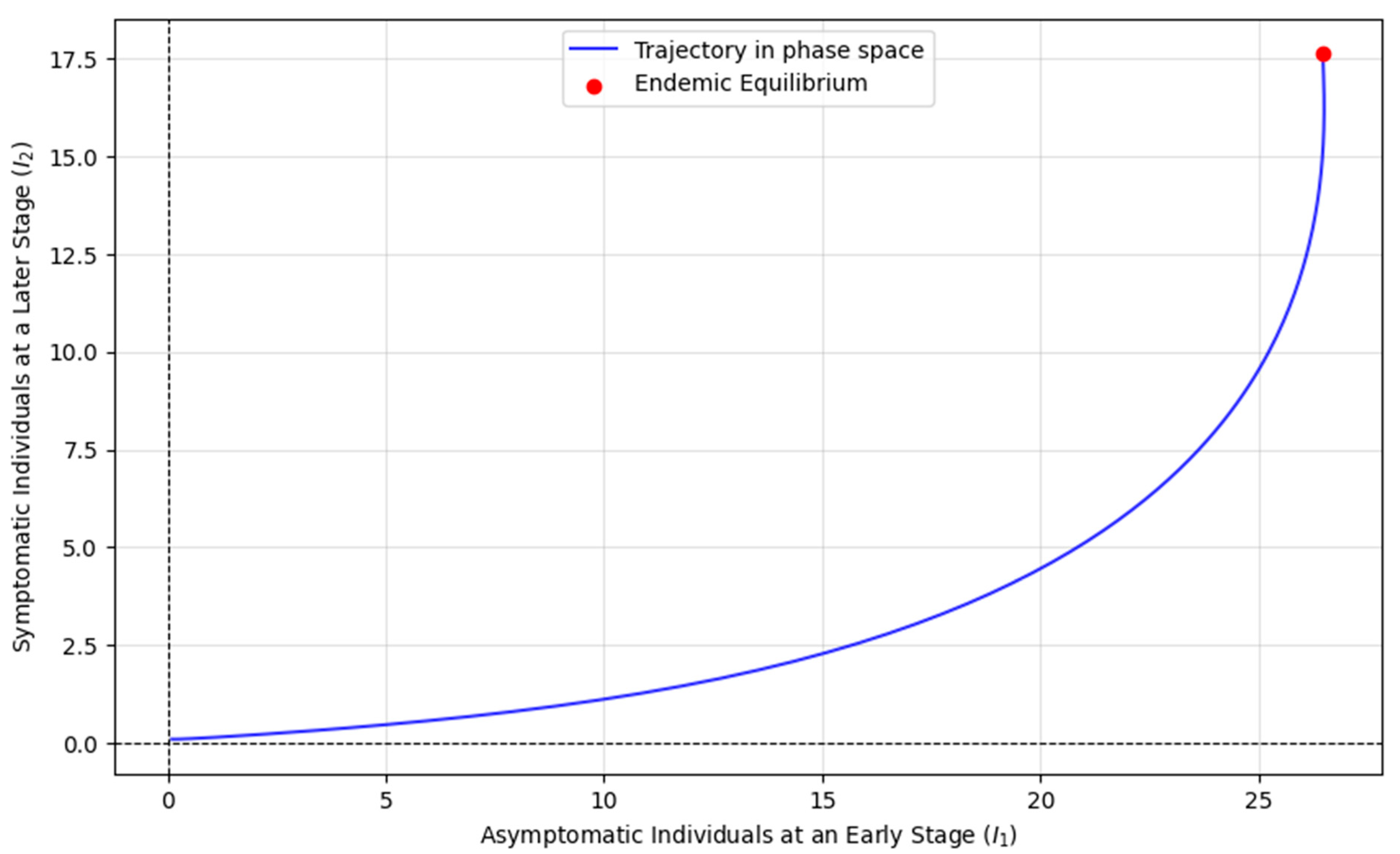
4.4. Endemic Equilibrium

The transition rate from susceptible to infectious agents, represented as η = β$\left(i_1+i_2\right)$, is the force of infection, where β is a non-linear communicable parameter. This nonlinearity is one of the critical capabilities of dynamic infectious disease models. Solving model at steady state gives the following:

$${\displaystyle \frac{\mathrm{d}\mathrm{S}}{\mathrm{d}\mathrm{t}}}=\mathrm{b}-\beta \mathrm{s}\left({\mathrm{I}}_1+{\mathrm{I}}_2\right)-\mu \mathrm{S}$$

$${\displaystyle \frac{\mathrm{d}\mathrm{E}}{\mathrm{d}\mathrm{t}}}=\beta \mathrm{S}\left({\mathrm{I}}_1+{\mathrm{I}}_2\right)-\lambda \mathrm{E}-\mu \mathrm{E}$$

$${\displaystyle \frac{\mathrm{d}{\mathrm{I}}_1}{\mathrm{d}\mathrm{t}}}=\lambda \mathrm{E}-\gamma {\mathrm{I}}_1-{\epsilon }_1{\mathrm{I}}_1-\mu {\mathrm{I}}_1$$

$${\displaystyle \frac{\mathrm{d}{\mathrm{I}}_2}{\mathrm{d}\mathrm{t}}}={\gamma \mathrm{I}}_1-{\epsilon }_1{\mathrm{I}}_2-\mu {\mathrm{I}}_2$$

$${\displaystyle \frac{\mathrm{d}\mathrm{R}}{\mathrm{d}\mathrm{t}}}={\epsilon }_1{\mathrm{I}}_1+{\epsilon }_1{\mathrm{I}}_2-\mu \mathrm{R}$$

Solving the model at steady state

$${\mathrm{S}}^{\mathrm{*}\mathrm{*}}={\displaystyle \frac{\mathrm{b}}{{\eta }^{\mathrm{*}\mathrm{*}}+\mu }},; {\mathrm{E}}^{\mathrm{*}\mathrm{*}}={\displaystyle \frac{{\eta }^{\mathrm{*}\mathrm{*}}\mathrm{b}}{({\eta }^{\mathrm{*}\mathrm{*}}+\mu )(\lambda +\mu )}}; {{\mathrm{I}}_1}^{\mathrm{*}\mathrm{*}}={\displaystyle \frac{\lambda {\eta }^{\mathrm{*}\mathrm{*}}\mathrm{b}}{(\gamma +{\epsilon }_1+\mu )({\eta }^{\mathrm{*}\mathrm{*}}+\mu )(\lambda +\mu )}};$$

$${{\mathrm{I}}_2}^{\mathrm{*}\mathrm{*}}={\displaystyle \frac{\gamma \lambda {\eta }^{\mathrm{*}\mathrm{*}}\mathrm{b}}{({\epsilon }_1+\mu )(\gamma +{\epsilon }_1+\mu )({\eta }^{\mathrm{*}\mathrm{*}}+\mu )(\lambda +\mu )}}; {\mathrm{R}}^{\mathrm{*}\mathrm{*}}={\displaystyle \frac{{\epsilon }_1{(\mathrm{i}}_1+{\mathrm{i}}_2)\gamma \lambda {\eta }^{\mathrm{*}\mathrm{*}}\mathrm{b}}{({\epsilon }_1+\mu )(\gamma +{\epsilon }_1+\mu )({\eta }^{\mathrm{*}\mathrm{*}}+\mu )(\lambda +\mu )}};$$

$${\mathrm{P}}_1=(\lambda +\mu ); {\mathrm{P}}_2=(\gamma +{\epsilon }_1+\mu ); {\mathrm{P}}_3=({\epsilon }_1+\mu )$$

$${\mathrm{S}}^{\mathrm{*}\mathrm{*}}={\displaystyle \frac{\mathrm{b}}{{\eta }^{\mathrm{*}\mathrm{*}}+\mu }}; {\mathrm{E}}^{\mathrm{*}\mathrm{*}}={\displaystyle \frac{{\eta }^{\mathrm{*}\mathrm{*}}\mathrm{b}}{({\eta }^{\mathrm{*}\mathrm{*}}+\mu ){\mathrm{P}}_1}}; {{\mathrm{I}}_1}^{\mathrm{*}\mathrm{*}}={\displaystyle \frac{\lambda {\eta }^{\mathrm{*}\mathrm{*}}\mathrm{b}}{{{\mathrm{P}}_1\mathrm{P}}_2({\eta }^{\mathrm{*}\mathrm{*}}+\mu )}};$$

$${{\mathrm{I}}_2}^{\mathrm{*}\mathrm{*}}={\displaystyle \frac{\gamma \lambda {\eta }^{\mathrm{*}\mathrm{*}}\mathrm{b}}{{{\mathrm{P}}_1{\mathrm{P}}_2\mathrm{P}}_3({\eta }^{\mathrm{*}\mathrm{*}}+\mu )}}; {\mathrm{R}}^{\mathrm{*}\mathrm{*}}={\displaystyle \frac{{\epsilon }_1}{\mu }}\left\{{\displaystyle \frac{\lambda {\eta }^{\mathrm{*}\mathrm{*}}\mathrm{b}}{{{\mathrm{P}}_1\mathrm{P}}_2({\eta }^{\mathrm{*}\mathrm{*}}+\mu )}}+{\displaystyle \frac{\gamma \lambda {\eta }^{\mathrm{*}\mathrm{*}}\mathrm{b}}{{{\mathrm{P}}_1{\mathrm{P}}_2\mathrm{P}}_3({\eta }^{\mathrm{*}\mathrm{*}}+\mu )}}\right\};$$

Now

$$\eta **=\beta \left({{\mathrm{I}}_1}^{\mathrm{*}\mathrm{*}}+{{\mathrm{I}}_2}^{\mathrm{*}\mathrm{*}}\right)$$

$$\eta **=\beta \left({\displaystyle \frac{\lambda {\eta }^{\mathrm{*}\mathrm{*}}\mathrm{b}}{{{\mathrm{P}}_1\mathrm{P}}_2({\eta }^{\mathrm{*}\mathrm{*}}+\mu )}}+{\displaystyle \frac{\gamma \lambda {\eta }^{\mathrm{*}\mathrm{*}}\mathrm{b}}{{{\mathrm{P}}_1{\mathrm{P}}_2\mathrm{P}}_3({\eta }^{\mathrm{*}\mathrm{*}}+\mu )}}\right)[\mathrm{Substituting} \mathrm{the} \mathrm{value} \mathrm{of} {{\mathrm{I}}_1}^{\mathrm{*}\mathrm{*}}\mathrm{and} {{\mathrm{I}}_2}^{\mathrm{*}\mathrm{*}}]$$

Now simplifying

$$1=\beta \left({\displaystyle \frac{\lambda \mathrm{b}}{{{\mathrm{P}}_1\mathrm{P}}_2({\eta }^{\mathrm{*}\mathrm{*}}+\mu )}}+{\displaystyle \frac{\gamma \lambda \mathrm{b}}{{{\mathrm{P}}_1{\mathrm{P}}_2\mathrm{P}}_3({\eta }^{\mathrm{*}\mathrm{*}}+\mu )}}\right)$$

$$\mathrm{or}, 1=\beta \lambda \mathrm{b}\left({\displaystyle \frac{{\mathrm{P}}_3+\gamma }{{{\mathrm{P}}_1{\mathrm{P}}_2\mathrm{P}}_3({\eta }^{\mathrm{*}\mathrm{*}}+\mu )}}\right) \mathrm{or},$$

$$\mathrm{or}, {{\mathrm{P}}_1{\mathrm{P}}_2\mathrm{P}}_3{\eta }^{\mathrm{*}\mathrm{*}}+{{\mathrm{P}}_1{\mathrm{P}}_2\mathrm{P}}_3\mu =\beta \lambda \mathrm{b}\left({\mathrm{P}}_3+\gamma \right)$$

$$\mathrm{or}, {{\mathrm{P}}_1{\mathrm{P}}_2\mathrm{P}}_3{\eta }^{\mathrm{*}\mathrm{*}}=\beta \lambda \mathrm{b}\left({\mathrm{P}}_3+\gamma \right)-{{\mathrm{P}}_1{\mathrm{P}}_2\mathrm{P}}_3\mu$$

$$\mathrm{or}, {\eta }^{\mathrm{*}\mathrm{*}}={\displaystyle \frac{\beta \lambda \mathrm{b}\left({\mathrm{P}}_3+\gamma \right)}{{{\mathrm{P}}_1{\mathrm{P}}_2\mathrm{P}}_3}}-{\displaystyle \frac{{{\mathrm{P}}_1{\mathrm{P}}_2\mathrm{P}}_3\mu }{{{\mathrm{P}}_1{\mathrm{P}}_2\mathrm{P}}_3}}$$

$$\mathrm{or}, {\eta }^{\mathrm{*}\mathrm{*}}=\mu \left\{{\displaystyle \frac{\beta \lambda \mathrm{b}\left({\mathrm{P}}_3+\gamma \right)}{{{\mu \mathrm{P}}_1{\mathrm{P}}_2\mathrm{P}}_3}}-1\right\}$$

$$\mathrm{or}, {\eta }^{\mathrm{*}\mathrm{*}}=\mu \left\{{\displaystyle \frac{\beta \lambda \mathrm{b}}{{\mu \mathrm{P}}_1{\mathrm{P}}_2}}+{\displaystyle \frac{\beta \lambda \mathrm{b}\gamma }{{{\mu \mathrm{P}}_1{\mathrm{P}}_2\mathrm{P}}_3}}-1\right\}$$

$$\mathrm{or}, {\eta }^{\mathrm{*}\mathrm{*}}=\mu \left\{{\mathrm{R}}_0+{\displaystyle \frac{\beta \lambda \mathrm{b}\gamma }{{{\mu \mathrm{P}}_1{\mathrm{P}}_2\mathrm{P}}_3}}-1\right\}$$

$$\mathrm{or}, {\eta }^{\mathrm{*}\mathrm{*}}\le \mu \left\{{\mathrm{R}}_0-1\right\}$$

Since ${\eta }^{**}$ has a unique value in this case, ${\mathrm{R}}_0>1$ since it must be more significant than 1. If ${\mathrm{R}}_0>1$ and ${\mathrm{R}}_0<1$, respectively, then the Endemic equilibrium is locally asymptotically stable and unstable. As a result, we have a unique positive endemic equilibrium here.

Figure 4 illustrates the dynamics of two infectious stages, I₁ (asymptomatic people at an early stage) and I₂ (symptomatic people at a later stage), within a population exposed to an epidemic. The trajectories represent the changes in the sizes of these infectious groups over time as individuals transition between susceptible, exposed, and contagious states. The red dot marks the endemic equilibrium, where the number of individuals in both infectious stages stabilizes, meaning that the disease persists steadily in the population. This equilibrium occurs when the basic reproduction number R₀ > 1, implying that each infected individual is transmitting the disease to more than one person, leading to ongoing transmission. In the context of the model, the primary infectious individuals (I₁) represent those actively spreading the disease. In contrast, the secondary infectious (I₂) may have progressed to a more severe stage, further contributing to disease spread. The stability of this endemic equilibrium suggests that the disease will continue circulating in the population, with both i₁ and i₂ reaching steady-state values. The biological and epidemiological significance lies in the understanding that, once an epidemic surpasses a certain threshold of transmissibility (R₀ > 1), the disease cannot be eradicated and will persist in the population unless control measures intervene.

4.5. Stability Analysis at Equilibrium Point and Hopf-Bifurcation

In this case, we consider the incubation time τ > 0, during which the infected person became infectious. Susceptible s(t), exposed e(t), asymptomatic people at an early stage i₁(t), and symptomatic people at a later stage i₂(t) are the state variables. Models are created using

$${\displaystyle \frac{\mathrm{d}\mathrm{S}}{\mathrm{d}\mathrm{t}}}=\mathrm{b}-\beta \mathrm{S}{\mathrm{I}}_1\left(\mathrm{t}-\tau \right)-\beta \mathrm{S}{\mathrm{I}}_2\left(\mathrm{t}-\tau \right)-\mu \mathrm{S}$$

$${\displaystyle \frac{\mathrm{d}\mathrm{E}}{\mathrm{d}\mathrm{t}}}=\beta \mathrm{S}{\mathrm{I}}_1\left(\mathrm{t}-\tau \right)+\beta \mathrm{S}{\mathrm{I}}_2\left(\mathrm{t}-\tau \right)-\lambda \mathrm{E}-\mu \mathrm{E}$$

$${\displaystyle \frac{\mathrm{d}{\mathrm{I}}_1}{\mathrm{d}\mathrm{t}}}=\lambda \mathrm{E}\left(\mathrm{t}-\tau \right)-\gamma {\mathrm{I}}_1-{\epsilon }_1{\mathrm{I}}_1-\mu {\mathrm{I}}_1-{\tau }_1{\mathrm{I}}_1$$

$${\displaystyle \frac{\mathrm{d}{\mathrm{I}}_2}{\mathrm{d}\mathrm{t}}}={\gamma \mathrm{I}}_1-\psi {\mathrm{I}}_2-{\epsilon }_1{\mathrm{I}}_2-\mu {\mathrm{I}}_2-{\tau }_2{\mathrm{I}}_2$$

where S(0) > 0, E(0) > 0, I₁ > 0, I₂ > 0 with an initial history function for I₁ and I₂ specified over t ∈ [−τ, 0].

All parameters are considered positive constants.

At the equilibrium point, ${\displaystyle \frac{dS}{dt}}=0$, ${\displaystyle \frac{dE}{dt}}=0$, ${\displaystyle \frac{d{I}_1}{dt}}=0, {\displaystyle \frac{d{I}_2}{dt}}=0$ and considering S*, E*, I₁*, I₂* denote the steady state values. The force of infection is defined as follows:

$$\eta =\beta ({\mathrm{I}}_1^{\mathrm{*}}+{\mathrm{I}}_2^{\mathrm{*}})\mathrm{where}\beta \mathrm{is}\mathrm{a}\mathrm{non-linear}\mathrm{communicable}\mathrm{parameter}.$$

$${\displaystyle \frac{\mathrm{d}{\mathrm{S}}^{\mathrm{*}}}{\mathrm{d}\mathrm{t}}}=0=> {\mathrm{S}}^{\mathrm{*}}={\displaystyle \frac{\mathrm{b}}{\eta +\mu };}$$

$${\displaystyle \frac{\mathrm{d}{\mathrm{E}}^{\mathrm{*}}}{\mathrm{d}\mathrm{t}}}=0=> {\mathrm{E}}^{\mathrm{*}}={\displaystyle \frac{{\eta }^{\mathrm{*}}\mathrm{b}}{(\eta +\mu )(\lambda +\mu )}};$$

$${\displaystyle \frac{\mathrm{d}{{\mathrm{I}}_1}^{\mathrm{*}}}{\mathrm{d}\mathrm{t}}}=0=> {{\mathrm{I}}_1}^{\mathrm{*}}={\displaystyle \frac{\lambda \eta \mathrm{b}}{(\gamma +{\epsilon }_1+\mu )(\eta +\mu )(\lambda +\mu )}};$$

$${\displaystyle \frac{\mathrm{d}{{\mathrm{I}}_2}^{\mathrm{*}}}{\mathrm{d}\mathrm{t}}}=0=> {{\mathrm{I}}_2}^{\mathrm{*}}={\displaystyle \frac{\gamma \lambda \eta \mathrm{b}}{({\epsilon }_1+\mu )(\gamma +{\epsilon }_1+\mu )(\eta +\mu )(\lambda +\mu )}};$$

$${\mathrm{P}}_1=(\lambda +\mu ); {\mathrm{P}}_2=(\gamma +{\epsilon }_1+\mu ); {\mathrm{P}}_3=({\epsilon }_1+\mu )$$

$${\mathrm{S}}^{\mathrm{*}}={\displaystyle \frac{\mathrm{b}}{\eta +\mu }}; {\mathrm{E}}^{\mathrm{*}}={\displaystyle \frac{\eta \mathrm{b}}{(\eta +\mu ){\mathrm{P}}_1}}; {{\mathrm{I}}_1}^{\mathrm{*}}={\displaystyle \frac{\lambda \eta \mathrm{b}}{{{\mathrm{P}}_1\mathrm{P}}_2(\eta +\mu )}};{{\mathrm{I}}_2}^{\mathrm{*}}={\displaystyle \frac{\gamma \lambda \eta \mathrm{b}}{{{\mathrm{P}}_1{\mathrm{P}}_2\mathrm{P}}_3(\eta +\mu )}};$$

$${\mathrm{E}}^{*} \left({\displaystyle \frac{\mathrm{b}}{\eta +\mu }},{\displaystyle \frac{\eta \mathrm{b}}{(\eta +\mu ){\mathrm{P}}_1}},{\displaystyle \frac{\lambda \eta \mathrm{b}}{{{\mathrm{P}}_1\mathrm{P}}_2(\eta +\mu )}},{\displaystyle \frac{\gamma \lambda \eta \mathrm{b}}{{{\mathrm{P}}_1{\mathrm{P}}_2\mathrm{P}}_3(\eta +\mu )}}\right)$$

At the equilibrium point the equations become

$${\displaystyle \frac{\mathrm{d}{\mathrm{S}}^{\mathrm{*}}}{\mathrm{d}\mathrm{t}}}=\mathrm{b}-\beta {\mathrm{S}}^{\mathrm{*}}{\mathrm{I}}_1^{\mathrm{*}}\left(\mathrm{t}-\tau \right)-\beta {\mathrm{S}}^{\mathrm{*}}{\mathrm{I}}_2^{\mathrm{*}}\left(\mathrm{t}-\tau \right)-\mu {\mathrm{S}}^{\mathrm{*}}$$

$${\displaystyle \frac{\mathrm{d}{\mathrm{E}}^{\mathrm{*}}}{\mathrm{d}\mathrm{t}}}=\beta {\mathrm{S}}^{\mathrm{*}}{\mathrm{I}}_1^{\mathrm{*}}\left(\mathrm{t}-\tau \right)+\beta {\mathrm{S}}^{\mathrm{*}}{\mathrm{I}}_2^{\mathrm{*}}\left(\mathrm{t}-\tau \right)-\lambda {\mathrm{E}}^{\mathrm{*}}-\mu {\mathrm{E}}^{\mathrm{*}}$$

$${\displaystyle \frac{\mathrm{d}{\mathrm{I}}_1}{\mathrm{d}\mathrm{t}}}=\lambda {\mathrm{E}}^{\mathrm{*}}\left(\mathrm{t}-\tau \right)-\gamma {\mathrm{I}}_1^{\mathrm{*}}-{\epsilon }_1{\mathrm{I}}_1^{\mathrm{*}}-\mu {\mathrm{I}}_1^{\mathrm{*}}-{\tau }_1{\mathrm{I}}_1^{\mathrm{*}}$$

$${\displaystyle \frac{\mathrm{d}{\mathrm{I}}_2}{\mathrm{d}\mathrm{t}}}=\gamma {\mathrm{I}}_1^{\mathrm{*}}-\psi {\mathrm{I}}_2^{\mathrm{*}}-{\epsilon }_1{\mathrm{I}}_2^{\mathrm{*}}-\mu {\mathrm{I}}_2^{\mathrm{*}}-{\tau }_2{\mathrm{I}}_2^{\mathrm{*}}$$

Let $\mathrm{f}\left({\mathrm{S}}^{\mathrm{*}},{\mathrm{E}}^{\mathrm{*}},{\mathrm{I}}_1^{\mathrm{*}},{\mathrm{I}}_2^{\mathrm{*}}\right)=\mathrm{b}-\beta {\mathrm{S}}^{\mathrm{*}}{\mathrm{I}}_1^{\mathrm{*}}\left(\mathrm{t}-\tau \right)-\beta {\mathrm{S}}^{\mathrm{*}}{\mathrm{I}}_2^{\mathrm{*}}\left(\mathrm{t}-\tau \right)-\mu {\mathrm{S}}^{\mathrm{*}}$

$$\mathrm{g}\left({\mathrm{S}}^{\mathrm{*}},{\mathrm{E}}^{\mathrm{*}},{\mathrm{I}}_1^{\mathrm{*}},{\mathrm{I}}_2^{\mathrm{*}}\right)=\beta {\mathrm{S}}^{\mathrm{*}}{\mathrm{I}}_1^{\mathrm{*}}\left(\mathrm{t}-\tau \right)+\beta {\mathrm{S}}^{\mathrm{*}}{\mathrm{I}}_2^{\mathrm{*}}\left(\mathrm{t}-\tau \right)-\lambda {\mathrm{E}}^{\mathrm{*}}-\mu {\mathrm{E}}^{\mathrm{*}}$$

$$\mathrm{h}\left({\mathrm{S}}^{\mathrm{*}},{\mathrm{E}}^{\mathrm{*}},{\mathrm{I}}_1^{\mathrm{*}},{\mathrm{I}}_2^{\mathrm{*}}\right)=\lambda {\mathrm{E}}^{\mathrm{*}}\left(\mathrm{t}-\tau \right)-\gamma {\mathrm{I}}_1^{\mathrm{*}}-{\epsilon }_1{\mathrm{I}}_1^{\mathrm{*}}-\mu {\mathrm{I}}_1^{\mathrm{*}}-{\tau }_1{\mathrm{I}}_1^{\mathrm{*}}$$

$$\mathrm{k}\left({\mathrm{S}}^{\mathrm{*}},{\mathrm{E}}^{\mathrm{*}},{\mathrm{I}}_1^{\mathrm{*}},{\mathrm{I}}_2^{\mathrm{*}}\right)=\gamma {\mathrm{I}}_1^{\mathrm{*}}-\psi {\mathrm{I}}_2^{\mathrm{*}}-{\epsilon }_1{\mathrm{I}}_2^{\mathrm{*}}-\mu {\mathrm{I}}_2^{\mathrm{*}}-{\tau }_2{\mathrm{I}}_2^{\mathrm{*}}$$

Now J $\left({\mathrm{S}}^{\mathrm{*}},{\mathrm{E}}^{\mathrm{*}},{\mathrm{I}}_1^{\mathrm{*}},{\mathrm{I}}_2^{\mathrm{*}}\right)$ = $\left(\begin{array}{cccc}{\displaystyle \frac{𝜕\mathrm{f}}{𝜕\mathrm{S}}}& {\displaystyle \frac{𝜕\mathrm{f}}{𝜕\mathrm{E}}}& {\displaystyle \frac{𝜕\mathrm{f}}{𝜕{\mathrm{I}}_1}}& {\displaystyle \frac{𝜕\mathrm{f}}{𝜕{\mathrm{I}}_2}}\\ {\displaystyle \frac{𝜕\mathrm{g}}{𝜕\mathrm{S}}}& {\displaystyle \frac{𝜕\mathrm{g}}{𝜕\mathrm{E}}}& {\displaystyle \frac{𝜕\mathrm{g}}{𝜕{\mathrm{I}}_1}}& {\displaystyle \frac{𝜕\mathrm{g}}{𝜕{\mathrm{I}}_2}}\\ {\displaystyle \frac{𝜕\mathrm{h}}{𝜕\mathrm{S}}}& {\displaystyle \frac{𝜕\mathrm{h}}{𝜕\mathrm{E}}}& {\displaystyle \frac{𝜕\mathrm{h}}{𝜕{\mathrm{I}}_1}}& {\displaystyle \frac{𝜕\mathrm{h}}{𝜕{\mathrm{I}}_2}}\\ {\displaystyle \frac{𝜕\mathrm{k}}{𝜕\mathrm{S}}}& {\displaystyle \frac{𝜕\mathrm{k}}{𝜕\mathrm{E}}}& {\displaystyle \frac{𝜕\mathrm{k}}{𝜕{\mathrm{I}}_1}}& {\displaystyle \frac{𝜕\mathrm{k}}{𝜕{\mathrm{I}}_2}}\end{array}\right)$

$$=\left(\begin{array}{cccc}-\eta -\mu & 0& -\beta \mathrm{S}{\mathrm{e}}^{-\lambda \tau }& -\beta \mathrm{S}{\mathrm{e}}^{-\lambda \tau }\\ \eta & -\lambda -\mu & 0& 0\\ 0& \lambda {\mathrm{e}}^{-\lambda \tau }& -\gamma -{\epsilon }_1-\mu & 0\\ 0& 0& \gamma & -\psi -{\epsilon }_1-\mu \end{array}\right)$$

$$(\mathrm{J}\left({\mathrm{S}}^{\mathrm{*}},{\mathrm{E}}^{\mathrm{*}},{\mathrm{I}}_1^{\mathrm{*}},{\mathrm{I}}_2^{\mathrm{*}}\right)-{\lambda }_1\mathrm{I})=\left(\begin{array}{cccc}-\eta -\mu -{\lambda }_1& 0& -\beta \mathrm{S}{\mathrm{e}}^{-\lambda \tau }-{\lambda }_1& -\beta \mathrm{S}{\mathrm{e}}^{-\lambda \tau }-{\lambda }_1\\ \eta -{\lambda }_1& -\lambda -\mu -{\lambda }_1& 0& 0\\ 0& \lambda {\mathrm{e}}^{-\lambda \tau }-{\lambda }_1& -\gamma -{\epsilon }_1-\mu -{\lambda }_1& 0\\ 0& 0& \gamma -{\lambda }_1& -\psi -{\epsilon }_1-\mu -{\lambda }_1\end{array}\right)$$

$$\begin{gathered} \det |\mathrm{J}\left({\mathrm{S}}^{\mathrm{*}},{\mathrm{E}}^{\mathrm{*}},{\mathrm{I}}_1^{\mathrm{*}},{\mathrm{I}}_2^{\mathrm{*}}\right)-{\lambda }_1\mathrm{I}|=(-\eta -\mu -{\lambda }_1)(-\lambda -\mu -{\lambda }_1\left)\right(-\gamma -{\epsilon }_1-\mu -{\lambda }_1\left)\right(-\psi -{\epsilon }_1-\mu -{\lambda }_1) \\ =(\eta +\mu +{\lambda }_1)(\lambda +\mu +{\lambda }_1\left)\right(\gamma +{\epsilon }_1+\mu +{\lambda }_1\left)\right( \psi +{\epsilon }_1+\mu +{\lambda }_1 \end{gathered}$$

Here

$$\begin{array}{c}(\eta +\mu +{\lambda }_1)(\lambda +\mu +{\lambda }_1\left)\right(\gamma +{\epsilon }_1+\mu +{\lambda }_1\left)\right(\psi +{\epsilon }_1+\mu +{\lambda }_1)=0\hfill \\ {\mathrm{P}}_1=(\lambda +\mu ); {\mathrm{P}}_2=(\gamma +{\epsilon }_1+\mu ); {\mathrm{P}}_3=({\psi +\epsilon }_1+\mu )\hfill \end{array}$$

So,

$$\begin{gathered} (\eta +\mu +{\lambda }_1)({\mathrm{P}}_1+{\lambda }_1\left)\right({\mathrm{P}}_2+{\lambda }_1\left)\right({\mathrm{P}}_3+{\lambda }_1=0 \\ \Rightarrow {\lambda }_1^4+({\mathrm{P}}_3+{\mathrm{P}}_2+{\mathrm{P}}_1+\mu +\eta ){\lambda }_1^3+\left({\mathrm{P}}_2{\mathrm{P}}_3+{\mathrm{P}}_1{\mathrm{P}}_3+{\mathrm{P}}_1{\mathrm{P}}_2+\mu {\mathrm{P}}_3+\mu {\mathrm{P}}_2+\mu {\mathrm{P}}_1+\eta {\mathrm{P}}_3+\eta {\mathrm{P}}_2+\eta {\mathrm{P}}_1\right){\lambda }_1^2+\left({\mathrm{P}}_1{\mathrm{P}}_2{\mathrm{P}}_3+\mu {\mathrm{P}}_1{\mathrm{P}}_2+ \\ \mu {\mathrm{P}}_1{\mathrm{P}}_3+\mu {\mathrm{P}}_2{\mathrm{P}}_3+\eta {\mathrm{P}}_1{\mathrm{P}}_2+\eta {\mathrm{P}}_1{\mathrm{P}}_3+\eta {\mathrm{P}}_2{\mathrm{P}}_3\right){\lambda }_1+\eta {\mathrm{P}}_1{\mathrm{P}}_2{\mathrm{P}}_3+\mu {\mathrm{P}}_1{\mathrm{P}}_2{\mathrm{P}}_3=0 \end{gathered}$$

Considering

$$\mathrm{a}=({\mathrm{P}}_3+{\mathrm{P}}_2+{\mathrm{P}}_1+\mu +\eta );$$

$$\mathrm{b}=\left({\mathrm{P}}_2{\mathrm{P}}_3+{\mathrm{P}}_1{\mathrm{P}}_3+{\mathrm{P}}_1{\mathrm{P}}_2+\mu {\mathrm{P}}_3+\mu {\mathrm{P}}_2+\mu {\mathrm{P}}_1+\eta {\mathrm{P}}_3+\eta {\mathrm{P}}_2+\eta {\mathrm{P}}_1\right)$$

$$\mathrm{c}=\left({\mathrm{P}}_1{\mathrm{P}}_2{\mathrm{P}}_3+\mu {\mathrm{P}}_1{\mathrm{P}}_2+\mu {\mathrm{P}}_1{\mathrm{P}}_3+\mu {\mathrm{P}}_2{\mathrm{P}}_3+\eta {\mathrm{P}}_1{\mathrm{P}}_2+\eta {\mathrm{P}}_1{\mathrm{P}}_3+\eta {\mathrm{P}}_2{\mathrm{P}}_3\right)$$

$$\mathrm{d}=\eta {\mathrm{P}}_1{\mathrm{P}}_2{\mathrm{P}}_3+\mu {\mathrm{P}}_1{\mathrm{P}}_2{\mathrm{P}}_3$$

$${\lambda }_1^4+\mathrm{a}{\lambda }_1^3+\mathrm{b}{\lambda }_1^2+\mathrm{c}{\lambda }_1+\mathrm{d}+\mathrm{f}{\mathrm{e}}^{-\lambda \tau }=0$$

where ${fe}^{-\lambda \tau }$ represents the delayed terms. The delay $\tau$ can affect stability by shifting eigenvalues into the right-half complex plane.

Here, for a small $\tau$, stability is determined using Routh–Hurwitz criteria and for a large $\tau$, the delay can introduce Hopf bifurcation, leading to oscillations.

Applying the D-matrix Approach if all the roots of the delay-free characteristics equation ${\lambda }_1^4+\mathrm{a}{\lambda }_1^3$ + $\mathrm{b}{\lambda }_1^2+\mathrm{c}{\lambda }_1+\mathrm{d}=0$ has a negative real part, and the system is locally asymptotically stable.

To analyze the Routh–Hurwitz criterion, we construct the Routh array included in

Table 1. Routh array.

Row	${\mathsf{\lambda }}^4$	${\mathsf{\lambda }}^3$	${\mathsf{\lambda }}^2$	${\mathsf{\lambda }}^1$	${\mathsf{\lambda }}^0$
1	1	b	d	0
2	a	c	0	0
3	${\displaystyle \frac{\mathrm{a}\mathrm{b}-\mathrm{c}}{\mathrm{a}}}$	${\displaystyle \frac{\mathrm{a}\mathrm{d}}{\mathrm{a}}}-\mathrm{d}$	0	0
4	${\displaystyle \frac{\mathrm{c}\mathrm{d}-\mathrm{a}\mathrm{b}\mathrm{d}}{\mathrm{c}}}$	0	0	0

and check the necessary condition

The system will be stable when all elements in the first column of the Routh array must be positive. Which leads to the following condition:

a > 0, b > 0, c > 0, d > 0, ab − c > 0 and cd − abd > 0 if all o these conditions are satisfied, then

All the roots of the characteristic equation will have negative real parts, ensuring that the system is locally asymptotically stable. Otherwise, the system has at least one eigenvalue with a nonnegative real part, which could lead to instability or marginal stability.

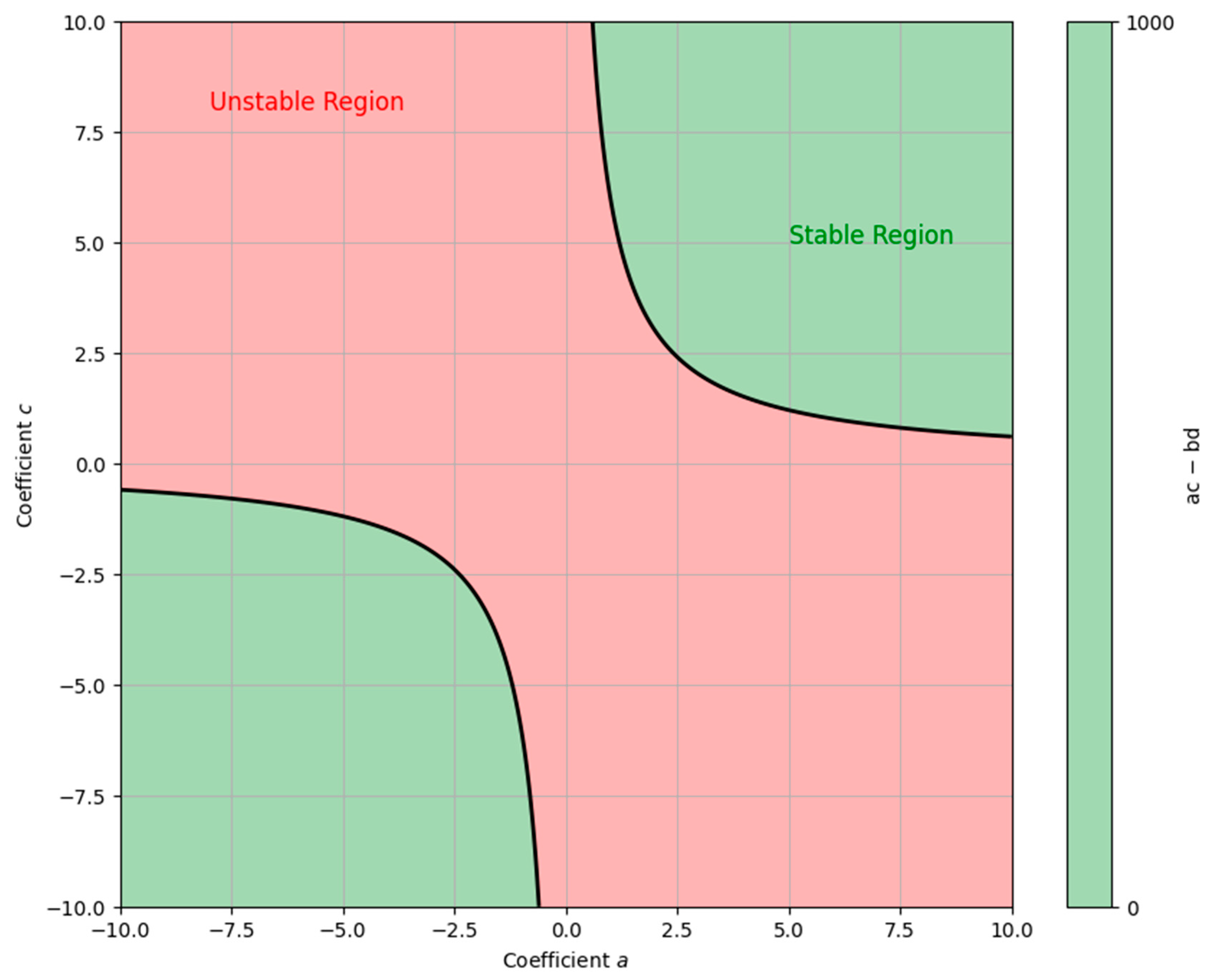
Figure 5 illustrates a system’s stability and instability regions described by a 4th-degree polynomial using the Routh–Hurwitz criterion. The X-axis and Y-axis represent the coefficients a and c of the polynomial, while b and d are constants. The green area shows where the system is stable (ac − bd > 0), meaning perturbations will decay over time. The red area represents instability (ac − bd < 0), where perturbations grow, leading to instability. The black line marks the boundary between these regions, indicating that the system is on the verge of instability.

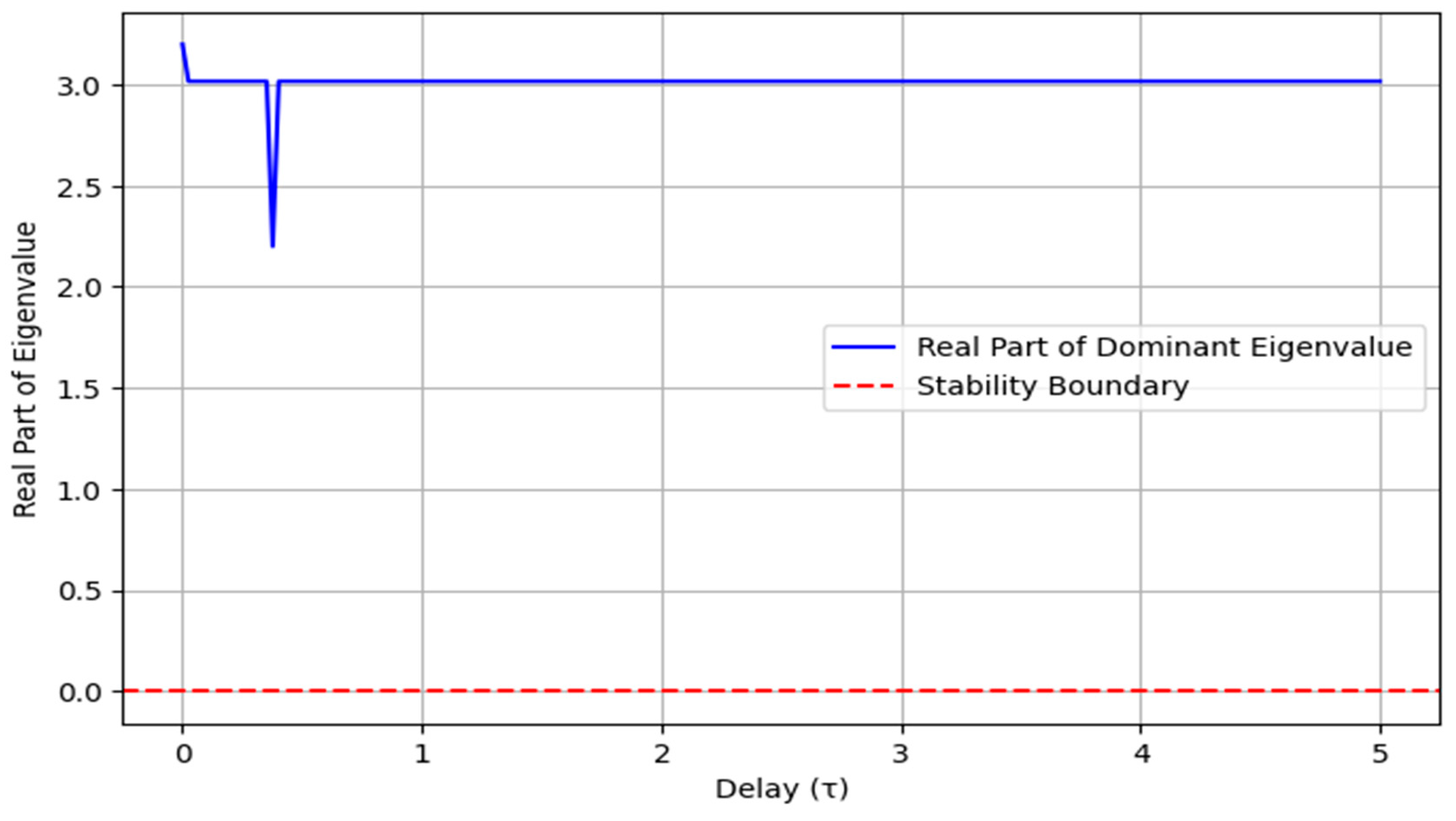
Figure 6 illustrates how the real part of the dominant eigenvalue varies with the delay parameter (τ). Initially, for small values of τ, the real part of the eigenvalue remains negative, indicating a stable system. However, as τ increases, the eigenvalue approaches zero and eventually becomes positive, marking a transition to instability. The red dashed line represents the stability boundary at λ = 0, beyond which the system loses stability. This suggests that increasing the delay can destabilize the system, emphasizing the importance of controlling delay in dynamic systems to maintain stability.

5. Data Fitting and Numerical Analysis

This prospective study [32] examined HSV transmission dynamics in 214 initially enrolled couples, of which 144 heterosexual couples were included in the analysis. In these pairs, the source partner experienced recurrent genital HSV, while the susceptible partner had no prior evidence of infection. Over a median follow-up period of 334 days, HSV transmission occurred in 14 couples (9.7%). Women without antibodies to HSV-1 or HSV-2 faced a significantly higher transmission risk (31.8%) than those with HSV-1 antibodies (9.1%). Couples who successfully avoided transmission reported fewer symptomatic episodes in source partners. Notably, most transmissions (9 out of 13) occurred during asymptomatic periods, while the remainder were associated with prodromal symptoms or the early stages of lesion development.

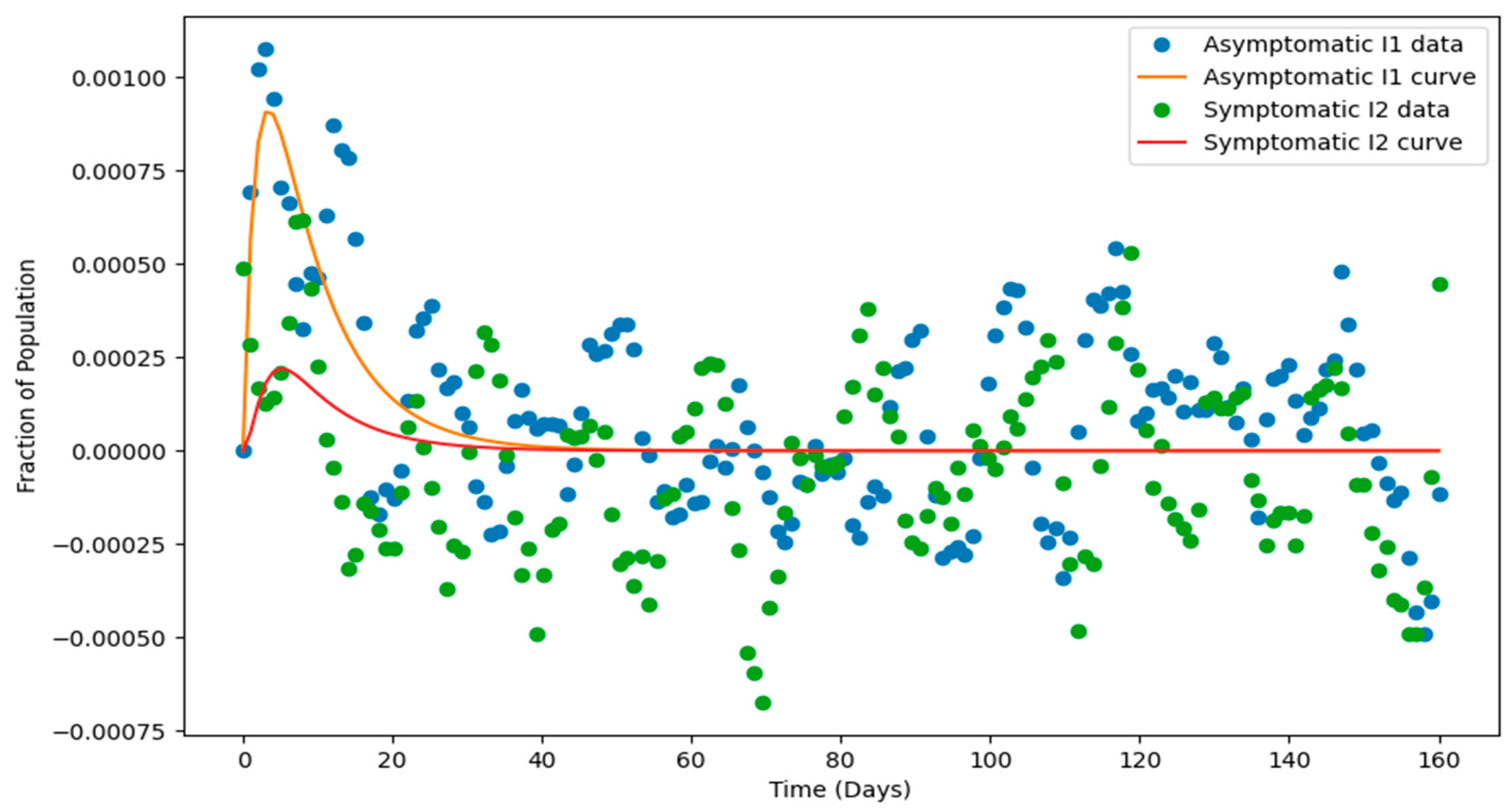
Without real data and reference values, we make assumptions about realistic parameter values based on previous studies [33,34]. We use smoothed noisy data to demonstrate the model’s applicability and validate its dynamics. The diagram illustrates the dynamics of two infected compartments, ${\mathrm{I}}_1$and ${\mathrm{I}}_2$, within a compartmental epidemiological model, showcasing both the smoothed noisy data (circles) and the fitted model curves (solid lines). The smoothed data, derived using the Savitzky-Golay filter, highlights the underlying trends by minimizing random noise while preserving the general pattern.

The fitted curve Figure 7, obtained through parameter estimation via curve fitting, aligns closely with the smoothed data, demonstrating the model’s ability to capture the infection dynamics. The trajectories reveal a rapid rise in ${\mathrm{I}}_1$ as the infection spreads, followed by a delayed rise in the ${\mathrm{I}}_2$, reflecting a sequential progression between the compartments. Both compartments eventually decline as recovery or control measures reduce infection levels. The peaks in ${\mathrm{I}}_1$ and ${\mathrm{I}}_2$ represent critical moments in the epidemic’s progression, while the delay between their peaks suggests transitions between stages of infection. Overall, the diagram underscores the model’s effectiveness in describing the infection dynamics and its potential utility in understanding and predicting epidemic behavior.

The parameters outlined in

Table 2. The parameter values for the model are specified, considering a total population (N) of 100,000 when the basic reproduction number (R₀) is set to 1.7045, indicating a value greater than 1.

S/N	Parameter	Description	Values	Source
1	b	Birth rate	0.00014 day−1	Estimated
2	$\beta$	Transmission rate	0.0001 day−1	Estimated
3	$\mu$	The inherent mortality rate	0.05 day−1	Estimated
4	$\lambda$	The rate at which individuals transition from the exposed class to the asymptomatic class	0.06 day−1	Fitted [5,32,33,34]
5	$\gamma$	The transition rate from the asymptomatic to the symptomatic class	0.1 day−1	Fitted [5,32,33,34]
6	${\epsilon }_1$	The inherent rate of recovery for individuals in the asymptomatic class.	0.03 day−1	Fitted [5,32,33,34]
7	${\tau }_1$	Rate of antiviral treatment for asymptomatic	0.25 day−1	Fitted [5,32,33,34]
8	$\psi$	Progression rate to treatment class under mechanical ventilation	0.02 day−1	Fitted [5,32,33,34]
9	${\tau }_2$	Treatment rate with antiviral medication for individuals exhibiting symptoms	0.75 day−1	Fitted [5,32,33,34]
10	$\sigma$	Rate of progression in ICU treatment	0.04 day−1	Fitted [5,32,33,34]
11	${\phi }_v$	Rate of recovery as a result of treatment in ventilation	0.045 day−1	Fitted [5,32,33,34]
12	$\delta$	Mortality rate attributed to the disease	0.02 day−1	Fitted [5,32,33,34]
13	$\alpha$	Rate of progressed to treatment class under Recovery People	0.002 day−1	Fitted [5,32,33,34]
14	${\phi }_i$	Rate of recovery as a result of ICU treatment	0.04 day−1	Fitted [5,32,33,34]
15	$\theta$	Factor adjusting the progression to death among treated individuals	0.25 day−1	Fitted [5,32,33,34]

and

Table 3. Values of the different parameters of the model with total population N = 100,000 when R₀ = 0.9703 < 1.

S/N	Parameter	Description	Values	Source
1	b	Birth rate	0.00014 day−1	Estimated
2	$\beta$	Transmission rate	0.000005 day−1	Estimated
3	$\mu$	The inherent mortality rate	0.4 day−1	Estimated
4	$\lambda$	The rate at which individuals transition from the exposed class to the asymptomatic class	0.1 day−1	Fitted [5,32,33,34]
5	$\gamma$	The transition rate from the asymptomatic to the symptomatic class	0.4 day−1	Fitted [5,32,33,34]
6	${\epsilon }_1$	The inherent rate of recovery for individuals in the asymptomatic class.	0.001 day−1	Fitted [5,32,33,34]
7	${\tau }_1$	Rate of antiviral treatment for asymptomatic	0.0025 day−1	Fitted [5,32,33,34]
8	$\psi$	Progression rate to treatment class under mechanical ventilation	0.023 day−1	Fitted [5,32,33,34]
9	${\tau }_2$	Treatment rate with antiviral medication for individuals exhibiting symptoms	0.75 day−1	Fitted [5,32,33,34]
10	$\sigma$	Rate of progression in ICU treatment	0.03 day−1	Fitted [5,32,33,34]
11	${\phi }_v$	Rate of recovery as a result of treatment in ventilation	1.0045 day−1	Fitted [5,32,33,34]
12	$\delta$	Mortality rate attributed to the disease.	0.002 day−1	Fitted [5,32,33,34]
13	$\alpha$	Rate of progressed to treatment class under Recovery People	0.002 day−1	Fitted [5,32,33,34]
14	${\phi }_i$	Rate of recovery as a result of ICU treatment	0.0000075 day−1	Fitted [5,32,33,34]
15	$\theta$	Factor adjusting the progression to death among treated individuals	0.25 day−1	Fitted [5,32,33,34]

will be used for simulation. The values assigned to these parameters have been extracted from various literature sources [5,32,33,34]. This simulation aims to demonstrate specific theoretical findings derived from the study visually.

Here, in the models devoid of control, it is noted that the numerical simulation’s outcome demonstrates a direct correlation between the reproduction number and the rates of transmission $\beta$ and progression to treatment class $\psi$ under mechanical ventilation. The reproduction number rises when $\beta$ and $\psi$ rise, while the reproduction number falls when they fall. Brain encephalitis can be eliminated from the community provided that the rate of infection $\beta$ and the transmission partner decreases.

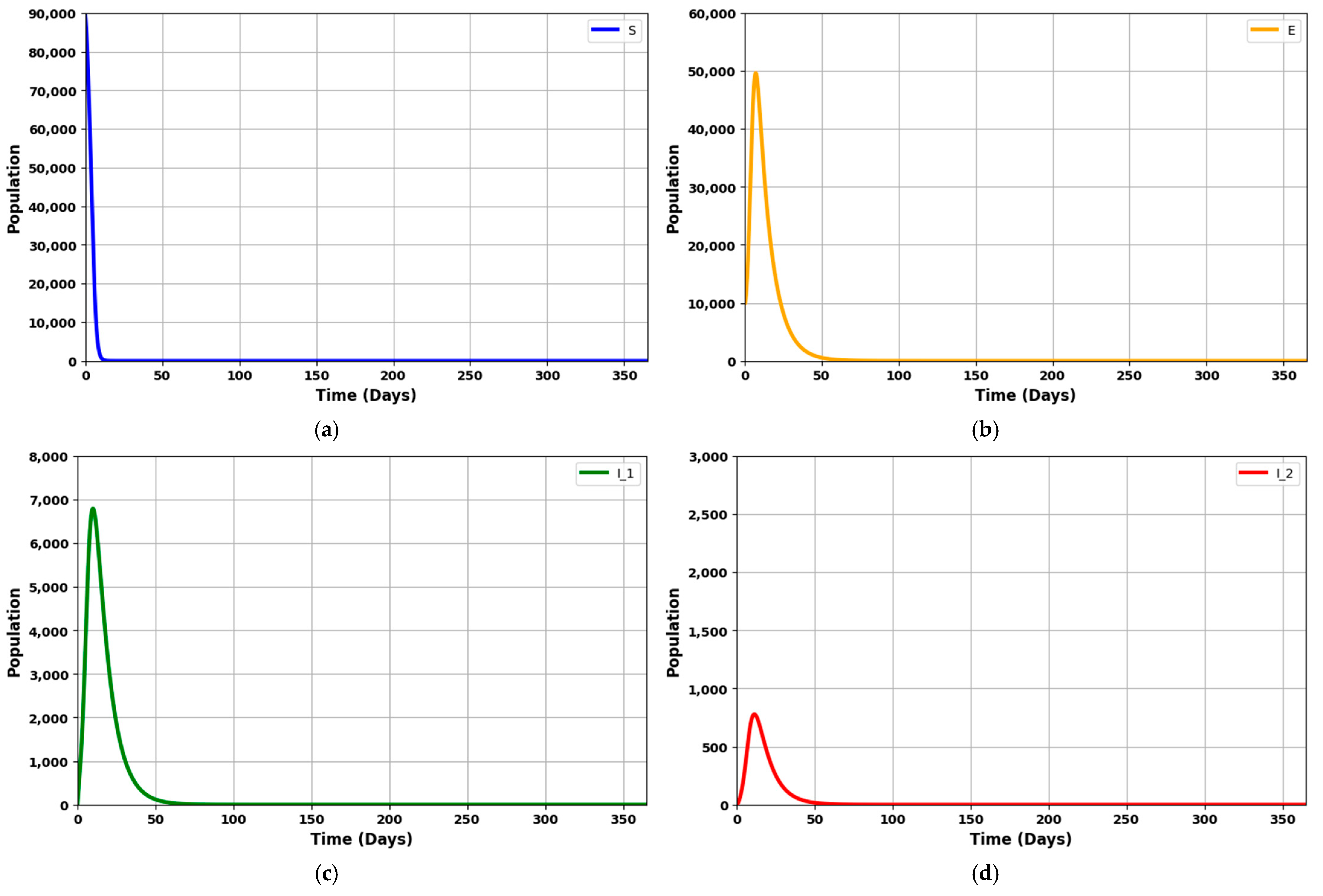
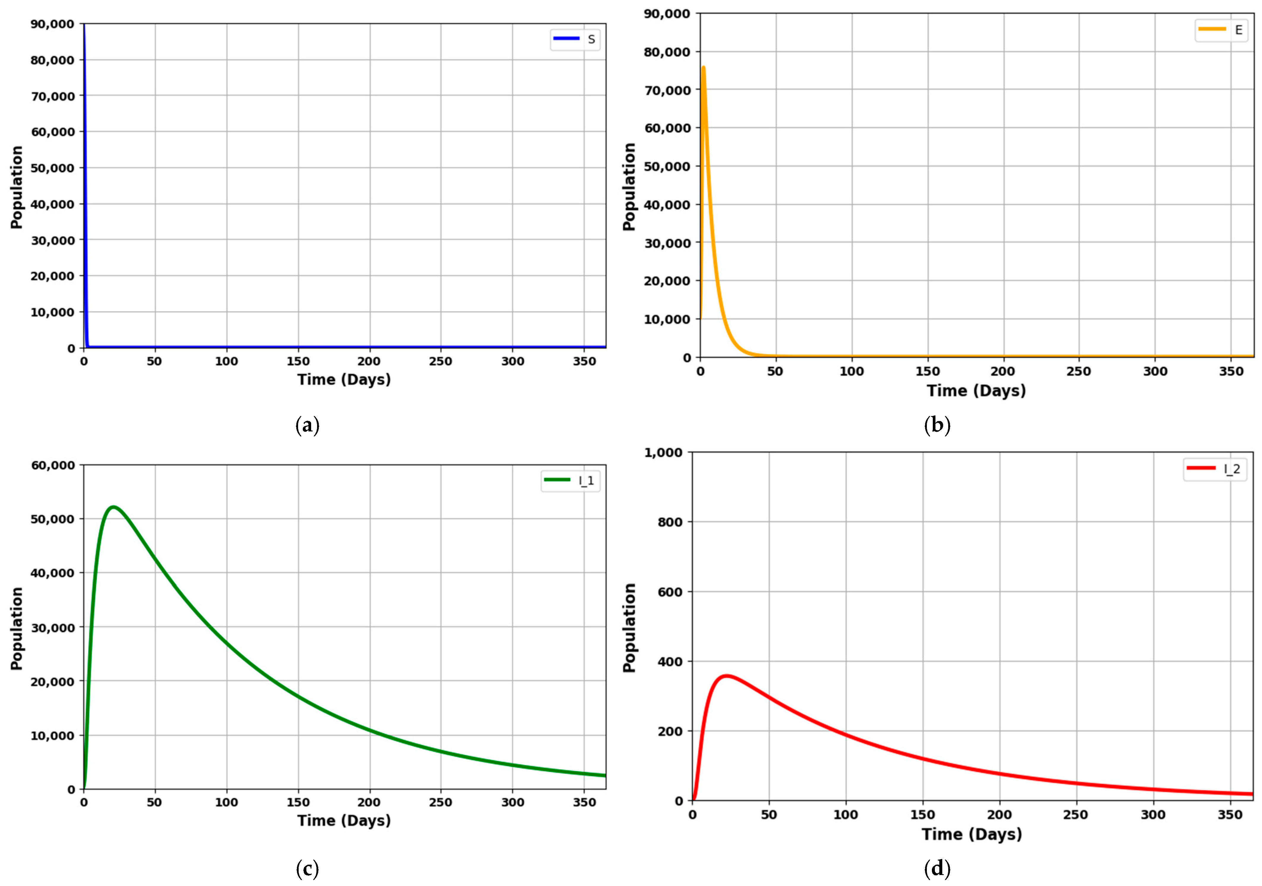
Figure 8a–h depicts the dynamics of an infectious disease over 365 days, given that R₀ = 1.7045 (which is greater than 1).

• Figure 8a shows a rapid decrease in the vulnerable (susceptible) population.
• Figure 8b depicts a steady rise in the exposed population, which then gradually declines.
• Figure 8c,d illustrate the rates of asymptomatic individuals at an early stage and symptomatic individuals at a later stage, showing an initial increase followed by a significant drop.
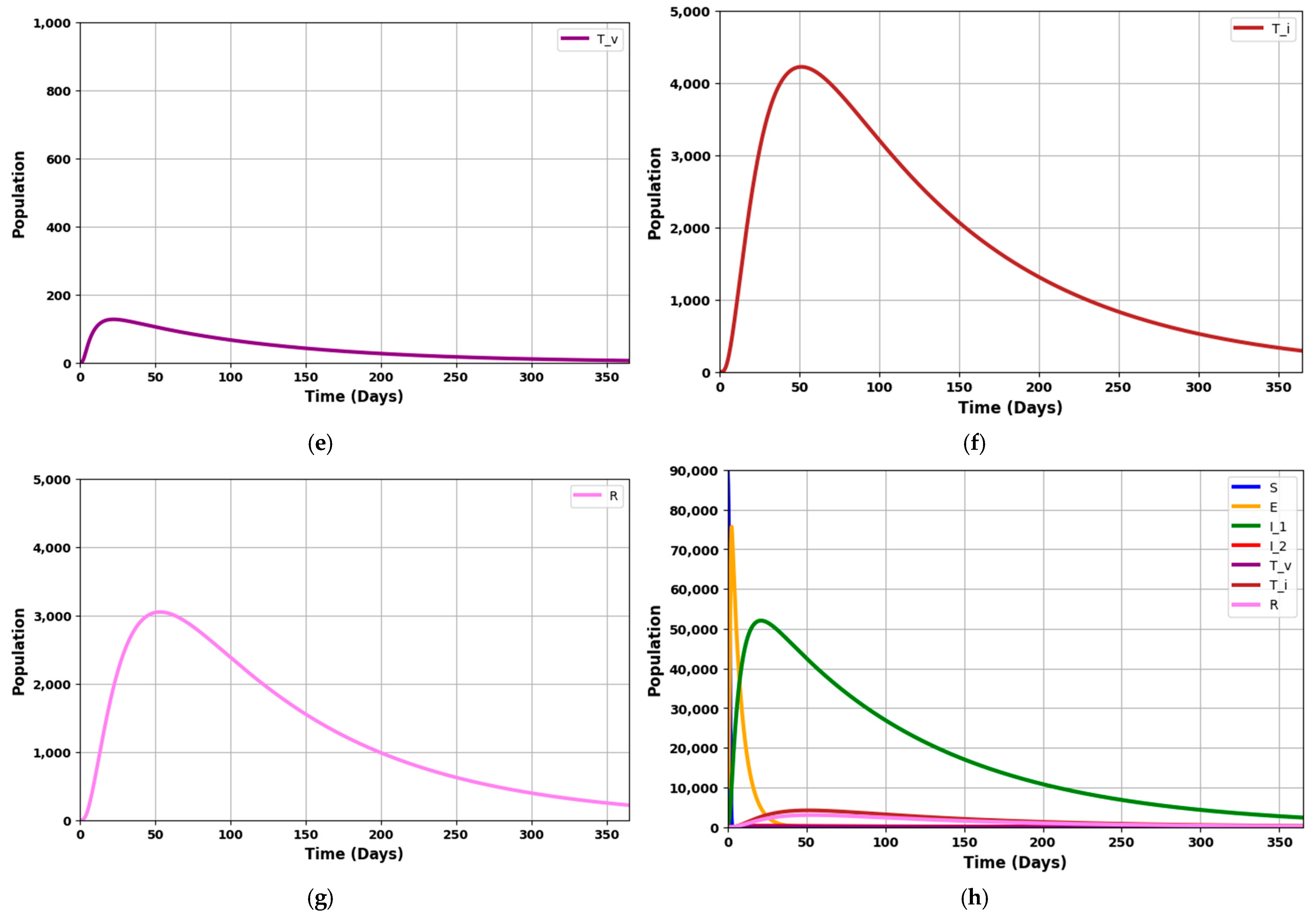
• Figure 8e,f reflects the number of patients requiring mechanical ventilation and ICU treatment, which increases over time and decreases as the counts of asymptomatic and symptomatic patients fall.
• Figure 8g displays the recovery rate, which rises until the fifteenth week before gradually tapering off.

The graphs model the progression of the disease through different stages. The susceptible population (S) declines as individuals become exposed (E) to the infection. The exposed group initially grows but then decreases as these individuals progress to the infected stages (I₁ and I₂). The I₁ group initially rises but then stabilizes or decreases as individuals recover or advance to the more severe I₂ stage. The I₂ group grows more slowly and represents the more severe cases.

The treated or isolated population (T_v) gradually increases, reflecting the impact of treatment and isolation measures in controlling the disease spread. Lastly, the recovered population (R) steadily grows as individuals recover, which helps to reduce the overall disease burden on the population.

These figures illustrate the disease’s spread, progression, and eventual control through recovery and interventions, showing how the various stages of infection evolve.

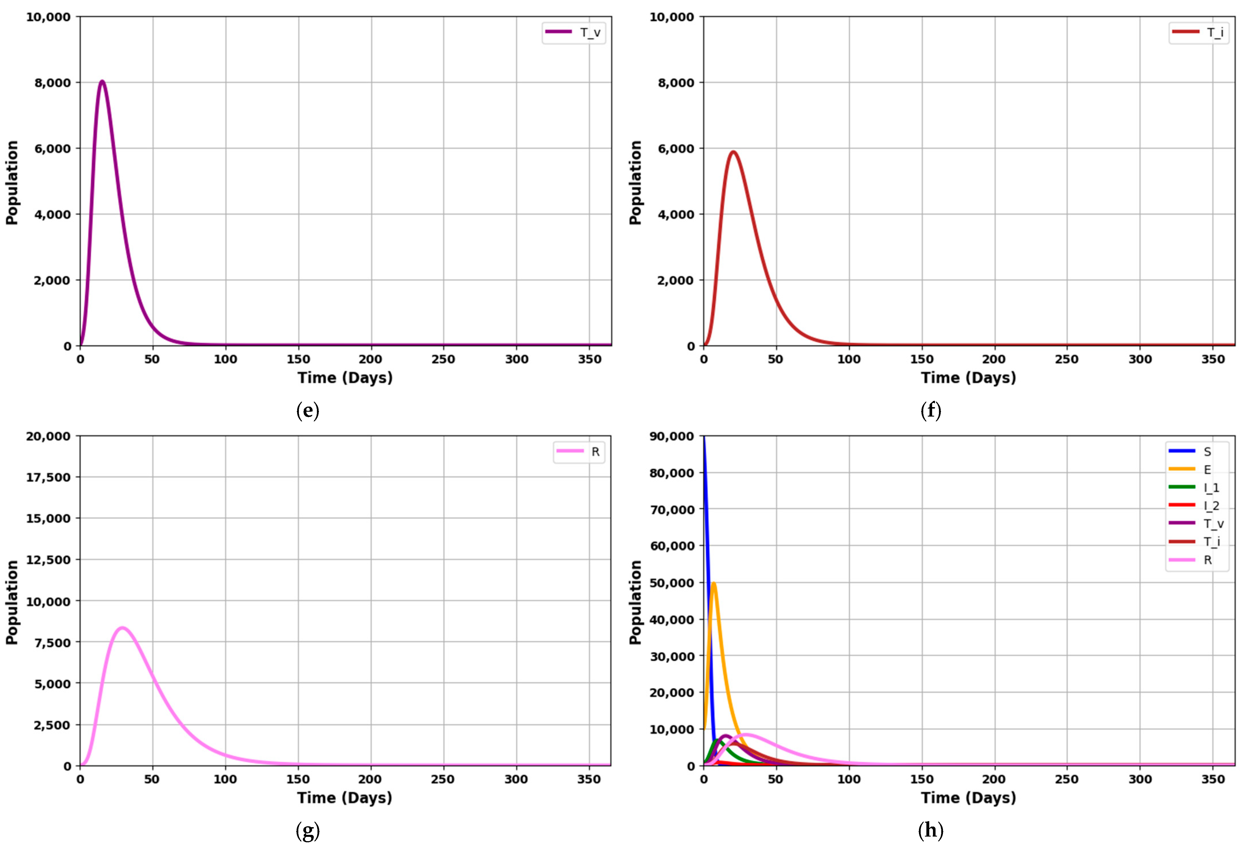
The simulation will employ the parameters listed in Table 3. These parameter values, sourced from various literature, have been chosen to illustrate specific theoretical results obtained in this study, particularly in scenarios where 0 < R₀ < 1.

Figure 9a: This compartment captures the population of individuals at risk of contracting the disease but has not yet been exposed. The dynamics of this group are governed by the rate of new infections, which is influenced by the transmission parameter ($\beta$) and the presence of infected individuals. A decreasing trend in the susceptible population reflects successful disease transmission and a reduction in the pool of potentially exposed individuals. Figure 9b: This compartment represents individuals exposed to the pathogen but is not yet infectious. The increase in this group corresponds to new exposures from susceptible individuals becoming infected. The rate of change is influenced by the transmission dynamics and the progression rate from exposed to infectious states ($\lambda$). Over time, a decrease in the exposed population indicates a transition to the infected stages or a reduction in new exposures. Figure 9c: This group includes individuals in the first infection stage. The rate of change in this compartment is determined by the transition from the exposed state ($\lambda$) and progression to the next infection stage ($\gamma$,${\epsilon }_1$, ${\tau }_1$). Fluctuations in the I₁ population reflect the interplay between new infections and the progression to I₂. High values suggest a large number of new infections or slow progression. Figure 9d: Represents individuals in the second stage of infection. These compartment dynamics are driven by the progression from I₁ and the rates of treatment and natural disease progression ($\gamma$, $\psi ,{\epsilon }_1$,${ \tau }_2$). Changes in this population indicate the severity and stage of the disease. A rising I₂ population may suggest a delay in progression or inadequate treatment, while a decrease indicates recovery or effective intervention. Figure 9e: This compartment tracks individuals receiving specific treatments such as mechanical ventilation. The size of this group is influenced by the number of severe cases from I₂ and the effectiveness of interventions ($\sigma ,{\phi }_v$). The dynamics here reflect the capacity and effectiveness of critical care interventions. A decreasing trend may indicate recovery or transfer to other treatment stages. Figure 9f: Represents individuals undergoing intensive care unit (ICU) treatment. The dynamics of this compartment are influenced by severe disease cases and the rate of transitioning from Treated under ventilation ($\sigma ,\alpha$). Fluctuations in this group provide insights into the burden on intensive care resources and the overall severity of the disease. A decrease might signal recovery or movement to less intensive care. Figure 9g: This compartment includes individuals who have recovered from the infection, through natural immunity or successful treatment. The rate of change in the recovered population is influenced by the recovery rates from various treatment stages and natural recovery processes ($\alpha ,{\phi }_v, {\phi }_i, {\epsilon }_1$). An increasing R line signifies effective treatment and recovery processes, reflecting the overall success of disease management and intervention strategies.

The graph provides a comprehensive view of the disease progression, treatment impact, and recovery dynamics. It highlights how each compartment interacts with the others and how different parameters affect the overall epidemic trajectory. In summary, with R₀ = 0.9703, the figures collectively demonstrate a scenario where the disease is trending towards decline. They show how the various population groups evolve, highlighting the reduction in infection rates, the effectiveness of treatment strategies, and the progressive increase in the recovered population.

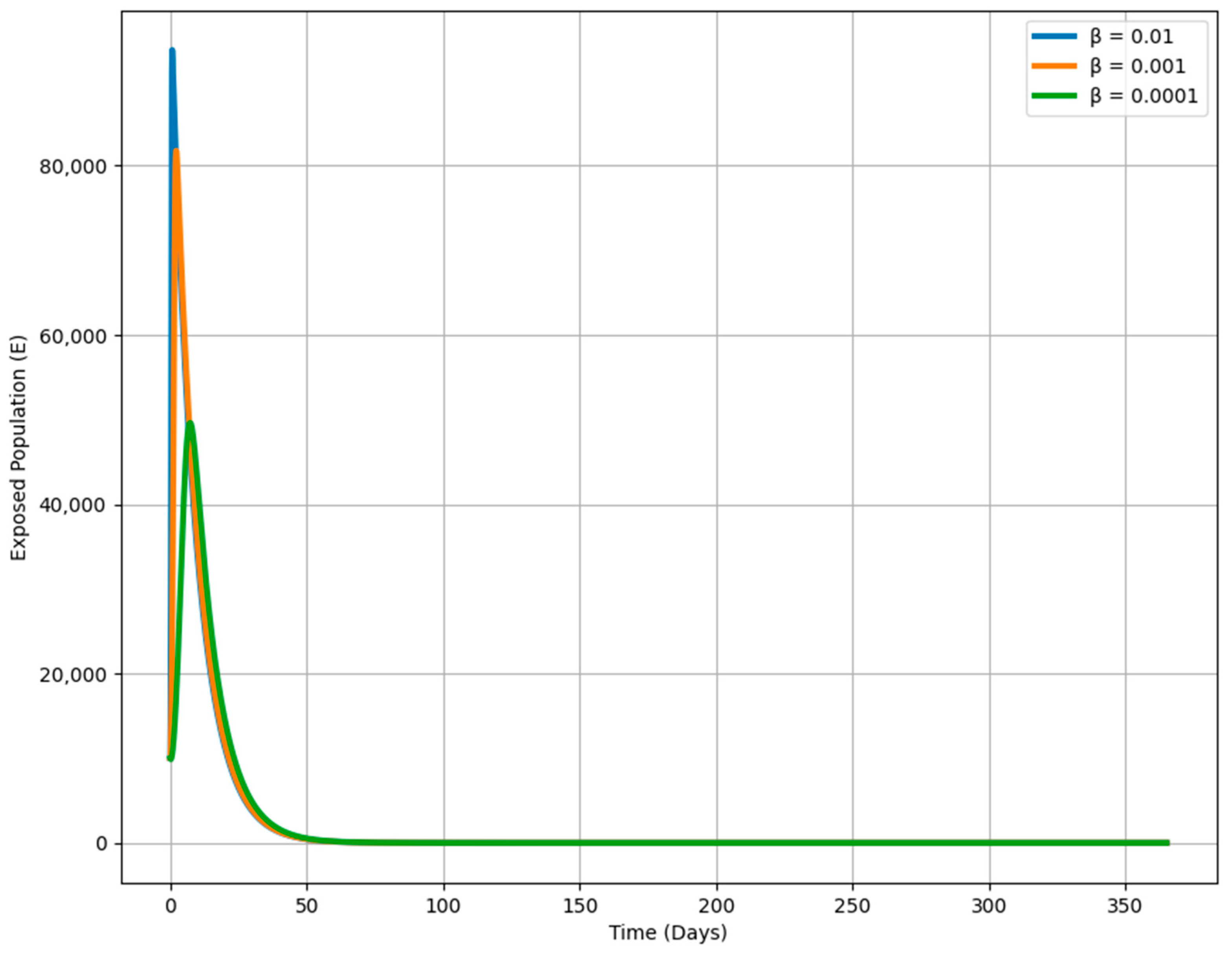
Figure 10 shows how varying the transmission rate (β) affects the dynamics of the exposed population over time in an epidemiological model. Each curve corresponds to a different β value, which determines the speed at which susceptible individuals become exposed when they encounter infectious individuals. A higher β (e.g., 0.01) leads to a rapid and large increase in the exposed population, reflecting a fast-spreading disease. Conversely, a lower β (e.g., 0.0001) results in a much slower rise, indicating a slower spread and a smaller exposed population. This visualization highlights the critical impact of β on the outbreak’s trajectory, demonstrating that reducing the transmission rate through public health measures like social distancing or vaccination can flatten the curve, slowing the spread and reducing the number of exposed individuals over time.

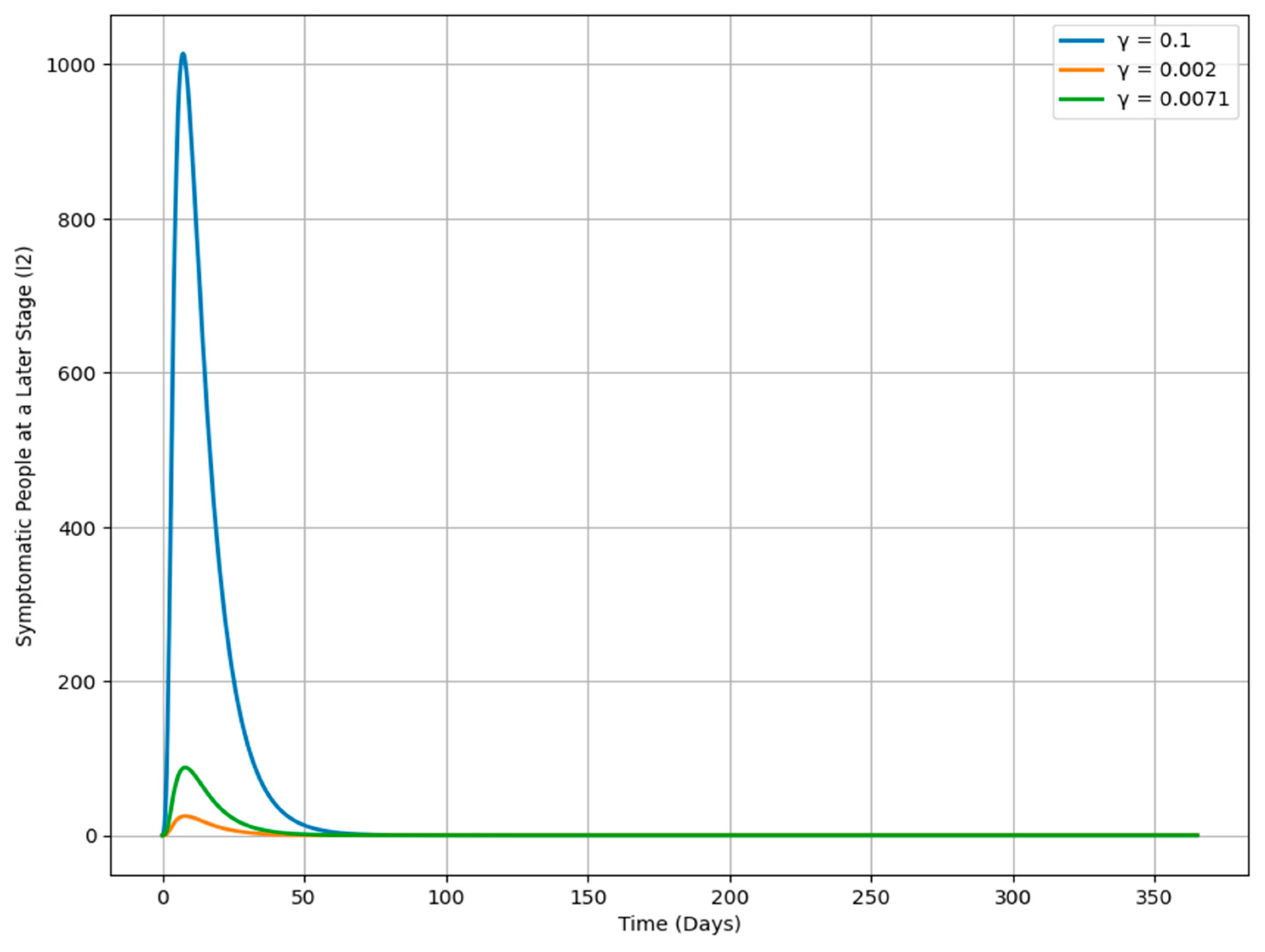
Figure 11 shows how changes in the progression rate γ affect the dynamics of the I₂ population over time, with each curve representing a different γ value. When γ is higher (e.g., 0.1), the I₂ population increases more rapidly, indicating a quicker transition from the I₁ class to the more advanced I₂ stage, leading to a swift accumulation of severe cases. In contrast, a lower γ (e.g., 0.002) results in a slower rise in the I₂ population, meaning individuals remain in the I₁ class longer before progressing, corresponding to a less aggressive disease progression. A moderate γ (e.g., 0.0071) leads to a more balanced increase in the I₂ population, sitting between the high and low γ scenarios. This analysis highlights the significant role of γ in determining the trajectory of an infection, offering important insights for public health strategies aimed at managing disease spread and severity by adjusting the rate of progression between different stages of infection.

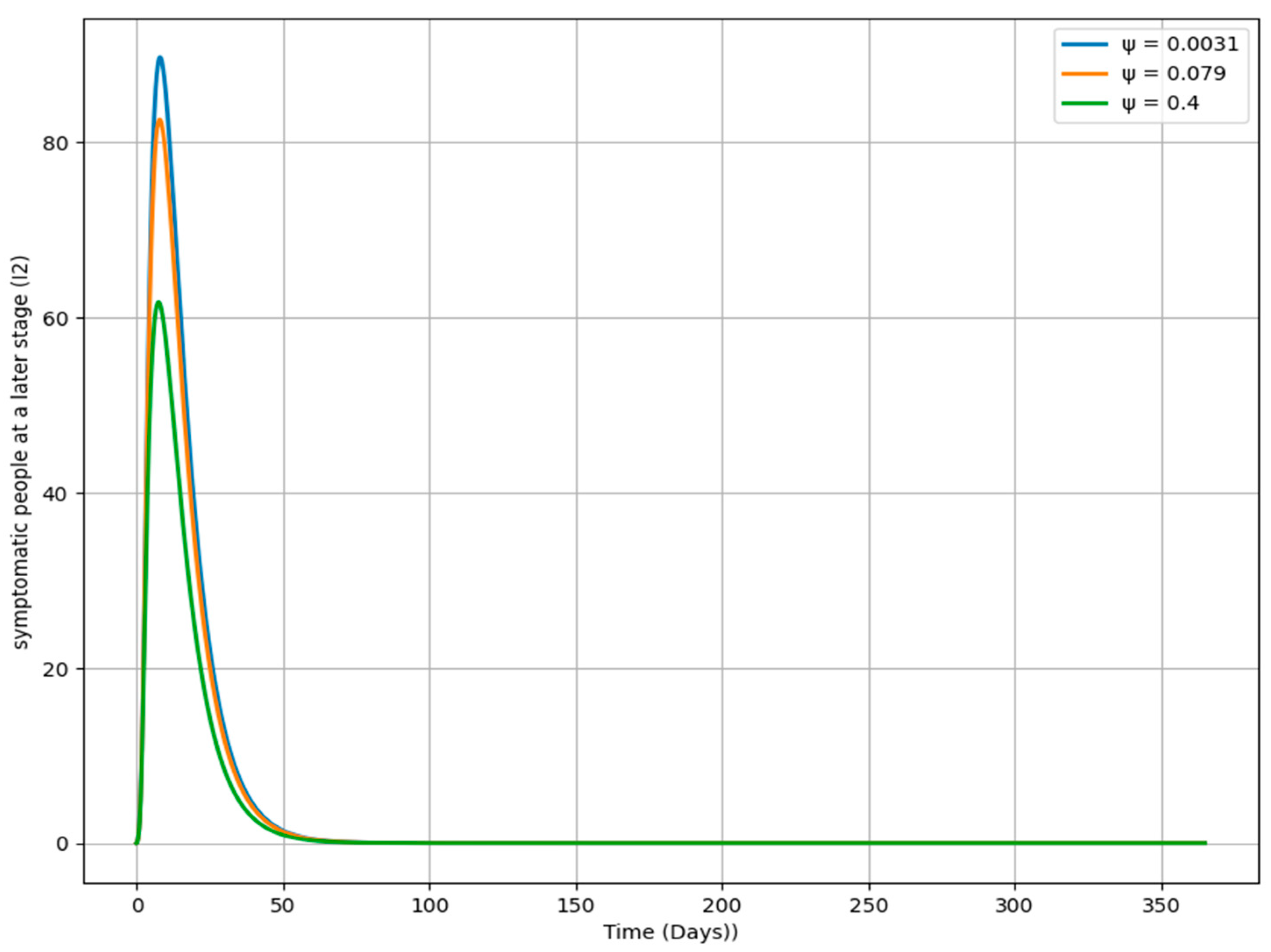
Figure 12 illustrates the impact of varying the rate ψ on the dynamics of the I₂ population over time. Each curve represents a different ψ value, determining how quickly individuals transition from the I₂ class to the T_v class. A higher ψ value (e.g., 0.4) leads to a faster decline in the I₂ population, indicating that individuals quickly move out of the I₂ stage. Conversely, a lower ψ value (e.g., 0.0031) results in a slower decrease, suggesting that individuals remain in the I₂ stage longer, potentially leading to a more prolonged infection period. The moderate ψ value (e.g., 0.079) produces a decline in the I₂ population that is intermediate between the high and low ψ scenarios. This analysis highlights the critical role of ψ in influencing the duration and severity of the infection in the I₂ class, offering insights into how different rates of progression can shape the overall trajectory of the disease.

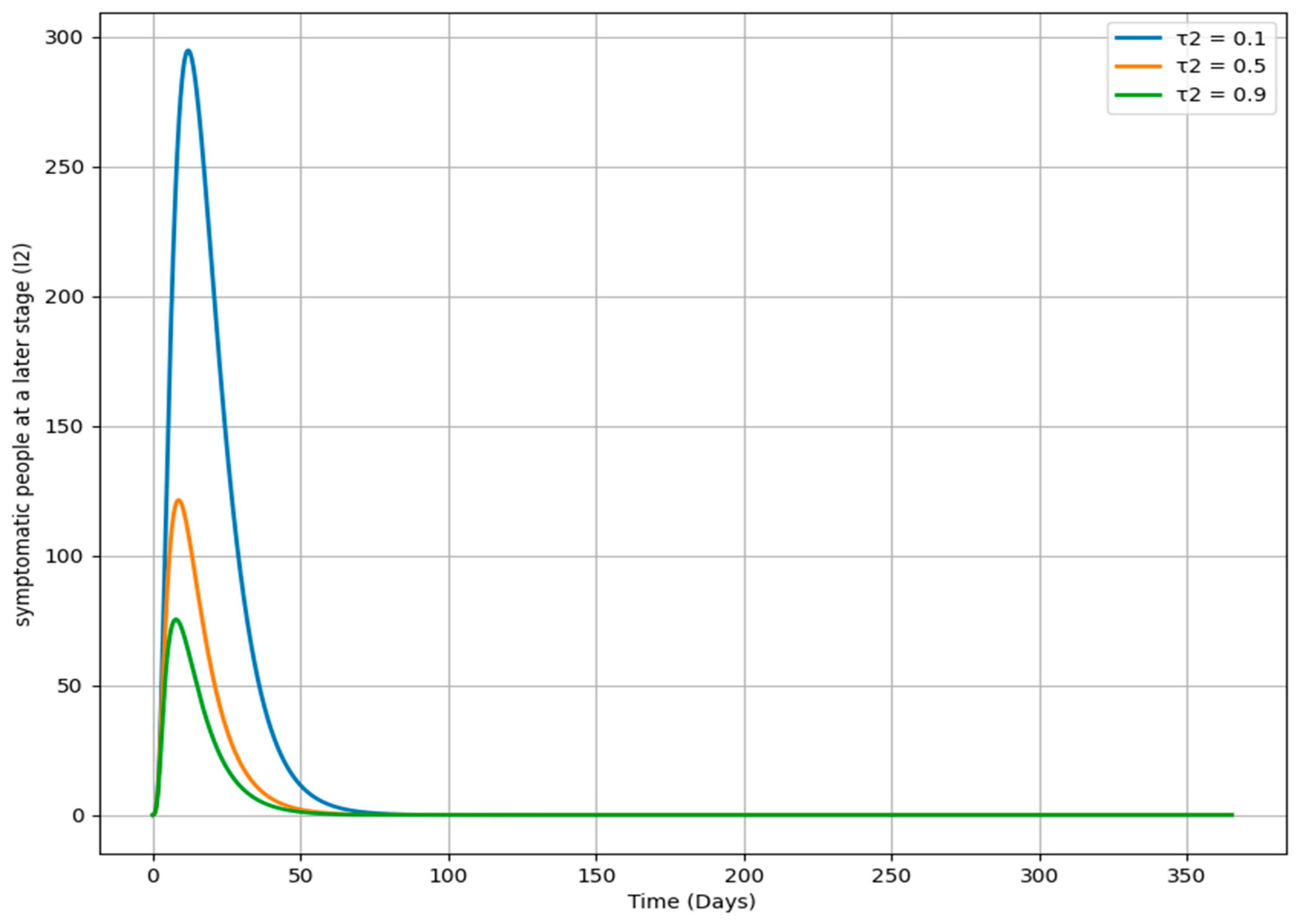
Figure 13 demonstrates how changes in the parameter τ₂, which governs the rate at which individuals move from the I₂ class to the T_i class, impact the dynamics of the I₂ population over time. Each curve represents a different τ₂ value. A higher τ₂ (e.g., 0.9) leads to a faster decrease in the I₂ population, suggesting that individuals are swiftly transitioning out of the I₂ class, likely due to prompt treatment or isolation. In contrast, a lower τ₂ (e.g., 0.1) results in a slower decline, indicating that individuals stay longer in the I₂ class, potentially due to delays in intervention. The curve for a moderate τ₂ (e.g., 0.5) shows a balanced transition rate. This analysis highlights the importance of τ₂ in managing the length and intensity of infection within a population, offering valuable insights for public health strategies focused on enhancing the timing and efficacy of interventions to mitigate the impact of the disease.

6. Conclusions

This study investigated the transmission dynamics of the herpes simplex virus (HSV) through a mathematical model, specifically the compartmental model SEITR (susceptible-exposed-infectious-treated-recovered), to gain insights into how HSV spreads across different stages of infection. The analysis of the model revealed key findings regarding the system’s stability, the factors influencing the spread of the disease, and potential control strategies.

The results indicate that the system behaves differently under disease-free and disease-active conditions, as represented by the primary reproduction number (R₀). When R₀ < 1, the system is locally asymptotically stable, and the infection will eventually die out, suggesting that reducing the number of new infections is critical to disease control. On the other hand, when R₀ ≥ 1, global asymptotic stability is achieved, meaning the infection will persist unless further intervention occurs. These findings emphasize the importance of reducing R₀ through public health measures and treatment interventions to control HSV transmission.

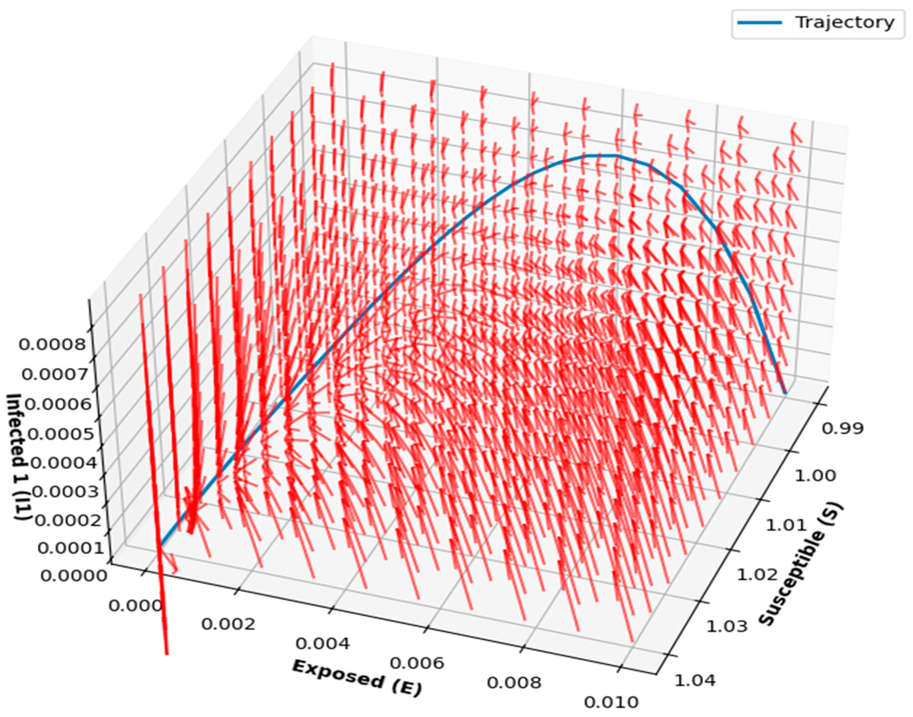
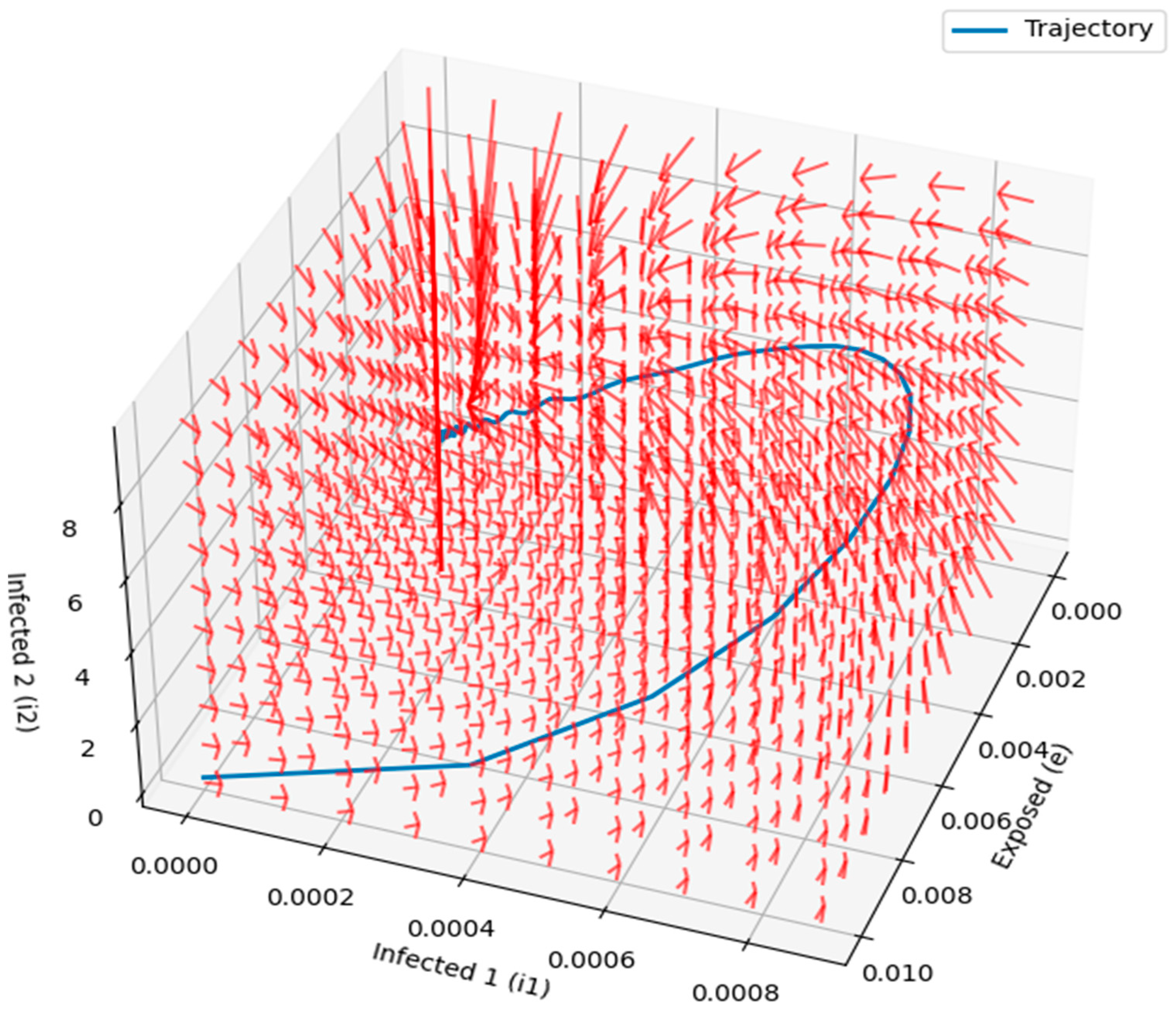
Figure 14 and Figure 15 provided detailed visualizations of the disease dynamics in the compartmental model, illustrating the interactions between susceptible, exposed, and infected individuals. The 3D phase portraits and vector fields helped demonstrate the progression of the disease and the rate at which individuals transition between states, highlighting the factors that influence disease spread. The vector field, with longer arrows indicating faster transitions, provided valuable insights into the speed and direction of disease dynamics at different stages. These visualizations offer an intuitive understanding of the disease’s progression, stability, and critical intervention points, making them useful for designing effective control strategies.

A comprehensive sensitivity analysis revealed that the interactions between susceptible individuals and those in asymptomatic, symptomatic, or infected stages play a crucial role in driving the transmission dynamics of HSV. The analysis also identified which parameters, such as transmission and recovery rates, have the most significant impact on the spread of the disease. By incorporating real-world data fitting, we were able to illustrate how variations in these parameters could influence the course of an outbreak.

However, the study has certain limitations. First, the model is based on available literature and generalized assumptions due to the lack of specific real-world datasets on herpes simplex encephalitis. While this approach provided valuable insights, the accuracy of the model’s predictions could be enhanced with more precise and region-specific data. Additionally, while we incorporated several stages of infection, the model did not account for all possible variables, such as co-infections or environmental factors, which could further influence disease transmission.

Future research should focus on refining the model by incorporating more detailed data on HSV transmission, particularly from real-world outbreaks, to increase the model’s precision. Including additional factors like co-infections, environmental influences, and public health interventions could improve the robustness of the model. Further studies should also explore different intervention strategies and their potential impact on reducing R₀ and ultimately controlling the spread of HSV.

In conclusion, this study provides a valuable framework for understanding the dynamics of HSV transmission and highlights the importance of reducing R₀ in managing outbreaks. The model’s flexibility and the insights from the sensitivity analysis can inform future research and public health strategies aimed at controlling the spread of herpes simplex encephalitis and similar infectious diseases.