Takagi–Sugeno–Kang Fuzzy Neural Network for Nonlinear Chaotic Systems and Its Utilization in Secure Medical Image Encryption

Abstract

This study introduces a novel control framework based on the Takagi–Sugeno–Kang wavelet fuzzy neural network, integrating brain imitated network and cerebellar network. The proposed controller demonstrates high robustness, making it an excellent candidate for handling intricate nonlinear dynamics, effectively mapping input–output relationships and efficiently learning from data. To enhance its performance, the controller’s parameters are fine-tuned using Lyapunov stability theory. Compared to existing approaches, the proposed model exhibits superior learning capabilities and achieves outstanding performance metrics. Furthermore, the study applies this synchronization technique to the secure transmission of medical images. By encrypting a medical image into a chaotic trajectory before transmission, the system ensures data security. On the receiving end, the original image is successfully reconstructed using chaotic trajectory synchronization. Experimental results confirm the effectiveness and reliability of the proposed neural network model, as well as the encryption and decryption process. Specifically, the average_RMSE of the Takagi–Sugeno–Kang fuzzy wavelet brain cerebral controller (TFWBCC) method is 2.004 times smaller than the cerebellar model articulation controller (CMAC) method, 1.923 times smaller than the RCMAC method, 1.8829 times smaller than the TSKCMAC method, and 1.8153 times smaller than the brain emotional learning controller (BELC) method.

1. Introduction

With the rapid spread of the Internet, e-health is becoming more widespread and accessible. This approach, also known as e-healthcare, uses digital and telecommunications technologies—such as computers, mobile devices and online networks—to improve medical services. E-healthcare is often integrated with traditional healthcare to provide patients and healthcare consumers with direct access to medical information [1,2,3]. However, when confidential images are subjected to cryptanalysis, sensitive data may be exposed, which could jeopardize individual privacy. Therefore, ensuring the security of medical image data has become an important priority [4,5,6].

To safeguard sensitive medical data, patient images must undergo anonymization through encryption. Accessing the original image requires the use of a precise decryption key [7,8,9]. Medical images possess unique characteristics, including strong pixel correlation, large data size, and significant redundancy [10,11,12]. Encryption techniques such as tent maps and bit-plane manipulation can be employed to secure these images. Consequently, ensuring robust security measures for both the transmission and storage of digital medical images is essential.

In recent years, researchers have extensively explored the synchronization of chaotic trajectories, a topic that has garnered significant scientific attention. Chaotic synchronization refers to the phenomenon where initially uncoordinated chaotic systems evolve into a state of organized behavior over time, offering valuable insights into the dynamics of complex systems. Several studies have examined the application of the 3D Lorenz chaotic system for secure data transmission [13,14] and investigated methods to synchronize chaotic systems for enhancing secure communication [15,16].

The interest in chaotic synchronization stems from the intricate and partially unexplored characteristics of chaotic behavior. This field holds critical relevance across various domains, including secure communications, control engineering, robotics, neuroscience, information processing, and biomedical applications. Despite its promising potential, chaotic systems present significant challenges due to their inherent unpredictability and highly nonlinear properties, making their control and synchronization a complex endeavor.

In modern times, model-free approaches have become increasingly popular for describing systems with unpredictable and random properties in both structure and parameters. A growing challenge in control theory is the need for precise management of complex systems. While traditional control techniques are effective in well-defined, stable, and linear environments, they struggle to cope with the complexity and uncertainty inherent in nonlinear chaotic systems [17,18]. Although adaptive controllers offer partial solutions, they remain difficult to implement in high-dimensional datasets or unstructured environments [19,20].

To address these challenges, extensive research has focused on fuzzy mathematical models, which emulate human-like reasoning [21,22,23,24]. Fuzzy systems are broadly categorized into two types: the Takagi–Sugeno–Kang (TSK) fuzzy systems and the Mamdani–Larsen fuzzy systems. The Mamdani–Larsen approach is known for its linguistic clarity, robustness, and rule-based structure, making it suitable for interpretability and smooth decision-making. On the other hand, TSK fuzzy systems excel in function approximation, offering simpler rule bases, superior nonlinear modeling, fast learning, flexibility, and effective parameterization for optimization techniques. These properties make TSK fuzzy models particularly suitable for handling intricate nonlinear relationships between input and output variables and for efficient training using data. A deep TSK fuzzy classifier with a hierarchical architecture and interpretable linguistic rules has been developed and tested through computational experiments and real-world applications [25]. Additionally, TSK fuzzy systems have been widely used in domains such as finance, medicine, and intelligent control systems [26,27].

Despite their advantages, fuzzy control in chaotic systems remains challenging due to issues such as inherent imprecision, the complexity of designing rule bases, difficulty in tuning membership functions, high implementation costs, and limited theoretical guarantees. Furthermore, fuzzy controllers may struggle to adapt to external disturbances and parameter uncertainties, leading to synchronization errors and increased system complexity.

In recent years, neural networks (NNs) have gained significant attention across multiple scientific and engineering disciplines for their capacity to handle complex nonlinear functions [28,29]. Neural networks are particularly powerful in modeling complex systems, function approximation, and integrating diverse data sources. Several biologically inspired neural architectures have been investigated, including the brain emotional learning controller (BELC) [30], the cerebellar model articulation controller (CMAC) [31,32], RNN [33,34], radial basis function neural network (RBFNN) preprocessors combined with CMAC [35,36], and fuzzy neural networks (FNN) [37,38].

Neural networks possess several advantages, including the ability to process imprecise information, integrate human expertise, perform parallel computations, and exhibit high fault tolerance, making them well-suited for controlling complex systems. However, controlling chaotic systems remains highly challenging due to their sensitivity to initial conditions. The design and training of neural network controllers require careful selection of network architecture, data, and learning algorithms. Additionally, neural networks demand vast amounts of training data, involve computationally intensive architectures, and may face challenges in generalizability—controllers optimized for one system may not necessarily perform well for another.

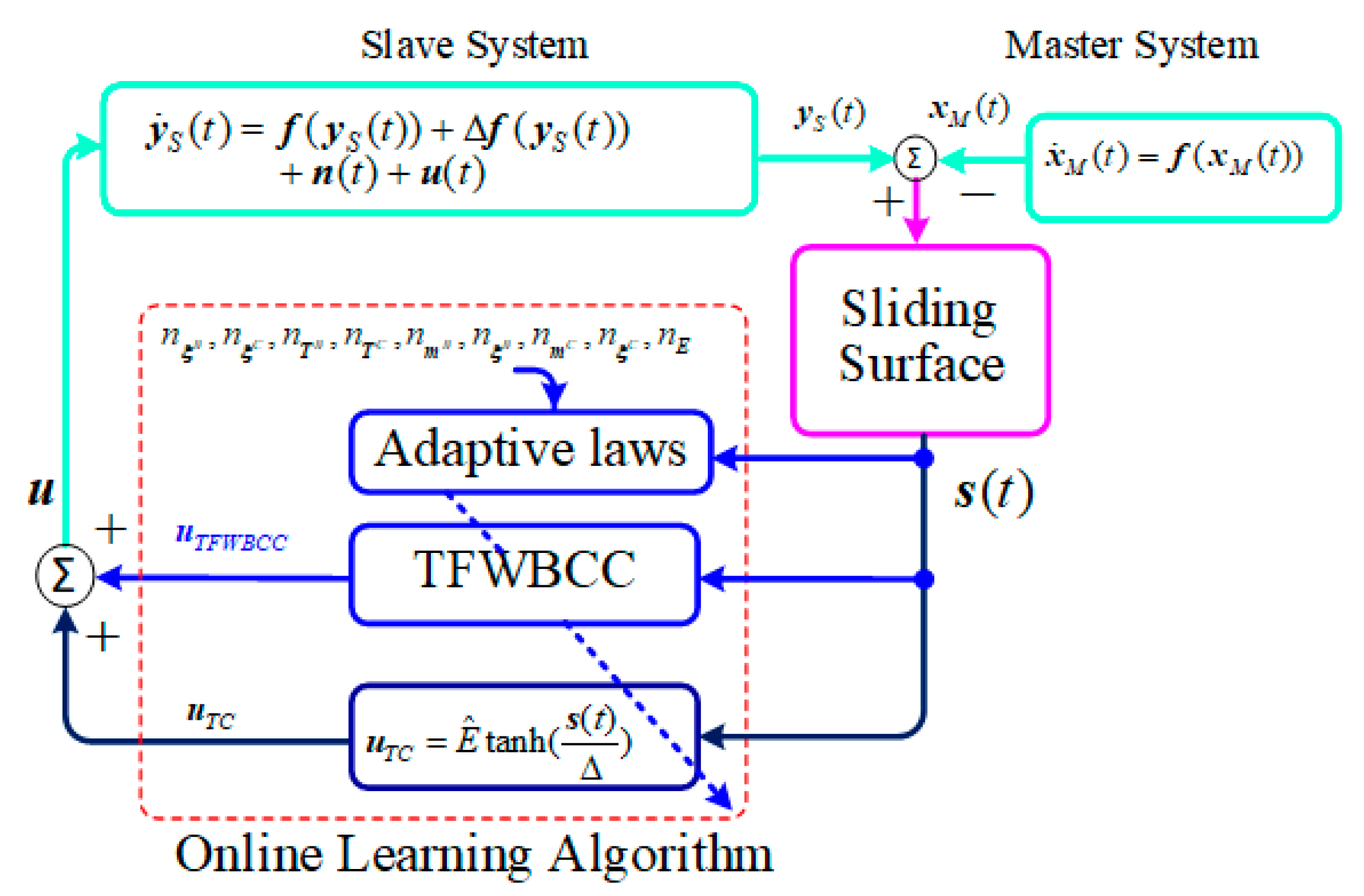
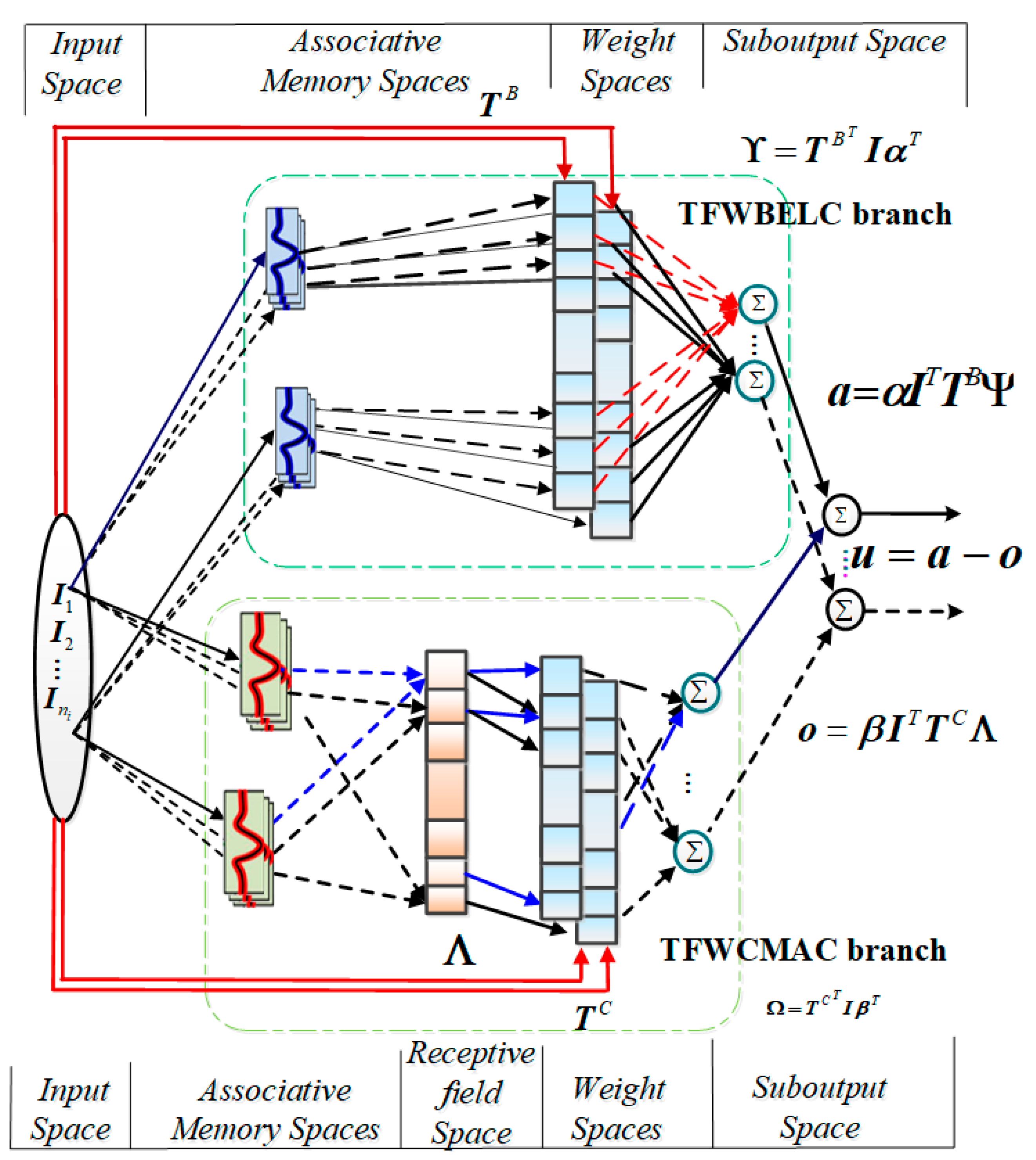
The proposed method integrates the strengths of wavelet features with Takagi–Sugeno–Kang fuzzy system (TSKFS) to create a TSK fuzzy wavelet brain cerebellar controller (TFWBCC). The effectiveness of the method is demonstrated by simulating 4D hyperchaotic synchronization. The main contributions of this work are as follows:

(1)

A novel wavelet function is incorporated into the BELC and CMAC channels and improves their ability to account for uncertainty in the membership function. This approach utilizes TSKFS for dual-channel CMAC and BELC and enables more flexible parameter updates, improved mapping capabilities, and precise approximation performance.

(2)

A TFWBCC is proposed to achieve synchronization in hyperchaotic systems.

(3)

The stability of the proposed system is rigorously verified using Lyapunov stability theory.

This paper is structured as follows: The first section provides an overview of the problem being addressed. In the second section, the proposed TFWBCC approach for achieving chaotic system synchronization is detailed, along with an explanation of how the Lyapunov method is utilized to update the controller parameters, Section 3 shows the proposed TFWBCC for 4D hyper master and slave chaotic synchronization and its application for medical secure image transmission. Section 4 presents the numerical simulation results for the 4D hyperchaotic in MATLAB software. Section 5 presents the medical image encryption using 4D hyper chaotic synchronization. Finally, Section 6 presents the conclusion of the paper. To make it easier to understand the abbreviations, you can see the list of abbreviations used in this article in

Table 1. List of abbreviations used in the article.

Symbol	Meaning
TFWBCC	Takagi–Sugeno–Kang Fuzzy Wavelet Brain Cereberal Controller
CMAC	Cerebellar Model Articulation Controller
BELC	Brain Emotional Learning Controller
RNN	Recurrent Neural Network
RBFNN	Radial Basis Function Neural Network
FNN	Fuzzy Neural Networks
NN	Neural Network
TSKFS	Takagi–Sugeno–Kang Fuzzy System
TWBC	Takagi–Sugeno–Kang Wavelet Brain Emotional Learning Controller
TFWCC	Takagi–Sugeno–Kang Wavelet Cerebellar Controller

.

The primary differences between the proposed control strategy and conventional methods are presented in

Table 2. Key distinctions of the proposed control approach compared to existing methods.

Method	Main Advance of Methods	Robust Compensator and Convergence Analysis
Our method	Consisting TSK fuzzy system to update weights of two both channels CMAC and BELC, and using wavelet function for approximate the uncertainty of inputs more effectively.	Using tanhypeboloic function as an compensate the intelligent controler with the ideal controller. Then, using Lapunov theory to propose the convergence of the proposed control system.
TSK FBELC [13]	Only use Gausian function for normailize the uncertainty of the input.	Only use sign function to compensate the intelligent controller with the ideal controller.
Type-2 FNN [31]	Only using fuzzy inference system not use TSK fuzzy system	Only use sign function to compensate the intelligent controller with the ideal controller.
Improved CMAC [35]	Using the convergence speed of CMAC to improve the trajectory tracking performance.	Using tanhypeboloic function as an compensate the intelligent controler with the ideal controller, and using Lyapunov function to propose the convergence of the control system
Function-link fuzzy CMAC [39]	Using the convergence speed of CMAC to improve the trajectory tracking performance.	Using tanhypeboloic function as an compensate the intelligent controler with the ideal controller, and using Lyapunov function to propose the convergence of the control system

.

2. Problem Formulation

Generic four-dimensional master systems, which can be represented as follows:

$$\{\begin{array}{l}{\dot{x}}_{M1}(t)=f_1(x_{Mi})\\ {\dot{x}}_{M2}(t)=f_2(x_{Mi})\\ {\dot{x}}_{M3}(t)=f_3(x_{Mi})\\ {\dot{x}}_{M4}(t)=f_4(x_{Mi})\end{array}$$

(1)

where $x_{Mi}$ and $f_i (i=1,2,3,4)$ are, respectively, the states of the master system and nonlinear functions.

The typical structure of the slave system is outlined below:

$$\{\begin{array}{l}{\dot{y}}_{S1}(t)=f_1(y_{Si})+\mathsf{\Delta }f(y_{S1})+n_1+u_1\\ {\dot{y}}_{S2}(t)=f_2(y_{Si})+\mathsf{\Delta }f(y_{S2})+n_2+u_2\\ {\dot{y}}_{S3}(t)=f_3(y_{Si})+\mathsf{\Delta }f(y_{S3})+n_3+u_3\\ {\dot{y}}_{S4}(t)=f_4(y_{Si})+\mathsf{\Delta }f(y_{S4})+n_4+u_4\end{array}$$

(2)

where $y_{Si}$, $n_i$, $u_i$, and $\mathsf{\Delta }f(y_{Si}) (i=1,2,3,4)$ are, respectively, system states, unknown external disturbances, control inputs, and uncertainties of the system. If a proper control input $u_i$, $(i=1,2,3,4)$ is structured to ensure that the slave’s states align with those of the master. It indicates that both systems operate in perfect harmony, thus, ${\lim }_{t\to \infty }\left|y_{Si}(t)-x_{Mi}(t)\right|\to 0$. Take into account a particular instance of a four-dimensional hyperchaotic master system, as described in reference [38]:

$$\{\begin{array}{l}{\dot{x}}_{M1}=-a(x_{M2}-x_{M1})+x_{M4}\\ {\dot{x}}_{M2}=b{x}_{M1}-x_{M1}{x}_{M3}+x_{M4}\\ {\dot{x}}_{M3}=x_{M1}{x}_{M2}-x_{M3}-x_{M4}\\ {\dot{x}}_{M4}=-c\left(x_{M1}+x_{M2}\right)\end{array}$$

(3)

in which the exact values $a, b, \mathrm{and} c$ can be determined, allowing the slave system to be represented as follows:

$$\{\begin{array}{l}{\dot{y}}_{S1}=-a\left(y_{S2}-y_{S1}\right)-y_{S4}+\mathsf{\Delta }Y(y_{S1})+n_{d1}+u_1\\ {\dot{y}}_{S2}=b{y}_{S1}-y_{S1}{y}_{S3}+y_{S4}+\mathsf{\Delta }Y(y_{S2})+n_{d2}+u_2\\ {\dot{y}}_{S3}=y_{S1}{y}_{S2}-y_{S3}-y_{S4}+\mathsf{\Delta }Y(y_{S3})+n_{d3}+u_3\\ {\dot{y}}_{S4}=-c\left(y_{S1}+y_{S2}\right)+\mathsf{\Delta }Y(y_{S4})+n_{d4}+u_4\end{array}$$

(4)

where $\mathit{u}={[u_1,u_2,u_3,u_4]}^T$ is the control input vector, ${\mathit{n}}_d={[n_{d1},n_{d2},n_{d3},n_{d4}]}^T$ is the unknown external disturbance, $\mathsf{\Delta }\mathit{Y}(y_S)={\left[\mathsf{\Delta }Y(y_{S1}),\mathsf{\Delta }Y(y_{S2}),\mathsf{\Delta }Y(y_{S3}),\mathsf{\Delta }Y(y_{S4})\right]}^T$ is the uncertainty of the system, and $y_{Si} (i=1,2,3,4)$ is the slave state. The tracking error can be calculated as follows:

$$\{\begin{array}{l}{e}_1=y_{1S}-x_{1M}\\ e_2=y_{2S}-x_{2M}\\ e_3=y_{3S}-x_{3M}\\ e_4=y_{4S}-x_{4M}\end{array}$$

(5)

The measurement of the tracking discrepancy is determined as follows:

$$\{\begin{array}{l}{\dot{e}}_1={\dot{y}}_{S1}-{\dot{x}}_{M1}=-a(e_2-e_1)-e_4+\mathsf{\Delta }Y(y_{S1})+n_{d1}+u_1\\ {\dot{e}}_2={\dot{y}}_{S2}-{\dot{x}}_{M2}=b{e}_1-y_{S1}{y}_{S3}+x_{M1}{x}_{M3}+\mathsf{\Delta }Y(y_{S2})+n_{d2}+u_2\\ {\dot{e}}_3={\dot{y}}_{S3}-{\dot{x}}_{M3}=y_{S1}{y}_{S2}-x_{M1}{x}_{M2}-e_4+\mathsf{\Delta }Y(y_{S3})+n_{d3}+u_3\\ {\dot{e}}_4={\dot{y}}_{S4}-{\dot{x}}_{M4}=-c(e_1+e_2)+\mathsf{\Delta }Y(y_{S4})+n_{d4}+u_4\end{array}$$

(6)

Rewriting Equation (6) to the vector form as follows:

$$\dot{\mathit{e}}=\mathsf{\Pi }\mathit{e}+\mathsf{\Omega }+\mathsf{\Delta }Y({\mathit{y}}_S)+{\mathit{n}}_d+\mathit{u}$$

(7)

where $\mathsf{\Pi }=\left[\begin{array}{cccc}a& -a& 0& -1\\ b& 0& 0& 0\\ 0& 0& 0& -1\\ -c& -c& 0& 0\end{array}\right]$, $\mathit{e}=\left[\begin{array}{l}{e}_1\\ e_2\\ e_3\\ e_4\end{array}\right]$, $\mathsf{\Omega }=\left[\begin{array}{c}0\\ -y_{S1}{y}_{S3}+x_{M1}{x}_{M3}\\ y_{S1}{y}_{S2}-x_{M1}{x}_{M2}\\ 0\end{array}\right]$.

Given the known values $\mathsf{\Delta }\mathit{Y}(\mathit{y}) \mathrm{and} {\mathit{n}}_d$, an optimal controller can be determined as follows:

$${\mathit{u}}^{*}=-\mathsf{\Pi }\mathit{e}-\mathsf{\Omega }-\mathsf{\Delta }Y({\mathit{y}}_S)-{\mathit{n}}_d-\mathbf{\Psi }\mathit{e}$$

(8)

where $\mathbf{\Psi }=\mathrm{diag}({\psi }_1,{\psi }_2,{\psi }_3,{\psi }_4)$ represents the feedback gain matrix. Substituting Equation (8) into Equation (7) yields

$$\dot{\mathit{e}}+\mathbf{\Psi }\mathit{e}=0$$

(9)

when $\mathbf{\Psi }$ is adjusted to satisfy the Hurwitz stability condition, then ${\lim }_{t\to \infty }\mathit{e}\to 0$. However, in real-world applications, the ideal controller described in Equation (8) cannot be fully realized due to the unknown nature of the lumped uncertainty, ${\mathit{n}}_d(t)$. To address this challenge, this research introduces the TFWBCC model, aiming to ensure effective synchronization of four-dimensional hyperchaotic systems.

3. TFWBCC Model

This section introduces a novel control framework based on the TSKFS, combining wavelet BELC and wavelet CMAC. Figure 1 presents the flowchart for synchronizing 4D chaotic systems using the proposed TFWBCC, while Figure 2 outlines the TFWBCC framework, comprising two main components: the TSK wavelet BELC (TSKWBC) and the TSK wavelet cerebellar controller (TFWCC). Each of these branches operates based on specific TSK fuzzy inference rules, outlined as follows:

$$\begin{array}{l}{R}^l:\mathrm{If} I_1 \mathrm{is} f_{1jk}^B, I_2 \mathrm{is} f_{2jk}^B,\dots , \mathrm{and} I_M is f_{Mjk}^B, \\ \mathrm{then} {\omega }_{jk}^B=I_1{t}_{1jk}^B+I_2{t}_{2jk}^B\dots +I_M{t}_{Mjk}^B\\ \mathrm{for} j=1, 2,\cdots , N, k=1, 2,\cdots , K, \mathrm{and} l=1, 2,\cdots , L\end{array}$$

(10)

where $f_{ijk}^B$ is the fuzzy set for the i-th input, j-th layer, and k-th block; ${\omega }_{jk}^B$ is the TSK-type output weight of TFWBC. $M$ is the dimension of the input, $N$ is the layer dimension, $K$ is the number of blocks for each layer; $L=N\times K$ is the number of fuzzy rules.

$$\begin{array}{l}{R}^l:\mathrm{If} I_1 \mathrm{is} f_{1jk}^C, I_2 \mathrm{is} f_{2jk}^C,\dots , \mathrm{and} I_M is f_{Mjk}^C, \\ \mathrm{then} {\omega }_{jk}^C=I_1{t}_{1jk}^C+I_2{t}_{2jk}^C\dots +I_M{t}_{Mjk}^C\\ \mathrm{for} j=1, 2,\cdots , N, k=1, 2,\cdots , K, \mathrm{and} l=1, 2,\cdots , L\end{array}$$

(11)

where $f_{ijk}^C$ is the fuzzy set for the i-th input, j-th layer, and k-th block; ${\omega }_{jk}^C$ is the TSK-type output weight of TFWCC.

3.1. Input Storage

$\mathit{I}={\left[I_1, I_2, \dots , I_M\right]}^T\in R^M$ is simultaneously an input vector for both TFWBC and TFWCC branches.

3.2. TFWBC Branch

(a)

Storage area for relational data: This storage contains some blocks K; each block is expressed by a wavelet function and it is determined as follows:

$$f_{ijk}^B=\left(-{\displaystyle \frac{I_i-m_{ijk}^B}{{\delta }_{ijk}^B}}\right)\exp \left(-{\displaystyle \frac{{(I_i-m_{ijk}^B)}^2}{{\delta }_{ijk}^{B^2}}}\right)$$

(12)

where $m_{ijk}^B$ and ${\delta }_{ijk}^B$ are, respectively, the mean and variance, then:

$${\psi }_{jk}^B={\displaystyle \sum _{i=1}^{n_i}\left(f_{ijk}^B\right)}={\displaystyle \sum _{i=1}^{n_i}\left(-\frac{I_i-m_{ijk}^B}{{\delta }_{ijk}^B}\right)\exp \left(-\frac{{(I_i-m_{ijk}^B)}^2}{{\delta }_{ijk}^{B^2}}\right)}$$

(13)

Let

$${\mathbf{\Psi }}^B={\left[{\psi }_{11}^B,\dots {\psi }_{1K}^B,\dots {\psi }_{N1}^B,\dots {\psi }_{NK}^B\right]}^T\in {\Re }^{NK}$$

(14)

(b)

Weight Storage (${\mathbf{\Omega }}^B$): The weight matrix of TFWBC is defined as follows:

$${\mathbf{\Omega }}^B=\left[\begin{array}{cccc}{t}_{111}^B& t_{211}^B& \cdots & t_{M11}^B\\ ⋮& ⋮& \ddots & ⋮\\ t_{11K}^B& t_{21K}^B& \cdots & t_{M1K}^B\\ t_{121}^B& t_{221}^B& \cdots & t_{M11}^B\\ ⋮& ⋮& \ddots & ⋮\\ t_{12K}^B& t_{22K}^B& \cdots & t_{M2K}^B\\ ⋮& ⋮& \ddots & ⋮\\ t_{1N1}^B& t_{2N1}^B& \cdots & t_{MN1}^B\\ ⋮& ⋮& \ddots & ⋮\\ t_{1NK}^B& t_{2NK}^B& \cdots & t_{MNK}^B\end{array}\right]\left[\begin{array}{c}{I}_1\\ I_2\\ ⋮\\ I_M\end{array}\right]\times {\xi }_o^B={{\mathit{T}}^C}^T\mathit{I}\times {\xi }_o^B\in {\Re }^{NK}$$

(15)

where

$${{\mathit{T}}^B}^T=\left[\begin{array}{cccc}{t}_{111}^B& t_{211}^B& \cdots & t_{M11}^B\\ ⋮& ⋮& \ddots & ⋮\\ t_{11K}^B& t_{21K}^B& \cdots & t_{M1K}^B\\ t_{121}^B& t_{221}^B& \cdots & t_{M11}^B\\ ⋮& ⋮& \ddots & ⋮\\ t_{12K}^B& t_{22K}^B& \cdots & t_{M2K}^B\\ ⋮& ⋮& \ddots & ⋮\\ t_{1N1}^B& t_{2N1}^B& \cdots & t_{MN1}^B\\ ⋮& ⋮& \ddots & ⋮\\ t_{1NK}^B& t_{2NK}^B& \cdots & t_{MNK}^B\end{array}\right]\in {\Re }^{NK\times M}$$

(16)

and ${\xi }_o^B$ is o-th output weight value of TFWBC; $o=1,2\dots ,O$ with $O$ represents the dimensionality of the output in the TFWBC system.

Set

$$\mathbf{Ƴ}=\left[{\mathbf{Ƴ}}_1,{\mathbf{Ƴ}}_2,\cdots {\mathbf{Ƴ}}_o,\cdots {\mathbf{Ƴ}}_O\right]\in {\Re }^{NK\times O}$$

(17)

where $\{\begin{array}{l}{\mathbf{Ƴ}}_1={\mathit{T}}^B\mathit{I}\times {\xi }_1^B\\ {\mathbf{Ƴ}}_2={\mathit{T}}^B\mathit{I}\times {\xi }_2^B\\ ⋮\\ {\mathbf{Ƴ}}_{n_o}={\mathit{T}}^B\mathit{I}\times {\xi }_O^B\end{array}$.

Set

$${\mathit{\xi }}^B={\left[{\xi }_1^B, {\xi }_2^B,\dots , {\xi }_o^B, \dots , {\xi }_O^B\right]}^T\in {\Re }^O$$

(18)

Then

$${\mathbf{\Omega }}^B={{\mathit{T}}^B}^T\mathit{I}{{\mathit{\xi }}^B}^T\in {\Re }^{NK\times O}$$

(19)

(c)

Sub-output Storage (${\mathit{u}}^B$)

$${\mathit{u}}^B={{\mathbf{\Omega }}^B}^T{\mathbf{\Psi }}^B={\left({{\mathit{T}}^B}^T\mathit{I}{{\mathit{\xi }}^B}^T\right)}^T\mathbf{\Psi }={\mathit{\xi }}^B{\mathit{I}}^T{\mathit{T}}^B{\mathbf{\Psi }}^B\in {\Re }^O$$

(20)

3.3. TFWCC Branch

$f_{ijk}^C$ is Wavelet function

$$f_{ijk}^C=\left(-{\displaystyle \frac{I_i-m_{ijk}^C}{{\delta }_{ijk}^C}}\right)\exp \left(-{\displaystyle \frac{{(I_i-m_{ijk}^C)}^2}{{\delta }_{ijk}^{C^2}}}\right)$$

(21)

where $m_{ijk}^C$ and ${\delta }_{ijk}^C$ are, respectively, the mean and variance of TFWCC.

(a)

Receptive-field Storage (${\mathbf{\psi }}^C$): Each block value is the product of the equivalent block of the recurrent associative memory storage, R, which is determined by the following:

$${\psi }_{jk}^C=\left({\displaystyle \prod _{i=1}^{n_i}{f}_{ijk}^C}\right)$$

(22)

Let

$${\mathbf{\psi }}^C={\left[{\psi }_{11}^C,\dots , {\psi }_{1K}^C,\dots , {\psi }_{N1}^C,\dots , {\psi }_{NK}^C\right]}^T\in {\Re }^{NK}$$

(23)

(b)

Weight Memory Storage  $({\mathbf{\Omega }}^C)$:

Let

$${\mathbf{\Omega }}_o^C=\left[\begin{array}{cccc}{t}_{111}^C& t_{211}^C& \cdots & t_{M11}^C\\ ⋮& ⋮& \ddots & ⋮\\ t_{11K}^C& t_{21K}^C& \cdots & t_{M1K}^C\\ t_{121}^C& t_{221}^C& \cdots & t_{N11}^C\\ ⋮& ⋮& \ddots & ⋮\\ t_{12K}^C& t_{22K}^C& \cdots & t_{M2K}^C\\ ⋮& ⋮& \ddots & ⋮\\ t_{1N1}^C& t_{2N1}^C& \cdots & t_{MN1}^C\\ ⋮& ⋮& \ddots & ⋮\\ t_{1NK}^C& t_{2NK}^C& \cdots & t_{MNK}^C\end{array}\right]\left[\begin{array}{c}{I}_1\\ I_2\\ ⋮\\ I_M\end{array}\right]\times {\xi }_o^C={{\mathit{T}}^C}^T\mathit{I}\times {\xi }_o^C\in {\Re }^{NK}$$

(24)

where ${{\mathit{T}}^C}^T=\left[\begin{array}{cccc}{t}_{111}^C& t_{211}^C& \cdots & t_{M11}^C\\ ⋮& ⋮& \ddots & ⋮\\ t_{11K}^C& t_{21K}^C& \cdots & t_{M1K}^C\\ t_{121}^C& t_{221}^C& \cdots & t_{N11}^C\\ ⋮& ⋮& \ddots & ⋮\\ t_{12K}^C& t_{22K}^C& \cdots & t_{M2K}^C\\ ⋮& ⋮& \ddots & ⋮\\ t_{1N1}^C& t_{2N1}^C& \cdots & t_{MN1}^C\\ ⋮& ⋮& \ddots & ⋮\\ t_{1NK}^C& t_{2NK}^C& \cdots & t_{MNK}^C\end{array}\right]\in {\Re }^{NK\times M}$.

${\xi }_o^C$ is the o-th output weight value of TFWCC, and $O$ is the output dimension of TFWCC.

Set

$${\mathbf{\Omega }}^C=\left[{\mathbf{\Omega }}_1^C,{\mathbf{\Omega }}_2^C,\dots , {\mathbf{\Omega }}_o^C,\dots , {\mathbf{\Omega }}_O^C\right]\in {\Re }^{NK\times O}$$

(25)

where $\{\begin{array}{l}{\mathbf{\Omega }}_1^C={\mathit{T}}^{C^T}\mathit{I}\times {\xi }_1^C\\ {\mathbf{\Omega }}_2^C={\mathit{T}}^{C^T}\mathit{I}\times {\xi }_2^C\\ ⋮\\ {\mathbf{\Omega }}_O^C={\mathit{T}}^{C^T}\mathit{I}\times {\xi }_O^C\end{array}$.

Set

$${\mathit{\xi }}^C={\left[{\xi }_1^C, {\xi }_2^C,\dots , {\xi }_o^C, \dots , {\xi }_O^C\right]}^T\in {\Re }^O$$

Then

$${\mathbf{\Omega }}^C={{\mathit{T}}^C}^T\mathit{I}{{\mathit{\xi }}^C}^T\in {\Re }^{NK\times O}$$

(26)

3.4. Output Storage (u)

The output of the proposed TFWBCC is defined as follows:

$${\mathit{u}}_{TFWBCC}={\mathit{u}}^B-{\mathit{u}}^C={\mathit{\xi }}^B{\mathit{I}}^T{\mathit{T}}^B{\mathbf{\Psi }}^B-{\mathit{\xi }}^C{\mathit{I}}^T{\mathit{T}}^C{\mathbf{\Psi }}^C$$

(27)

Then

$${\mathbf{\Omega }}^C={{\mathit{T}}^C}^T\mathit{I}{{\mathit{\xi }}^C}^T\in {\Re }^{NK\times O}$$

(28)

Figure 1. The diagram for chaotic synchronization using the proposed TFWBCC.

Figure 1. The diagram for chaotic synchronization using the proposed TFWBCC.

Figure 2. The architecture of the proposed TFWBCC.

Figure 2. The architecture of the proposed TFWBCC.

There always exists an approximate error $\mathit{\epsilon }={\mathit{u}}^{\ast }-\mathit{u}$ between the proposed TFWBCC and the ideal controller. Thus,

$${\mathit{u}}^{*}={\mathit{u}}_{TSKHM}^{*}+\mathit{\epsilon }={\mathit{\xi }}^{B*}{\mathit{I}}^T{\mathit{T}}^{B*}{\mathbf{\Psi }}^{B*}-{\mathit{\xi }}^{C*}{\mathit{I}}^T{\mathit{T}}^{C*}{\mathbf{\Psi }}^{C*}+\mathit{\epsilon }$$

(29)

where $\mathit{\epsilon }$ is a minimum error vector; ${\mathit{\xi }}^{B*},{\mathit{T}}^{B*},{\mathbf{\Psi }}^{B*},{\mathit{\xi }}^{C*},{\mathit{T}}^{C*},{\mathbf{\Psi }}^{C*}$ are the optimal parameter matrices and vectors of ${\mathit{\xi }}^B,{\mathit{T}}^B,{\mathbf{\Psi }}^B,{\mathit{\xi }}^C,{\mathit{T}}^C,{\mathbf{\Psi }}^C$. However, the ideal controller may be unattainable. Therefore, a compensation is used to calculate with the ideal controller.

$$\widehat{\mathit{u}}={\widehat{\mathit{u}}}_{TFWBCC}+{\mathit{u}}_{TC}={\widehat{\mathit{\xi }}}^B{\mathit{I}}^T{\widehat{\mathit{T}}}^B{\widehat{\mathbf{\Psi }}}^B-{\widehat{\mathit{\xi }}}^C{\mathit{I}}^T{\widehat{\mathit{T}}}^C{\widehat{\mathbf{\Psi }}}^C+{\mathit{u}}_{TC}$$

(30)

where ${\widehat{\mathit{u}}}_{TFWBCC}$ is the estimated TFWBCC, ${\mathit{u}}_{TC}$ is the robust compensator using to estimate the approximate error $\mathit{\epsilon }$. ${\widehat{\mathit{\xi }}}^B,{\widehat{\mathit{T}}}^B,{\widehat{\mathbf{\Psi }}}^B,{\widehat{\mathit{\xi }}}^C,{\widehat{\mathit{T}}}^C,{\widehat{\mathit{\Psi }}}^C$ are the estimate values of the optimal parameter matrices and vectors ${\mathit{\xi }}^{B*},{\mathit{T}}^{B*},{\mathbf{\Psi }}^{B*},{\mathbf{\xi }}^{C*},{\mathit{T}}^{C*},{\mathbf{\Psi }}^{C*}$, respectively. From Equations (29) and (30), the approximate error can be calculated as follows:

$$\tilde{\mathit{u}}={\mathit{u}}^{*}-\widehat{\mathit{u}}={\mathit{\xi }}^{B*}{\mathit{I}}^T{\mathit{T}}^{B*}{\mathbf{\Psi }}^{B*}-{\mathit{\xi }}^{C*}{\mathit{I}}^T{\mathit{T}}^{C*}{\mathbf{\Psi }}^{C*}+\mathit{\epsilon }-{\widehat{\mathit{\xi }}}^B{\mathit{I}}^T{\widehat{\mathit{T}}}^B{\widehat{\mathbf{\Psi }}}^B+{\widehat{\mathit{\xi }}}^C{I}^T{\widehat{T}}^C{\widehat{\mathbf{\Psi }}}^C-{\mathit{u}}_S$$

(31)

where ${\widehat{\mathit{\xi }}}^B={\mathit{\xi }}^{B*}-{\tilde{\mathit{\xi }}}^B$, ${\widehat{\mathit{T}}}^B={\mathit{T}}^{B*}-{\tilde{\mathit{T}}}^B$, ${\widehat{\mathbf{\Psi }}}^B={\mathbf{\Psi }}^{B*}-{\tilde{\mathbf{\Psi }}}^B$, ${\widehat{\mathit{\xi }}}^C={\mathit{\xi }}^{C*}-{\tilde{\mathit{\xi }}}^C$, ${\widehat{\mathit{T}}}^C={\mathit{T}}^{C*}-{\tilde{\mathit{T}}}^C,$ ${\widehat{\mathbf{\Psi }}}^C={\mathbf{\Psi }}^{C*}-{\tilde{\mathbf{\Psi }}}^C$.

The extension of ${\tilde{\mathbf{\Psi }}}^B \mathrm{and} {\tilde{\mathbf{\Psi }}}^C$ in the Taylor series can be achieved as follows [39]:

$$\{\begin{array}{l}{\tilde{\mathbf{\Psi }}}^B={\tilde{\mathbf{\Psi }}}_{{\mathit{m}}^B}^B{\tilde{\mathit{m}}}^B+{\mathbf{\Psi }}_{{\mathit{\delta }}^B}^B{\tilde{\mathit{\delta }}}^B+{\mathit{O}}_{{\mathbf{\Psi }}^B}\\ {\tilde{\mathbf{\Psi }}}^C={\tilde{\mathbf{\Psi }}}_{{\mathit{m}}^C}^C{\tilde{\mathit{m}}}^C+{\mathbf{\Psi }}_{{\mathit{\delta }}^C}^C{\tilde{\mathit{\delta }}}^C+{\mathit{O}}_{{\mathbf{\Psi }}^C}\end{array}$$

(32)

where ${\tilde{\mathit{m}}}^B={{\mathit{m}}^B}^{*}-{\widehat{\mathit{m}}}^B$, ${\tilde{\mathit{\delta }}}^B={{\mathit{\delta }}^B}^{*}-{\widehat{\mathit{\delta }}}^B$, ${\tilde{\mathit{m}}}^C={{\mathit{m}}^C}^{*}-{\widehat{\mathit{m}}}^C$, ${\tilde{\mathit{\delta }}}^C={{\mathit{\delta }}^C}^{*}-{\widehat{\mathit{\delta }}}^C$; ${\mathit{O}}_{{\mathbf{\Psi }}^B} \mathrm{and} {\mathit{O}}_{{\mathbf{\Psi }}^c}$ are, respectively, higher-order term vectors of ${\mathbf{\Psi }}^B \mathrm{and} {\mathbf{\Psi }}^C$. ${\displaystyle \frac{\partial {\mathbf{\Psi }}^B}{\partial {\mathit{m}}^B}}$, ${\displaystyle \frac{\partial {\mathbf{\Psi }}^B}{\partial {\mathit{\delta }}^B}}$, ${\displaystyle \frac{\partial {\mathbf{\Psi }}^C}{\partial {\mathit{m}}^C}}$, ${\displaystyle \frac{\partial {\mathbf{\Psi }}^C}{\partial {\mathit{\delta }}^C}}$, are defined by:

$$\{\begin{array}{l}\left[{\displaystyle \frac{\partial {\mathbf{\Psi }}^B}{\partial {\mathit{m}}^B}}\right]=\left[\underset{(j-1)\times N}{\underbrace{0,\cdots ,0}},{\displaystyle \frac{\partial {\psi }_{11}^B}{\partial {\mathit{m}}^{\mathit{B}}}},\dots ,{\displaystyle \frac{\partial {\psi }_{NK}^B}{\partial {\mathit{m}}^B}},\underset{(N-1)\times M}{\underbrace{0,\cdots ,0}}\right]\\ \left[{\displaystyle \frac{\partial {\mathbf{\Psi }}^B}{\partial {\mathit{\delta }}^B}}\right]=\left[\underset{(j-1)\times n_j}{\underbrace{0,\cdots ,0}},{\displaystyle \frac{\partial {\psi }_{11}^B}{\partial {\mathit{\delta }}^B}},\dots ,{\displaystyle \frac{\partial {\psi }_{NK}^B}{\partial {\mathit{\delta }}^B}},\underset{(N-1)\times M}{\underbrace{0,\cdots ,0}}\right]\\ \left[{\displaystyle \frac{\partial {\mathbf{\Psi }}^C}{\partial {\mathit{m}}^C}}\right]=\left[\underset{(j-1)\times N}{\underbrace{0,\cdots ,0}},{\displaystyle \frac{\partial {\psi }_{11}^C}{\partial {\mathit{m}}^C}},\dots ,{\displaystyle \frac{\partial {\psi }_{NK}^C}{\partial {\mathit{m}}^C}},\underset{(N-1)\times M}{\underbrace{0,\cdots ,0}}\right]\\ \left[{\displaystyle \frac{\partial {\mathbf{\Psi }}^C}{\partial {\mathit{\delta }}^C}}\right]=\left[\underset{(j-1)\times n_j}{\underbrace{0,\cdots ,0}},{\displaystyle \frac{\partial {\psi }_{11}^C}{\partial {\mathit{\delta }}^B}},\dots ,{\displaystyle \frac{\partial {\psi }_{NK}^C}{\partial {\mathit{\delta }}^B}},\underset{(N-1)\times M}{\underbrace{0,\cdots ,0}}\right]\end{array}$$

(33)

From Equation (33), we can attain:

$$\{\begin{array}{l}{\mathbf{\Psi }}^{B*}={\widehat{\mathbf{\Psi }}}^B+{\tilde{\mathbf{\Psi }}}_{{\mathit{m}}^B}^B{\tilde{\mathit{m}}}^B+{\mathbf{\Psi }}_{{\mathit{\delta }}^B}^B{\tilde{\mathit{\delta }}}^B+{\mathit{O}}_{{\mathbf{\Psi }}^B}\\ {\mathbf{\Psi }}^{C*}={\widehat{\mathbf{\Psi }}}^C+{\tilde{\mathbf{\Psi }}}_{{\mathit{m}}^C}^C{\tilde{\mathit{m}}}^C+{\mathbf{\Psi }}_{{\mathit{\delta }}^C}^C{\tilde{\mathit{\delta }}}^C+{\mathit{O}}_{{\mathbf{\Psi }}^C}\end{array}$$

(34)

Substituting Equation (34) to Equation (31), yields:

$$\begin{array}{l}\tilde{\mathit{u}}=={\tilde{\mathit{\xi }}}^B{\mathit{I}}^T{\widehat{\mathit{T}}}^B{\widehat{\mathbf{\Psi }}}^B+{\widehat{\mathit{\xi }}}^B{\mathit{I}}^T{\tilde{\mathit{T}}}^B{\widehat{\mathbf{\Psi }}}^B-{\tilde{\mathit{\xi }}}^C{\mathit{I}}^T{\widehat{\mathit{T}}}^C{\widehat{\mathbf{\Psi }}}^C-{\widehat{\mathit{\xi }}}^C{\mathit{I}}^T{\tilde{\mathit{T}}}^C{\widehat{\mathbf{\Psi }}}^C+{\widehat{\mathit{\xi }}}^B{\mathit{I}}^T{\widehat{\mathit{T}}}^B{\tilde{\mathbf{\Psi }}}_{{\mathit{m}}^B}^B{\tilde{\mathit{m}}}^B+{\widehat{\mathit{\xi }}}^B{\mathit{I}}^T{\widehat{\mathit{T}}}^B{\mathbf{\Psi }}_{{\mathit{\delta }}^B}^B{\tilde{\mathit{\delta }}}^B\\ -{\widehat{\mathit{\xi }}}^C{\mathit{I}}^T{\widehat{\mathit{T}}}^C{\mathbf{\Psi }}_{{\mathit{m}}^C}^C{\tilde{\mathit{m}}}^C-{\widehat{\mathit{\xi }}}^C{\mathit{I}}^T{\widehat{\mathit{T}}}^C{\mathbf{\Psi }}_{{\mathit{\delta }}^C}^C{\tilde{\mathit{\delta }}}^C+\mathsf{\Xi }(t)-{\mathit{u}}_{TC}\end{array}$$

(35)

where

$$\begin{array}{l}\mathsf{\Xi }(t)={\tilde{\mathit{\xi }}}^B{\mathit{I}}^T{\tilde{\mathit{T}}}^B{\widehat{\mathbf{\Psi }}}^B+{\widehat{\mathit{\xi }}}^B{\mathit{I}}^T{\widehat{\mathit{T}}}^B{\mathit{O}}_{{\mathbf{\Psi }}^B}-{\tilde{\mathit{\xi }}}^C{\mathit{I}}^T{\tilde{\mathit{T}}}^C{\widehat{\mathbf{\Psi }}}^C-{\widehat{\mathit{\xi }}}^C{\mathit{I}}^T{\widehat{\mathit{T}}}^C{\mathit{O}}_{{\mathbf{\Psi }}^C}+\left({\widehat{\mathit{\xi }}}^B{\mathit{I}}^T{\tilde{\mathit{T}}}^B+{\tilde{\mathit{\xi }}}^B{\mathit{I}}^T{\widehat{\mathit{T}}}^B+{\tilde{\mathit{\xi }}}^B{\mathit{I}}^T{\tilde{\mathit{T}}}^B\right)\left({\tilde{\mathbf{\Psi }}}_{{\mathit{m}}^B}^B{\tilde{\mathit{m}}}^B+{\mathbf{\Psi }}_{{\mathit{\delta }}^B}^B{\tilde{\mathit{\delta }}}^B+{\mathit{O}}_{{\mathbf{\Psi }}^B}\right)\\ -\left({\widehat{\mathit{\xi }}}^C{\mathit{I}}^T{\tilde{\mathit{T}}}^C+{\tilde{\mathit{\xi }}}^C{\mathit{I}}^T{\widehat{\mathit{T}}}^C+{\tilde{\mathit{\xi }}}^C{\mathit{I}}^T{\tilde{\mathit{T}}}^C\right)\left({\tilde{\mathbf{\Psi }}}_{{\mathit{m}}^C}^C{\tilde{\mathit{m}}}^C+{\mathbf{\Psi }}_{{\mathit{\delta }}^C}^C{\tilde{\mathit{\delta }}}^C+O_{{\mathbf{\Psi }}^C}\right)+\mathit{\epsilon }\end{array}$$

It is supposed that $\mathsf{\Xi }(t)$ is bounded by $\left|\mathsf{\Xi }(t)\right|<E$, and $0\le \left|\epsilon \right|\le E$, where $E$ represents a constant with a positive value.

Theorem 1. 

Consider a four-dimensional hyperchaotic system described by Equations (1) and (2). The introduced TFWBCC framework is formulated in Equation (28), incorporating updated parameters from Equations (36)–(43). Additionally, the robust compensator is specified in Equation (44) and governed by the adaptive update law in Equation (45). Under these conditions, the stability of the robust system is assured.

$${\dot{\widehat{\mathit{m}}}}^B=n_{{\mathit{m}}^B}{\left({\mathbf{\Psi }}_{{\mathit{m}}^B}^B\right)}^T{{\widehat{\mathit{T}}}^B}^T\mathit{I}{{\widehat{\mathit{\xi }}}^B}^T\mathit{s}(t)$$

(36)

$${\dot{\widehat{\mathit{m}}}}^C=-n_{{\mathit{m}}^C}{\left({\mathbf{\Psi }}_{{\mathit{m}}^C}^C\right)}^T{{\widehat{\mathit{T}}}^C}^T\mathit{I}{{\widehat{\mathit{\xi }}}^C}^T\mathit{s}(t)$$

(37)

$${\dot{\widehat{\mathit{\xi }}}}^B=n_{{\mathit{\xi }}^B}{\left({\mathbf{\Psi }}_{{\mathit{\xi }}^B}^B\right)}^T{{\widehat{\mathit{T}}}^B}^T\mathit{I}{{\widehat{\mathit{\xi }}}^B}^T\mathit{s}(t)$$

(38)

$${\dot{\widehat{\mathit{\xi }}}}^C=-n_{{\mathit{\xi }}^C}{\left({\mathbf{\Psi }}_{{\mathit{\xi }}^B}^C\right)}^T{{\widehat{\mathit{T}}}^C}^T\mathit{I}{{\widehat{\mathit{\xi }}}^C}^T\mathit{s}(t)$$

(39)

$${\dot{\widehat{\mathit{T}}}}^B=n_{{\mathit{T}}^B}\mathit{I}{{\widehat{\mathit{\xi }}}^B}^T\mathit{s}(t){{\widehat{\mathbf{\Psi }}}^B}^T$$

(40)

$${\dot{\widehat{\mathit{\xi }}}}^C=-n_{{\mathit{\xi }}^C}\mathit{s}(t){{\widehat{\mathbf{\Psi }}}^C}^T{{\widehat{\mathit{T}}}^C}^T\mathit{I}$$

(41)

$${\dot{\widehat{\mathit{\xi }}}}^B=n_{{\mathit{\xi }}^B}\mathit{s}(t){{\widehat{\mathbf{\Psi }}}^B}^T{{\widehat{\mathit{T}}}^B}^T\mathit{I}$$

(42)

where $n_{{\mathit{\xi }}^C},n_{{\mathit{T}}^B},n_{{\mathit{T}}^C},n_{{\mathit{m}}^B},n_{{\mathit{\xi }}^B},n_{{\mathit{m}}^C},n_{{\mathit{\xi }}^C},n_{{\mathit{\xi }}^B}$ are learning rates, and ${\mathit{u}}_{TC}$ is a hyperbolic tangent compensator,

$${\mathit{u}}_{TC}=\widehat{E}\tanh ({\displaystyle \frac{s(t)}{\mathsf{\Delta }}})$$

(43)

where $\widehat{E}$ denotes estimated value of the approximation error bound, $\mathsf{\Delta }$ denotes a positive parameter, and tanh(.) denotes a hyperbolic tangent function, then

$$\stackrel{.}{\widehat{E}}=n_E[\mathit{s}(t)\tanh ({\displaystyle \frac{\mathit{s}(t)}{\mathsf{\Delta }}})]-\alpha (\widehat{E}-E_0)]$$

(44)

where $\alpha$ is a positive coefficient, $E_0$ is initial value of E.

Proof. 

Set sliding mode control function as follows:

$$\mathit{s}(t)=\mathit{e}(t)+\mathit{H}{\displaystyle \int \mathit{e}dt}$$

(45)

where $\mathit{s}(t)={[s_1(t),s_2(t),s_3(t),s_4(t)]}^T$. The differential equation of $\mathit{s}(t)$ is taken as follows:

$$\begin{array}{l}\dot{\mathit{s}}(t)={\tilde{\mathit{\xi }}}^B{\mathit{I}}^T{\widehat{\mathit{T}}}^B{\widehat{\mathbf{\Psi }}}^B+{\widehat{\mathit{\xi }}}^B{\mathit{I}}^T{\tilde{\mathit{T}}}^B{\widehat{\mathbf{\Psi }}}^B-{\tilde{\mathit{\xi }}}^C{\mathit{I}}^T{\widehat{\mathit{T}}}^C{\widehat{\mathbf{\Psi }}}^C-{\widehat{\mathit{\xi }}}^C{\mathit{I}}^T{\tilde{\mathit{T}}}^C{\widehat{\mathbf{\Psi }}}^C\\ +{\widehat{\mathit{\xi }}}^B{\mathit{I}}^T{\widehat{\mathit{T}}}^B{\tilde{\mathbf{\Psi }}}_{{\mathit{m}}^B}^B{\tilde{\mathit{m}}}^B+{\widehat{\mathit{\xi }}}^B{\mathit{I}}^T{\widehat{\mathit{T}}}^B{\mathbf{\Psi }}_{{\mathit{\delta }}^B}^B{\tilde{\mathit{\delta }}}^B-{\widehat{\mathit{\xi }}}^C{\mathit{I}}^T{\widehat{\mathit{T}}}^C{\mathbf{\Psi }}_{{\mathit{m}}^C}^C{\tilde{\mathit{m}}}^C-{\widehat{\mathit{\xi }}}^C{\mathit{I}}^T{\widehat{\mathit{T}}}^C{\mathbf{\Psi }}_{{\mathit{\delta }}^C}^C{\tilde{\mathit{\delta }}}^C+\mathsf{\Xi }(t)-{\mathit{u}}_{TC}\end{array}$$

(46)

Equation (46) is calculated via Equation (35) as follows:

$$\begin{array}{l}\dot{\mathit{s}}(t)=\tilde{\mathit{u}}={\tilde{\mathit{\xi }}}^B{\mathit{I}}^T{\widehat{\mathit{T}}}^B{\widehat{\mathbf{\Psi }}}^B+{\widehat{\mathit{\xi }}}^B{\mathit{I}}^T{\tilde{\mathit{T}}}^B{\widehat{\mathbf{\Psi }}}^B-{\tilde{\mathit{\xi }}}^C{\mathit{I}}^T{\widehat{\mathit{T}}}^C{\widehat{\mathbf{\Psi }}}^C-{\widehat{\mathit{\xi }}}^C{\mathit{I}}^T{\tilde{\mathit{T}}}^C{\widehat{\mathbf{\Psi }}}^C\\ +{\widehat{\mathit{\xi }}}^B{\mathit{I}}^T{\widehat{\mathit{T}}}^B{\tilde{\mathbf{\Psi }}}_{{\mathit{m}}^B}^B{\tilde{\mathit{m}}}^B+{\widehat{\mathit{\xi }}}^B{\mathit{I}}^T{\widehat{\mathit{T}}}^B{\mathbf{\Psi }}_{{\mathit{\delta }}^B}^B{\tilde{\mathit{\delta }}}^B-{\widehat{\mathit{\xi }}}^C{\mathit{I}}^T{\widehat{\mathit{T}}}^C{\mathbf{\Psi }}_{{\mathit{m}}^C}^C{\tilde{\mathit{m}}}^C-{\widehat{\mathit{\xi }}}^C{\mathit{I}}^T{\widehat{\mathit{T}}}^C{\mathbf{\Psi }}_{{\mathit{\delta }}^C}^C{\tilde{\mathit{\delta }}}^C+\mathsf{\Xi }(t)-{\mathit{u}}_{TC}\end{array}$$

Choosing the Lyapunov function as follows:

$$\begin{array}{l}V(t)={\displaystyle \frac{1}{2n_{{\mathit{\delta }}^B}}}{{\tilde{\mathit{\delta }}}^B}^T{\tilde{\mathit{\delta }}}^B+{\displaystyle \frac{1}{2n_{{\mathit{m}}^C}}}{{\tilde{\mathit{m}}}^C}^T{\tilde{\mathit{m}}}^C+{\displaystyle \frac{1}{2n_{{\mathit{\delta }}^C}}}{{\tilde{\mathit{\delta }}}^C}^T{\tilde{\mathit{\delta }}}^C+{\displaystyle \frac{{\tilde{E}}^2}{2n_E}}+{\displaystyle \frac{1}{2}}{\mathit{s}}^T(t)\mathit{s}(t)+{\displaystyle \frac{1}{2n_{{\mathit{\xi }}^B}}}{\tilde{\mathit{\xi }}}^{B^T}{\tilde{\mathit{\xi }}}^B+\\ {\displaystyle \frac{1}{2n_{{\mathit{T}}^B}}}tr({\tilde{\mathit{T}}}^{B^T}{\tilde{\mathit{T}}}^B)+{\displaystyle \frac{1}{2n_{{\mathit{\xi }}^C}}}{\tilde{\mathit{\xi }}}^{C^T}{\tilde{\mathit{\xi }}}^C+{\displaystyle \frac{1}{2n_{{\mathit{T}}^C}}}tr({{\tilde{\mathit{T}}}^C}^T{\tilde{\mathit{T}}}^C)+{\displaystyle \frac{1}{2n_{{\mathit{m}}^B}}}{{\tilde{\mathit{m}}}^B}^T{\tilde{\mathit{m}}}^B\end{array}$$

(47)

Then,

$$\begin{array}{l}\begin{array}{l}\dot{V}(t)={\mathit{s}}^T(t)({\tilde{\mathit{\xi }}}^B{\mathit{I}}^T{\widehat{\mathit{T}}}^B{\widehat{\mathbf{\Psi }}}^B+{\widehat{\mathit{\xi }}}^B{\mathit{I}}^T{\tilde{\mathit{T}}}^B{\widehat{\mathbf{\Psi }}}^B-{\tilde{\mathit{\xi }}}^C{\mathit{I}}^T{\widehat{\mathit{T}}}^C{\widehat{\mathbf{\Psi }}}^C-{\widehat{\mathit{\xi }}}^C{\mathit{I}}^T{\tilde{\mathit{T}}}^C{\widehat{\mathbf{\Psi }}}^C+{\widehat{\mathit{\xi }}}^B{\mathit{I}}^T{\widehat{\mathit{T}}}^B{\tilde{\mathbf{\Psi }}}_{{\mathit{m}}^B}^B{\tilde{\mathit{m}}}^B\\ +{\widehat{\mathit{\xi }}}^B{\mathit{I}}^T{\widehat{\mathit{T}}}^B{\mathbf{\Psi }}_{{\mathit{\delta }}^B}^B{\tilde{\mathit{\delta }}}^B-{\widehat{\mathit{\xi }}}^C{\mathit{I}}^T{\widehat{\mathit{T}}}^C{\mathbf{\Psi }}_{{\mathit{m}}^C}^C{\tilde{\mathit{m}}}^C-{\widehat{\mathit{\xi }}}^C{\mathit{I}}^T{\widehat{\mathit{T}}}^C{\mathbf{\Psi }}_{{\mathit{\delta }}^C}^C{\tilde{\mathit{\delta }}}^C+\mathsf{\Xi }(t)-{\mathit{u}}_{TC})\\ -{\displaystyle \frac{1}{n_{{\mathit{\xi }}^B}}}{\tilde{\mathit{\xi }}}^{B^T}{\dot{\widehat{\mathit{\xi }}}}^B-{\displaystyle \frac{1}{n_{{\mathit{T}}^B}}}tr({\tilde{\mathit{T}}}^{B^T}{\dot{\widehat{\mathit{T}}}}^B)-{\displaystyle \frac{1}{n_{{\mathit{\xi }}^C}}}{\tilde{\mathit{\xi }}}^{C^T}{\dot{\widehat{\mathit{\xi }}}}^C-{\displaystyle \frac{1}{n_{{\mathit{T}}^C}}}tr({\tilde{\mathit{T}}}^{{\mathit{C}}^T}{\dot{\widehat{\mathit{T}}}}^C)+{\displaystyle \frac{1}{n_{{\mathit{m}}^B}}}{{\tilde{\mathit{m}}}^B}^T{\dot{\tilde{\mathit{m}}}}^B\\ -{\displaystyle \frac{1}{n_{{\mathit{\delta }}^B}}}{{\tilde{\mathit{\delta }}}^B}^T{\dot{\widehat{\mathit{\delta }}}}^B-{\displaystyle \frac{1}{n_{{\mathit{m}}^C}}}{{\tilde{\mathit{m}}}^C}^T{\dot{\widehat{\mathit{m}}}}^C-{\displaystyle \frac{1}{n_{{\mathit{\delta }}^C}}}{{\tilde{\mathit{\delta }}}^C}^T{\dot{\widehat{\mathit{\delta }}}}^C+{\displaystyle \frac{\tilde{E}\dot{\tilde{E}}}{n_E}}\end{array}\\ \begin{array}{l}=\left({\mathit{s}}^T(t){\tilde{\mathit{\xi }}}^B{\mathit{I}}^T{\widehat{\mathit{T}}}^B{\widehat{\mathbf{\Psi }}}^B-{\displaystyle \frac{1}{n_{{\mathit{\xi }}^B}}}{\tilde{\mathit{\xi }}}^{B^T}{\dot{\widehat{\mathit{\xi }}}}^B\right)+\left({\mathit{s}}^T(t){\widehat{\mathit{\xi }}}^B{\mathit{I}}^T{\tilde{\mathit{T}}}^B{\widehat{\mathbf{\Psi }}}^B-{\displaystyle \frac{1}{n_{{\mathit{T}}^B}}}tr({\tilde{\mathit{T}}}^{B^T}{\dot{\widehat{\mathit{T}}}}^B)\right)-\left({\mathit{s}}^T(t){\tilde{\mathit{\xi }}}^C{\mathit{I}}^T{\widehat{\mathit{T}}}^C{\widehat{\mathbf{\Psi }}}^C+{\displaystyle \frac{1}{n_{{\mathit{\xi }}^C}}}{\tilde{\mathit{\xi }}}^{C^T}{\dot{\widehat{\mathit{\xi }}}}^C\right)\\ -\left({\mathit{s}}^T(t){\widehat{\mathit{\xi }}}^C{\mathit{I}}^T{\tilde{\mathit{T}}}^C{\widehat{\mathbf{\Psi }}}^C+{\displaystyle \frac{1}{n_{{\mathit{T}}^C}}}tr({\tilde{\mathit{T}}}^{C^T}{\dot{\widehat{\mathit{T}}}}^C\right)+\left({\mathit{s}}^T(t){\widehat{\mathit{\xi }}}^B{\mathit{I}}^T{\widehat{\mathit{T}}}^B{\tilde{\mathbf{\Psi }}}_{{\mathit{m}}^B}^B{\tilde{\mathit{m}}}^B-{\displaystyle \frac{1}{n_{{\mathit{m}}^B}}}{{\tilde{\mathit{m}}}^B}^T{\dot{\widehat{\mathit{m}}}}^B\right)+\left({\mathit{s}}^T(t){\widehat{\mathit{\xi }}}^B{\mathit{I}}^T{\widehat{\mathit{T}}}^B{\mathbf{\Psi }}_{{\mathit{\delta }}^B}^B{\tilde{\mathit{\delta }}}^B-{\displaystyle \frac{1}{n_{{\mathit{\delta }}^B}}}{{\tilde{\mathit{\delta }}}^B}^T{\dot{\widehat{\mathit{\delta }}}}^B\right)\\ -\left({\mathit{s}}^T(t){\widehat{\mathit{\xi }}}^C{\mathit{I}}^T{\widehat{\mathit{T}}}^C{\mathbf{\Psi }}_{{\mathit{m}}^C}^C{\tilde{\mathit{m}}}^C+{\displaystyle \frac{1}{n_{{\mathit{m}}^C}}}{{\tilde{\mathit{m}}}^C}^T{\dot{\widehat{\mathit{m}}}}^C\right)-\left({\mathit{s}}^T(t){\widehat{\mathit{\xi }}}^C{\mathit{I}}^T{\widehat{\mathit{T}}}^C{\mathbf{\Psi }}_{{\mathit{\delta }}^C}^C{\tilde{\mathit{\delta }}}^C+{\displaystyle \frac{1}{n_{{\mathit{\delta }}^C}}}{{\tilde{\mathit{\delta }}}^C}^T{\dot{\tilde{\mathit{\delta }}}}^C\right)+{\mathit{s}}^T(\mathsf{\Xi }(t)-{\mathit{u}}_{TC})+{\displaystyle \frac{\tilde{E}\dot{\tilde{E}}}{n_E}}\end{array}\\ \begin{array}{l}={{\tilde{\mathit{\xi }}}^B}^T\left({{\widehat{\mathbf{\Psi }}}^B}^T{{\tilde{\mathit{T}}}^B}^T\mathit{I}\mathit{s}(t)-{\displaystyle \frac{1}{n_{{\mathit{\xi }}^B}}}{\dot{\widehat{\mathit{\xi }}}}^B\right)+{\displaystyle \sum _{j=1}^N{\tilde{\mathit{T}}}^{B^T}}\left({\rm I}{{\widehat{\mathit{\xi }}}^B}^T\mathit{s}(t){{\widehat{\mathbf{\Psi }}}^B}^T-{\displaystyle \frac{1}{n_{{\mathit{T}}^B}}}{\dot{\widehat{\mathit{T}}}}^B\right)-{\tilde{\mathit{\xi }}}^{C^T}\left({\widehat{\mathbf{\Psi }}}^{C^T}{\widehat{\mathit{T}}}^{C^T}\mathit{I}\mathit{s}(t)+{\displaystyle \frac{1}{n_{{\mathit{\xi }}^C}}}{\dot{\tilde{\mathit{\xi }}}}^C\right)-\\ {\displaystyle \sum _{j=1}^N{\tilde{\mathit{T}}}^{C^T}}\left(\mathit{I}{{\widehat{\mathit{\xi }}}^C}^T\mathit{s}(t){{\widehat{\mathbf{\Psi }}}^C}^T+{\displaystyle \frac{1}{n_{{\mathit{T}}^C}}}{\dot{\widehat{\mathit{T}}}}^C\right)+{\tilde{\mathit{m}}}^{B^T}\left({\tilde{\mathbf{\Psi }}}_{{\mathit{m}}^B}^{B^T}{\widehat{\mathit{T}}}^{B^T}{\widehat{\mathit{\xi }}}^{B^T}\mathit{s}(t)-{\displaystyle \frac{1}{n_{{\mathit{m}}^B}}}{\dot{\widehat{\mathit{m}}}}^B\right)+{\tilde{\mathit{\delta }}}^{B^T}\left({\mathbf{\Psi }}_{{\mathit{\delta }}^B}^{B^T}{\widehat{\mathit{T}}}^{B^T}\mathit{I}{\widehat{\mathit{\xi }}}^{B^T}\mathit{s}(t)-{\displaystyle \frac{1}{n_{{\mathit{\delta }}^B}}}{\dot{\widehat{\mathit{\delta }}}}^B\right)-\\ {\tilde{\mathit{m}}}^{C^T}\left({\tilde{\mathbf{\Psi }}}_{{\mathit{m}}^C}^{C^T}{\widehat{\mathit{T}}}^{C^T}{\widehat{\mathit{\xi }}}^{C^T}\mathit{s}(t)+{\displaystyle \frac{1}{n_{{\mathit{m}}^C}}}{\dot{\widehat{\mathit{m}}}}^C\right)-{\tilde{\mathit{\delta }}}^{C^T}\left({\mathbf{\Psi }}_{{\mathit{\delta }}^C}^{C^T}{\widehat{\mathit{T}}}^{C^T}\mathit{I}{\widehat{\mathit{\xi }}}^{C^T}\mathit{s}(t)+{\displaystyle \frac{1}{n_{{\mathit{\delta }}^C}}}{\dot{\tilde{\mathit{\delta }}}}^C\right)+{\mathit{s}}^T(\mathsf{\Xi }(t)-{\mathit{u}}_{TC})+{\displaystyle \frac{\tilde{E}\dot{\tilde{E}}}{n_E}}\end{array}\end{array}$$

□

Remark 1. 

${\mathit{\xi }}^{B*},{\mathit{T}}^{B*},{\mathbf{\Psi }}^{B*},{\mathit{\xi }}^{C*},{\mathit{T}}^{C*},{\mathbf{\Psi }}^{C*},{{\mathit{m}}^B}^{*},{{\mathit{\delta }}^B}^{*},{{\mathit{m}}^C}^{*},{{\mathit{\delta }}^C}^{*}$ are constants, therefore, ${\dot{\tilde{\mathit{\xi }}}}^B=-{\dot{\widehat{\mathit{\xi }}}}^B$, ${\dot{\tilde{\mathit{T}}}}^B=-{\dot{\widehat{\mathit{T}}}}^B$, ${\dot{\tilde{\mathbf{\Psi }}}}^B=-{\dot{\widehat{\mathbf{\Psi }}}}^B$, ${\dot{\tilde{\mathit{\xi }}}}^C=-{\dot{\widehat{\mathit{\xi }}}}^C$, ${\dot{\tilde{\mathit{T}}}}^C=-{\dot{\widehat{\mathit{T}}}}^C$, ${\dot{\tilde{\mathbf{\Psi }}}}^C=-{\dot{\widehat{\mathbf{\Psi }}}}^C$, ${\dot{\tilde{\mathit{m}}}}^B=-{\dot{\widehat{\mathit{m}}}}^B$, ${\dot{\tilde{\mathit{\delta }}}}^B=-{\dot{\widehat{\mathit{\delta }}}}^B$, ${\dot{\tilde{\mathit{m}}}}^C=-{\dot{\widehat{\mathit{m}}}}^C,$ and ${\dot{\tilde{\mathit{\delta }}}}^C=-{\dot{\widehat{\mathit{\delta }}}}^C.$

Remark 2. 

$$\{\begin{array}{l}{\mathit{s}}^T(t){\tilde{\mathit{\xi }}}^B{\mathit{I}}^T{\widehat{\mathit{T}}}^B{\widehat{\mathbf{\Psi }}}^B={{\widehat{\mathbf{\Psi }}}^B}^T{{\widehat{\mathit{T}}}^B}^T\mathit{I}{{\tilde{\mathit{\xi }}}^B}^T\mathit{s}(t)\\ {\mathit{s}}^T(t){\widehat{\mathit{\xi }}}^B{\mathit{I}}^T{\tilde{\mathit{T}}}^B{\widehat{\mathbf{\Psi }}}^B={{\widehat{\mathbf{\Psi }}}^B}^T{{\tilde{\mathit{T}}}^B}^T\mathit{I}{{\widehat{\mathit{\xi }}}^B}^T\mathit{s}(t)\\ {\mathit{s}}^T(t){\tilde{\mathit{\xi }}}^C{\mathit{I}}^T{\widehat{\mathit{T}}}^C{\widehat{\mathbf{\Psi }}}^C={\widehat{\mathbf{\Psi }}}^{C^T}{\widehat{\mathit{T}}}^{C^T}\mathit{I}{\tilde{\mathit{\xi }}}^{C^T}\mathit{s}(t)\\ {\mathit{s}}^T(t){\widehat{\mathit{\xi }}}^C{\mathit{I}}^T{\tilde{\mathit{T}}}^C{\widehat{\mathbf{\Psi }}}^C={\widehat{\mathbf{\Psi }}}^{C^T}{\tilde{\mathit{T}}}^{C^T}\mathit{I}{\widehat{\mathit{\xi }}}^{C^T}\mathit{s}(t)\\ {\mathit{s}}^T(t){\widehat{\mathit{\xi }}}^B{\mathit{I}}^T{\widehat{\mathit{T}}}^B{\tilde{\mathbf{\Psi }}}_{{\mathit{m}}^B}^B{\tilde{\mathit{m}}}^B={\tilde{\mathit{m}}}^{B^T}{\tilde{\mathbf{\Psi }}}_{{\mathit{m}}^B}^{B^T}{\widehat{\mathit{T}}}^{B^T}{\widehat{\mathit{\xi }}}^{B^T}\mathit{s}(t)\\ {\mathit{s}}^T(t){\widehat{\mathit{\xi }}}^B{\mathit{I}}^T{\widehat{\mathit{T}}}^B{\mathbf{\Psi }}_{{\mathit{\delta }}^B}^B{\tilde{\mathit{\delta }}}^B={\tilde{\mathit{\delta }}}^{B^T}{\mathbf{\Psi }}_{{\delta }^B}^{B^T}{\widehat{\mathit{T}}}^{B^T}\mathit{I}{\widehat{\mathit{\xi }}}^{B^T}\mathit{s}(t)\\ {\mathit{s}}^T(t){\widehat{\mathit{\xi }}}^C{\mathit{I}}^T{\widehat{\mathit{T}}}^C{\mathbf{\Psi }}_{{\mathit{m}}^C}^C{\tilde{\mathit{m}}}^C={\tilde{\mathit{m}}}^{C^T}{\tilde{\mathbf{\Psi }}}_{{\mathit{m}}^C}^{C^T}{\widehat{\mathit{T}}}^{C^T}{\widehat{\mathit{\xi }}}^{C^T}\mathit{s}(t)\\ {\mathit{s}}^T(t){\widehat{\mathit{\xi }}}^C{\mathit{I}}^T{\widehat{\mathit{T}}}^C{\mathbf{\Psi }}_{{\mathit{\delta }}^C}^C{\tilde{\mathit{\delta }}}^C={\tilde{\mathit{\delta }}}^{C^T}{\mathbf{\Psi }}_{{\delta }^C}^{C^T}{\widehat{\mathit{T}}}^{C^T}\mathit{I}{\widehat{\mathit{\xi }}}^{C^T}\mathit{s}(t)\end{array}$$

(48)

Remark 3. 

For 4D hyper chaotic, $M=O=4;N=4, \mathrm{and} K=2$.

Via the hyperbolic tangent compensator in Equation (43) and the update parameters in Equations (36)–(42) and Equation (44), $\dot{V}(t)$ becomes:

$$\begin{array}{l}\dot{V}(t)={\mathit{s}}^T(\mathsf{\Xi }(t)-{\mathit{u}}_{TC})+{\displaystyle \frac{\tilde{E}\dot{\tilde{E}}}{n_E}}={\mathit{s}}^T\left(\mathsf{\Xi }(t)-\widehat{E}\tanh ({\displaystyle \frac{\mathit{s}(t)}{\mathsf{\Delta }}})\right)-{\displaystyle \frac{\tilde{E}\stackrel{.}{\widehat{E}}}{n_E}}\\ ={\mathit{s}}^T(t)\left(\mathsf{\Xi }(t)-\widehat{E}\tanh ({\displaystyle \frac{\mathit{s}(t)}{\mathsf{\Delta }}})\right)-{\displaystyle \frac{\tilde{E}}{n_E}}{n}_E\left({\mathit{s}}^T(t)\tanh ({\displaystyle \frac{\mathit{s}(t)}{\mathsf{\Delta }}})-\alpha (\widehat{E}-E_0)\right)\\ \\ \le E\left(\Vert {\mathit{s}}^T(t)\Vert -{\mathit{s}}^T(t)\tanh ({\displaystyle \frac{\mathit{s}(t)}{\mathsf{\Delta }}})\right)+\tilde{E}\alpha (\widehat{E}-E_0)\end{array}$$

(49)

for $\mathsf{\Delta }$ > 0, attains

$$0\le \Vert {\mathit{s}}^T(t)\Vert -{\mathit{s}}^T(t)\tanh ({\displaystyle \frac{\mathit{s}(t)}{\mathsf{\Delta }}})\le \beta \mathsf{\Delta }$$

(50)

where $\beta$ is a positive coefficient that satisfies $\beta =\exp (-(\beta +1))$. Using inequality (50), (49) can be rewritten as follows:

$$\begin{array}{l}\dot{V}(t)\le \alpha \tilde{E}(\widehat{E}-E_0)+E\mathsf{\Delta }\upsilon \le -{\displaystyle \frac{1}{2}}\alpha \left({(E-\widehat{E})}^2-{(E-E_0)}^2\right)+E\mathsf{\Delta }\upsilon \\ \le -{\displaystyle \frac{1}{2}}\alpha {\tilde{E}}^2+{\displaystyle \frac{1}{2}}\alpha {(E-E_0)}^2+E\mathsf{\Delta }\upsilon \end{array}$$

(51)

$$\dot{V}\le -{\lambda }_{1}V+{\lambda }_2$$

(52)

where ${\lambda }_1$ and ${\lambda }_2$ are positive constants given by the following:

$$\{\begin{array}{l}{\lambda }_1=\alpha n_E\\ {\lambda }_2=E\alpha \beta +{\displaystyle \frac{1}{2}}\alpha {(E-E_0)}^2\end{array}$$

(53)

Meanwhile $\rho ={\displaystyle \frac{{\lambda }_1}{{\lambda }_2}}>0$ and the solution of Equation (52) satisfies:

$$0\le V\le \rho +(V_0-\rho )e^{-{\lambda }_{1}t}$$

(54)

where $V_0$ is the initial value of $V$, then E is bound [39,40]. From Equation (54),

$${\displaystyle \frac{1}{2}}{e}_i^2\le \rho +(V_0-\rho )e^{-\overline{\omega }t}\le \rho +V_0{e}^{-{\lambda }_{1}t}$$

(55)

So

$$e_i^2\le 2\left(\rho +V_0{e}^{-{\lambda }_{1}t}\right)$$

(56)

which implies $\varpi >\sqrt{2\rho }$, such that for all $t\ge T$, the tracking error system satisfies:

$$\left|e_i(t)\right|<\varpi \mathrm{for} i=1,2\dots M$$

(57)

Here, $\varpi$ represents a positive constant. A small value is selected for $\varpi$, ensuring that the finite time remains extended, which results in accurate error tracking. Consequently, the stability of the suggested system is assured [39,40].

4. Synchronization of a 4D Hyper Chaotic System [38]

This part of the study evaluates the performance of the proposed control approach by conducting extensive computational experiments in MATLAB/Simulink R2022b. The specific parameter values for the four-dimensional hyperchaotic model can be found in

Table 3. The parameter values of 4D master–slave hyper chaotic system.

The initial values for master system	$\mathit{x}=\left[\begin{array}{l}5\\ 5\\ 8\\ 3\end{array}\right]$
The initial values for slave system	$\mathit{y}=\left[\begin{array}{l}12\\ 20\\ 11\\ 9\end{array}\right]$
Disturbance values	$\mathit{n}\left(t\right)=\left[\begin{array}{l}0.01\sin (3.14\times t) \\ 0.01\sin (3.14\times t)\\ 0.03\sin (3.14\times t) \\ 0.05\sin (3.14\times t)\end{array}\right]$
Uncertainty values	$\mathsf{\Delta }\mathit{f}\left({\mathit{y}}_S\right)=rand(.)\left[\begin{array}{l}0.1y_1\\ 0.1y_2\\ 0.1y_3\\ 0.1y_4\end{array}\right]$

.

The function rand(.) generates a random value within the interval [0, 1]. For the TFWBCC control framework, the chosen parameter settings are specifically tailored to its operation. A detailed overview of these parameters is provided in

Table 4. The parameter values of the proposed TFWBCC.

Values for learnig rates ${n_{\mathit{\xi }}}_B,n_{{\mathit{\xi }}^C},n_{{\mathit{T}}^B},n_{{\mathit{T}}^C},n_{{\mathit{m}}^B},n_{{\mathit{\xi }}^B},n_{{\mathit{m}}^C},n_{{\mathit{\xi }}^C},n_E$	0.01
Initial values for $m_{ijk}^B$ and ${\delta }_{ijk}^B$	[−0.1, 0.1]
Initial values for $m_{ijk}^C$ and ${\delta }_{ijk}^C$	[−0.1, 0.1]
Initial values range for $t_{ijk}^B$ and $t_{ijk}^C$	[−0.2, 0.2]
Initial values for ${\xi }_o^B$ and ${\xi }_o^C$	0.001

.

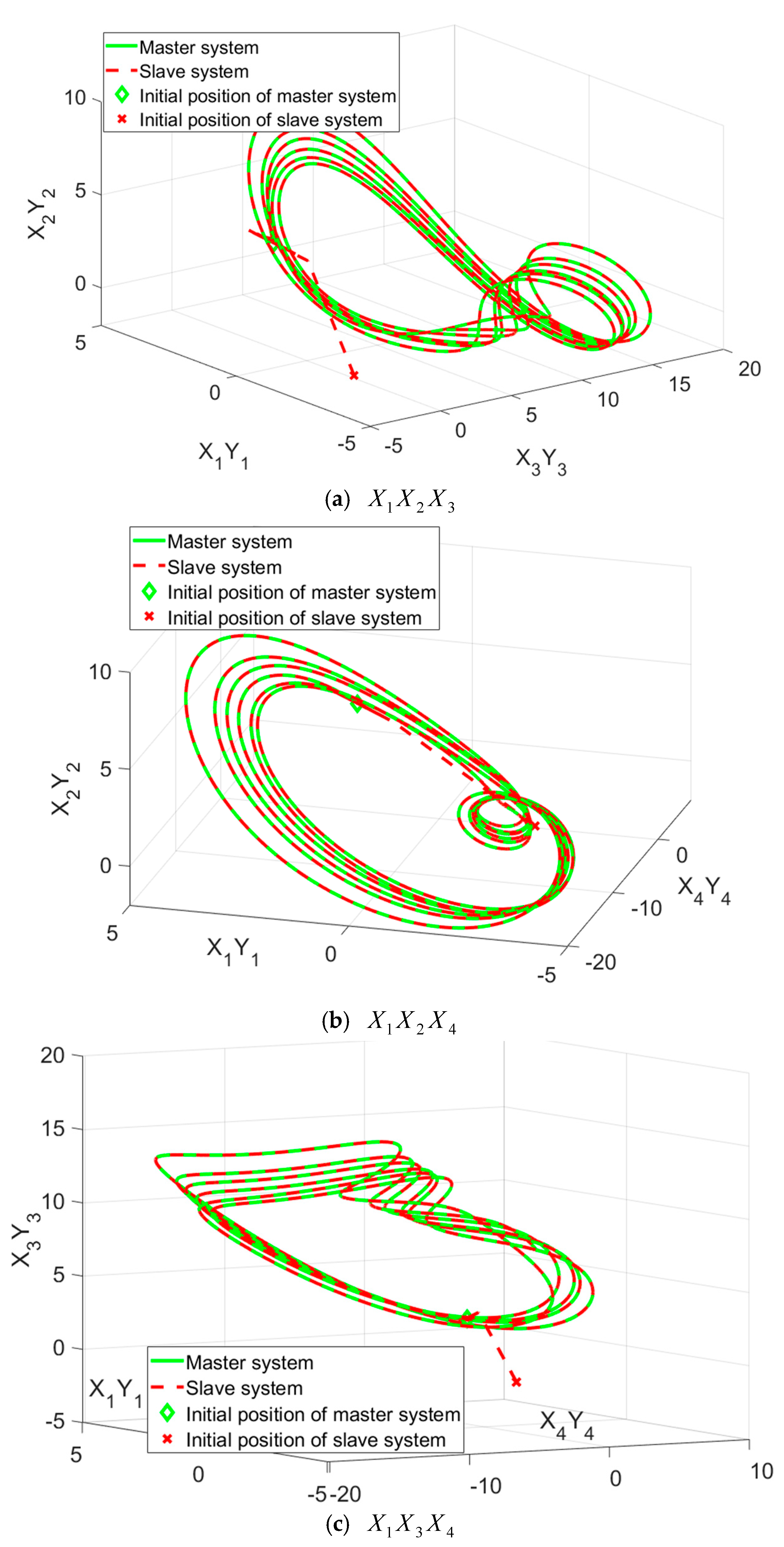
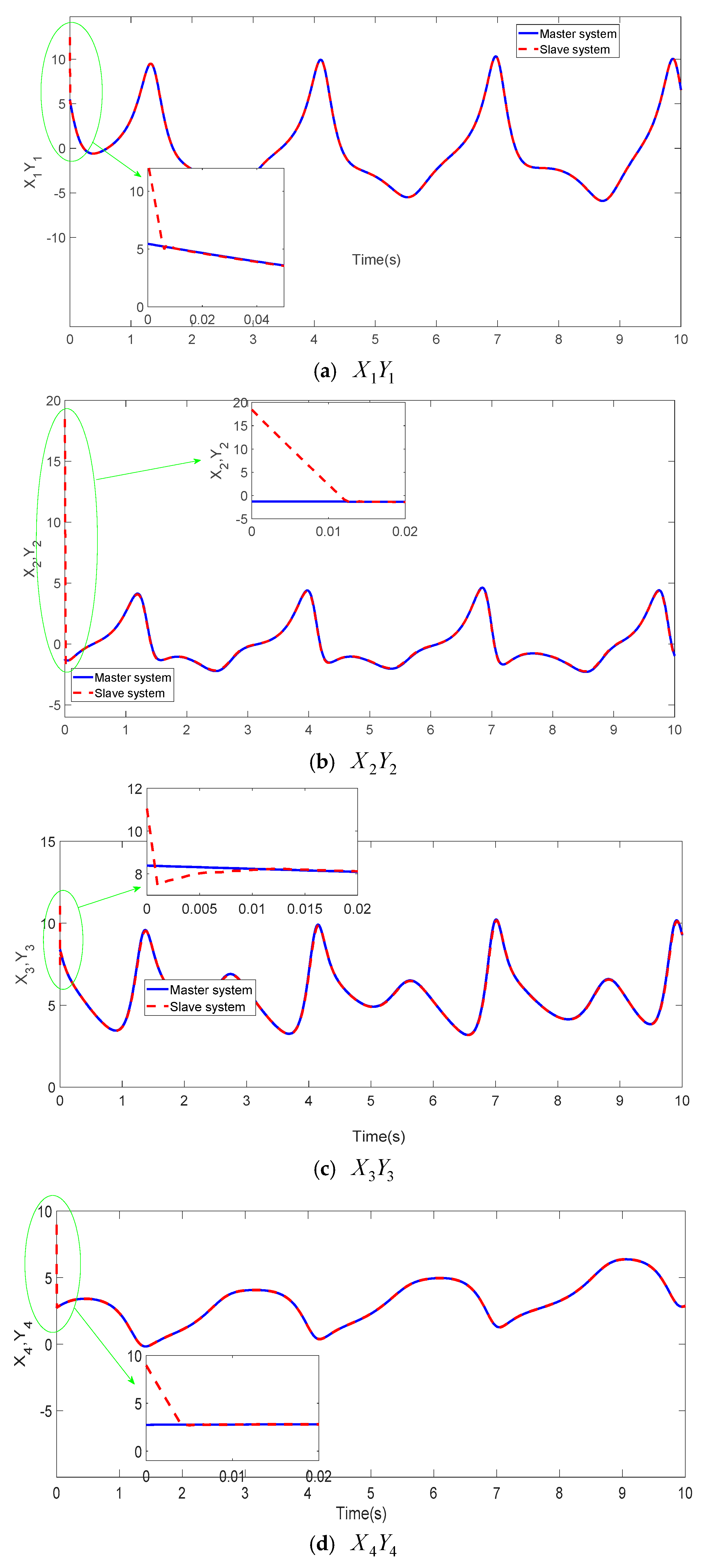
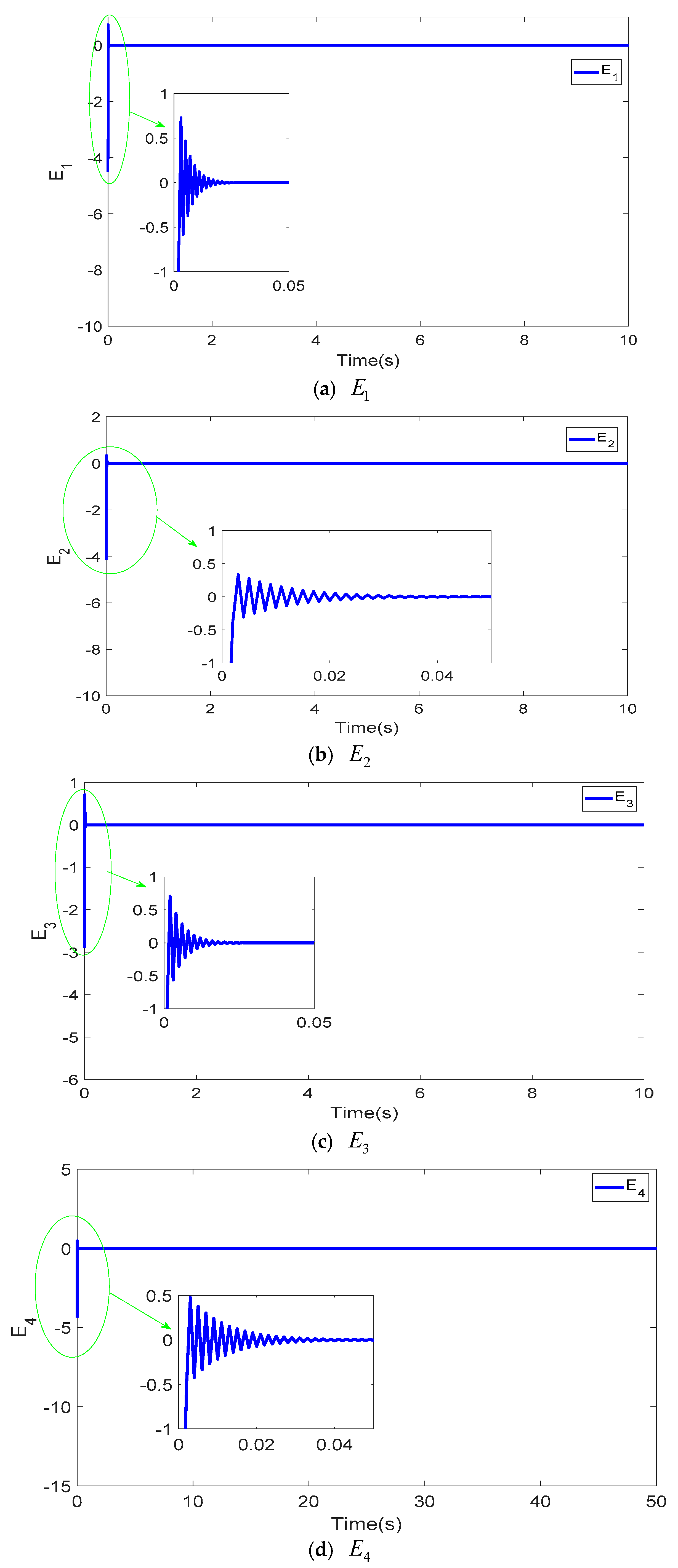
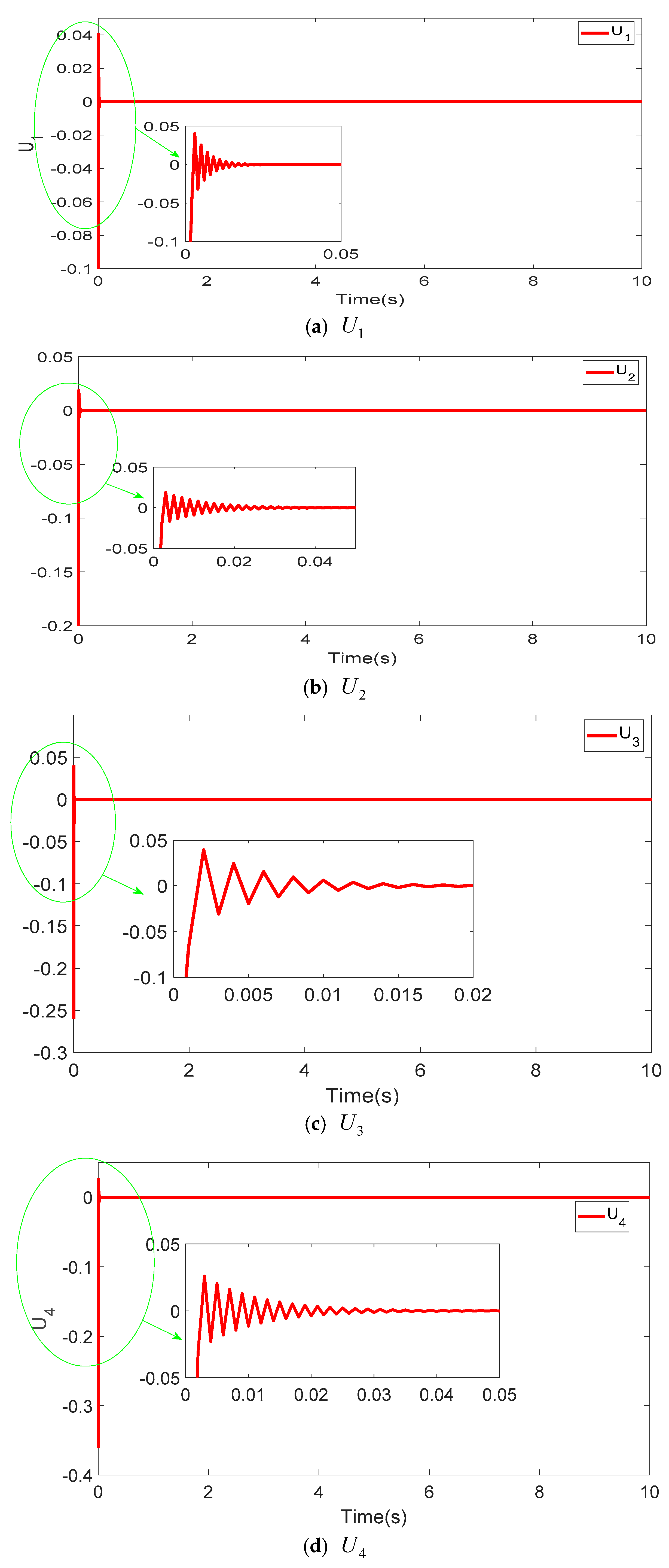
Figure 3 showcases the projection views of the synchronized states in the four-dimensional hyper-chaotic system using the TFWBCC approach. In Figure 4, the comparative analysis of state trajectories between the master and slave systems under the proposed TFWBCC methodology is illustrated. Figure 5 highlights the tracking error evolution, while Figure 6 visualizes the applied control inputs. The simulation results confirm that the proposed strategy successfully achieves synchronization with minimal tracking deviations.

Notably, the TFWBCC method significantly reduces the average RMSE, attaining the lowest error value among all compared techniques (see

Table 5. Evaluating the RMSE performance of TFWBCC against alternative approaches.

Method	RMSE1	RMSE2	RMSE3	RMSE4	Average_RMSE	Computation Time (s)
CMAC [32]	0.0505	0.0441	0.0267	0.0576	0.0445	0.00013
RCMAC [35]	0.0477	0.0425	0.0256	0.0548	0.0427	0.00014
TSKCMAC [13]	0.0479	0.0418	0.0252	0.0535	0.0418	0.00017
BELC [13]	0.0454	0.04049	0.0243	0.0511	0.0403	0.00029
The proposed TFWBCC	0.0277	0.0236	0.0118	0.0258	0.0222	0.00074

). However, due to its complex structure, the computational cost is higher. This trade-off is reasonable, as improved synchronization accuracy generally comes at the expense of increased processing demands. Specifically, the average RMSE of TFWBCC is reduced by a factor of 2.004 compared to the CMAC [32] method, 1.923 times compared to RCMAC [35], 1.8829 times compared to TSKCMAC [13], and 1.8153 times compared to BELC [13]. Additionally, the computation time of the TFWBCC approach is 5.6923 times lower than that of CMAC [32], 5.2857 times lower than RCMAC [35], and 4.3529 times lower than BELC [13].

5. The Application of 4D Master–Slave Chaotic Synchronization for Medical Image Encryption

The following outlines the image security algorithm:

Step 1: The original medical image undergoes a sorting process based on a dual-number scheme [13,41]

$$\mathrm{I}=\left[I_1,I_2,I_3\dots , I_{m\ast n}\right]$$

(58)

where m and n are the length size and width size of the original image, respectively.

Step 2: Synchronize the master and the slave system.

Step 3: After the synchronization, discrete the master system of the chaotic 4D system

$$\left\{\mathit{B}(j), j=1,2\dots ,p\times q\right\}$$

(59)

where j = 1, 2, … p × q represents the index of the j-th iteration within the chaotic system’s progression.

Step 4: The initial step involves thoroughly preprocessing the decimal value as follows:

$$\mathit{C}=\mathrm{round}(\mathrm{mod}((\mathrm{abs}(c_m(j))-\mathrm{floor}(\mathrm{abs}(c_m(j)))\times {10}^8,256))$$

(60)

where round(x) approximates x to the nearest whole number, mod(x, y) computes the remainder when x is divided by y, abs(x) determines the absolute magnitude of x, and floor(x) rounds x down to the nearest integer that is less than or equal to x.

Step 5: The process of image encryption is integrated with the primary chaotic system through the application of the XOR logical operation, as described below

$$G=\mathrm{de}2\mathrm{bi}(I)\otimes \mathrm{de}2\mathrm{bi}(C)$$

(61)

here, de2bi(.) transforms a decimal number into its binary equivalent, while ⊕ represents the logical XOR operation.

Step 6: Convert the binary representation of G into decimal form, then reorganize $X=\left[X_1,X_2 \dots , X_{p\times q}\right]$ to generate the encrypted image.

Step 7: Decryption Procedure.

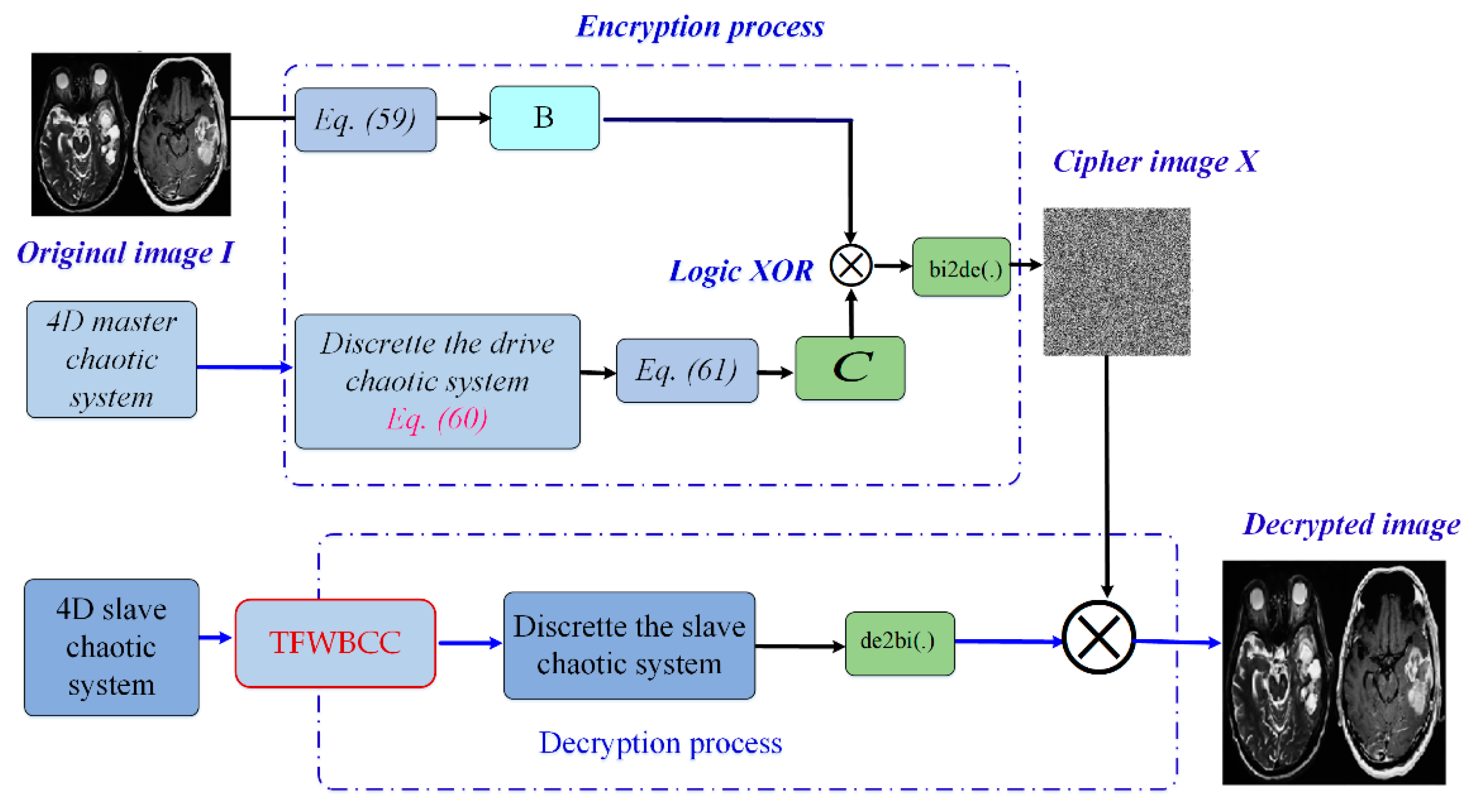
The decryption method reverses the encryption steps, with the key difference being that the master chaotic time series is substituted by the corresponding slave chaotic time series. The structure of the medical image encryption using master–slave chaotic synchronization is presented in Figure 7.

Some statistical analyses are performed to validate the proposed algorithm, such as histogram analysis and entropy analysis and NIST-SP800-22 test.

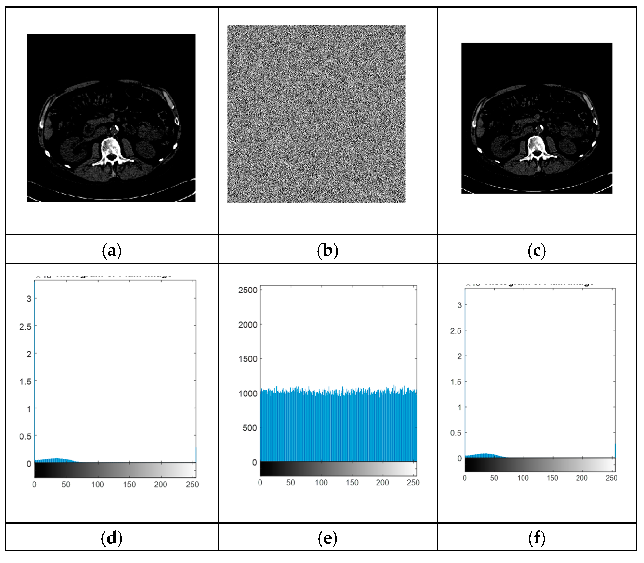
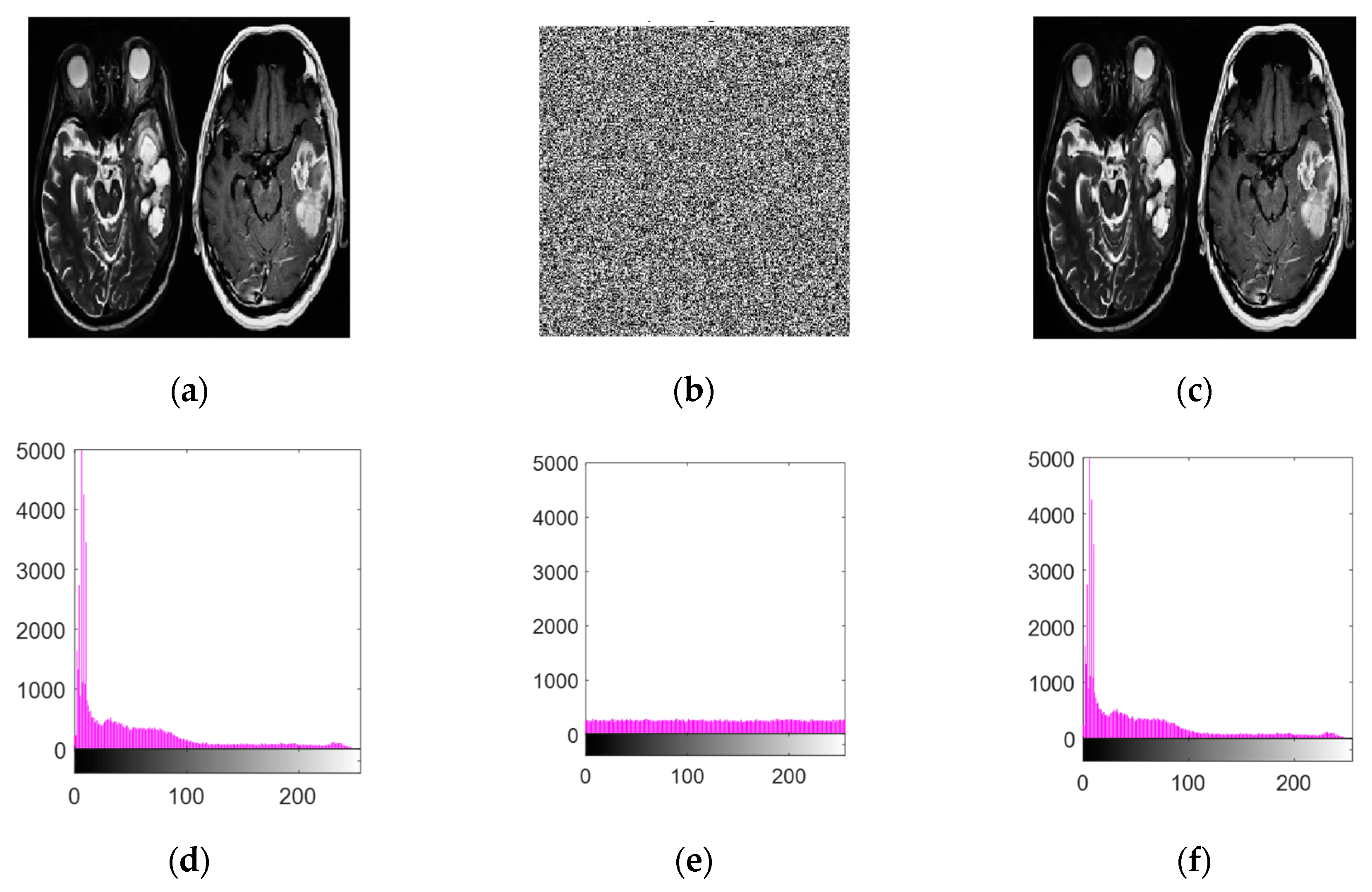
5.1. Histogram Examination

A histogram represents the pixel distribution within an image. To ensure security, the encrypted image must exhibit a distinct statistical distribution compared to the original plain image (refer to Figure 8 and Figure 9).

5.2. Entropy

Entropy quantifies the dispersion of grayscale values within an image. A uniform distribution results in a higher entropy value, reaching a theoretical maximum of 8. The entropy calculation is defined as follows:

$$\mathrm{E}({\zeta }_j)={\displaystyle \sum _{j=0}^{2^N-1}P({\zeta }_j){\log }_2}{\displaystyle \frac{1}{P({\zeta }_j)}}$$

(62)

where 2^N represents the total number of states in the information source, while $\mathrm{E}({\zeta }_j)$ denotes the probability of occurrence for the symbol ${\zeta }_j$. An ideally random image, R, exhibits a uniform pixel intensity distribution within the range [0, 255], implying that the probability $P({\zeta }_j)$ is equal to 1/2561/2561/256 for every j within [0, 255].

The entropy of the original image and the scrambled image is described in

Table 6. Entropy of the cipher image.

Method	Entropy of Cipher Image Lung	Entropy of Cipher Image Ruptured Brain
Method TSKCMAC [13]	7.9865	7.9851
Method TS Fuzzy [14]	7.9866	7.9852
Proposed method	7.968	7.9971

. The different values between the original and the brain show that our method works well. Table 6 shows the entropy of the scrambled images of our method compared to other methods. It can be seen that our method achieves a value close to 8, namely 7.9988 for the scrambled image lung and 7.9967 for the scrambled image ruptured brain. Our method gives the highest value among all methods. This shows that the content of the image is secure when there is an attack on the image information.

5.3. NIST SP800-22 Test

Referring to [42], the randomness of output sequences is evaluated using the National Institute of Standards and Technology (NIST) SP800-22 test suite. This standard includes 15 distinct subtests, each producing a p-value. To be considered random, the resulting p-value for each subtest must lie between 0.01 and 1.

Table 7. Analysis results of the NIST evaluation for the scrambled brain image.

Statistical Test	p-Value	Results
Overlapping templates	0.1485	The evaluation confirmed that the shuffled image met the required criteria, as all 15 subtests produced p-values falling within the acceptable threshold of 0.01 to 1.
Rank	0.0416
Serial p-value 2	0.2351
Random-excursions	0.2328
Linear complexity	0.2246
Longest run	0.0467
Random-excursions variant	0.3578
Discrete Fourier transform	0.3368
Serial p-value 1	0.3658
Approximate Entropy	0.3285
Frequency	0.249
Cumulative sums reserve	0.0419
Cumulative sums forward	0.0314
Runs	0.8358
Universal	0.5238

presents the assessment results for a 100-bit sample derived from 262,144 (512 × 512) bits of the encrypted “Brain Image”. The findings indicate that all p-values from the 15 subtests fall within the permissible range of 0–1, demonstrating that the encrypted image’s binary sequences successfully meet the randomness criteria. Consequently, the encryption effectively ensures pixel-level randomness.

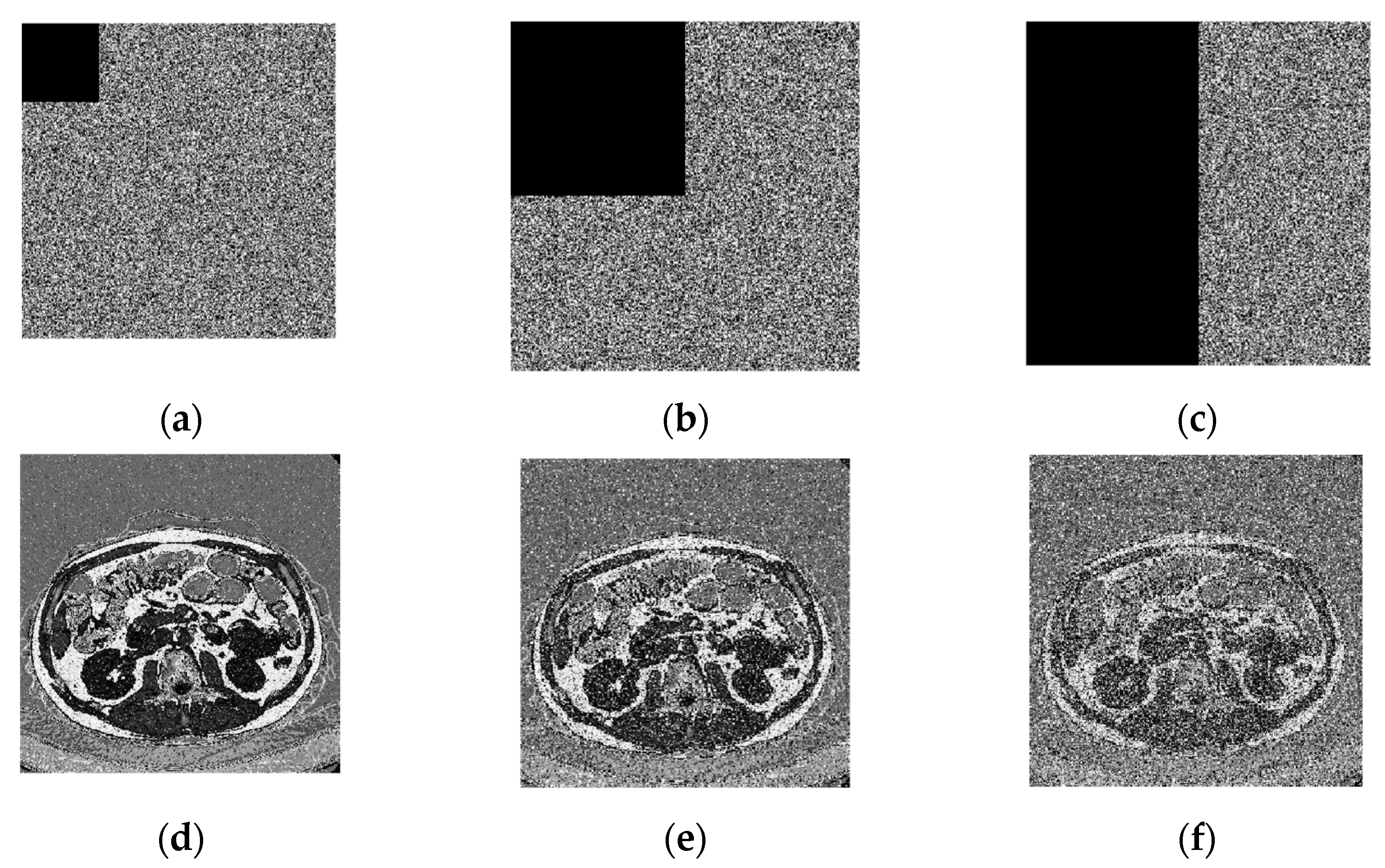
5.4. Cropping Attack Analysis

Our approach effectively handles data loss caused by cropping attacks. Figure 10 a,c,e displays scrambled images with varying levels of data removal—specifically, 1/16, 1/4, and 1/2 of the original content. Correspondingly, Figure 10b,d,f showcase the reconstructed images after decryption. The results indicate that our technique successfully recovers missing data. A comparative analysis in

Table 8. Quantitative results of cropping attacks using our method.

Lung Image 512 × 512	Average of PSNR (Original-Decrypted Images) (dB)
	TSKCMAC [13]	Our Method
1/16 data loss	10.2347	10.7549
1/4 data loss	6.2542	6.6141
1/2 data loss	5.2573	5.69453

demonstrates that our method achieves a higher PSNR value, validating its superior ability to reconstruct images even in the presence of data loss.

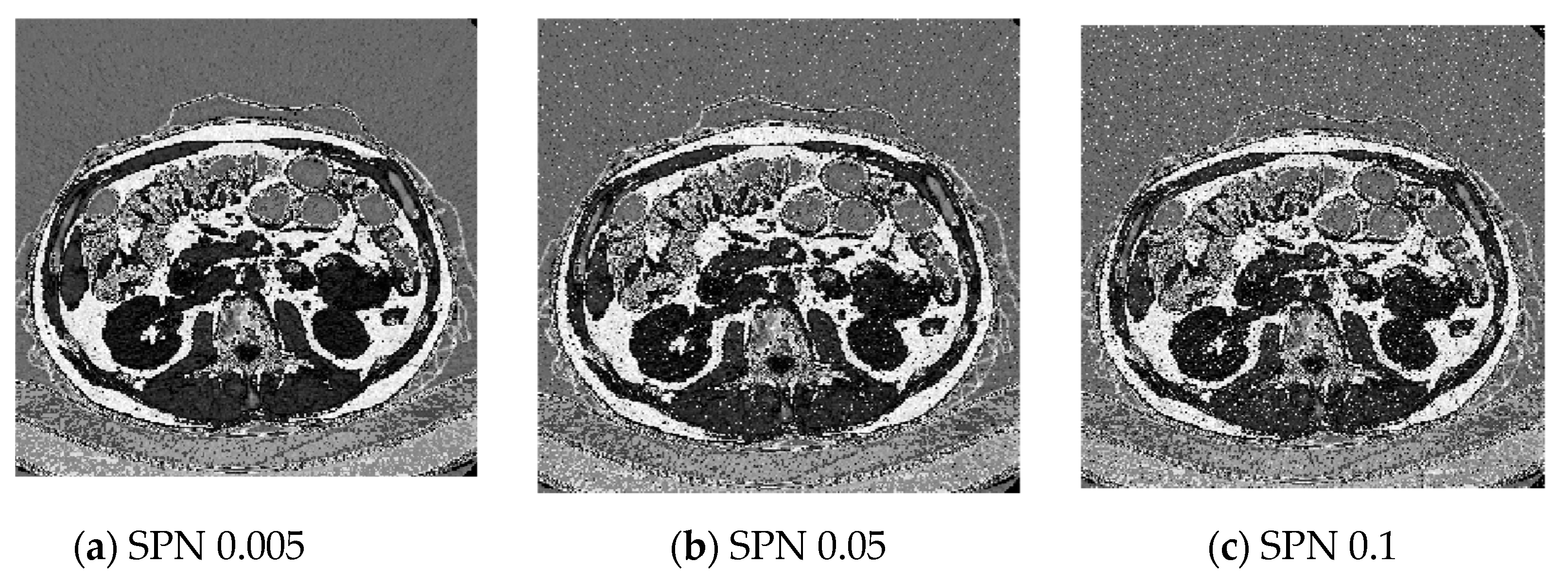
5.5. Image with Noise Analysis

To evaluate the effectiveness of the suggested approach, an image with adjustable noise parameters—both mean and variance—is utilized. This allows for an assessment of how varying levels of degradation impact on the method’s ability to encode the image while minimizing data loss. In this analysis, a lung image serves as the benchmark for testing the proposed technique. Figure 11 presents the encoded image subjected to Salt and Pepper Noise (SPN) with noise variances of 0.005, 0.05, and 0.1. The corresponding PSNR values, which are detailed in

Table 9. Image with difference noise addition.

Type of Noise	Variances	PSNR (Original-Decrypted Images) (dB)
Salt and pepper	0.005	5.886591
	0.05	5.890404
	0.1	5.836653

, indicate that (1) our encoding algorithm demonstrates significant robustness against SPN, maintaining PSNR values above 5.8 dB, and (2) the reconstructed images retain superior visual quality. These results confirm the method’s strong resistance to noise-induced distortions.

6. Conclusions

This research introduces a novel synchronization strategy for a four-dimensional hyper-jerk hyper-chaotic system. To accomplish this, adaptive parameter laws are formulated using a hybrid neural framework that combines TFWBC and TFWCC. The Lyapunov stability theorem is employed to establish online learning rules, ensuring both stability and system convergence. The proposed control mechanism effectively synchronizes the 4D master–slave hyper-jerk hyper-chaotic system with high precision. Additionally, the innovative TFWBCC approach is utilized to achieve synchronization of the chaotic states within the 4D Lorenz system. Furthermore, it is highlighted that this method can be applied to enhance the secure transmission of medical images. Simulation outcomes confirm the robustness and efficiency of the proposed control and encryption/decryption techniques. Statistical analyses further validate that the encryption/decryption approach ensures a high level of security.

Future advancements will first focus on adapting the proposed approach for hardware implementation, along with the development of a novel optimization algorithm, specifically an improved sparrow swarm optimization, will be implemented to improve the performance of the TFWBCC. In this study, we proposed a novel method for medical image encryption, demonstrating its effectiveness in ensuring data security and privacy. While the primary focus has been on medical imaging, the proposed approach holds significant potential for broader applications. Future studies could also explore its adaptation to other domains, such as secure communication systems, IoT device data encryption, and financial data protection. Investigating these avenues would further validate the versatility and scalability of the method, addressing critical security challenges across diverse fields. We believe these explorations will open new research directions and enhance the practical impact of the proposed framework.

References

1. Alber, D.A.; Yang, Z.; Alyakin, A.; Yang, E.; Rai, S.; Valliani, A.A.; Zhang, J.; Rosenbaum, G.R.; Amend-Thomas, A.K.; Kurland, D.B.; et al. Medical large language models are vulnerable to data-poisoning attacks. Nat. Med. 2025, 31, 618–626. [Google Scholar] [CrossRef]
2. Wang, W.; Yan, D.; Wu, X.; He, W.; Chen, Z.; Yuan, X.; Li, L. Low-light image enhancement based on virtual exposure. Signal Process. Image Commun. 2023, 118, 117016. [Google Scholar] [CrossRef]
3. An, X.; Du, L.; Jiang, F.; Zhang, Y.; Deng, Z.; Kurths, J. A few-shot identification method for stochastic dynamical systems based on residual multipeaks adaptive sampling. Chaos Interdiscip. J. Nonlinear Sci. 2024, 34, 073118. [Google Scholar] [CrossRef]
4. Polson, L.A.; Fedrigo, R.; Li, C.; Sabouri, M.; Dzikunu, O.; Ahamed, S.; Karakatsanis, N.; Kurkowska, S.; Sheikhzadeh, P.; Esquinas, P.; et al. PyTomography: A python library for medical image reconstruction. SoftwareX 2025, 29, 102020. [Google Scholar] [CrossRef]
5. Lu, S.Y.; Zhu, Z.; Tang, Y.; Zhang, X.; Liu, X. CTBViT: A novel ViT for tuberculosis classification with efficient block and randomized classifier. Biomed. Signal Process. Control 2025, 100, 106981. [Google Scholar] [CrossRef]
6. Cai, L.; Fang, H.; Xu, N.; Ren, B. Counterfactual Causal-Effect Intervention for Interpretable Medical Visual Question Answering. IEEE Trans. Med. Imaging 2024, 43, 4430–4441. [Google Scholar] [CrossRef]
7. Liu, X.; Yang, J. A novel multi-layer image encryption algorithm based on 2D drop-wave function. Nonlinear Dyn. 2025, 113, 1775–1797. [Google Scholar] [CrossRef]
8. Han, X.; Li, Y.; Liu, W.; Chen, X.; Song, Z.; Wang, X.; Deng, Y.; Tang, X.; Jiang, Z. The Applications of Magnetic Particle Imaging: From Cell to Body. Diagnostics 2020, 10, 800. [Google Scholar] [CrossRef] [PubMed]
9. Bing, P.; Liu, W.; Zhai, Z.; Li, J.; Guo, Z.; Xiang, Y.; He, B.; Zhu, L. A novel approach for denoising electrocardiogram signals to detect cardiovascular diseases using an efficient hybrid scheme. Front. Cardiovasc. Med. 2024, 11, 1277123. [Google Scholar] [CrossRef] [PubMed]
10. Lai, Q.; Hua, H. Secure medical image encryption scheme for Healthcare IoT using novel hyperchaotic map and DNA cubes. Expert Syst. Appl. 2025, 264, 125854. [Google Scholar] [CrossRef]
11. Wang, Y.; Xu, Y.; Song, J.; Liu, X.; Liu, S.; Yang, N.; Wang, L.; Liu, Y.; Zhao, Y.; Zhou, W.; et al. Tumor Cell-Targeting and Tumor Microenvironment–Responsive Nanoplatforms for the Multimodal Imaging-Guided Photodynamic/Photothermal/Chemodynamic Treatment of Cervical Cancer. Int. J. Nanomed. 2024, 19, 5837–5858. [Google Scholar] [CrossRef] [PubMed]
12. Chu, L.; Su, Y.; Zan, X.; Lin, W.; Yao, X.; Xu, P.; Liu, W. A Deniable Encryption Method for Modulation-Based DNA Storage. Interdiscip. Sci. Comput. Life Sci. 2024, 16, 872–881. [Google Scholar] [CrossRef]
13. Lin, C.-M.; Pham, D.-H.; Huynh, T.-T. Encryption and decryption of audio signal and image secure communications using chaotic system synchronization control by TSK fuzzy brain emotional learning controllers. IEEE Trans. Cybern. 2021, 52, 13684–13698. [Google Scholar] [CrossRef] [PubMed]
14. Giap, V.N.; Pham, D.H.; Lin, C.-M.; Trinh, M.H.; Le, M.C.; Nguyen, Q.D. Fractional Order T–S Fuzzy Chaotic Models for Secure EEG Signal via a Wireless Communication Protocol Using a Disturbance Observer and Sliding Mode Control Technique. Int. J. Fuzzy Syst. 2024, 26, 1897–1915. [Google Scholar] [CrossRef]
15. Aliabadi, F.; Majidi, M.-H.; Khorashadizadeh, S. Chaos synchronization using adaptive quantum neural networks and its application in secure communication and cryptography. Neural Comput. Appl. 2022, 34, 6521–6533. [Google Scholar] [CrossRef]
16. Zhang, S.; Peng, X.; Wang, X.; Chen, C.; Zeng, Z. A Novel Memristive Multiscroll Multistable Neural Network with Application to Secure Medical Image Communication. IEEE Trans. Circuits Syst. Video Technol. 2024, 35, 1774–1786. [Google Scholar] [CrossRef]
17. Katsikis, V.N.; Stanimirović, P.S.; Mourtas, S.D.; Xiao, L.; Karabašević, D.; Stanujkić, D. Zeroing neural network with fuzzy parameter for computing pseudoinverse of arbitrary matrix. IEEE Trans. Fuzzy Syst. 2021, 30, 3426–3435. [Google Scholar] [CrossRef]
18. Zhu, G.; Ma, Y.; Hu, S. Event-Sampled Adaptive Fuzzy Control of MASS via Intermittent Position Data. IEEE Trans. Emerg. Top. Comput. Intell. 2025, 1–13. [Google Scholar] [CrossRef]
19. Luo, Y.; Huang, Y.; Yu, F.; Liang, D.; Lin, H. Adaptive Asymptotic Shape Synchronization of a Chaotic System with Applications for Image Encryption. Mathematics 2025, 13, 128. [Google Scholar] [CrossRef]
20. Liu, X.; Lv, H. Disturbance Observer-based Adaptive Synchronization of Heterogeneous Chaotic Systems with Uncertainties via DNA Strand Displacement. IEEE Trans. Comput. Biol. Bioinform. 2025, 22, 250–260. [Google Scholar] [CrossRef]
21. Li, K.; Liu, X. Fuzzy Adaptive Cooperative Prescribed Time Control for Nonlinear Vehicular Platoon Systems. IEEE Trans. Fuzzy Syst. 2025, 1–10. [Google Scholar] [CrossRef]
22. Yi, J.; Mao, J.; Zhang, H.; Chen, Y.; Liu, T.; Zeng, K.; Xie, H.; Wang, Y. Balancing Accuracy and Efficiency with a Multiscale Uncertainty-Aware Knowledge-Based Network for Transmission Line Inspection. IEEE Trans. Ind. Inform. 2025, 1–10. [Google Scholar] [CrossRef]
23. Dang, G.; Wang, D. Online Self-Learning Fuzzy Recurrent Stochastic Configuration Networks for Modeling Nonstationary Dynamics. IEEE Trans. Fuzzy Syst. 2025, 1–14. [Google Scholar] [CrossRef]
24. Fan, Q.; Ji, D. Identification and Convergence Analysis of Interval Type-2 Takagi-Sugeno-Kang Fuzzy Systems for High-Dimensional Classification Problems. IEEE Trans. Fuzzy Syst. 2025, 1–16. [Google Scholar] [CrossRef]
25. Li, Y.; Zhou, E.; Vong, C.-M.; Wang, S. Stacked Ensemble of Extremely Interpretable Takagi–Sugeno–Kang Fuzzy Classifiers for High-Dimensional Data. IEEE Trans. Syst. Man Cybern. Syst. 2025, 1–12. [Google Scholar] [CrossRef]
26. Shirgir, S.; Farahmand-Tabar, S. An enhanced optimum design of a Takagi-Sugeno-Kang fuzzy inference system for seismic response prediction of bridges. Expert Syst. Appl. 2025, 266, 126096. [Google Scholar] [CrossRef]
27. Liu, C.-L.; Chang, Y.-H. Learning from imbalanced data with deep density hybrid sampling. IEEE Trans. Syst. Man Cybern. Syst. 2022, 52, 7065–7077. [Google Scholar] [CrossRef]
28. Liu, A.; Zhao, H.; Song, T.; Liu, Z.; Wang, H.; Sun, D. Adaptive control of manipulator based on neural network. Neural Comput. Appl. 2021, 33, 4077–4085. [Google Scholar] [CrossRef]
29. Liang, H.; Liu, G.; Zhang, H.; Huang, T. Neural-network-based event-triggered adaptive control of nonaffine nonlinear multiagent systems with dynamic uncertainties. IEEE Trans. Neural Netw. Learn. Syst. 2020, 32, 2239–2250. [Google Scholar] [CrossRef] [PubMed]
30. Murugan, S.; Anh, L.H.; Le, T.-L. Non-linear Control System Using Function-Link Fuzzy Brain Emotional Controller. Int. J. Fuzzy Syst. 2024, 26, 434–448. [Google Scholar] [CrossRef]
31. Chao, F.; Zhou, D.; Lin, C.M.; Yang, L.; Zhou, C.; Shang, C. Type-2 Fuzzy Hybrid Controller Network for Robotic Systems. IEEE Trans Cybern 2020, 50, 3778–3792. [Google Scholar] [CrossRef] [PubMed]
32. Lin, F.-J.; Sun, I.-F.; Yang, K.-J.; Chang, J.-K. Recurrent fuzzy neural cerebellar model articulation network fault-tolerant control of six-phase permanent magnet synchronous motor position servo drive. IEEE Trans. Fuzzy Syst. 2015, 24, 153–167. [Google Scholar] [CrossRef]
33. Yu, Y.; Si, X.; Hu, C.; Zhang, J. A review of recurrent neural networks: LSTM cells and network architectures. Neural Comput. 2019, 31, 1235–1270. [Google Scholar] [CrossRef] [PubMed]
34. Sherstinsky, A. Fundamentals of recurrent neural network (RNN) and long short-term memory (LSTM) network. Phys. D Nonlinear Phenom. 2020, 404, 132306. [Google Scholar] [CrossRef]
35. Fan, R.; Li, Y. An adaptive fuzzy trajectory tracking control via improved cerebellar model articulation controller for electro-hydraulic shovel. IEEE/ASME Trans. Mechatron. 2021, 26, 2870–2880. [Google Scholar] [CrossRef]
36. Hou, S.; Fei, J.; Chen, C.; Chu, Y. Finite-time adaptive fuzzy-neural-network control of active power filter. IEEE Trans. Power Electron. 2019, 34, 10298–10313. [Google Scholar] [CrossRef]
37. Zheng, K.; Zhang, Q.; Hu, Y.; Wu, B. Design of fuzzy system-fuzzy neural network-backstepping control for complex robot system. Inf. Sci. 2021, 546, 1230–1255. [Google Scholar] [CrossRef]
38. Pham, V.-T.; Vaidyanathan, S.; Volos, C.; Wang, X.; Hoang, D.V. A hyperjerk memristive system with hidden attractors. In Advances in Memristors, Memristive Devices and Systems; Springer: Berlin/Heidelberg, Germany, 2017; pp. 59–80. [Google Scholar]
39. Huynh, T.-T.; Lin, C.-M.; Pham, T.-T.T.; Cho, H.-Y.; Le, T.-L. A modified function-link fuzzy cerebellar model articulation controller using a PI-type learning algorithm for nonlinear system synchronization and control. Chaos Solitons Fractals 2019, 118, 65–82. [Google Scholar] [CrossRef]
40. Utkin, V.I. Sliding Modes in Control and Optimization; Springer Science & Business Media: Berlin/Heidelberg, Germany, 2013. [Google Scholar]
41. Wu, Y.; Zhang, L.; Berretti, S.; Wan, S. Medical image encryption by content-aware DNA computing for secure healthcare. IEEE Trans. Ind. Inform. 2022, 19, 2089–2098. [Google Scholar] [CrossRef]
42. Bassham, L.E., III; Rukhin, A.L.; Soto, J.; Nechvatal, J.R.; Smid, M.E.; Barker, E.B.; Leigh, S.D.; Levenson, M.; Vangel, M.; Heckert, N.A.; et al. A Statistical Test Suite for Random and Pseudorandom Number Generators for Cryptographic Applications; SP 800-22 Rev. 1a; National Institute of Standards & Technology: Gaithersburg, MD, USA, 2010. [Google Scholar]
Figure 3. Visualization of a four-dimensional chaotic system in three-dimensional space.
Mathematics 13 00923 g003
Figure 4. Utilizing TFWBCC for monitoring the path of each dimension in a four-dimensional chaotic framework.
Mathematics 13 00923 g004
Figure 5. Application of TFWBCC to analyze the deviance signals across all dimensions in a four-dimensional chaotic model.
Mathematics 13 00923 g005
Figure 6. Employing TFWBCC to regulate the command signals for every dimension in a four-dimensional chaotic system.
Mathematics 13 00923 g006
Figure 7. The structure of the medical image encryption using 4D master–slave chaotic synchronization.
Mathematics 13 00923 g007
Figure 8. (a) The initial brain image, (b) its encrypted counterpart, (c) the decrypted version after restoration, (d) the pixel intensity distribution of the original image, (e) the histogram analysis of the encrypted image, and (f) the histogram corresponding to the decrypted image.
Mathematics 13 00923 g008
Figure 9. (a) Unaltered brain scan, (b) its encrypted transformation, (c) the restored image post-decryption, (d) intensity distribution analysis of the original image, (e) histogram visualization of the encrypted version, and (f) histogram representation of the decrypted image.
Mathematics 13 00923 g009
Figure 10. The result of brain image cropping attack, (a) 1/16 data loss, (b) 1/4 data loss, (c) 1/2 data loss, (d) decrypted image of (a), (e) decrypted image of (b), (f) decrypted image of (c).
Mathematics 13 00923 g010
Figure 11. Decrypted images under different noises with different variances.
Mathematics 13 00923 g011