A CFD-Based Correction for Ship Mass and Longitudinal Center of Gravity to Improve Resistance Simulation

Abstract

In this study, a correction procedure for ship mass and its longitudinal location of center of gravity suitable for a simulation environment is proposed in OpenFOAM v6.0. The concept is implemented ensuring static equilibrium and an approximately zero-pitch moment on the ship before the simulation. The viscous flow field around the ship in calm water is simulated using the VOF (Volume of Fluid) free surface two-phase and SST (Shear Stress Transport) k–ω turbulence models. Using static mesh, the resistance error of medium and fine grids is 4%, on average, against the experimental value. As the sinkage and trim are predicted using dynamic mesh, the increasing ship’s resistance causes larger errors, except for the container ship. Through the proposed correction, the ship’s vertical motions are significantly improved, and the resistance error decreases for the dynamic simulation. For the container ship, the error of resistance and motion achieved is less than 1%. The sinkage and trim errors improve tremendously for the tanker and bulk carrier, and the resistance errors are reduced slightly, by less than 3%. In the end, the detailed flow field is analyzed, as well as the ship wave-making pattern and the nominal wake velocity distribution, and these are compared with the measurement data available. The characteristics of the flow phenomena are successfully modeled. The resistance value for each hull form satisfies the requirement of Verification and Validation, and the uncertainty values are estimated.

1. Introduction

Based on the need for research and development in industry, academic study and financial consideration, designers, scientists and engineers have been increasingly relying on simulation tools for all kinds of analysis, such as CFD (Computational Fluid Dynamics). The objective of the presented work is to perform a ship resistance test in calm water using CFD for three open-source hull forms: KVLCC2 (KRISO Very Large Crude Carrier 2), KCS (KRISO Container Ship) and JBC (Japan Bulk Carrier). For global value prediction, steady total resistance, sinkage and trim are considered. A detailed flow field is also analyzed, including ship wave pattern, i.e., free surface elevation of ship wave-making, and ship wake velocity field, i.e., nominal wake distribution or boundary layer pattern on the propeller plane. V & V (Verification and Validation) is conducted to ensure our CFD method is reliable and convincing within acceptable uncertainty and error. In addition, it is expected that CFD will be used to assist our towing tank experiment in the future, and the foundation of further CFD applications in ship hydrodynamics will be established.

The hull forms of KCS and KVLCC2 have existed for a long time and have been investigated by many researchers. Many experimental data and simulation analyses can be found. Both hull forms were published and studied firstly by Kim et al. [1]. The towing tank experimental data for bare hull resistance, the nominal wake profile (using pitot tubes), and the wave-making patterns of both ship models were provided. Since then, the hull forms have been selected as the benchmark ships for test cases at many international conference series, for example, the Workshop on CFD in Ship Hydrodynamics: Gothenburg 2010 (G2010), Tokyo 2015 (T2015) and Wageningen 2025 (W2025). These focused on ship vertical motions, resistance and propulsion in calm water, as well as their seakeeping performance. Also, SIMMAN 2008, 2014, and 2021 were Workshops on Verification and Validation of Ship Manoeuvring Simulation Methods. The first appearance of JBC was in T2015. KCS and JBC will be the study cases for breaking waves and turbulence, respectively, in W2025.

The hull form of KCS features a transom stern with a wide and flat wet area facing downward and a long bulbous bow protruding forward. Kim et al. [1] revealed the KCS transom stern would result in an unsteady and complicated wave pattern in steady calm water conditions. Jasak et al. [2] pointed out that these phenomena cause a pressure distribution fluctuation on the ship’s stern surface and further influence the residual resistance fluctuation. In that study, a cluster computer with 8 × 8 cores of CPUs and OpenFOAM was used to simulate the resistance test for KCS and a combatant. For KCS, the total grid number was 1.13 M, 2.04 M and 4.06 M (M: million), corresponding to y⁺ = 66, 32, and 32, respectively. The total resistance errors were 0.38%, 1.18 and 1.91%. Jasak [3] claimed Naval Hydro Pack could provide converged and accurate calm-water resistance within 30 min if small y⁺ and grid quality were not requested. Using EBM (the embedded boundary method) in OpenFOAM, Gatin et al. [4] conducted a complete V & V analysis for KCS in calm water for six ship speeds corresponding to Froude numbers Fr = 0.108, 0.152, 0.195, 0.227, 0.260 and 0.282. A numerical uncertainty of 3.5%, 2.6% and 3.4% was reported in the verification results for the bare hull resistance, sinkage and trim, respectively. The resistance and sinkage prediction achieved monotonic convergence, but the trim raised large error in low Fr because of the too small value. The validation concluded that the average error of the resistance was less than 2.5% and only 0.4% for Fr = 0.26. Excluding the data for low Fr, which had the problem of being too small in value, the average error was 3.5 and 6.2% for sinkage and trim.

Many CFD resistance tests for KVLCC2 were combined in ship seakeeping and maneuvering studies. In Sadat-Hosseini et al. [5], the experimental data for KVLCC2 were provided by three towing tanks: Osaka University (OU), INEAN (Marine Technology Research Institute, Italy) and NTNU (Norwegian University of Science and Technology). CFDSHIP-IOWA estimated the calm-water resistance, sinkage and trim with over-predicted 7.8%, over-predicted 2.2% and under-predicted 4% against OU data. For V & V, one wavelength condition was analyzed with three different grid sizes and three different time steps. The grid refinement and time step ratio were both $\sqrt{2}$. Consequently, except for the mean pitch value, which was the oscillatory convergence, the other values reached monotonic convergence, including the mean value and the amplitude of the heave motion, pitch amplitude and mean resistance. Total uncertainty was only 3.46% of the result of the 4.6 M grids and the non-dimensional time step 0.015. Following [5], Wu et al. [6] found that, in long waves, due to large ship vertical motion, the bilge vortex and boundary layer profile move vertically and periodically with a high frequency component. The average nominal wake factor would be higher than the calm-water value. Islam and Akimoto [7] demonstrated that the code Ship_Motion predicted the trim well but slightly mis-predicted the sinkage at high ship speed. Increasing total grid number (from 2.98 M and 3.9 M to 5.56 M) and with better grid distribution, the calm-water resistance prediction was improved with monotonic convergence. However, at high ship speed, the resistance error increases slightly because the code cannot capture the hollow and hump of bow waves. Fureby et al. [8] applied RANS (Reynolds Averaged Navier–Stokes), LES (Large Eddy Simulation) and hybrid RANS-LES methods to investigate the flow field around KVLCCS at different drift angles. The 0° drift case was equivalent to the calm-water resistance test. The double-body model was utilized. For the total resistance, the under-predicted error was 5.8% for ReFRESCO (RANS, 12.5 M grids), 7.8% for EDGE (RANS-LES, 73 M grids) and 8.2% for OpenFOAM (LES, 121 M grids). EDGE using RANS with 73 M grids over-estimated by 3.9%. LES and RANS-LES showed more flow field details, especially the complicated vortex system. The axial velocity profiles in the nominal wake of the three methods all agreed acceptably with the experiment, but the LES result was closer.

In the T2015 conference, JBC was proposed for the first time with experimental data provided by several institutes. The flow field was measured using S-PIV (stereo-particle image velocimetry) in towing tanks. Meanwhile, to challenge this new test case, many simulations were presented at the conference. Hino et al. [9] drew the post-conference conclusion for all CFD predictions for JBC. To obtain an error of less than 4%, 10 M grids were required. For resistance, the mean absolute error was 2%, which was less than 5% mean validation uncertainty, i.e., overall CFD was validated for JBC cases. Mean sinkage absolute error was 4.7% and trim was 3.1%. Both errors were much improved from the G2010 cases. The resulting difference between the k-ε and k-ω turbulence models was below 2%. Both turbulence models also predicted the resistance better than more advanced models. CFD using a wall function predicted resistance better than it solved near-wall flow. However, only hybrid RANS-LES or LES could reproduce the turbulence kinetic energy distribution of the bilge vortex as measured in the experiment.

Bensow and van den Boogaard [10] implemented the PANS (Partially Averaged Navier–Stokes) method in the RANS solver in OpenFOAM. The transient flow field was simulated with PANS around a JBC with a double-body model. Along with the original k-ω turbulence model, another set of k-ω equations was required in PANS to solve unresolved turbulent kinetic energy and dissipation. The grid numbers were 14.7 M, 19.2 M and 31.7 M, with y⁺ fixed to 0.45. Even for the finest grid, the viscous resistance was under-predicted. The local flow details of PANS and RANS were similar. The bilge vortex strength still tended to be weak compared to the experimental flow field measurement and LES or DES (Detached Eddy Simulation). Nevertheless, the flow field results of PANS still provided more dynamic components, and even unsteadiness was over-predicted. Maasch et al. [11] proposed a detailed nominal wake analysis for JBC bare hull in calm water. A general purposed analysis tool named WAT (Wake Analysis Tool) was developed by inputting the CFD results. Five BSRA (British Ship Research Association) criteria were cited to determine the quality of ship wake. The CFD simulation was conducted using Star-CCM+ with an unstructured grid mixing with Cartesian cut-cell and prism. To adopt a wall function, the average y⁺ was about 35, and y⁺ remained less than 30 on the stern wet area. VOF was used for free surface modeling. The turbulence model was an SST (Shear Stress Transport) k-ω model with curvature correction. DFBI (Dynamic Fluid Body Interaction) was applied to predict sinkage and trim. The grid numbers were 1.36, 2.7 M and 6.87 M. The time step was 0.025 s to control, and the Courant number was around 1. C_T was verified and validated with 2–3% error higher than 1% experimental uncertainty. Sinkage and trim error were 2–4% and 4%.

Islam and Soares [12] compared two V & V theories in great detail for KCS, KVLCC2, JBC and DTC (Duisburg Test Case), for resistance, sinkage and trim obtained from an OpenFOAM simulation. It turned out that different V & V theories provided different outcomes, i.e., V & V results were case-specific. In addition, some large errors in the steady ship motions can be found in the results. The error of (C_T, sinkage, trim) was (−7.78%, −6.5, −65.6%) for KCS at Fr = 0.26, (−0.14%, −33.5%, −116.5%) for KCS at Fr = 0.195, (1.38%, −84.21%, −2.27%) for KVLCC2 at Fr = 0.142, (1.35%, −105.34%, 0%) for KVLCC2 at Fr = 0.119 and (−2.82%, −1677%, −1.11%) for JBC at Fr = 0.142. A negative value means over-prediction. The grid numbers listed here were 5.57 M, 3.54 M and 3.77 M for KCS, KVLCC2 and JBC. Refining the grid number to 10 M for KCS and JBC only reduced the C_T error.

The presented work proposes a correction procedure, “LCGM (Longitudinal Center of Gravity and Mass)”, to improve the vertical motion prediction of a CFD ship resistance test in calm water. The ship mass and the location of the ship’s center of gravity should be adjusted since the ship surface in CFD is discretized from the original geometry. For instance, using an n-sided polygon to approximate a circle will never form an exact circle but only approach a circle as n increases. The centroid of the polygon shifts depending on the arrangement and length of the sides. Some CFD software, such as REX [13] and CFDSHIP-IOWA [14], feature this function, but not for the original package of OpenFOAM v6.0. Thus, it is worth developing this procedure exclusively for further and future CFD application in ship hydrodynamics and ship engineering.

2. CFD Methods

2.1. Numerical Schemes

The analysis tool used in the presented work is the open source CFD code OpenFOAM (Open Source Field and Manipulation), version 6. The viscous flow field with air–water free surface modeling is simulated around the ship hull. The incompressible two-phase flow model, VOF (Volume of Fluid) [15,16], is utilized to solve the velocity, pressure field and free surface elevation around the ship hull. The turbulence model is the SST (Shear Stress Transport) k-ω model [17]. The velocity and pressure coupling is PIMPLE [18], which is an exclusive algorithm developed in OpenFOAM. It is a hybrid approach of PISO [19] (pressure implicit with splitting of operator) and SIMPLE [20] (Semi-Implicit Method for Pressure Linked Equations). SIMPLE is suitable for steady problems, and unsteady time accuracy is considered in PISO. PIMPLE consists of an inner and outer loop to ensure continuity is satisfied for the momentum corrector and predictor, respectively. The inner loop functions resemble PISO, and the outer loop operates like SIMPLE. Therefore, large time steps and a Courant number larger than 1 are allowed using PIMPLE. In addition, the VOF in OpenFOAM, i.e., interFoam solver, is only compatible with PIMPLE.

In static mesh simulation, only resistance and flow field are predicted. To predict sinkage and trim along with resistance and flow field, dynamic mesh is required. The linear and rotation displacement of ship motions are obtained by solving rigid body equations of motion with quaternions. In this study, only 2DOF (degree of freedom) is considered, i.e., heave and pitch corresponding to sinkage and trim in a ship resistance test. The equations of motions are solved using the Crank–Nicolson second-order time-integrator. Through the time integral of the solved acceleration, the ship moving displacement and velocity are calculated, and then the grid is deformed according to the solved displacement. The flow field and motion solver are coupled in inner iteration. The flow flux across the cell faces due to the grid deformation and moving velocity is considered in the finite volume method. Inner and outer distance are specified to distinguish three grid deformation regions. The grids (1) within the inner distance move with the ship without deformation, (2) behind the outer distance maintain static and neither move nor deform and (3) deform between the inner and outer distance, and a diffusion equation is solved to preserve grid quality.

The main numerical scheme to discretize the Navier–Stokes equations and the above-mentioned flow field models is the finite volume method. The temporal term is integrated using the first-order Euler method implicit with local time stepping for static mesh simulation. With the dynamic mesh, the first-order Euler method could be used with an automatic time step adjustment based on the global Courant number. The gradient term is computed by the first-order central difference method. The second-order upwind method is applied as the divergent term. The Laplacian term, and the value at the center point of a surface, are obtained with a linear interpolation. The gradient in the normal direction on a surface is calculated using the second-order explicit non-orthogonal correction.

2.2. Governing Equations

This section will discuss the fluid dynamics equations, which will be solved using the numerical methods summarized in Section 2.1. Equations (1) and (2) are for the mass and momentum conservation, respectively, i.e., the Navier–Stokes equations

$$\nabla ·\mathbf{U}=0,$$

(1)

$${\displaystyle \frac{\partial \rho \mathbf{U}}{\partial t}}+\nabla ·\rho \mathbf{U}\mathbf{U}-\nabla ·(\mu +{\mu }_t)\left(\nabla \mathbf{U}\right)-\nabla \mathbf{U}·\nabla (\mu +{\mu }_t)=-\nabla p-\mathbf{g}·\mathbf{X}\nabla \rho ,$$

(2)

$${\mu }_t=0.31\rho k/\max \left\{0.31\omega , \mathrm{t}\mathrm{a}\mathrm{n}\mathrm{h}\left[{\max \left[{\displaystyle \frac{2\sqrt{k}}{0.09\omega d}},{\displaystyle \frac{500\mu }{\rho \omega d^2}}\right]}^2\right]\right\},$$

(3)

where $\mathbf{U}$ = ($u\widehat{i}+v\widehat{j}+w\widehat{k}$): fluid velocity, t: time, $\rho$: density, p: pressure, $\mathbf{X}$ = $\left(x\widehat{i}+y\widehat{j}+z\widehat{k}\right)$: position vector and $\mathbf{g}$ = −9.81$\widehat{k}$ m/s. $\mu$ (fluid viscosity) + ${\mu }_t$ (turbulent viscosity) is the so-called effective dynamic viscosity. d is the distance between the field point and the nearest wall. $\widehat{i}, \widehat{j}, \widehat{k}$ are the unit vectors in the direction of the x, y, z axes of the Cartesian coordinate.

In the SST k-ω turbulence model [17], ${\mu }_t$ is provided via Equation (3) by solving k (turbulence kinetic energy) and ω (turbulence dissipation rate) in Equations (4) and (5)

$${\displaystyle \frac{\partial \left(\rho k\right)}{\partial t}}+\nabla \rho \mathbf{U}k=\widetilde{P_k}-0.09\rho k\omega +\nabla \left[\left({\mu +{\sigma }_k\mu }_t\right)\nabla k\right],$$

(4)

$${\displaystyle \frac{\partial \left(\rho \omega \right)}{\partial t}}+\nabla \rho \mathbf{U}\omega =\rho \left(\gamma {\mathbf{S}}^2-\beta {\omega }^2\right)+\nabla \left[\left({\mu +{\sigma }_{\omega }\mu }_t\right)\nabla \omega \right]+2(1-F){\displaystyle \frac{0.856\rho }{\omega }}\nabla k\nabla \omega ,$$

(5)

$${\left[{\sigma }_k {\sigma }_{\omega } \beta \gamma \right]}^T=F{\left[0.85 0.5 0.075 5/9\right]}^T+(1-F){\left[1.0 0.856 0.0828 0.44\right]}^T,$$

(6)

$$F=\tanh \left\{{\left\{\min \left[\max \left({\displaystyle \frac{\sqrt{k}}{0.09\omega d}},{\displaystyle \frac{500\mu }{\rho \omega d^2}}\right),{\displaystyle \frac{3.424k}{\max \left(\frac{1.712\rho \nabla k\nabla \omega }{\omega },{10}^{-10}\right)d^2}}\right]\right\}}^4\right\},$$

(7)

in which $\widetilde{P_k}$ is the production limiter, $\mathbf{S}$ the strain rate tensor and $\beta$ the coefficient of thermal expansion. The constants in Equations (4) and (5) are switched between the k-ε and k-ω models in Equation (6) for F = 0 and 1, respectively. Equation (7) indicates F = 0~1 is a hyperbolic tangent function to blend two models and transit between them smoothly. Consequently, the k-ω model is activated inside the boundary layer close to the wall, and the k-ε model is turned on near the free stream away from the wall.

In VOF, $\rho$ and $\mu$ in the equatoins, respectively, are composed of water (subscript w) and air (subscript a) through the volume fraction $\alpha$, as shown in Equations (8) and (9):

$$\rho ={\rho }_w\alpha +{\rho }_a\left(1-\alpha \right),$$

(8)

$$\mu ={\mu }_w\alpha +{\mu }_a\left(1-\alpha \right).$$

(9)

Through those two equations, the VOF transport equation, i.e., Equation (10), as below, is solved together with Equations (1) and (2) to model the two-phase flow

$${\displaystyle \frac{\partial \alpha }{\partial t}}+\nabla ·\left(\mathbf{U}\alpha \right)+\nabla ·[{\mathbf{U}}_r\alpha \left(1-\alpha \right)]=0,$$

(10)

with the numerical compressive relative velocity ${\mathbf{U}}_r$ considered in the source term.

2.3. Geometry and Test Conditions

In this study, L_PP (length between perpendiculars) was chosen as the characteristic length and ship length L. The KVLCC2 geometry was based on the ship model used in the towing tank experiment in NTNU [21]. L_PP = 5.5172 m and ship beam B = Bwl (maximum waterline beam) was 1 m, and design draft t was 0.3586 m. Block coefficient CB = 0.8098. Froude number Fr = 0.142 corresponds to design ship speed of 15.5 knots in full scale.

The ship model geometries of KCS and JBC were provided on the website of T2015 [22]. For KCS, L_PP = 7.2786 m, B = 1.0190 m, t = 0.3418 m, CB = 0.6505 and Fr = 0.26 (full scale 24 knots, i.e., case V5 in T2015). For JBC, L_PP = 7 m, B = 1.1250 m, t = 0.4125 m, CB = 0.8580 and Fr = 0.142 (14.5 knots in full scale). Except for the KCS hull appended with a rudder, KVLCC2 and JBC were both in bare hull condition.

The main particulars of the three hull forms are listed in

Table 1. Main particulars of the ship models.

	KVLCC2	KCS	JBC
LPP (length between perpendiculars: m)	5.5172	7.2786	7.0000
Full scale LPP	320.0	230.0	280
Lwl (waterline length)	5.6121	7.3577	7.1250
Bwl (maximum waterline beam)	1.0000	1.0190	1.1250
D (depth: m)	0.5172	0.6013	0.6250
t (draft: m)	0.3586	0.3418	0.4125
Wetted area (m2)	8.0838 without rudder	9.4379 without rudder 0.1152 for the rudder	12.2206 without rudder
CB (block coefficient)	0.8098	0.6505	0.8580
CM (Midship section coefficient)	0.9980	0.9849	0.9981
Fr (Froude number)	0.142	0.26	0.142
Full-scale speed (knots)	15.5	24.0	14.5

.

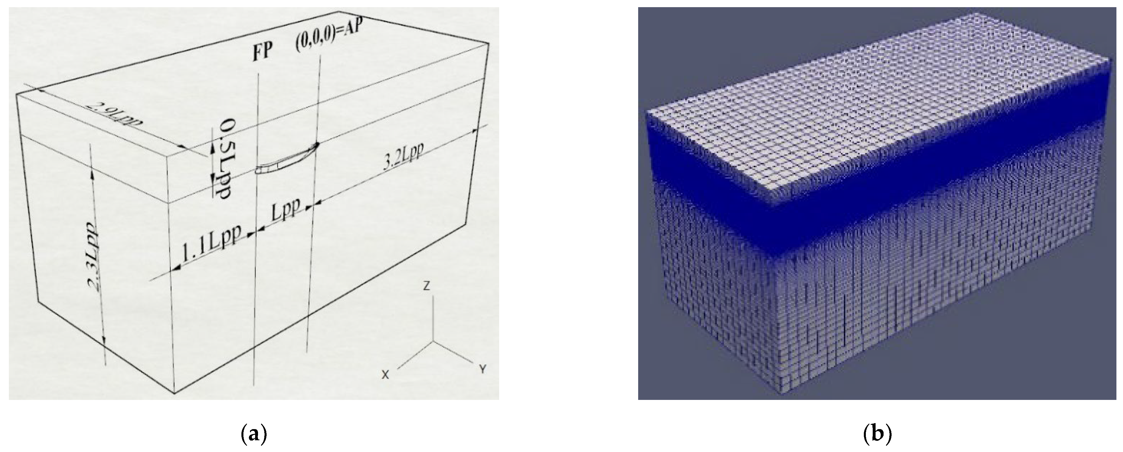
2.4. Domain Size and Grid Topology

For each hull form, coarse, medium and fine grids were built for V & V (Verification and Validation) analysis. The V & V details are in Section 2.6. The refinement ratio $r_G$ between two different grid sizes (spacing) was $\sqrt{2}$ in the x, y and z directions. The ratio $\sqrt{2}$ was applied exactly on the boundaries, so the ratio $\sqrt{8}$ between the total grid numbers was expected. However, due to the unstructured grid method, the total grid number varied depending on element types and their combination. The refinement ratio of the total grid number was maintained as close to $\sqrt{8}$ as possible. As shown in

Table 2. Grid information.

Hull Form	Grid Size	Total Grid Number Ntot.	Layers (Coverage)	Average y+
KLVCC2	Fine	3,572,796	1 (96.9%)	38.8
	Medium	1,180,072	2 (95.2%)	43.1
	Coarse	392,231	3 (97.5%)	77.4
KCS	Fine	1,640,158	3 (96.2%)	99.8
	Medium	572,221	3 (88.3%)	113
	Coarse	208,055	3 (82.1%)	155
JBC	Fine	4,537,454	3 (99.2%)	37.9
	Medium	1,571,444	3 (99.7%)	56.6
	Coarse	590,884	3 (94.5%)	87.3

, the total grid numbers for the coarse, medium and fine grids are 0.39 M (M = million), 1.2 M and 3.6 M, respectively, for KVLCC2. For KCS and JBC, it is 0.21 M, 5.7 M and 1.6 M; and 0.59 M, 1.6 M and 4.5 M. Generally, under the same level of grid density or size, the higher $C_B$ requires more grids to describe the full hull forms with more blunt and curvy geometry. For instance, compare the N_tot. among the fine grids of the three ships. More grid information details are listed in Table 1 and will be explained subsequently.

The KVLCC2 fine grid is the main example used to explain the grid generation method here. The KCS and JBC grid systems were constructed in a similar way, but are slightly different in computation domain size and parameter setup in the built-in grid generator in OpenFOAM v6.0 since their ship lengths, i.e., characteristic length, were different.

The computational domain size is shown in Figure 1a. The origin (0, 0, 0) was located at ship AP (aft perpendicular) with ship baseline along z = 0 and ship length pointing upstream. Thus, ship FP (forward perpendicular) was at (L = L_PP, 0, t), and the undisturbed free surface was initially along z = t, i.e., water height is the ship draft. Because of symmetric flow, only half of the domain corresponding to the starboard side of the flow field was simulated in the -y direction for the three ship hulls. The domain length of the upstream, downstream, bottom, top and side was 1.1L, 3.2L, 2.3L, 0.5L and 2.9L, respectively.

Figure 1b displays the far-field grid distribution. The grid on the boundaries was distributed finer vertically (z direction) near the free surface and around the ship hull. In the x and y directions, the grid has constant spacing distribution. As illustrated in Figure 2, several anisotropic refinement boxes cover the whole ship one by one, from the far to near field. Cartesian grids were constructed level by level around the hull. Inside those refinement boxes, the grid was refined in the x and y directions. For the three hull forms, the grid topology was similar, with a slightly different refinement box setup based on model length and speed. Figure 3 demonstrates the unstructured grid construction and distribution near the ship bow and stern. The grid element was mainly hexahedra, with others like prism, wedge, tetrahedral and polyhedral. The grid across the hull surface was trimmed with the inside portion removed, and then the body-fitted grid was attached to the hull surface as closely as possible. In addition, around the KVLCC2 stern, a local isotropic refinement box was added to capture the curvature geometry in detail, as illustrated in Figure 3a. In this refinement box, the grid was refined in the x, y and z directions. The surface grid on the KCS rudder was two levels finer than the hull surface grid, to describe the much smaller appendage on the relatively large hull body (see Figure 3c).

Finally, to resolve the boundary layer, several layers of layer grid were projected and inserted outward from the surface grid resulting from the previous process. The surface-layered grid generation result is listed in Table 1. KCS and JBC both had 3 layers. The layer number of KVLCC2 was 1, 2 and 3 for the coarse, medium and fine grid, respectively. The layer coverage was near to or over 95%, except for the KCS medium and coarse grids (for which it is lower than 90% due to the low total grid number). For the JBC medium and fine grid, the coverage achieved almost 100%. Some difficulty occurred with the grid layers covering some sharp edges, especially for the slimmer KCS, e.g., its bow leading edge above the bulbous bow in Figure 3e, and the stern trailing edge above the tube shaft tube in Figure 3f. The layer coverage of the KCS fine grid is still as high as 96%.

2.5. Boundary Conditions

The boundary conditions specified in the presented work are explained in

Table 3. Boundary conditions.

	U = (u, v, w)	p	${\mathit{\mu }}_{\mathit{t}}$	$\mathit{k}$	ω	α
Solid surface	(0, 0, 0)	$\nabla p=0$	(11)	(12)	(13)	$\nabla \alpha =0$
Inlet	(−U, 0, 0)	$\nabla p=\rho \mathbf{U}$	$5\times {10}^{-7}$	0.00015	2	$z=t$ for $\alpha =0.5$
Outlet	$\nabla \mathbf{U}=0$ adjusted by α, U0	$\nabla p=0$	$\nabla {\mu }_t=0$	$\nabla k=0$ or 0.00015 for −flux	$\nabla \omega =0$ or 2 for −flux	If α > 1, α = 1 If 0 < α < 1, $\nabla \alpha =0$ If α < 0, α = 0
Top	$\nabla \mathbf{U}=0$ $\mathrm{or} {\nabla }_n\mathbf{U}=0$ for −flux	$p_0$ = 0 or $p_0-0.5{\mathbf{U}}^2$ for −flux	$\nabla {\mu }_t=0$	Same as outlet
Bottom, Mid-plane	Symmetric condition: $\mathbf{n}·\nabla =0$

. The vector U = (u,v,w) is flow velocity. The uniform inflow u on the upstream boundary was set as the negative ship speed, i.e., −U, since the ship length points toward the +x direction. The other variables were constant as well, including turbulence viscosity ${\mu }_t=5\times {10}^{-7}$, turbulence kinetic energy k = 0.00015, specific turbulence dissipation rate ω = 2 and total pressure $p_0$ = 0. Those constants were evaluated with the external flow freestream using common values. In VOF, the volume fraction α = 0.5 was treated as the free surface. The symmetric condition was used on the mid-plane y = 0, bottom and top boundaries, and was mathematically equivalent to the zero-gradient condition in the normal direction. The gradient condition was applied for the static pressure p and α on the hull surface, outlet boundary p and top boundary ${\mu }_t$. Several options for a modified zero-gradient condition are provided in OpenFOAM. A zero-gradient coupled with a reverse flow treatment, called inletOutlet, was utilized for k and ω on the outlet and top boundary, and on the top boundary α. If a positive flux occurs, it is the original zero-gradient; and if a negative flux is detected, the inlet values are forced. For the fixedFluxPressure condition, the inlet p was calculated based on the inlet flux. On the top boundary, the flow velocity was balanced with zero total pressure. It was equipped with the previously mentioned reverse flow treatment as well, named pressureInletOutletVelocity. The imposition of a velocity boundary condition called outletPhaseMeanVelocity on the outlet ensured mass conservation among fluid phases. Accordingly, the free surface height was maintained in the far field. It is also a kind of zero-gradient condition, but the fluid velocity was automatically adjusted based on the average velocity of the mass flux of the two phases. Also, in order to retain the water height on the outlet, the boundary condition variableHeightFlowRate declared zero-gradient α and limited the solved α between 0 and 1.

The no-slip boundary condition, i.e., zero velocity, was imposed with the wall functions for ${\mu }_t$, k and ω as below

$${\mu }_t=\mu \left[{\displaystyle \frac{0.41y^{+}}{\ln \left(9.8y^{+}\right)}}-1\right],$$

(11)

$$\nabla k=0,$$

(12)

$$\omega =\sqrt{{\left[{\displaystyle \frac{6}{0.075{\left(y^{+}\right)}^2}}\right]}^2+{\left[{\displaystyle \frac{k^{+}}{0.41y^{+}}}\right]}^2}.$$

(13)

wherein $y^{+}$ is the non-dimensional normal distance between the wall and control point of the first grid next to the wall. $k^{+}$ is the non-dimensional turbulence kinetic energy. Using a wall function would help with solving the flow field near the wall without using a very fine grid near the solid surface. Thus, computational time consumption and grid number can be reduced. In conjunction with the layer grid built in the previous Section 2.4 and the wall function applied here, the average y+ is of concern and is presented in Table 3. From the fine, to the medium to the coarse grid, the average y+ = from 38 to 87 for KVLCC2 and JBC, and >99 for KCS. All grids are in the logarithmic sublayer of the boundary layer.

2.6. LCGM Correction

The purpose of the procedure is to determine the location of LCG (Longitudinal Center of Gravity, i.e., in the x direction) and ship mass for a ship advancing forward and free to move vertically in a CFD simulation. LCGM stands for LCG-Mass. The surface discretization of a ship model, i.e., the grid generation on the hull surface, would result in the shape used in CFD to deviate slightly from the actual geometry. It is the error between the CFD model and the original ship model. This error not only causes the slight difference in ship mass but also shifts the ship model’s center of rotation a little bit. Without LCGM correction, at the beginning of the simulation the CFD ship model would not be in equilibrium, i.e., it would have initial vertical rotation and translation. With the correction, when the simulation starts, balance is ensured for the gravity and buoyancy at the identical point in the x direction on the ship’s satisfying zero-pitch moment.

On the other hand, between the CFD environment and reality there are certain numerical and modeling errors which should be considered to find proper ship mass and XCG in CFD. In VOF, the free surface is an α distribution across the surface grids around the hull water line. The ship mass is related to the water density solved with α. The gravity effect is calculated in the source term of RANS. It is solved in every grid under all kinds of influence from different grid quality such as aspect ratio, skewness, orthogonality, etc.

In fact, this LCGM correction procedure is equivalent to the ballast weight arrangement in the preparation work of a towing tank test. It is a procedure to align the free surface with the hull waterline by moving around the weight inside the ship model before running the experiment. However, this function does not exist in OpenFOAM. Therefore, the LCGM correction is proposed and implemented to accomplish this task. The procedure is explained as follows, in this example, for a 5.517 m long KVLCC2 ship model:

Initial guess.

First, give a guess value, e.g., LCG or XCG = 3 m, or start with the CG location of the towing tank ship model.

2.

Zero-speed simulation.

Perform the CFD simulation for zero ship speed and no body motions, i.e., static mesh. The boundary conditions are applied as described in Table 2, but U₀ = 0. Also, turn off ${\mu }_t$, k and ω solver since no turbulence occurs under zero ship speed. From the converged result and post-processing, the total pitch moment M_y on the ship model can be obtained, e.g., M_y = 461.3597.

3.

Mass correction.

Correct ship mass with $m=F_Z/g$. Thus, m = 7791.039/9.81 = 794.1936 kg (the actual mass of the ship model is 800.15 kg).

4.

Compensating the couple to achieve a zero-pitch moment.

To carry out the total pitch moment ∑M_y = 0 on the ship model, the compensating couple is m·L = −M_y, e.g., 794.1936 L = −461.3597. It means the LCG or XCG should be shifted to the location with the distance L = −0.580916 m in the x direction.

5.

Update LCG or XCG.

Following the same example, the corrected location of the center of gravity can be obtained: XCG_new = XCG + L = 3 − 0.580916 = 2.419084 m. For the comparison, XCG of the real ship model is 2.9506 m.

6.

Iteration until zero-pitch moment.

Use XCG_new to perform a zero-speed simulation again, and check if M_y = 0. In case of M_y ≠ 0, repeat the above steps 2 to 6 and iterate until M_y = 0 (or stop if a given tolerance is satisfied).

2.7. Verification and Validation (V & V)

The theory of V & V (Verification and Validation) analysis in the presented work follows the ITTC (The International Towing Tank Conference) 7.5-03-01-01 guideline [23]. The verification is to evaluate numerical uncertainty and a confidence range of numerical solutions. This section only focuses on grid uncertainty, i.e., a grid dependence study or grid independence, since our problem is in the steady state. To assess grid uncertainty, the first step is a grid convergence study. Three grids are constructed using systematically refined grid-spacing ${\mathsf{\Delta }x}_i$ (i = 1–3) with the same refinement ratio $r_G$. The subscripts 1, 2 and 3 of the symbols in the following equations represent the three grids: fine, medium and coarse grid, respectively.

$$r_G={\displaystyle \frac{\mathsf{\Delta }{x}_2}{\mathsf{\Delta }{x}_1}}={\displaystyle \frac{\mathsf{\Delta }{x}_3}{\mathsf{\Delta }{x}_2}}=\sqrt{2},$$

(14)

Next, check the convergence using the ratio $R_G$ of the difference between the numerical solutions S_i, which are obtained via the simulations carried out with the three different grid sizes (i = 1, 2, 3 for fine, medium and coarse grid, respectively):

$$R_G={\displaystyle \frac{{\epsilon }_{21}}{{\epsilon }_{32}}}={\displaystyle \frac{s_2-s_1}{s_3-s_2}},$$

(15)

If $0<R_G<1$: monotonic convergence;

If $-1<R_G<0$: oscillatory convergence;

If $R_G>1$, monotonic divergence;

If $R_G<-1$: oscillatory divergence.

In this paper, the ship total resistance coefficient C_T is chosen as S_i.

According to the ratio P between the numerical accuracy rate $P_G$ and the theoretical accuracy order $p_{th}$, the distance metric ${\delta }_{RE}$ from the asymptotic solution can be defined and quantified:

$$P_G={\displaystyle \frac{-\mathrm{l}\mathrm{n} R_G}{\mathrm{l}\mathrm{n} r_G }},$$

(16)

$$P={\displaystyle \frac{P_G}{p_{th}}},$$

(17)

$${\delta }_{RE}={\displaystyle \frac{{\epsilon }_{21}}{{r_G}^{P_G} -1}}.$$

(18)

In this work, the numerical schemes in OpenFOAM are mainly second-order, so set Pth = 2.

If monotonic convergence is achieved, the grid uncertainty $U_G$ is estimated via the factor of safety method with correction factor CF

$$U_G=\left\{\begin{array}{c} FS\left|{\delta }_{RE}\right| , P\le 1 \\ FS·CF\left|{\delta }_{RE}\right|, P>1 \end{array}\right.,$$

(19)

$$CF={\displaystyle \frac{{r_G}^{P_G}-1}{{r_G}^{P_{th}}-1}},$$

(20)

where FS = 1.25 is the factor of safety suggested by ITTC 7.5-03-01-01.

If oscillatory convergence is achieved, the grid uncertainty $U_G$ is evaluated directly using minimal and maximal values of S₁ among the data, as below:

$$U_G={\displaystyle \frac{1}{2}}|\max \left(S_1\right)-\min \left(S_1\right)|.$$

(21)

Considering grid uncertainty $U_G$ and experimental uncertainty $U_D$, the validation uncertainty $U_V$ is

$$U_V=\sqrt{U_G^2+U_D^2}.$$

(22)

Finally, the error E is defined by the difference in percentage between experimental data D and simulation value S_i:

$$E=\left(D-S_i\right)\%D.$$

(23)

By comparing E for i = 1 to $U_V$, if $\left|E\right|\le U_V$, the CFD method is validated at the $U_V$ range.

3. Results

3.1. V & V for Static Mesh

First, neglecting the ship vertical motion, i.e., the fixed ship attitude, the CFD resistance test was simulated using static mesh. The three hull forms were all in the even-keel condition. To perform V & V analysis and estimate uncertainty, a simulation of the fine, medium and coarse grids was required. The results of the total resistance coefficient C_T, the error and the V & V analysis are listed in

Table 4. Total resistance coefficient and V & V result for KVLCC2 (static mesh, Re = 5.741 × 10⁷, Fr = 0.142).

Parameters		D	S1	S2	S3	rG	RG	ε12%S1	pG/pG,th	UG%S1	UD%D	Uv%
CT × 103	Value	4.568	4.614	4.814	5.219	1.414	0.493	−4.335	1.020	4.45	1.0	5.56
	E%D		−1.01	−5.39	−14.3		Verified					Validated

,

Table 5. Total resistance coefficient and V & V result for KCS (static mesh, Re = 1.46 × 10⁷, Fr = 0.26).

Parameters		D	S1	S2	S3	rG	RG	ε12%S1	pG/pG,th	UG%S1	UD%D	Uv%
CT × 103	Value	3.711	3.527	3.555	3.755	1.414	0.142	0.807	2.813	0.96	1.0	1.39
	E%D		4.97	4.20	−1.19		Verified					--

and

Table 6. Total resistance coefficient and V & V result for JBC (static mesh, Re = 7.46 × 10⁷, Fr = 0.26).

Parameters		D	S1	S2	S3	rG	RG	ε12%S1	pG/pG,th	UG%S1	UD%D	Uv%
CT × 103	Value	4.289	4.400	4.577	5.961	1.414	0.128	4.023	2.967	5.03	1.0	5.26
	E%D		−2.59	−6.72	−39.0		Verified					Validated

for each ship model, respectively. The C_T values predicted with CFD for fine, medium and coarse grid are S₁, S₂ and S₃, respectively. The experimental C_T value is D. The error E%D is defined as (23). As the grid number increases, the over-predicted KCS C_T becomes under-predicted. Instead, for the full hull form (KVLCC2 and JBC), the C_T values are all over-predicted. For the three hull forms, error reduces as the grid becomes denser. Up to fine grid, C_T error lowers to 1% for KVLCC2, reaches 2.6% for JBC, and is less than 5% for KCS. For coarse grid, only the KCS C_T error is acceptable, at about 1%. For both KVLCC2 and JBC, the errors are larger than 10%. For medium and fine grid, the average error is 4% with a minimum of 1%, and all are below 7%.

The results of the three hulls satisfy the 0 < R_G < 1 condition, meaning that the difference between the fine and medium grid results is smaller than that between the medium and coarse grid results, i.e., monotonic convergence is achieved. In the tables, r_G = 1.414 is the refinement ratio $\sqrt{2}$ mentioned in Section 2.7 In other words, the CFD method and our simulation results have been verified, and grid independence is confirmed. For uncertainty estimation, it is found that the total uncertainties of KVLCC2 and JBC are around 5% larger than the error of S₁. In conclusion, the CFD method here for both ships is validated. Although the KSC uncertainty is merely 1.4%, S₁ has a slightly larger error, and then U_v is smaller than the E%D of S₁. It represents the fact that the convergence and comparison among the CFD results themselves are more confident than CFD compared with the experimental results. Therefore, the KCS result does not qualify for validation. In Section 3.3, this issue will be resolved with the improved E%D of S₁, using the XCGM correction. In addition, the experimental uncertainty U_D = 1% for every ship was taken from the towing tank tests at the G2010 and T2015 conferences.

3.2. LCGM Correction

To perform the LCGM correction procedure, the fine grids of KVLCC2 and KCS were selected. For JBC, the medium grid was chosen to save computational time.

Table 7. LCGM correction results for three hull forms.

	KVLCC2 (Fine Grid)		KCS (Fine Grid)		JBC (Medium Grid)
	Experimental Values	Corrected Values	Experimental Values	Corrected Values	Experimental Values	Corrected Values
Mass (kg)	1600.311	1586.416	1648.150	1650.811	2782.013	2779.125
XCG (m)	2.9506	2.9411	3.5316	3.5283	3.67833	3.67796
YCG (m)	0		0		0
ZCG (m)	0.31969		0.4359		0.3323
$I_x$ (kg$·$m2)	256.046	253.823	273.822	274.264	563.358	562.773
$I_y$ (kg$·$m2)	3044.54	3018.107	5457.232	5466.042	8519.915	8511.070
$I_z$ (kg$·$m2)	3044.54	3018.107	5457.232	5466.042	8519.915	8511.070

presents the LCGM correction results for the three ship models. The origin was at (0, 0, 0). As seen in the table, two parameters were mainly corrected: ship mass and LCG (Longitudinal Center of Gravity in the x direction, i.e., XCG). The corrections are all small changes but are more significant for KVLCC2 among the three hulls; its mass decreased 0.87% from the model mass in the experiment. XCG shifted 0.32% toward the ship stern. For KCS, the mass rose 0.16%, but it was reduced by 0.1% for JBC, and both ships’ XCG moved 0.1% toward their sterns.

Consequently, mass correction would influence moments of inertia of mass. However, in a ship resistance test, a steady state would eventually be achieved. It means the motion displacement would not change with time, i.e., there is no acceleration. Although different moments of inertia may only affect the motion and flow field during the transient period, in this study, the moment of inertia is still adjusted correspondingly, as indicated in Table 6. The uniform distribution of the ship model mass is assumed in the CFD simulation to be like that of the real model in the towing tank experiment. The moment of inertia of mass is:

$$I=m{K}^2,$$

(24)

In the above Equation (24), m is the ship mass and K is the radius of gyration about a given axis. The non-dimensional k was suggested by the conference website SIMMAN2014 [24] for KVLCC2 and T2015 [22] for KCS and JBC for the x, y and z axis, respectively:

$$K_{xx}/B=0.4,$$

(25)

$$K_{yy}/L_{pp}=K_{zz}/L_{pp}=0.25.$$

(26)

The next section will conclude that the mass correction mainly affects the sinkage and the XCG influences the trim angle. The mass change means the ship volume displacement changes and then the ship draft changes. The XCG difference causes buoyancy and causes gravity to act at a different point. Since the center of gravity deviates from the original balanced position, the extra moment is generated to rotate the ship body to reach another equilibrium. The rotation causes the trim angle.

3.3. Resistance Test for Dynamic Mesh

This section will discuss the result of the CFD resistance test using dynamic mesh, i.e., the flow and motion solver were coupled in the simulation. Thus, C_T, sinkage σ/L and trim τ were predicted together via CFD. The detailed results with and without LCGM correction are listed in

Table 8. Total resistance coefficient and V & V result for KVLCC2 (dynamic mesh, Re = 5.741 × 10⁷, Fr = 0.142).

CT × 103		S1	S2	S3	rG	RG	ε12%S1	pG/pG,th	UG%S1	UD%D	Uv%
Without correction	Value	4.808	5.204	5.272	1.414	5.873
	E%D	−5.26	−13.93	−15.40		-
LCGM correction	Value	4.677	4.981	5.493	1.414	0.593	−6.497	0.753	9.48	1.0	12.18
	E%D	−2.38	−9.02	−20.24		Verified					Validated

,

Table 9. KVLCC2 sinkage and trim result (dynamic mesh).

Case	Type	Sinkage		Trim
		100σ/L	E%D	τ°	E%D
Experimental values (D)		−0.116		−0.13
Fine grid (S1)	Without correction	−0.153	−32.0	−0.230	−76.6
	LCGM correction	−0.094	18.6	−0.127	2.49
Medium grid (S2)	Without correction	−0.104	10.5	−0.337	−159
	LCGM correction	−0.095	18.2	−0.1296	0.26
Coarse grid (S3)	Without correction	−0.169	−45.8	−0.233	−79
	LCGM correction	−0.11	4.99	−0.131	−0.86

,

Table 10. Total resistance coefficient and V & V result for KCS (dynamic mesh with LCGM correction, Re = 1.26 × 10⁷, Fr = 0.260).

CT × 103	S1	S2	S3	rG	RG	ε12%S1	UG%S1	UD%D	Uv%
Value	3.697	3.691	4.056	1.414	−0.019	−0.18	4.93	1.0	5.03
E%D	0.36	0.55	−9.30		Verified				Validated

,

Table 11. KCS total resistance, sinkage and trim prediction (Re = 1.26 × 10⁷, Fr = 0.260).

Parameters		EFD (D)	S1 (Without Correction)	S1	S2	S3
				(LCGM Correction *)
CT × 103	Value	3.711	3.69383	3.69748	3.691	4.056
	E%D		0.46%	0.36%	0.55%	−9.30%
σ × 102 (m)	Value	−1.394	−1.364	−1.40694	−1.40688	−1.343
	E%D		2.14%	−0.93%	−0.92%	3.64%
τ°	Value	−0.169	−0.16617	−0.16876	−0.166	−0.153
	E%D		1.68%	0.14%	1.63%	9.55%

* Only correct the mass since the trim is well-predicted.

and

Table 12. Total resistance coefficient and V & V result for JBC (dynamic mesh with LCGM correction, Re = 7.46 × 10⁷, Fr = 0.142).

CT × 103	S1	S2	S3	rG	RG	ε12%S1	pG/pG,th	UG%S1	UD%D	Uv%
Value	4.505	4.712	4.974	1.414	0.79	4.59	0.340	21.62	1.0	22.73
E%D	−5.04	−9.86	−15.97		Verified					Validated

. The same grid set of the coarse–medium–fine grid is adopted for the static and dynamic mesh. In fact, the dynamic mesh simulation could be started from the static mesh result as the initial solution. In other words, the static mesh simulation could be restarted with the dynamic mesh and motion solver turned on.

For KVLCC2 C_T, the V & V analysis is also conducted. Table 8 indicates that, without the ship mass and center of gravity corrected with the LCGM correction, the monotonic convergence cannot be accomplished. Although both errors |E%D| decrease as the grid number increases, only through using LCGM correction is our dynamic mesh result verified and grid-independent. Furthermore, the higher uncertainty for the dynamic mesh reflects on the fact that the grid is deformed, i.e., the grid deformation causes higher numerical uncertainty. The uncertainty of the static mesh (Table 4) is around 5%. With the correction, the dynamic mesh reports more than 10% uncertainty, but the results are still validated since U_v is larger than the S₁ error, or S₁ is close enough to the experimental data. Except for the coarse grid, the correction reduces the C_T errors, e.g., the |E%D| without and with the correction is from 5% down to below 3% for the fine grid. For the medium grid, the deviation is expected, since the correction is based on the fine grid, and so the |E%D| is only reduced from nearly 14% to 9%. Since the coarse grid essentially can just not describe the geometry well, the resultant mass and XCG are not suitable for the coarse grid geometry.

KVLCC2’s σ/L and τ results are shown in Table 9. Without the correction for ship mass and XCG, except for the medium grid which under-predicts 10% for sinkage, the others over-predict dramatically. The trim error of the medium grid reaches even 159% and is close to 80% for the coarse and fine grids. The sinkage error is over 30% for the coarse and fine grids. After the ship mass and XCG are updated using the LCGM correction, the results of ship vertical motion prediction are improved significantly. In particular, the trim |E%D| drops from nearly or over 80% to below 3%, and is even less than 1% for the medium and fine grids. By comparison, the sinkage is not as close to the experimental data as the trim, but the error decrease is still evident for the fine and coarse grids. The ship vertical motions and resistance are correlated in the following explanation for KVLCC2. Without the LCGM correction, for all grids, their bows down are very large. For the fine and coarse grids, the ship and bow sink too much but, for the medium grid, the ship does not sink enough. In the static mesh result (Table 4), the ship resistances are already over-predicted. Thus, all three ship resistances increase to become more over-predicted. The lighter ship mass and more backward XCG position provided by the correction reduces all the resistance and motion |E%D| from the results without the correction. The correction causes the ship and bow to sink less, and the |E%D| of the motions tends to become smaller as the grid number decreases. Sinkage |E%D| is from around 18% for the fine and medium grids to 5% for the coarse grid. Trim |E%D| is from around 2.5% for the fine grid to less than 1% for the medium and coarse grid. In contrast, the resistance |E%D| decreases as the grid number increases (Table 4 and Table 8). The E%D of (S₃, S₂, S₁) = (−14.3%, −5.39%, −1.01%) for the static grid. Error (S₃, S₂, S₁) = (−16%, −9.72%, −5.23%) without the correction. Error (S₃, S₂, S₁) = (−17.7%, −9.02%, −2.71%) with the correction. High grid density and a well-described surface are the important aspects to predict calm-water resistance instead of ship vertical motion.

For KCS, the V & V results for C_T predicted using the dynamic mesh and LCGM correction are provided in Table 10. The comparisons with and without LCGM correction for C_T, σ/L, and τ are in Table 11. Without the correction, only the fine grid was tested, because the trim |E%D| without correction is fairly small, i.e., less than 2% (S₁ for τ labeled under no correction in Table 11), and the correction only produces a 0.1% difference for XCG (Table 7). Thus, only ship mass was corrected with the LCGM correction procedure. The XCG was maintained as the original ship model setup in the experiment. With the correction, the |E%D| of C_T is clearly improved for all grids because all C_T is increased by the ship’s vertical motions and becomes closer to D = 3.711 (Table 5). For S₁ in Table 5 and Table 10, the under-predicted C_T error is reduced to less than 1% from approximately 5%. As a result, the KCS result with the correction is validated with oscillating convergence. In Table 11, without the correction, the motion error is around 2%. As the ship mass is adjusted to be more suited to the CFD environment, σ and τ |E%D| further decline, below 1% (S₁ in Table 11). Due to the slightly heavier corrected ship mass, the ship and bow sink more, i.e., larger |σ| and |τ|. It is true for σ and τ of S₁, and σ of S₂ compared with S₁ with no correction, but not for the other values, because the correction is based on the fine grid, and the coarser grid loses more geometric fidelity. S₂ with the correction provides similar results to S₁ without the correction for C_T~3.69 and |τ|~0.166, but |σ| is nearly the same as S₁ with the correction (~1.4069). Also, as the grid number increases with the correction, all |E%D|s of C_T, σ and τ are basically reduced (considering σ of S₁ and S₂ is nearly the same as −1.4069). For the coarse grid, C_T using the correction, σ and τ results all become worse. For the slim and fast hull forms, the grid number is not required to be too high for the acceptable resistance prediction. The dynamic mesh might worsen the results if the grid is too coarse. If the grid number and ship mass are correct, the resistance and motion prediction will be further improved.

For JBC, the V & V result of the dynamic mesh simulation with the LCGM correction can be found in Table 12. The results for C_T, σ/L and τ are in

Table 13. JBC total resistance, sinkage and trim prediction (Re = 1.26 × 10⁷, Fr = 0.260).

Parameters		D	S1 †††	S2 (Without Correction)	S2 †††	S3 †††
CT ×103	Value	4.289	4.505	4.719	4.712	4.974
	E%D		−5.04%	−10.03%	−9.86%	−15.97%
† CF ×103	Value	3.159	3.093	3.111	3.108	3.087
	E%D		2.08%	1.51%	1.62%	2.26%
†† CP ×103	Value	1.130	1.412	1.608	1.6048	1.886
	E%D		−24.92%	−42.29%	−41.99%	−66.88%
σ [%LPP]	Value	−0.086	−0.0855	−0.0912	−0.0853	−0.0781
	E%D		0.56%	−6.10%	0.78%	9.19%
τ [%LPP]	Value	−0.180	−0.188	−0.197	−0.1908	−0.176
	E%D		−4.33%	−9.60%	−5.97%	2.38%

^† ITTC 1975 formula. ^†† C_P = C_T − C_F. ^††† with LCGM correction (from Table 11).

. Without the correction, only the medium grid was tested. Like KVLCC2, all C_T is already over-predicted in the static mesh results (Table 6). With the correction, the motions cause larger C_T and become more over-predicted for S₁ and S₂. Although the C_T of S₃ decreases, it is still greatly over-predicted. The uncertainty increases to around 23%, but the increased |E%D| of S₁ is still small enough, i.e., 5% is considered a good prediction for ship resistance. Overall, monotonic convergence, Verification and Validation all remain. For S₂, C_T error is over-predicted at 7% (Table 6). Without correction, it rises to 10% over-prediction due to the motions. With the LCGM correction, it drops to slightly less than 10%. It is mainly because the sinkage is significantly improved from the over-predicted 6.1% to the under-predicted 0.78%. The improvement in the over-predicted trim error is relatively minor (from around 10% to 6%). Although the LCGM correction is based on the medium grid, it helps the fine and medium grid simulations. Errors |E%D| of σ and τ for S₁ are smaller than the S₂ results, and the τ of S₃ is only under-predicted at around 2%, which is the best |E%D| overall.

The resistance component for JBC is further analyzed in Table 13. In the resistance decomposition for the experimental data, the friction resistance coefficient C_F is estimated using the ITTC 1975 formula, and the pressure coefficient C_P is the difference between C_T and C_F. The main source of resistance error is from C_P. The over-predicted C_P error reaches up to 25% for S₁, 42% for S₂ and 67% for S₃, but C_F error is around 2% for all. It concludes that, in CFD ship resistance prediction, the friction component is very close to the flat plate assumption, and the pressure component can be improved by increasing grid density.

3.4. Flow Field Analysis

3.4.1. Ship-Making Wave Pattern

For the free surface elevations around KVLCC2, Figure 4 shows the CFD results for the presented work using the static and dynamic grids, respectively. For KCS, Figure 5 illustrates the free surface elevation solved with the CFD static grid. For JBC, Figure 6 depicts the CFD free surface elevation (static grid). In the figures, the wave amplitude z is non-dimensionalized by the ship length L. In Figure 4, Figure 5 and Figure 6, the results of the coarse, medium and fine grids are in order, from the top to bottom. The experimental data compared in this section, corresponding to KVLCC2, KCS and JBC, respectively, are presented in Figure 9 from [1], Figure 7 from [1], and Figure 1.3a-5 from [9,22].

For KVLCC2 and KCS, the experimental measurement clearly shows the ship-making wave pattern, i.e., the Kelvin wave system, including diverging and transverse waves. For KVCC2 and JBC, because of the low ship speed (Fr = 0.142), the wavelength and amplitude are short (around 0.13 ship length). However, the wave pattern of JBC is more scattered. Instead, due to the high ship speed (Fr = 0.26), long wavelength and large amplitude (around 0.42 ship length) are observed for KCS. Basically, CFD simulation can resolve the wave pattern effectively if the grid is fine enough. For the main concern of this study, the ship resistance prediction, the grid distribution is designed to be denser around the hull body, as seen in Figure 2a. The bow and front shoulder wave crest and the stern wave trough are resolved well for all ships and different grid sizes.

Although the grid is also refined near the free surface in the vertical direction, i.e., the z direction in Figure 2a, the grid density decreases gradually in the x and y directions to reduce computational consumption, as shown in Figure 2b. As a result, the far field wave propagation apparently decays. In other words, the wave pattern in the far field is not clear. For instance, in Figure 4a, the diverging waves of KVLCC2 are clear around the hull body within 1~2 ship beams for coarse, medium and fine grid. Outside 1~2 ship beams, only the fine grid results can resolve the diverging and transverse waves in the far field and downstream (see the black arrows at the bottom of Figure 4a). A comparison between Figure 4a,b shows that the dynamic grid, i.e., the grid deformation, barely influences the free surface wave pattern solution. Although the sinkage and trim prediction are improved with the LCGM correction, as mentioned in Section 3.3, the ship draft change and ship motions are too small to have an impact on the main features of the wave pattern. In Figure 4, the square-shaped disturbances with very small wave amplitudes occur around the region of grid refinement level change, except for at the bottom of Figure 4a. They are contoured green, representing z/L~0. In the static grid, it is related to the interpolation error for the free surface inside the large grids of the far field. Thus, those disturbances are eliminated in the fine grid. However, they are all evident, and worsen in the dynamic grids, even for the fine grid. The grid deformation cutting through the free surface strengthens those disturbances, especially in the far field grid, where the slight deviation from z = 0 makes the square-shaped disturbances stand out more from the background.

For KCS, the wave pattern is more distinct, with a larger length and amplitude due to high Fr. The wave amplitude also increases as grid density increases. As pointed out by the arrows in Figure 5c, the highest z/L of the wave crest becomes higher, and the lowest z/L of the wave trough becomes lower from the coarse, medium to fine grid. The wave pattern, i.e., the contour profile, of the fine grid results agrees with the experimental results very well, as indicated in Figure 5c. The dense distribution contour lines of the stern wave crest can be observed in both CFD and the experiment, which is caused by the KCS flat transom. The high stern waves were also revealed by Kim et al. [1] and Jasak et al. [2], and do not emerge from behind the KVLCC2 and JBC stern.

JBC and KVLCC2 are full hull forms, and JBC is even blunter, i.e., a higher CB (Table 1). Thus, the clearer and lower stern shoulder appears in all JBC CFD results. The CFD grid is not fine enough to capture the scatter wave pattern of JBC in the downstream far field. Only the diverging waves are well-resolved around the hull, with increasing wave amplitude as grid density increases (refer to the pointed arrows in Figure 6c).

3.4.2. Boundary Layer and Wake Profile

The velocity field distribution on the propeller plane, i.e., the nominal wake velocity profile, is analyzed in this section. For both KVLCC2 and KCS, the propeller plane is on the x/L = 0.9825 plane, and x/L = 0.985714 for JBC. The velocities (u, v, w) in the x, y, z direction are all non-dimensionalized by model ship speed U. Axial velocity u/U is plotted with contour lines or color flood contour, and cross flow is illustrated with vector field (v/U, w/U) in the figures. In addition, the x/L = 0.85 plane is plotted using the same format to investigate the upstream boundary layer before the propeller plane.

For KVLCC2, Figure 7 shows the CFDs result for the static and dynamic grids, including the different grid sizes. The x/L = 0.85 plane results are also presented in Figure 8 for the CFD static and dynamic grid. The observation of the x/L = 0.85 plane is to understand the boundary layer development along the ship stern wall before the propeller plane. For KCS and JBC, Figure 9 only presents the static grid results. The results of the coarse, medium and fine grids are shown in Figure 7, Figure 8 and Figure 9, in the order from the top to bottom.

Basically, the CFD can capture the flow field features of the nominal wake and agree with the experimental result, especially as the grid number increases. These features include the bilge vortex aside from the propeller center, the secondary vortex beneath the propeller center, and the upward flow in the far field. The bilge vortex is generated upstream, at the joint between the ship bottom and side wall, and sheds downstream where the ship’s stern shape sharpens (streamlines) vertically and laterally. It rotates from the ship bottom to the side wall, and finally flows into the propeller plane. The bilge vortex is normally located around the intermediate layer of the boundary layer. The secondary vortex is induced by the bilge vortex, so it rotates in the opposite direction. Also, it is accompanied by the low-speed area, i.e., the inner boundary layer developed from the ship bottom upstream. The upward flow corresponds to the outer boundary layer with high flow velocity. Its direction tends to point toward the ship centerline because of the three-dimensional sharpening stern shape, as mentioned previously, and the rotational direction of the bilge vortex. For KVLCC2 and JBC, due to the blunt stern and full hull form, those features are distinct. For KCS, the hull form is much slimmer, and the ship speed is higher, so that only the bilge vortex is more dominated.

For KVLCC2, the CFD results show those features clearly. The vertical position of the bilge vortex is from around z/L = −0.055 to −0.04, corresponding to the hook or U-shaped velocity profile of u/U = 0.4–0.6, i.e., the green contoured area. It coincides with the experiment [1,25] well. The reference experiment here is shown in Figure 3.4, from [25], which originated from [1]. The difference occurs in the bilge vortex width and lateral location. As the grid grows denser, the bilge vortex becomes narrower laterally, and its center moves closer to the centerline. In the experimental result [1,25], the vortex center is around z/L = −0.045 and slightly to the right side of y/L = −0.01. Consequently, the medium grid result concurs with the experiment more, while that of the fine grid is too narrow and is almost close to y/L = −0.005. This implies that the fine grid may resolve new or unknown phenomena which might not exist in the experiment or may not be detected by the current measurement technology.

The secondary vortex appears in all the CFD results for KVLCC2. However, in the coarse grid, the low-speed area u/U < 0.2 only takes place around the solid surface of the propeller shaft tube. This could be obtained once the grid density increases similar to that of the medium and fine grid. In the experiment, the low-speed area is an isolated u/U = 0.2 contour line with a width of around y/L = −0.005. In the medium and fine grid results, the low-speed area u/U < 0.2 connects to the boundary layer around the shaft tube wall, which differs from the experiment. Even so, the size and width are much smaller for the fine grid results, and are considerably close to the experimental results. Refining the grid and dynamic grid would improve the u/U prediction in the outer boundary layer. The upward flow behavior is all preserved well. For instance, by checking the contour line of u/U = 0.9, a large bulge toward the bottom-left corner can be found in the experiment. It is around y/L = 0.055 (corresponding to −0.05 in the CFD portside result) and z/L = −0.035 in the experiment. In the coarse grid, it extends much deeper and wider, e.g., around y/L = −0.07 and z/L = −0.05. As the grid number increases for the fine grid, it shrinks to around y/L = −0.06 and z/L = −0.04, close to the experimental values. The same trend is observed for both the static and dynamic grids. Since larger wake area reflects larger ship resistance, it also explains the trend in Table 4 (static grid) and Table 8 (dynamic grid): the over-predicted error decreases from S₃ and S₂ to S₁. In addition, the u/U = 0.9 contour lines above z/L = −0.01 all long-extend to the left, around or beyond y/L = −0.07, except for the dynamic fine grid close to the experimental y/L, which is around −0.065 (equivalent to 0.0.65 in the starboard field). Also, there is a high-speed area (u/U > 1) in the coarse grid results below z/L = −0.065, which is unrealistic and does not exist in the experimental, medium or fine grid results.

The comparison in Figure 8 indicates that the u/U contour lines are clearly smoother, with denser (v, w) vector distribution as the grid number increases, since the local refinement box does not cover this stern part. The behavior of the outer boundary layer, e.g., u/U = 0.9, on x/L = 0.85 here supports the previous conclusion of x/L = 0.9825. However, the u/U = 1 profile of the finer grid deviates from the experiment. In the experiment (Figure 3.3 in [25], originating from [1]), the u/U = 1 intersects the horizontal axis at y/L = 0.06; however, in the medium and fine static grids, and in the fine dynamic grid, the u/U = 1 keeps extending to the right. In contrast, the intersection in the medium grid is at x/L = 0.08, The results of the static and dynamic grid in the same grid size are nearly the same. The u/U = 1 intersection might be able to be improved slightly through the use of a dynamic grid. For example, for the coarse grid, the intersection is around x/L = 0.075 and 0.067 for the static and dynamic grids, respectively. In the medium grid, there is no intersection for the static grid, but it intersects around x/L = 0.08 for the dynamic grid. However, it does not work for the fine grid. Both static and dynamic grid results show no intersection.

For the bilge vortex behind KCS, the experimental (Figure 10c in [1]) and CFD results for the medium and fine grids, shown in Figure 9a at the middle and bottom, agree with each other well. It is located from around y/L = −0.005 to −0.01 and from z/L = −0.04 to −0.02. As seen at the top of Figure 9a, the grid is so coarse that there is no grid node along y/L = −0.005 (referring to the vectors). Consequently, the coarse grid cannot resolve the bilge vortex. As for KVLCC2 and JBC, the bilge vortex of the medium and fine grid coincides with the u/U = 0.4~0.6 area but does not have the hook or U-shaped velocity profile. The secondary vortex and low-speed area beneath the propeller center are very obscure. The coarse grid is too coarse to resolve them as well. The medium grid only captures the vector direction change at y/L = −0.003 and z/L = −0.03, as seen in the middle of Figure 9a. Only the fine grid can predict the secondary vortex, which is from near y/L = −0.002 to −0.004 and from z/L = −0.036 to −0.032, as shown in Figure 9a, at the bottom, with the low-speed area u/U = 0.3–0.35. Basically, the coarse grid only presents the upward flow. However, the characteristic of the outer flow field is still omitted in Figure 9a (top). The experiment reveals a bulge toward the bottom-left corner along the contour line of u/U = 0.9 around y/L = −0.04 and z/L = −0.02. The coarse grid result only shows a smooth declining curve for u/U = 0.9. The bulge is resolved for the medium and fine grid around y/L = −0.035 and z/L = −0.02. Using the y/L value as a reference for the lateral thickness of the boundary layer, the medium and fine grid results are thinner than the experimental ones. This is the reason S₁ and S₂ are both under-predicted in Table 5. The area of u/U > 0.95 in Figure 9a (top) is obviously smaller than that in Figure 9a (middle and bottom). This implies a thicker boundary layer for the coarse grid. This explains why S₃ is over-predicted and greater than S₁ and S₂ in Table 5. Even with the LCGM correction, S₁ and S₂ are both still under-predicted, and S₃ is much more over-predicted (Table 10). Overall, the flow field patterns, such as bilge vortex and u/U contour lines, are maintained fairly consistently between the medium and the fine grid. The flow field resolution is enhanced by increasing the grid number, which includes smoother contour lines and denser vector distribution, as shown in Figure 9a (middle and bottom).

As illustrated in Figure 9b, the JBC wake field features similar flow patterns to KVLCC2, including the bilge vortex with a U-shaped velocity profile, a secondary vortex with a low-speed area beneath the propeller shaft tube and an outer field upward flow. However, JBC is a much blunter and fuller hull form with higher $C_B$. Thus, the much lower axial velocity appears in the core of the bilge vortex. The reference experiment is shown in Figure 3 from [9] and in Figure 1.3a-2 from [22]. The region divided by red dashed line in the bottom-right of the three figures in Figure 9b corresponds to the measurement zone [9,22]. The core u/U in the experiment reaches below 0.2, but all CFD can only reach u/U = from 0.3 to 0.4, which is still much lower than u/U = from 0.4 to 0.6 for KVLCC2. The coarse grid cannot resolve the core in the U-shaped profile. The medium and fine grid are able to capture the core with u/U = from 0.3 to 0.4, as shown in Figure 9a, at the middle and bottom, respectively. To resolve the u/U < 0.2 core, the grid is required to be much finer. The experiment and the CFD results show the agreement for the bilge vortex location, which is y/L = −0.01 and z/L = from −0.05 to −0.045. For the low-speed area, the medium and fine grid can achieve u/U < 0.2, which is as low as the experiment. The value of the low-speed area is similar between JBC and KVLCC2, i.e., u/U < 0.2, but their u/U < 0.2 profiles are different. The u/U < 0.2 area of JBC is narrower and extends downward. In particular, the fine grid profile is closer to the experimental results. As discussed previously for the different hull forms, the flow field resolution increases through increasing the grid number. A finer grid would predict a flow field closer to the experimental results. The resistance trend (Table 6 and Table 12) also supports this conclusion: the error value decreases from S₃ to S₂ and S₁. However, the JBC fine grid might be also too fine to resolve a new phenomenon or a phenomenon which cannot be measured through the current experiment. In Figure 9a (bottom), around y/L = −0.02 and z/L = −0.05, a sharp and upward-pointing contour line bulge for u/U = 1.0 occurs, but it does not appear in the experimental, coarse or medium grid results.

3.5. Computational Time and Resources

In this section, the computational resources and time consumption used in this work are provided, and are shown in

Table 14. Computational time and resources.

Ship Model	Mesh Type		Execution Time		Total Iterations	Sec per Iteration	Used Processors	CPU	Threads
		Case	Sec	Days
JBC	Static mesh	S1	213,727	2.47	8022	26.64	24	E5-2678v3	24 × 2
		S2	66,137.8	0.77	11,307	5.85	6	i5-8500	6
		S3	84,185	0.97	24,928	3.38	4	i5-8500	6
	Dynamic mesh	S1	684,757	7.93	38,907	17.60	36	E5-2699v4	44 × 2
		S2	399,110	4.62	24,500	16.29	11	E5-2699v4	44 × 2
		S3	329,842	3.82	198,393	1.66	28	E5-2690v4	44 × 2
KCS	Static mesh	S1	50,195.8	0.58	20,000	2.51	12	E5-2678v3	24 × 2
		S2	27,471.3	0.32	40,000	0.69	12	E5-2678v3	24 × 2
		S3	39,268.9	0.45	30,000	1.31	12	E5-2678v3	24 × 2
	Dynamic mesh	S1	174,994	2.03	30,020	5.83	33	2696v3	36 × 2
		S2	64,542.5	0.75	30,000	2.15	24	2696v3	36 × 2
		S3	46,372.2	0.54	30,000	1.55	9	2696v3	36 × 2
KVLCC2	Static mesh	S1	76,136.2	0.88	9460	8.05	12	3950x	32
		S2	27,298	0.32	13,000	2.10	12	3950x	32
		S3	15,373.1	0.18	13,000	1.18	12	3950x	32
	Dynamic mesh	S1	540,493	6.26	38,000	14.22	12	3950x	32
		S2	196,267	2.27	48,541	4.04	12	3950x	32
		S3	57,240.7	0.66	70,256	0.81	12	3950x	32

. Basically, the larger grid number costs more time, and dynamic mesh requires more time than static mesh. There are some exceptions. Use sec per iteration as the comparison standard. For KCS static mesh, S₃ is slower than S₂. For the S₃ of JBC and KVLCC2, the static mesh is slower than the dynamic mesh. This is because the small grid size cases were often executed with the other cases. The JBC static mesh S₂ and S₃ simulations were performed on a virtual machine running on a Windows machine with a single CPU. All KVLCC2 cases were conducted on a single CPU computer. The rest of the cases were finished on the Linux servers with dual Intel Xeon third- or fourth-gen CPUs. Higher grid numbers would occupy more processors but, typically, only half of the cores or fewer were used. The execution time shown in Table 14 is the real time consumed in total to complete those total iterations. However, the case running was normally maintained longer to ensure the iterative convergence, as shown in Figure 10. Thus, the running could be shortened. For JBC S₂ in Figure 10, the total resistance (RT) result is the averaged value of the iteration interval from 45176 to 49984. The value oscillation, i.e., iterative uncertainty U_i, is only 0.0058% of RT. For KCS and KVLCC2 S₁ in Figure 10, the iteration interval is from 26,000 to 30,020 with U_i = 0.24%, and from 28,000 to 38,000 with U_i = 1.28%, respectively. The KVLCC2 iteration is more unstable, with some random peaks because local time stepping was used, and this is a pseudo-transient assumption for steady problem.

4. Discussion

The sinkage and trim prediction in the ship resistance simulation performed with OpenFOAM has been successfully improved via the proposed LCGM correction procedure. The LCGM procedure is an iterative method to find the proper mass and the location of the center of gravity in the x direction (ship longitudinal direction), i.e., XCG for the ship model in the CFD environment. In the LCGM procedure, the static equilibrium for a zero-pitch moment is achieved in the zero-speed CFD simulation. The procedure is required because the object geometry in CFD would not be exactly identical to the actual ship model, since the ship surface is discretized with the computational grids. By increasing grid number, the ship’s geometry in the CFD simulation will be approximately closer to the model in reality but will not be exactly the same. The LCGM procedure is tested successfully in the presented work for three different hull forms, and the results are verified and validated.

For static mesh simulation, i.e., sinkage and trim are neglected, the ship resistance error reaches less than 3% over-prediction for KVLCC2 and JBC as the grid number increases to the finest. Instead, the KCS error rises to around 5% under-prediction. Using the LCGM correction, the ship mass is 0.87%, is 0.1% lower for KVLCC2 and JBC, but increased by 0.16% for KCS. XCGs are shifted forward 0.32% for KVLCC2 (fine grid) and 0.1% for KCS (fine grid) and JBC (medium grid). Those very small correction values would mainly improve the sinkage and trim predictions in dynamic mesh simulations. Basically, ship motions would increase resistance. The resistance error increases for KVLCC2 and JBC but is still small enough to be considered accurate. It is over-predicted to be less than 3% and around 5% for KVLCC2 and JBC fine grid, respectively. With the correction, their sinkage and trim errors are improved significantly. For KVLCC2, the error is reduced to less than 20%, from more than 30%. For JBC, the 6–10% errors are reduced to 1–6%. Their resistance errors have improved slightly, and are reduced by 2.5% for KVLCC2 and 0.17% for JBC. In contrast, without the correction, the increasing resistance due to the motions for KCS improved the error from 5% to 0.5%. With the correction, it is further reduced to 0.4%. Its sinkage and trim error are reduced to below 1% from 1–2%. Figure 11 summarizes the V & V results for ship resistance. Except for the KCS static mesh, as the grid number increases, i.e., from S₃ to S₂ and then to S₁, the absolute errors decrease to below their uncertainties. This verified the grid convergence and validated the error level.

The LCGM correction does not greatly influence the flow field results. Basically, as the grid becomes denser, the CFD solution can capture the flow field features in more detail and provide more agreement with the experimental results. For the free surface pattern, the CFD results can present the diverging and transverse waves of the ship-making wave system, especially near the ship hull (e.g., KVCC2 and JBC) or at higher ship speeds (e.g., KCS). As the grid number increases, the wave crest height and trough depth are maintained in the far field or downstream. For nominal wake analysis, the finest grid would be able to resolve the flow characteristics. For the full hull forms, KVLCC2 and JBC, the bilge vortex and low-speed area under the propeller shaft were clearly described, but the finest JBC grid still could not capture the low-speed core of the bilge vortex as measured in the experiment. For the slimmer hull form at higher ship speeds, i.e., KCS, the U-shaped axial velocity distribution and low-speed area are unclear. The boundary layer thickness of medium and fine grid is slightly thinner than in the experimental results.

5. Conclusions

Generally, the ship’s vertical motion displacement increases the resistance because sinkage, and bow-down trim increases the ship draft. For KVLCC2 and JBC, the static mesh over-predicted their resistance so that the application of dynamic mesh magnifies the error even larger. Instead, the dynamic mesh reduces the KCS resistance error, since it is under-predicted with the static mesh. As shown in the tables, using the ship mass and the XCG of the actual towing tank ship model, the sinkage and trim obtain undesirable large errors, especially for the full hull forms of KVLCC2 and JBC. After updating their mass and gravity center locations with the LCGM correction proposed in our study, the errors of resistance, sinkage and trim are all improved (except for the KVLCC2 coarse grid). However, due to sinkage and trim displacement, the influence of the tiny change in ship body attitude on resistance increase is limited. The main contribution of the LCGM correction is to lessen σ/L and τ errors. The error improvement for sinkage and trim is quite convincing. Meanwhile, the influence of the LCGM correction on flow field solution is insignificant. The main characteristics of the ship-making wave pattern and wake velocity profile can be resolved using the CFD simulation with a medium or fine grid and agree with the experimental measurements.

References

1. Kim, W.J.; Van, S.H.; Kim, D.H. Measurement of flows around modern commercial ship models. Exp. Fluids 2001, 31, 567–578. [Google Scholar] [CrossRef]
2. Jasak, H.; Vukcevic, V.; Christ, D. Rapid free surface simulation for steady-state hull resistance with FVM using OpenFOAM. In Proceedings of the 30th Symposium on Naval Hydrodynamics, Hobart, Australia, 2–7 November 2014; pp. 548–554. [Google Scholar]
3. Jasak, H. Naval Hydro Pack: Overview of Numerics and Capability. In Proceedings of the OceanFOAM Conference, Valparaiso, Chile, 5–6 October 2015; Danish Technical University: Copenhagen, Denmark, 2015; Volume 20. [Google Scholar]
4. Gatin, I.; Jasak, H.; Vukcevic, V. Validation and verification of steady resistance KCS simulations with sinkage and trim using embedded free surface method. In Proceedings of the Tokyo 2015: A Workshop on CFD in Ship Hydrodynamics, Tokyo, Japan, 2–4 December 2015; pp. 431–436. [Google Scholar]
5. Sadat-Hosseini, H.; Wu, P.-C.; Carrica, P.M.; Kim, H.; Toda, Y.; Stern, F. CFD verification and validation of added resistance and motions of KVLCC2 with fixed and free surge in short and long head waves. Ocean Eng. 2013, 59, 240–273. [Google Scholar] [CrossRef]
6. Wu, P.-C.; Sadat-Hosseini, H.; Stern, F.; Toda, Y. Nominal wake fluctuation due to waves—Volume mean and distribution based on CFD. J. Jpn. Soc. Nav. Archit. Ocean Eng. 2017, 24, 13–19. [Google Scholar]
7. Islam, H.; Akimoto, H. Prediction of ship resistance in Head Waves Using RaNS based solver. AIP Conf. Proc. 2016, 1754, 040011. [Google Scholar]
8. Fureby, C.; Toxopeus, S.L.; Johansson, M.; Tormalm, M.; Petterson, K. A computational study of the flow around the KVLCC2 model hull at straight ahead conditions and at drift. Ocean Eng. 2016, 118, 1–16. [Google Scholar] [CrossRef]
9. Hino, T.; Stern, F.; Larsson, L.; Visonneau, M.; Hirata, N.; Kim, J. (Eds.) Numerical Ship Hydrodynamics: An Assessment of the Tokyo 2015 Workshop; Springer Nature: Cham, Switzerland, 2021. [Google Scholar]
10. Bensow, R.E.; van den Boogaard, M. Using a PANS simulation approach for the transient flow around the Japan bulk carrier. J. Ship Res. 2019, 63, 123–129. [Google Scholar] [CrossRef]
11. Maasch, M.; Mizzi, K.; Atlar, M.; Fitzsimmons, P.; Turan, O. A generic wake analysis tool and its application to the Japan bulk carrier test case. Ocean Eng. 2019, 171, 575–589. [Google Scholar] [CrossRef]
12. Islam, H.; Soares, C.G. Uncertainty analysis in ship resistance prediction using OpenFOAM. Ocean Eng. 2019, 191, 105805. [Google Scholar] [CrossRef]
13. Mofidi, A. Ship Maneuvers with Discretized Propeller and Coupled Propeller Model/CFD. Ph.D. Dissertation, Department of Mechanical Engineering, University of Iowa, Iowa, IA, USA, 2017. [Google Scholar]
14. Quallen, S.; Xing, T.; Carrica, P.; Li, Y.; Xu, J.J. CFD simulation of a floating offshore wind turbine system using a quasi-static crowfoot mooring-line model. In Proceedings of the 23rd International Offshore and Polar Engineering Conference, Anchorage, AK, USA, 30 June–5 July 2013. [Google Scholar]
15. Ubbink, O.; Issa, R.I. Method for capturing sharp fluid interfaces on arbitrary meshes. J. Comput. Phys. 1999, 153, 26–50. [Google Scholar] [CrossRef]
16. Rusche, H. Computational Fluid Dynamics of Dispersed Two-Phase Flows at High Phase Fractions. Ph.D. Thesis, Imperial College of London, London, UK, 2002. [Google Scholar]
17. Menter, F.R.; Kuntz, M.; Langtry, R. Ten years of industrial experience with the SST turbulence model. In Proceedings of the 4th International Symposium on Turbulence, Heat and Mass Transfer, Antalya, Turkey, 12–17 October 2003; pp. 625–632. [Google Scholar]
18. Holzmann, T. The numerical algorithms: SIMPLE, PISO and PIMPLE. In Mathematics, Numerics, Derivations and OpenFOAM®; Holzmann CFD: Loeben, Germany, 2006; pp. 93–121. Available online: https://holzmann-cfd.com/community/publications/mathematics-numerics-derivations-and-openfoam-free (accessed on 22 May 2025).
19. Issa, R. Solution of the implicitly discretized fluid flow equations by operator-splitting. J. Comput. Phys. 1986, 62, 40–65. [Google Scholar] [CrossRef]
20. Patankar, S.V.; Spalding, D.B. A calculation procedure for heat, mass and momentum transfer in three-dimensional parabolic flows. Int. J. Heat Mass Transf. 1972, 15, 1787–1806. [Google Scholar] [CrossRef]
21. Bingjie, G.; Steen, S. Added resistance of a VLCC in short waves. In Proceedings of the 29th International Conference on Ocean, Offshore and Arctic Engineering (OMAE), Shanghai, China; 2010; Volume 49118, pp. 609–617. [Google Scholar]
22. Tokyo 2015 Workshop on CFD in Ship Hydrodynamics. Available online: https://t2015.nmri.go.jp/index.html (accessed on 4 December 2015).
23. Uncertainty Analysis in CFD, Verification and Validation Methodology and Procedures, ITTC 7.5-03-01-01. Available online: https://ittc.info/media/4184/75-03-01-01.pdf (accessed on 20 September 2008).
24. Workshop on Verification and Validation of Ship Manoeuvring Simulation Methods. SIMMAN 2014. Available online: https://simman2014.dk/ (accessed on 11 November 2022).
25. Larsson, L.; Stern, F.; Visonneau, M. (Eds.) Numerical Ship Hydrodynamics. An Assessment of the Gothenburg 2010 Workshop; Springer Science + Business Media: Dordrecht, The Netherlands, 2014. [Google Scholar]
Figure 1. (a) Computational domain size for KVLCC2; (b) grid distribution on boundaries for KVLCC2 fine grid.
Mathematics 13 01788 g001
Figure 2. Grid distribution around the hull: (a) KVLCC2 fine grid, upper: side view; (b) top view, sliced plane along z = t.
Mathematics 13 01788 g002
Figure 3. Grid topology near ship stern and bow for fine grid: (a) KVLCC2 stern; (b) KVLCC2 bow; (c) JBC stern; (d) JBC bow; (e) KCS stern; and (f) KCS bow. The red and green are the hull and rudder surface grid. The blue is the volume grid on the y = 0 symmetric plane with the y axis pointing into the paper.
Mathematics 13 01788 g003
Figure 4. Ship-making wave pattern of KVLCC2: (a) static mesh, top–middle–bottom for coarse, medium and fine grid; (b) dynamic mesh, top–middle–bottom for coarse, medium and fine grid.
Mathematics 13 01788 g004
Figure 5. Ship-making wave pattern of KCS for static mesh results: (a) coarse, (b) medium and (c) fine. The z axis is pointing out the paper.
Mathematics 13 01788 g005
Figure 6. Ship-making wave pattern of JBC for static mesh results: (a) coarse, (b) medium and (c) fine. The z axis is pointing out the paper.
Mathematics 13 01788 g006
Figure 7. Nominal wake velocity profile of KVLCC2 on x/L = 0.9825 plane: (a) static mesh; (b) dynamic mesh. Top–middle–bottom for coarse, medium and fine grid.
Mathematics 13 01788 g007aMathematics 13 01788 g007b
Figure 8. Boundary layer velocity profile of KVLCC2 on x/L = 0.9825 plane for: (a) static and (b) dynamic mesh. Top–middle–bottom for coarse, medium and fine grid.
Mathematics 13 01788 g008
Figure 9. Nominal wake velocity profile for: (a) KCS and (b) JBC simulation. Top–middle–bottom for coarse, medium and fine grid.
Mathematics 13 01788 g009
Figure 10. The time history of ship total resistance (RT) for the dynamic mesh with LCGM correction: (a) JBC S2; (b) KCS S1; and (c) KVLCC2 S1.
Mathematics 13 01788 g010
Figure 11. Ship resistance error and uncertainty comparison among cases.
Mathematics 13 01788 g011