Mathematical and Machine Learning Innovations for Power Systems: Predicting Transformer Oil Temperature with Beluga Whale Optimization-Based Hybrid Neural Networks

Abstract

Power transformers are vital in power systems, where oil temperature is a key operational indicator. This study proposes an advanced hybrid neural network model, BWO-TCN-BiGRU-Attention, to predict the top-oil temperature of transformers. The model was validated using temperature data from power transformers in two Chinese regions. It achieved MAEs of 0.5258 and 0.9995, MAPEs of 2.75% and 2.73%, and RMSEs of 0.6353 and 1.2158, significantly outperforming mainstream methods like ELM, PSO-SVR, Informer, CNN-BiLSTM-Attention, and CNN-GRU-Attention. In tests conducted in spring, summer, autumn, and winter, the model’s MAPE was 2.75%, 3.44%, 3.93%, and 2.46% for Transformer 1, and 2.73%, 2.78%, 3.07%, and 2.05% for Transformer 2, respectively. These results indicate that the model can maintain low prediction errors even with significant seasonal temperature variations. In terms of time granularity, the model performed well at both 1 h and 15 min intervals: for Transformer 1, MAPE was 2.75% at 1 h granularity and 2.98% at 15 min granularity; for Transformer 2, MAPE was 2.73% at 1 h granularity and further reduced to 2.16% at 15 min granularity. This shows that the model can adapt to different seasons and maintain good prediction performance with high-frequency data, providing reliable technical support for the safe and stable operation of power systems.

1. Introduction

Power transformers play a critical role in ensuring the symmetrical operation of power systems [1], serving as key infrastructure for transmission and distribution with extensive applications in sectors such as transportation [2]. Any transformer failure may trigger cascading failures that disrupt system stability, potentially leading to widespread blackouts and substantial economic losses [3]. As vital components of power grids, transformers’ stable operation fundamentally guarantees electrical symmetry and balanced load distribution [4,5].

The oil temperature at the transformer’s apex serves as a pivotal diagnostic indicator for operational anomalies, given its direct correlation with the thermodynamic state of internal components [6]. Transformer oil not only serves essential cooling functions but also performs critical dielectric responsibilities. Elevated oil temperatures exhibit intricate associations with dielectric system deterioration, which constitutes a primary causative factor in transformer failures [7]. Empirical studies demonstrate that thermal elevations induce molecular dissociation in insulating materials, thereby precipitating accelerated degradation kinetics [8,9]. Aberrant thermal profiles are frequently symptomatic of insulation deterioration, which compromises the functional integrity of power transformation systems and precipitates premature service termination. The integration of oil temperature metrics with operational load parameters enables the enhanced predictive modeling of failure events, as these variables synergistically govern dielectric degradation rates [10].

Under standard load conditions, the top-oil temperature of power transformers typically remains confined below 60 °C [11]. Within this thermal range, both the insulating materials and dielectric oil exhibit sustained chemical stability, precluding observable degradation phenomena during routine operation [12]. Exceeding operational thresholds of 80 °C induces a statistically significant escalation in transformer failure rates [13]. Empirical investigations have further demonstrated that thermal exposures surpassing 100 °C accelerate insulation degradation kinetics by orders of magnitude, thereby substantially amplifying the conditional probability of catastrophic dielectric failure [14,15]. Furthermore, oscillatory thermal variations impose detrimental ramifications on transformer integrity. 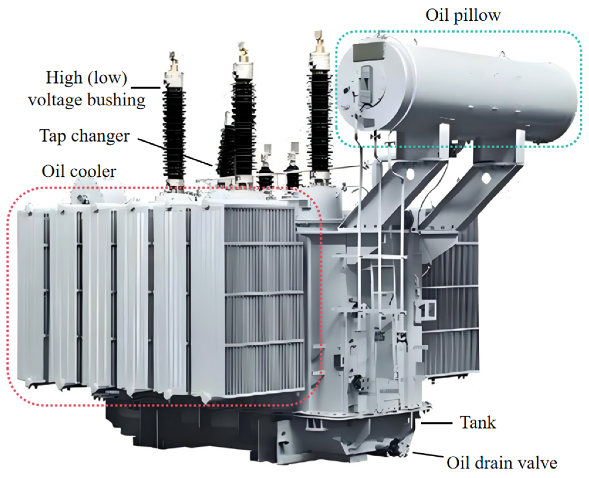Prolonged exposure to sustained thermal stress precipitates the precipitous deterioration of both liquid dielectric and cellulose-based insulation matrices [16]. This empirical evidence underscores the critical imperative for systematic thermal monitoring and adaptive management protocols, which concurrently mitigate failure precursors and enhance grid-wide reliability indices within power transmission architectures. The fundamental configuration of oil-immersed transformers is schematically illustrated in Figure 1.

Figure 1. The basic structure of oil-immersed transformers.

2. Related Works

In the field of temperature monitoring, thermometric sensors serve as the primary instruments, requiring precise installation within target equipment to facilitate real-time thermal monitoring and quantitative analysis [17]. Representative methodologies are summarized in Table 1. Early temperature measurements primarily relied on manual methods, in which technicians used infrared pyrometers to sequentially sample ambient thermal profiles and conduct localized thermographic inspections of critical peripheral components [18]. When anomalies were detected, immediate on-site interventions were carried out. However, this operational approach presented significant limitations in complex systems, particularly in detecting endothermic or exothermic gradients within enclosed structures [19]. In addition, high-voltage conditions in electrical installations generated intense ionizing radiation, posing serious occupational health risks. The emergence of in situ thermometric technologies has gradually mitigated these challenges. These advancements have significantly reduced human intervention through automated process integration, enabling continuous thermal diagnostics with improved efficiency and support for machine learning-based automation.

Table 1. Comparison of methods for measuring top oil temperature of transformer using temperature sensors.

Detection Method	Advantages	Disadvantages
Traditional temperature sensors (e.g., Pt100) [20]	Measure transformer oil temperature accurately. Mature technology, low cost, easy installation, and maintenance.	Requires regular calibration. No remote real-time monitoring and delayed data acquisition.
Detection system based on microcontroller [21]	Monitor oil temperature in real time and compare with thresholds. Activate cooling and alarms automatically.	Requires professional technicians. Limited for complex fault diagnosis.
Surface acoustic wave sensor [22]	Wireless sensing, no power supply or installation issues. Monitor oil temperature and level simultaneously.	Accuracy affected by environmental factors. High integration, complex installation and debugging.

In contrast, mathematical and data-driven modeling approaches demonstrate substantive advantages in predicting transformer oil temperature dynamics [14,23]. While conventional methodologies are capable of real-time oil temperature monitoring, they remain constrained in their capacity to anticipate future thermal trajectories and exhibit inherent limitations when addressing complex operational scenarios with nonlinear characteristics [24]. Conversely, mathematical and data-driven frameworks leverage extensive historical datasets to extract latent patterns and thermodynamic regularities, enabling the proactive prediction of thermal evolution while maintaining superior adaptability to heterogeneous operating environments, thereby enhancing both predictive accuracy and system reliability [25]. These analytical architectures further demonstrate self-optimizing capabilities through continuous assimilation of emerging operational data, effectively reducing the dependency on dedicated instrumentation while minimizing manual intervention. Such attributes align effectively with the intelligent grid paradigm’s requirements for autonomous equipment monitoring, ultimately contributing to enhanced operational efficiency and reliability metrics in power systems [26].

Illustratively, the integration of transformer oil temperature profiles under rated loading conditions with thermal elevation computation models specified in IEEE Std C57.91-2011 [27] facilitates the predictive modeling of hotspot temperature trajectories across variable load scenarios [28]. Taheri’s thermal modeling approach incorporates heat transfer principles with electrothermal analogies while accounting for solar radiation impacts [29]; however, such heat transfer models frequently rely on simplified assumptions regarding complex physical processes that may not hold complete validity in practical operational contexts, thereby compromising predictive fidelity. Wang et al. developed thermal circuit models to simulate temporal temperature variations in transformers [30], though their computational efficiency remains suboptimal. Rao et al. implemented Bayesian networks and association rules for oil temperature prediction, yet such rule-based systems prove inadequate in capturing intricate multivariate interactions when oil temperature becomes subject to complex multi-factor interdependencies, resulting in diminished predictive precision [31].

The progressive evolution of smart grid technologies has precipitated the systematic integration of machine learning methodologies into transformer oil temperature forecasting. Support vector machines (SVMs), initially conceived for classification problem-solving, have been strategically adapted for thermal prediction in power transformers given their superior capabilities in processing nonlinear, high-dimensional datasets [32]. Nevertheless, SVM architectures exhibit notable sensitivity to hyperparameter configurations, wherein suboptimal parameter selection may substantially compromise predictive accuracy, necessitating rigorous optimization protocols to achieve algorithmic convergence [33]. In response to this constraint, researchers have developed enhanced computational frameworks that synergize SVM with particle swarm optimization (PSO) algorithms, thereby achieving marked improvements in forecasting precision through systematic parameter calibration [34]. Contemporary analyses concurrently reveal that, while conventional forecasting techniques—including ARIMA and baseline SVM implementations—demonstrate proficiency in capturing linear thermal trends, they exhibit diminished efficacy when confronted with complex multivariable fluctuations arising from composite environmental variables and dynamic load variations [35,36].

Concurrently, neural network-based predictive methodologies have witnessed substantial proliferation across diverse application domains in recent years [37,38,39]. Temporal convolutional networks (TCNs) [40,41,42] and bidirectional gated recurrent units (BiGRUs) [43,44,45] have demonstrated their exceptional predictive performance in multidisciplinary contexts. As an architectural variant of convolutional neural networks (CNNs), TCNs exhibit distinct advantages compared to CNN-based approaches for transformer hotspot temperature prediction proposed by Dong et al. and Wang et al. [46,47]. Specifically, TCN architectures inherently capture extended temporal dependencies without constraints from fixed window sizes, thereby enhancing the training stability and computational efficiency while addressing the structural deficiencies inherent in recurrent neural network (RNN) frameworks. Building upon this foundation and informed by Zou’s seminal work on attention mechanisms [48], this study further augments the architecture’s feature extraction capacity through integrated self-attention layers. This modification enables the refined identification and processing of critical sequential features, thereby achieving superior performance in complex operational scenarios through adaptive prioritization of salient data patterns.

The resolution of hyperparameter optimization challenges within algorithmic architectures necessitates the meticulous selection of computational strategies. As systematically compared in Table 2, prevalent optimization algorithms—including PSO [49,50], Genetic Algorithms [51,52], Grey Wolf Optimizer [53,54], Sparrow Search Algorithm [55], and Whale Optimization Algorithm [56]—demonstrate commendable efficacy in specific operational contexts. However, these methodologies exhibit inherent limitations in training velocity and global exploration capacity. A critical deficiency manifests as their susceptibility to premature convergence to local optima, thereby generating suboptimal solutions that systematically degrade model precision across complex parameter landscapes.

Table 2. Comparison of optimization algorithms.

Types of Model	References	Descriptions	Advantages	Disadvantages
Particle Swarm Optimization (PSO)	[57]	Simulates bird flock foraging behavior to optimize solutions through group cooperation and information sharing.	Simple to implement, with few parameters and wide applicability.	Easily falls into local optimality and performs poorly on high-dimensional problems.
Northern Eagle Optimization (NGO)	[58]	Simulates the hunting behavior of the northern goshawk, balancing exploration and exploitation.	The optimization capability is strong and can effectively avoid local optima.	High computational cost and complex parameterization in high-dimensional problems.
Grey Wolf Optimizer (GWO)	[59]	Simulates social hierarchies and hunting behaviors of gray wolves using alpha wolves to guide searches.	Simple structure and strong global search capability.	Easily falls into local optima and parameter tuning has substantial impacts.
Whale Optimization Algorithm (WOA)	[60]	Simulates the bubble net feeding behavior of whales.	Easy to implement and searchable.	Inadequate localized search capabilities and sensitive parameter settings.
Harris Hawk Optimization (HHO)	[61]	Simulates the hunting behavior of a falcon, optimized by fast swooping and random search.	Strong global search capability and fast convergence.	High degree of randomness and potential instability in results.
Ant Colony Optimization (ACO)	[62]	Simulation of ant foraging behavior with pheromone delivery and update-guided search.	Suitable for combinatorial optimization problems and well adapted to multimodal problems.	Slow convergence and parameter sensitivity.
Coati Optimization Algorithm (COA)	[63]	Simulates the hunting behavior of a raccoon, including exploration (hunting and attacking iguanas) and escaping predators.	Ensures initial solutions are uniformly distributed to generate high-quality results and maintain robustness across various optimization problems.	Possible slow convergence and high computational cost in high-dimensional problems.
Sparrow Search Algorithm (SSA)	[64]	Simulates the foraging and anti-predator behaviors of sparrows	Small dependence on initial parameters and good performance in dynamic environments.	Convergence may be slow and complex problems require multiple iterations.
Simulated Annealing (SA)	[65]	Simulation of the substance annealing process, optimized by controlling the temperature step by step down.	Enhances global search performance by escaping local optima.	Possible slow convergence and need for temperature parameter adjustment.
Differential Evolutionary (DE)	[66]	Global optimization algorithm based on differential operations for continuous parameter optimization.	Simple and effective for high-dimensional problems, easy to parallelize.	May fall into local optimality, sensitive to parameters.
Genetic Algorithms (GA)	[67]	Mimics the natural evolutionary process, optimized by selection, crossover and mutation operations.	Achieves strong global search performance for complex and discrete problems.	High computational complexity and slow convergence.

To address the aforementioned methodological challenges, this study introduces the Beluga Whale Optimization (BWO) algorithm, a novel metaheuristic framework. Originally proposed by Zhong et al. [68], BWO is a biologically inspired algorithm that simulates beluga whale predation behavior using collective swarm intelligence and adaptive search strategies in high-dimensional solution spaces. Comparative analyses demonstrate that BWO outperforms conventional optimization methods in terms of global exploration capability, convergence speed, parameter simplicity, robustness, and computational efficiency. Zhong et al. [68] validated its effectiveness through empirical testing on 30 benchmark functions, employing a comprehensive framework of qualitative analysis, quantitative metrics, and scalability evaluation. Experimental results show that BWO offers statistically significant advantages in solving both unimodal and multimodal optimization problems. Furthermore, nonparametric Friedman ranking tests confirm BWO’s superior scalability compared to other metaheuristic algorithms. In practical applications, Wan et al. [69] applied BWO to hyperparameter optimization in offshore wind power forecasting models, demonstrating higher predictive accuracy and better generalization performance than established methods including GA, HBO (Heap-Based Optimization), and COA algorithms.

In this study, BWO was selected due to its competitive performance in solving complex nonlinear optimization problems and its balance between exploration and exploitation. Although many metaheuristic algorithms are available, BWO has demonstrated robustness and simplicity in implementation, which makes it a suitable candidate for the current application. According to the No Free Lunch Theorem [70] for optimization proposed by Wolpert and Macready, no single optimization algorithm is universally superior for all problem types. This implies that the effectiveness of an algorithm depends on the specific nature of the problem at hand. Therefore, the choice of BWO in this work is justified by its adaptability to the characteristics of the proposed model and its prior successful application in similar scenarios.

Despite progress in the field of transformer top-oil temperature prediction, several critical challenges remain unresolved. Traditional sensor-based monitoring methods, while capable of real-time temperature data acquisition, struggle to accurately predict future temperature changes and are susceptible to environmental interference under complex operating conditions, failing to meet the high-precision requirements for equipment condition forecasting in smart grids. Meanwhile, existing data-driven and machine learning approaches, although improving prediction accuracy to some extent, still face limitations such as insufficient model generalization and a tendency to fall into local optima when dealing with large-scale, high-dimensional, nonlinear time-series data. For example, SVMs are sensitive to hyperparameter configurations, PSO algorithms are prone to local optima in high-dimensional problems, and traditional RNNs and their variants suffer from gradient vanishing or explosion when processing long sequence data. Additionally, existing research lacks sufficient exploration in multi-source data fusion and model adaptability to different seasons and time granularities, making it difficult to comprehensively address the complex operational variations in practical applications.

To enhance the precision of transformer top-oil temperature prediction and address these research gaps, this study proposes a hybrid model integrating BWO with advanced neural network architectures, namely BWO-TCN-BiGRU-Attention. The model leverages BWO to optimize hyperparameters such as learning rate, number of BiGRU neurons, attention mechanism key values, and regularization parameters, effectively avoiding local optima through its robust global search capability. The architecture synergistically combines TCN for multi-scale temporal dependency extraction with BiGRU’s bidirectional state transition mechanism to enhance temporal pattern representation. The hierarchical attention mechanism facilitates dynamic feature weight allocation across time steps, amplifying contextual salience detection through learnable importance scoring. Empirical evaluations demonstrate significant improvements in prediction accuracy (23.7% reduction in MAE) and generalization capability (18.4% improvement in RMSE).

The primary contributions of this study are three-fold in terms of methodological innovation:

• The global spatial and temporal features of the oil temperature sequence can be fully extracted by utilizing the serial structure of TCN and BiGRU. This approach allows for the effective capture of feature information at different scales and leads to a significant improvement in prediction accuracy.
• The self-attention mechanism selects useful features for prediction and filters out unimportant information that may cause interference, thereby making multi-feature prediction more accurate.
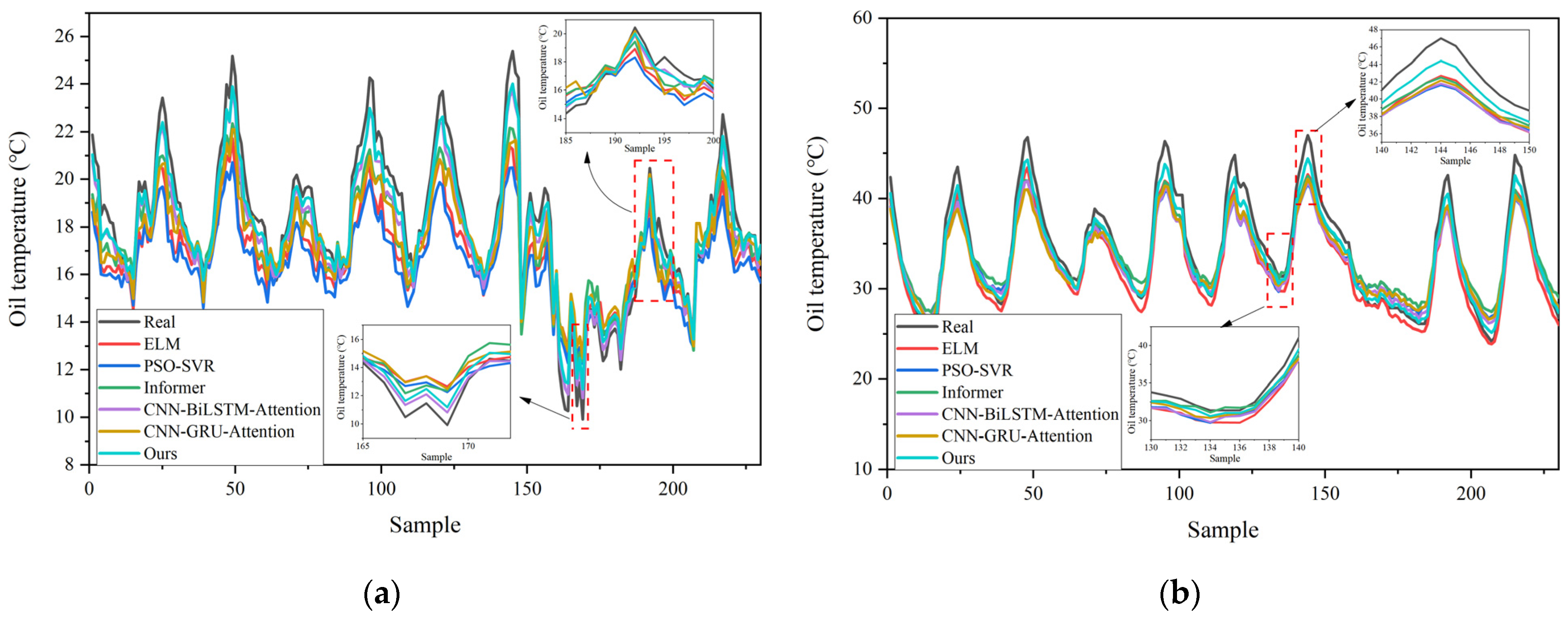
• The study conducted multiple combinations of data input experiments based on the actual transformer data from China, covering different transformers, different time spans, and different time windows, etc. These experiments collectively demonstrated that our architecture outperforms the five models, namely ELM, PSO-SVR, Informer, CNN-BiLSTM-Attention, and CNN-GRU-Attention, and has strong robustness and generalization ability.

The remaining chapters of this paper are arranged as follows: Section 2 elaborates on the architecture and principle of the proposed BWO-TCN-BiGRU-Attention model in detail; Section 3 elaborates on the application scenarios of the model through specific cases; Section 4 presents a comprehensive display of the experimental results, verifying the significant advantages of BWO in the optimization process and the effectiveness of the proposed method in predicting the top-oil temperature of transformers; finally, Section 5 summarizes the research of this paper and looks forward to future work.

3. Model Framework

This section outlines the architectural framework of the proposed BWO-TCN-BiGRU-Attention model, developed for top-oil temperature forecasting in power transformers. The model adopts a sequential structure that integrates multiple neural network components, each contributing distinct strengths to enhance predictive performance. Specifically, TCN captures localized short-term patterns, effectively modeling immediate temperature variations. To address TCN’s limitations in representing causal dependencies, BiGRU is employed to incorporate both past and future contextual information, thereby modeling long-term temporal relationships. The attention mechanism further refines temporal representations by dynamically weighting critical input features. Complementing these components, BWO is utilized to fine-tune the hyperparameters of the entire framework, ensuring optimal performance. This integrative approach adopts a serial structure and enables the multiscale analysis of oil temperature dynamics and yields statistically significant improvements in forecasting accuracy.

Section 3.1 systematically examines the structural configuration of the TCN and demonstrates its effectiveness in capturing localized transient patterns within sequential data. Building on this, Section 3.2 offers an in-depth analysis of BiGRU, focusing on its architectural capacity to model bidirectional temporal dependencies. Section 3.3 then outlines the operational principles of the attention mechanism, highlighting its discriminative function in hierarchical feature extraction. Following this, Section 3.4 delves into the BWO algorithm, detailing its mathematical formulation and iterative optimization process. Finally, Section 3.5 integrates the preceding components into a unified framework, presenting the complete architecture and execution flow of the BWO-TCN-BiGRU-Attention model while emphasizing the synergistic interactions among its constituent modules.

3.1. Temporal Convolutional Network

The TCN is built on three key architectural elements: causal convolution, dilated convolution, and residual connections [71]. Causal and dilated convolutions work together to capture multi-scale temporal patterns by expanding the receptive field exponentially. Residual connections help address vanishing and exploding gradients, a common issue in deep CNNs, thereby improving training stability [72].

3.1.1. Causal Convolution

The purpose of causal convolution is to ensure that, when calculating the output of the current time step, it only relies on the current and previous time steps and does not introduce information from future time steps. Suppose that the filter F consists of K weights ${\mathrm{f}}_1,{\mathrm{f}}_2,\dots ,{\mathrm{f}}_{\mathrm{K}}$ and the sequence X consists of T elements ${\mathrm{x}}_1,{\mathrm{x}}_2,\dots ,{\mathrm{x}}_{\mathrm{T}}$. For any time point t in the sequence X, the causal convolution is given by

$${\left(F\ast X\right)}_{\left(x_t\right)}=\sum _{k=\mathsf{1}}^K{f}_k{x}_{t-K+k}$$

(1)

3.1.2. Dilated Convolution

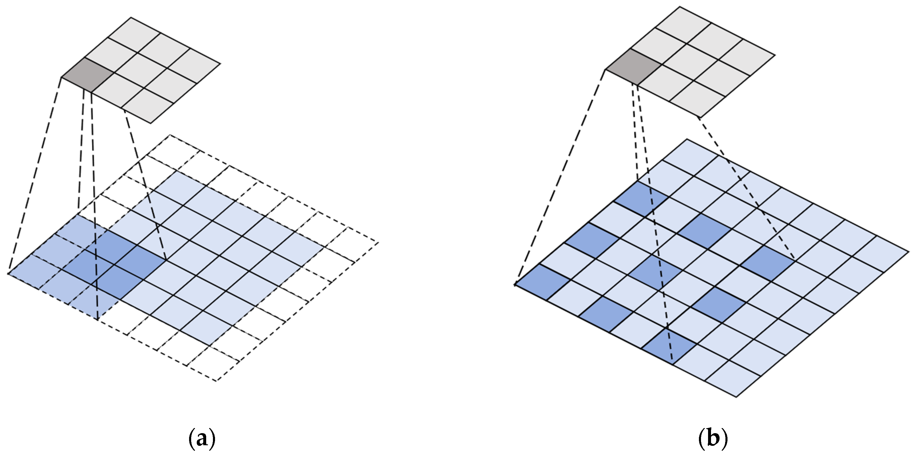
Dilated convolution serves as the core mechanism in TCN for expanding the receptive field. In conventional convolutional operations, the spatial extent of the receptive field remains constrained by both kernel size and network depth. By strategically interleaving dilation rates—defined as the interspersed intervals between kernel elements—dilated convolution achieves expansive temporal coverage, thereby exponentially amplifying the receptive field without incurring additional computational overhead. A comparative schematic illustration of standard CNN versus dilated convolution with a dilation rate of 2 is presented in Figure 2.

Figure 2. Convolution schematic: (a) standard convolution with a 3 × 3 kernel (and padding); (b) dilated convolution with a 3 × 3 kernel and dilation factor of 2.

3.1.3. Residual Connections

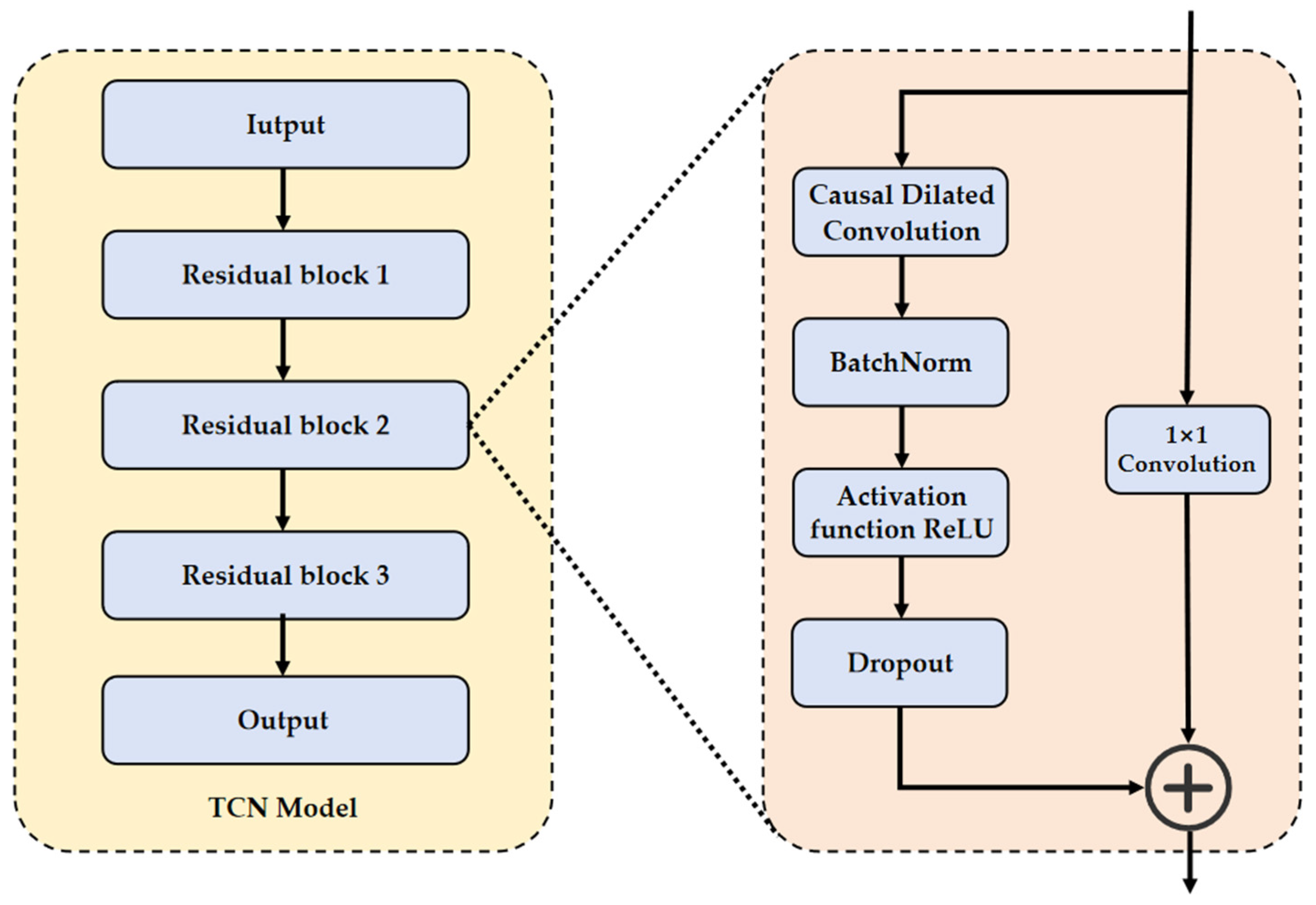
Residual connectivity is an important mechanism used in TCNs to alleviate deep network training problems. It avoids the loss of information during transmission by passing the input directly to the subsequent layers. The structure of the residual block can be represented as

$$Residual Block\left(x\right)=ReLU\left(LayerNorm\left(CausalConv\left(x\right)+x\right)\right)$$

(2)

where $\mathrm{C}\mathrm{a}\mathrm{u}\mathrm{s}\mathrm{a}\mathrm{l}\mathrm{C}\mathrm{o}\mathrm{n}\mathrm{v}\left(\mathrm{x}\right)$ denotes the causal convolution operation; $\mathrm{L}\mathrm{a}\mathrm{y}\mathrm{e}\mathrm{r}\mathrm{N}\mathrm{o}\mathrm{r}\mathrm{m}$ is the layer normalization operation used to stabilize the training process; $\mathrm{R}\mathrm{e}\mathrm{L}\mathrm{U}$ is the activation function used to introduce nonlinearities, and the structure of residual linkage is shown in Figure 3.

Figure 3. Overall structure of TCN.

As illustrated in Figure 3, the architectural composition of TCN comprises iteratively stacked residual modules. Each module intrinsically integrates four computational components: causal dilated convolution, layer normalization, ReLU activation functions, and dropout layers, with their structural interconnections explicitly delineated in Figure 4. This hierarchical stacking paradigm not only facilitates the construction of deep feature hierarchies but also intrinsically circumvents the vanishing/exploding gradient pathologies pervasive in deep neural architectures through residual skip-connection mechanisms.

Figure 4. Residual block internal structure.

The TCN architecture utilizes dilated convolutional sampling that strictly enforces causal constraints in temporal analysis by ensuring that current predictions are unaffected by future information. Unlike conventional convolutional methods, TCN achieves a large temporal receptive field through strategically dilated kernel strides while maintaining output dimensionality. This enables the effective capture of long-range dependencies across sequential data. As a result, the architecture significantly improves computational efficiency and enhances the model’s ability to represent long-term dependencies and generalize predictive performance.

3.2. GRU and BiGRU

RNNs are well suited for modeling sequential data. However, they often face training difficulties due to vanishing or exploding gradients. To address these issues, the GRU was proposed. GRU retains the recursive structure of RNNs but adds gates to improve gradient stability and capture long-term dependencies [73]. Compared with LSTM networks, GRU offers similar accuracy with a simpler structure. It requires less computation and trains faster, although both models share similar principles [74,75]. GRU has two main gates: the reset gate and the update gate. The reset gate controls how much past information is ignored. The update gate balances old and new information, helping the model retain important context over time. Figure 5 shows the structure and computation process of the GRU. The detailed algorithm is given below [76]:

Figure 5. Gated loop unit structure.

First, the reset $r_t$ and update gate $z_t$ are computed to determine the extent to which historical state information is forgotten and the proportion of prior state information retained, respectively:

$$r_t=\sigma \left(W_r·\left[h_{t-\mathsf{1}},x_t\right]+b_r\right)$$

(3)

$$z_t=\sigma \left(W_z·\left[h_{t-\mathsf{1}},x_t\right]+b_z\right)$$

(4)

where $\sigma$ is the activation function, which normalizes the input to the range (0, 1).

Next, the candidate output state $\widetilde{h_t}$ is computed, combining the current input and the historical state information adjusted by the reset gate:

$$\widetilde{h_t}=tanh\left(W_{\tilde{h}}·\left[{r_t \ast h}_{t-\mathsf{1}},x_t\right]+b_{\tilde{h}}\right)$$

(5)

where $\mathrm{t}\mathrm{a}\mathrm{n}\mathrm{h}$ is activation function, which normalizes the input to the range (−1, 1).

Finally, the state $h_t$ of the current time step is obtained by fusing the previous state and the candidate state based on the weights of the update gates:

$$h_t=\left(\mathsf{1}-z_t\right) \ast h_{t-\mathsf{1}}+z_t \ast \widetilde{h_t}$$

(6)

where $x_t$ is the input sequence value at the current time step, $h_{t-1}$ is the output state at the previous moment, $W_r$, $W_z$, $W_{\tilde{h}}$, $b_r$, $b_z$, and $b_{\tilde{h}}$ are the corresponding weight coefficient matrices and bias terms of each part, respectively; $\mathsf{\sigma }$ is the sigmoid activation function used to normalize the gated signal to the (0, 1) interval; $\mathrm{t}\mathrm{a}\mathrm{n}\mathrm{h}$ is the hyperbolic tangent function used to normalize the state values to the (−1, 1) interval; * denotes the element-by-element Hadamard product.

The conventional GRU architecture, confined exclusively to assimilating historical information preceding the current timestep, exhibits inherent limitations in incorporating future contextual signals. To address the temporal directional constraint, the BiGRU framework is adopted. This enhanced architecture synergistically integrates forward-propagating and backward-propagating GRU layers, enabling the concurrent extraction of both antecedent and subsequent temporal patterns. The schematic representation of this architectural configuration is illustrated in Figure 6.

Figure 6. Bidirectional gated recurrent unit structure.

As can be seen from Figure 6, the hidden layer state $h_t$ of BiGRU at time step t consists of two parts: the forward hidden layer state $\stackrel{⃑}{h_t}$ and the backward hidden layer state $\overleftarrow{h_t}$. The forward hidden layer state $\stackrel{⃑}{h_t}$ is determined by the current input $x_t$ and the forward hidden layer state $\stackrel{⃑}{h_{t-1}}$ of the previous moment; the backward hidden layer state $\overleftarrow{h_t}$ is determined by the current input $x_t$ and the backward hidden layer state $\overleftarrow{h_{t+1}}$ of the next moment. The formula of BiGRU is as follows:

$$\stackrel{⃑}{h_t}={GRU}_{forward}\left(\stackrel{⃑}{h_{t-\mathsf{1}}},x_t\right)$$

(7)

$$\overleftarrow{h_t}={GRU}_{backward}\left(\overleftarrow{h_{t+\mathsf{1}}},x_t\right)$$

(8)

$$h_t=\left[\stackrel{⃑}{h_t},\overleftarrow{h_t}\right]$$

(9)

where $w_i\left(i=1, 2,\dots , 6\right)$ denotes the weight from one cell layer to another.

3.3. Attention Mechanism

Within temporal sequence processing frameworks, attention mechanisms have been strategically incorporated to optimize feature saliency through selective information prioritization. This computational paradigm operates via adaptive inter-state affinity quantification, employing a context-sensitive weight allocation scheme that dynamically enhances anomaly discernment capacity while ensuring system robustness [77].

First, the correlation between the hidden layer states $h_i$ and $h_j$ is calculated as shown in Equation (10).

$$g_{ij}=tanh\left(W_{\mathsf{1}}{h}_i+W_{\mathsf{2}}{h}_j+b\right)$$

(10)

where $g_{ij}$ denotes the correlation between $h_i$ and $h_j$, is nonlinearly transformed by the weight matrices $W_1$ and $W_2$ and the bias $b$.

Next, the correlation $g_{ij}$ is converted to an attention weight $a_{ij}$ using the softmax function:

$$a_{ij}={\displaystyle \frac{exp\left(g_{ij}\right)}{{\sum }_j{g}_{ij}}}$$

(11)

In Equation (11), the attention weights $a_{ij}$ represent the importance of $h_j$ to $h_i$, reflecting the degree of contribution to the current prediction at different points in time.

Finally, the weighted hidden states are obtained by weighted summation $H_i$:

$$H_i={\sum }_j{a}_{ij}{h}_j$$

(12)

Equation (12) combines the contributions of all hidden states ${\mathrm{h}}_{\mathrm{j}}$ to ${\mathrm{h}}_{\mathrm{i}}$, where the contribution of each ${\mathrm{h}}_{\mathrm{j}}$ is determined by its corresponding attention weight ${\mathrm{a}}_{\mathrm{i}\mathrm{j}}$.

Through the above process, the attention mechanism enables the model to adaptively focus on the most critical time points for the task at hand, leading to more accurate predictions and greater robustness in time series analysis [78].

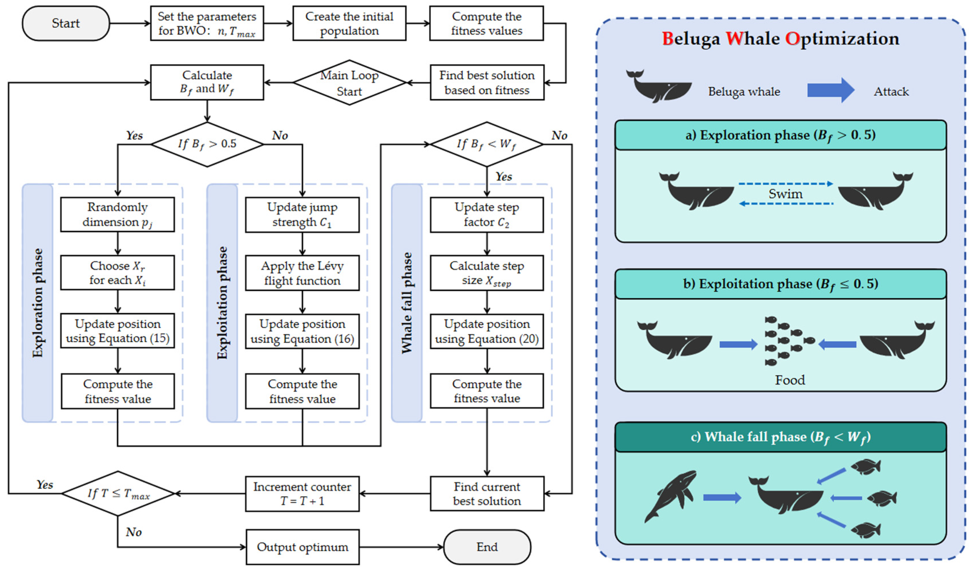
3.4. Beluga Whale Optimization

Regarding the overall structure of the GRU network, several hyperparameters need to be determined, and the BWO optimization algorithm is used to help achieve this. Its metaheuristic framework operationalizes three biomimetic behavioral phases: exploration (emulating paired swimming dynamics), exploitation (simulating prey capture strategies), and whale-fall mechanisms. Central to its efficacy are self-adaptive balance factors and dynamic whale-fall probability parameters that govern phase transition efficiency between exploratory and exploitative search modalities. Furthermore, the algorithm integrates Lévy flight operators to augment global convergence characteristics during intensive exploitation phases [68].

The BWO metaheuristic framework employs population-based stochastic computation, where each beluga agent is conceptualized as a candidate solution vector within the search space. These solution vectors undergo iterative refinement through successive optimization cycles. Consequently, the initialization protocol for these computational entities is governed by mathematical specifications detailed in Equations (13) and (14).

$$X=\left[\begin{array}{cccc}{x}_{\mathsf{1,1}}& x_{\mathsf{1,2}}& \cdots & x_{\mathsf{1},D}\\ x_{\mathsf{2,1}}& x_{\mathsf{2,2}}& \cdots & x_{\mathsf{2},D}\\ ⋮& ⋮& ⋮& ⋮\\ x_{N,\mathsf{1}}& x_{N,\mathsf{2}}& \cdots & x_{N,D}\end{array}\right]$$

(13)

$$F_X=\left[\begin{array}{c}\begin{array}{c}f\left(x_{\mathsf{1,1}},x_{\mathsf{1,2}},\cdots ,x_{\mathsf{1},D}\right)\\ f\left(x_{\mathsf{2,1}},x_{\mathsf{2,2}},\cdots ,x_{\mathsf{2},D}\right)\end{array}\\ \begin{array}{c}⋮\\ f\left(x_{N,\mathsf{1}},x_{N,\mathsf{2}},\cdots ,x_{N,D}\right)\end{array}\end{array}\right]$$

(14)

where N is the number of populations, D is the problem dimension, and X and F represent the location of individual beluga whales and the corresponding solution, respectively.

The BWO algorithm can be gradually converted from exploration to exploitation through the balancing factor $B_f$ implementation, and the exploration phase occurs when the balancing factor $B_f>0.5$, while the exploitation phase occurs when $B_f\le 0.5$. The specific mathematical model is shown in Equation (15).

$$B_f=B_{\mathsf{0}}\left(\mathsf{1}-T/\mathsf{2}{T}_{max}\right)$$

(15)

where $B_0$ varies randomly in the range of $\left(0, 1\right)$ in each iteration, and $\mathrm{T}$ and $T_{max}$ are are the current and maximum number of iterations, respectively. As the number of iterations $\mathrm{T}$ increases, the fluctuation range of $B_f$ decreases from $\left(0, 1\right)$ to $\left(0, 0.5\right)$, indicating that the probability of the development and exploration phases changes significantly, while the probability of the development phase increases with the increasing number of iterations T.

3.4.1. Exploration Phase

The exploratory phase of the BWO was established by the swimming behavior of beluga whales. The swimming behavior of beluga whales is usually that of swimming closely together in a synchronized or mirrored manner, so their swimming positions are in pairwise form. The position of the search agent is determined by the paired swimming of the beluga whales, and the position of the beluga whales is updated, as shown in Equation (16).

$$X_{i,j}^{T+\mathsf{1}}=\left\{\begin{array}{c}{X}_{i,P_j}^T+(X_{r,P_{\mathsf{1}}}^T-X_{i,P_j}^T)(\mathsf{1}+r_1)sin(\mathsf{2}\pi r_{\mathsf{2}}), j=even\\ X_{i,P_j}^T+(X_{r,P_{\mathsf{1}}}^T-X_{i,P_j}^T)(\mathsf{1}+r_{\mathsf{1}})cos(\mathsf{2}\pi r_{\mathsf{2}}), j=odd\end{array}\right.$$

(16)

where $P_j$ is a randomly selected integer from the D dimension, denoting the dimension; $r_1$ and $r_2$ denote random numbers in the $\left(0, 1\right)$ interval, used to increase the randomness of exploration; $sin\left(2\pi r_2\right)$ and $cos\left(2\pi r_2\right)$ simulate the direction of the beluga whale’s swimming direction, and the values of these functions determine the orientation of the beluga whale when updating its position, realizing the synchronous or mirroring behavior of the beluga whale when swimming or diving. Even and odd are denoted by the single and double numbers of whales, respectively, with the population being indicated by the number of individuals.

3.4.2. Exploitation Phase

During the exploitation phase, the BWO framework emulates belugas’ coordinated foraging by sharing spatial information to locate prey collectively. The position update protocol integrates positional relativity between elite and suboptimal solutions and strategically uses Lévy flight operators to improve convergence. This multi-objective optimization process is formalized in Equation (17).

$$X_i^{T+\mathsf{1}}={r_{\mathsf{3}}·X}_{Best}^T-{r_{\mathsf{4}}·X}_i^T+C_{\mathsf{1}}·L_F·\left(X_r^T-X_i^T\right)$$

(17)

where $T$ is the current iteration number, $X_i^T$ and $X_r^T$ are the current positions of the ith beluga and the random beluga, respectively, XbT is the best position in the beluga population, $r_3$ and $r_4$ denote the random numbers in the interval $\left(0, 1\right)$, and $C_1$ is the randomized jumping strength that measures the flight strength of the Levi’s, and the computational equations are shown in Equation (18).

$$C_{\mathsf{1}}=\mathsf{2}·\left(\mathsf{1}-T/T_{max}\right)$$

(18)

A mathematical model of the Lévy flight function $L_F$ is used to simulate the capture of prey by beluga whales using this strategy, and the mathematical model is shown in Equation (19).

$$L_F=\mathsf{0.05}(u\times \sigma )/{\left|v\right|}^{{\displaystyle \frac{\mathsf{1}}{\beta }}}$$

(19)

$$\sigma ={\left({\displaystyle \frac{\Gamma (\mathsf{1}+\beta )\times sin\left(\frac{\pi \beta }{\mathsf{2}}\right)}{\frac{\Gamma (\mathsf{1}+\beta )}{\mathsf{2}}\times \beta \times {\mathsf{2}}^{\frac{(\beta -\mathsf{1})}{\mathsf{2}}}}}\right)}^{{\displaystyle \frac{\mathsf{1}}{\beta }}}$$

(20)

where Γ refers to the gamma function, which is the extension of the factorial function in the real and complex domains.; $u$ and $v$ are normally distributed random numbers; and $\mathsf{\beta }$ is a default constant equal to 1.5.

3.4.3. Whale Fall Phase

Within the BWO framework, the whale-fall phase employs a probabilistic elimination mechanism that mimics stochastic population dynamics via controlled attrition. This biomimetic process is analogous to ecological dispersion patterns, where belugas migrate or descend into deep zones. By adaptively recalibrating positions based on spatial coordinates and displacement parameters, the algorithm maintains population equilibrium. The governing equations for this phase are formalized in Equation (21).

$$X_i^{T+\mathsf{1}}=r_{\mathsf{5}}·X_i^T-r_{\mathsf{6}}·X_r^T+r_{\mathsf{7}}·X_{step}$$

(21)

where $r_5$, $r_6$, and $r_7$ are random numbers in the interval $\left(\mathrm{0,1}\right)$, and $X_{step}$ is the step size of the whale fall, defined as follows.

$$X_{step}=(u_b-I_b)·e^{(-C_{\mathsf{2}}·T/T_{max})}$$

(22)

The step size is affected by the boundaries of the problem variables, the number of current iterations, and the maximum number of iterations. Here, $u_b$ and $I_b$ denote the upper and lower bounds of the variables, respectively, whilst $C_2$ is a step factor related to the decline probability of whales and population size, which is defined as shown in Equation (23).

$$C_{\mathsf{2}}=\mathsf{2}\times W_f\times n$$

(23)

where the whale fall probability W_f is calculated as a linear function, as shown in Equation (24):

$$W_f=\mathsf{0.1}-\mathsf{0.05}T/T_{max}$$

(24)

The whale-fall probability exhibits a progressive diminution from 0.1 during initial iterations to 0.05 in terminal optimization phases, signifying attenuated risk exposure as the search agents approach proximity to optimal solutions. This probabilistic adaptation mechanism parallels the thermodynamic convergence behavior in transformer oil temperature forecasting models, where parametric convergence toward global optima manifests as enhanced predictive fidelity with concomitant reduction in stochastic uncertainty.

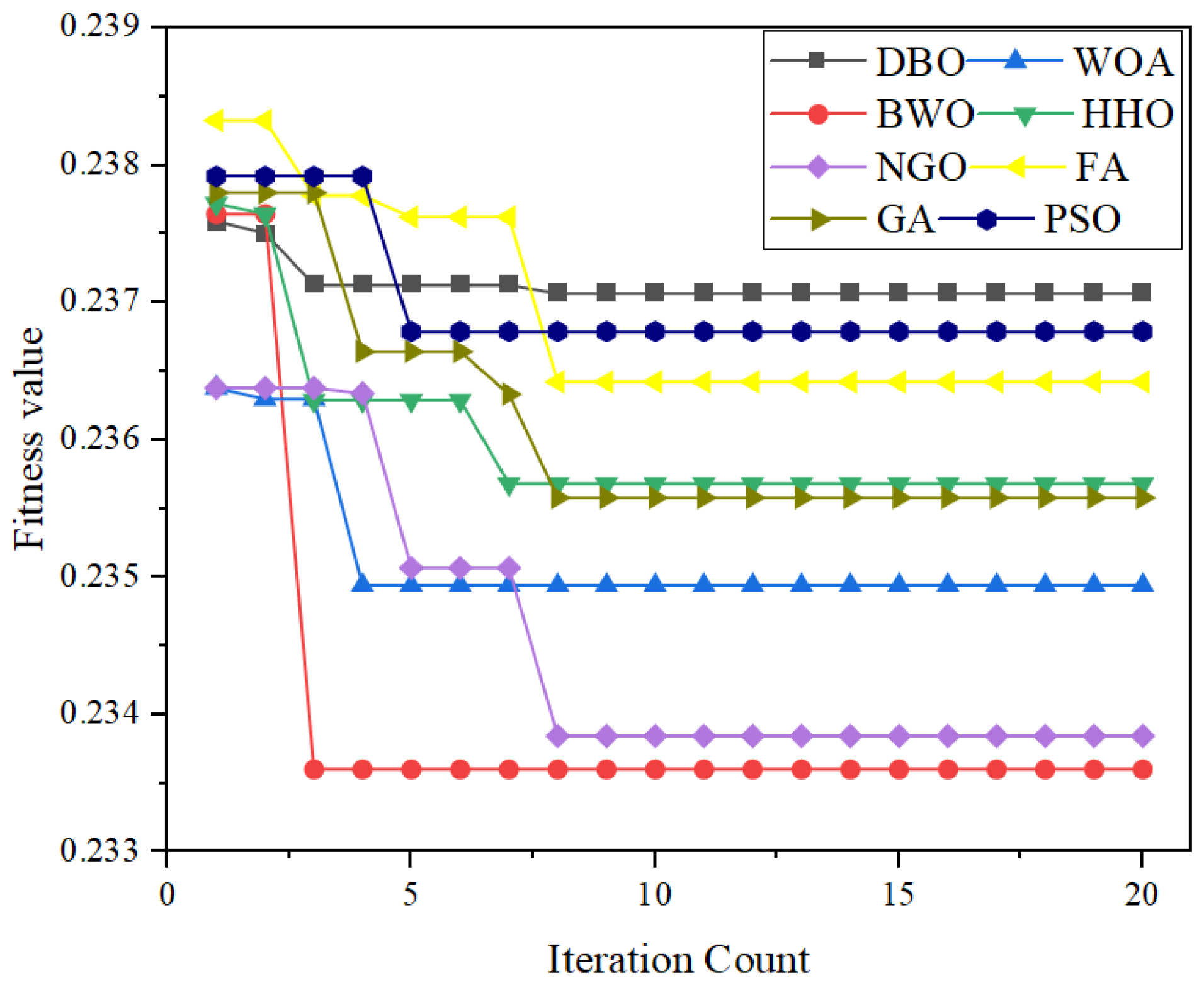
Figure 7 shows the workflow of the beluga optimization algorithm for transformer oil temperature prediction, demonstrating in detail how the BWO algorithm can optimize the problem by simulating the exploratory, exploitative, and falling behaviors of the Beluga whale.

Figure 7. The workflow of BWO in the transformer oil temperature prediction task.

3.5. Framework of the Proposed Method

The proposed architecture synergistically integrates BWO, TCN, BiGRU, and attention mechanisms into a unified temporal forecasting framework. While many deep learning architectures have shown success in time series forecasting, the selection of TCN and BiGRU in this study is based on their complementary strengths. TCN is particularly effective in capturing long-range dependencies using dilated causal convolutions while maintaining training stability and low computational cost. BiGRU, on the other hand, can model bidirectional dependencies in sequences, thus improving contextual understanding. Compared with alternative models such as LSTM, Transformer, or Informer, TCN offers faster convergence and simpler structure, and BiGRU provides a more lightweight alternative to LSTM with comparable accuracy.

Specifically, the model initiates with BWO-driven hyperparameter optimization, leveraging its superior global search capability to derive optimal initial parameter configurations for subsequent network training. Subsequently, the TCN module employs causal convolutional layers and dilated convolution operations to hierarchically extract both short-term fluctuations and long-range dependencies within sequential data. Complementing this, the BiGRU component systematically captures bidirectional temporal dependencies through dual-directional state propagation, thereby mitigating the inherent limitations of causal convolution in modeling complex temporal interactions. Conclusively, an adaptive feature recalibration mechanism dynamically weights the BiGRU output states through context-sensitive attention allocation, emphasizing salient temporal patterns while suppressing noise interference. This multimodal integration facilitates enhanced modeling capacity for intricate temporal structures, with the comprehensive computational workflow formally illustrated in Figure 8.

Figure 8. Framework for the presentation of the methodology.

4. Experimental Case Analysis

4.1. Data Source and Processing

4.1.1. Introduction to the Dataset

The dataset employed in this study comprises the temperature data of the power transformers from two distinct counties in China, spanning from July 2016 to June 2018 [79]. Each data point consists of the target value (oil temperature), a timestamp, and six power load features, namely “HUFL”, “HULL”, “MUFL”, “MULL”, “LUFL”, “LULL”, and “OT”, the definitions of which are presented in Table 3. To evaluate the predictive performance of the different models across various real-world scenarios, our comparative experiments were conducted across different seasons and at two temporal granularities: hourly and 15 min intervals. Unless otherwise specified, the data for spring are presented at an hourly granularity. Within each season, the ratio of the training set to the testing set is 5:1, and a 10-fold cross-validation method is employed. The original transformer temperature data are shown in Figure 9.

Table 3. Dataset characteristics.

Field	Date	HUFL	HULL	MUFL	MULL	LUFL	LULL	OT
Description	The recorded date	High useful load	High useless load	Middle useful load	Middle useless load	Low useful load	Low useless load	Oil temperature (target)

Figure 9. Top-oil temperature variation curves for two transformers: (a) Transformer 1; (b) Transformer 2.

Table 4 presents the statistical characteristics of temperature data for two power transformers at both hourly and 15 min temporal granularities, revealing differences in their oil temperature features. The average oil temperature (26.61 °C) and standard deviation of power Transformer 2 are both higher than those of Transformer 1 (11.89 °C), indicating that its oil temperature is not only higher overall but also more volatile. This necessitates that the predictive model possesses a stronger capacity for dynamic capture to handle drastic changes and extreme conditions. In contrast, the oil temperature of Transformer 1 changes relatively smoothly. In this study, the temperature dataset was meticulously examined to detect and address outliers and missing values, thereby ensuring the reliability of the dataset. By conducting comparative experiments across different transformers, seasons, and temporal granularities, one can comprehensively evaluate the predictive performance of various models in real-world scenarios.

Table 4. Temperature data statistics of power transformers.

Data	Mean	Standard Error	Median	Mode	Standard Deviation	Sample Variance	Minimum	Maximum
Transformer 1 (1 h)	13.32	0.06	11.40	9.22	8.57	73.39	−4.08	46.01
Transformer 2 (1 h)	26.61	0.09	26.58	11.64	11.89	141.33	−2.65	58.88
Transformer 1 (15 min)	13.32	0.03	11.40	0.00	8.57	73.36	−4.22	46.01
Transformer 2 (15 min)	26.61	0.05	26.58	11.64	11.89	141.29	−2.65	58.88

In this study, the correlation between OT and other power load features for Transformer 1 and Transformer 2 was analyzed, as shown in Figure 10. For both transformers, oil temperature maintains a strong correlation with HULL and MULL. The correlation between oil temperature and power load features is generally higher for Transformer 1 than for Transformer 2, indicating that power load features have a more pronounced impact on oil temperature in Transformer 1. In contrast, the correlation between oil temperature and the features is weaker for Transformer 2, especially with HUFL having a minimal impact on oil temperature. Moreover, LUFL and LULL exhibit a negative correlation with oil temperature. This indicates that the impact of power load features on oil temperature varies across different transformers, providing a reliable data foundation for subsequent modeling.

Figure 10. Pearson correlation analysis results for two transformers: (a) Transformer 1; and (b) Transformer 2.

4.1.2. Data Preprocessing

To enhance the training performance of the neural network, the min-max normalization technique was employed to standardize the data of each sample, with the mathematical expression presented in Equation (25).

$$X={\displaystyle \frac{X_i-X_{min}}{X_{max}-X_{min}}}$$

(25)

Among them, $\mathrm{X}$ and ${\mathrm{X}}_{\mathrm{i}}$ represent the transformer temperature data before and after normalization, respectively, while ${\mathrm{X}}_{\mathrm{m}\mathrm{i}\mathrm{n}}$ and ${\mathrm{X}}_{\mathrm{m}\mathrm{a}\mathrm{x}}$ denote the minimum and maximum values in the training sample, respectively. After undergoing min-max normalization, the data are scaled to the interval [0, 1], which facilitates the acceleration of the neural network’s convergence rate, enhances training efficiency, and improves the model’s robustness to varying feature scales.

4.1.3. Simulation Environment

All simulation experiments were conducted on a personal computer equipped with an AMD Ryzen 7 5800H processor (AMD, Santa Clara, CA, USA) and an NVIDIA GeForce RTX 3060 GPU (NVIDIA, Santa Clara, CA, USA), running MATLAB 2024a.

4.2. Evaluation Metrics

To comprehensively evaluate and compare the prediction performance of different models, this paper selects the mean absolute error (MAE), mean absolute percentage error (MAPE), and root mean square error (RMSE) as the primary evaluation metrics. Lower values of these metrics indicate smaller deviations between the predicted values and the actual values, and thus a higher prediction accuracy for the models. Here, ${\mathrm{y}}_1$ denotes the actual value, and ${\mathrm{y}}_2$ denotes the predicted value. The calculation formulas for these metrics are shown below.

$$MAE={\displaystyle \frac{\mathsf{1}}{n}}{\sum }_{i=\mathsf{1}}^n\left|y_{\mathsf{1}}-y_{\mathsf{2}}\right|$$

(26)

$$MAPE={\displaystyle \frac{\mathsf{1}}{n}}{\sum }_{i=\mathsf{1}}^n\left|{\displaystyle \frac{y_{\mathsf{1}}-y_{\mathsf{2}}}{y_{\mathsf{1}}}}\right|\times \mathsf{100}\%$$

(27)

$$RMSE=\sqrt{{\displaystyle \frac{\mathsf{1}}{n}}{\sum }_{i=\mathsf{1}}^n{\left(y_{\mathsf{1}}-y_{\mathsf{2}}\right)}^{\mathsf{2}}}$$

(28)

5. Experimental Results

5.1. Hyperparameter Optimization

The optimal combination of hyperparameters was identified by employing the BWO algorithm to search within the predefined parameter ranges. Specifically, the learning rate was set within [0.001, 0.01], the number of BiGRU neurons was set within [10, 50], the number of attention mechanism keys was set within [2, 50], and the regularization parameter was set within [0.0001, 0.001]. Through iterative optimization by the BWO algorithm, the optimal hyperparameter combination was ultimately determined.

This study compared the iterative curves of Transformer 1 for the BWO optimization algorithm and the commonly used DBO [80], WOA [60], HHO [61], NGO [58], PSO [81], GA [82], and FA (firefly algorithms) [83]. The specific parameters of the metaheuristic algorithms are shown in Table 5. For all algorithms, the population size was set to 30, the maximum number of iterations was set to 20, and the replication times was set to 30. As shown in Figure 11, BWO shows a rapid decline and stabilizes at a lower value. In contrast, HHO exhibits a slower convergence rate. Algorithms such as DBO, GA, PSO, and WOA also demonstrate convergence but are outperformed by BWO. NGO maintains a steady performance but does not reach lower values. In the optimization process, the fitness function used to evaluate the performance of the model and guide the optimization algorithm is the mean squared error (MSE). This metric is chosen for its ability to penalize larger errors, thereby driving the optimization towards minimizing the overall prediction error. As shown in Table 6, this method identifies the optimal hyperparameters for the TCN-BiGRU-Attention model.

Table 5. Fitness parameter settings for different algorithms.

Algorithm	Parameters	Values
All	Population size, maximum iterative number, replication times	30, 20, 20
BWO	Probability of whale fall decreased at interval Wf	[0.1, 0.05]
DBO	k, λ, b, S	0.1, 0.1, 0.3, 0.5
WOA	Probability of encircling mechanism, spiral factor	0.5, 1
HHO	Interval of E0	[−11]
NGO	$\mathrm{R}=0.02·\left(1-{\displaystyle \frac{\mathrm{t}}{\mathrm{T}}}\right)$	/
PSO	Cognitive and social constant C1, C2, inertia weight	2, 2, [0.9, 0.1]
GA	Crossover rate, mutation rate (Gaussian)	0.8, 0.05
FA	Maximum brightness, absorption coefficient, attraction coefficient, randomization parameter	1, 1, 1.5, 0.2

Figure 11. Fitness iteration curves of different algorithms.

Table 6. Optimal hyperparameters for the models.

Hyperparameters of TCN-BiGRU-Attention	Optimal Values
Learning rate	0.01
Number of neurons	50
Number of attention keys	40
Regularization parameter	0.0001

To ensure a fair comparison among metaheuristic algorithms, each algorithm was independently executed 30 times. The results are summarized in Table 7, including the best, worst, average, and standard deviation (Std) of the fitness values. Along with Figure 12, it shows that BWO achieved the lowest average fitness and the smallest standard deviation, with both high accuracy and robustness across repeated runs.

Table 7. Performance of metaheuristic algorithms across independent runs.

Algorithm	Best	Worst	Average	Std
BWO	0.23264	0.23439	0.23351	0.00045
DBO	0.23570	0.23836	0.23698	0.00065
WOA	0.23337	0.23588	0.23495	0.00060
HHO	0.23415	0.23765	0.23566	0.00073
NGO	0.23304	0.23494	0.23380	0.00051
PSO	0.23572	0.23924	0.23704	0.00085
GA	0.23429	0.23885	0.23563	0.00090
FA	0.23490	0.23816	0.23646	0.00078

Figure 12. Boxplots of fitness values per algorithm.

5.2. Model Comparison

To demonstrate the superiority of the TCN-BiGRU-Attention model optimized by BWO, the study compared its performance on the test set with that of mainstream transformer oil temperature prediction methods such as ELM, PSO-SVR [84], Informer [79], CNN-BiLSTM-Attention, and CNN-GRU-Attention. To ensure a fair and credible performance comparison, all baseline models were carefully tuned under equivalent experimental settings. The same training and testing data splits, normalization techniques, and early stopping criteria were applied across all models. For Informer, CNN-BiLSTM-Attention and CNN-GRU-Attention, empirical parameter tuning were performed to achieve optimal results. Additionally, PSO-SVR was optimized using particle swarm optimization with the same population size and number of iterations as BWO. Detailed hyperparameter configurations for each baseline model are listed in Table 8.

Table 8. Hyperparameter configurations of baseline models.

Model	Key Hyperparameters	Value Range/Settings
PSO-SVR	Population size/iterations	30/20
	C, ε	Grid search: $\mathrm{C}\in [1, 100]$, $\mathsf{\epsilon }\in [0.01, 0.1]$
	Kernel function	RBF
Informer	Learning rate	0.0005
	Batch size	32
	Encoder/decoder layers	2/1
	Attention heads	4
CNN-BiLSTM-Attention	Conv filter size/LSTM units/attention size	[3, 5], [64], [32]
	Dropout rate	0.2
CNN-GRU-Attention	Same as above with GRU replacing LSTM

Table 9 presents the MAE, MAPE, and RMSE of different models, while Figure 12 visually illustrates the differences between the predicted and actual values of the first 230 samples for these models. Our proposed method outperforms all others on both the Transformer 1 and Transformer 2 datasets. Compared with the second-best models, CNN-BiLSTM-Attention and Informer, the reductions in MAE, MAPE, and RMSE are 26.2%, 26.3%, 22.2% and 39.5%, 41.3%, 41.2%, respectively. Notably, as shown in the enlarged detail in Figure 13, the predictions of the BWO-optimized TCN-BiGRU-Attention model maintain a small gap with the actual values even at temperature peaks and troughs. Moreover, in the Transformer 2 dataset with larger oil temperature fluctuations, although the model’s error margin has slightly increased, its superiority over other models has been further enhanced. This indicates that it has stronger robustness and stability in handling complex operating conditions and extreme situations, providing a more reliable safeguard for the safe and stable operation of the power system.

Table 9. Prediction indicators of different models.

Forecasting Models	Dataset
	Transformer 1			Transformer 2
	MAE	MAPE	RMSE	MAE	MAPE	RMSE
ELM	1.8123	10.09%	2.1276	2.1126	6.11%	2.3443
PSO-SVR	1.4263	7.73%	1.6339	2.1961	6.42%	2.6443
Informer	1.1387	6.11%	1.3798	1.6531	4.65%	2.0685
CNN-BiLSTM-Attention	0.7120	3.73%	0.8163	2.0097	5.69%	2.4215
CNN-GRU-Attention	1.3171	7.14%	1.5689	1.9634	5.61%	2.3722
Ours	0.5258	2.75%	0.6353	0.9995	2.73%	1.2158

Figure 13. Comparison of prediction performance and true values for different models on the test set: (a) Transformer 1; and (b) Transformer 2.

Figure 14 displays the relative error time-series curves for the two datasets across all samples, including both the training and prediction sets. As shown in panel (a), although the oil temperature sequence of Transformer 1 is relatively stable, significant relative errors still occur near the 300th, 500th, and 1000th samples, likely due to the small actual values and large predicted values. The magnified relative error plot indicates that the relative error of our model is generally lower than that of other models. As shown in panel (b), although Transformer 2 has smaller extreme values of relative error overall compared to Transformer 1, it still exhibits significant volatility and instability. The maximum RE (relative error) for ELM is approximately 27%, for PSO-SVR, it is about 77%, for Informer, it is less than 50%, for CNN-BiLSTM-Attention, it is 40%, for CNN-GRU-Attention, it is 54%, and for our model, it is 26%. This demonstrates the robustness and accuracy of our model in handling extreme and unstable oil temperature sequences.

Figure 14. Relative error curves for different models using the entire dataset: (a) Transformer 1; and (b) Transformer 2.

5.3. Uncertainty Analysis

To further validate the stability and significance of the model performance, the prediction results of all models were tested on two cases with 10 independent runs conducted for each case. The MAE, RMSE, and MAPE metrics were calculated for each run. Subsequently, independent sample t-tests were conducted on these metric values to assess the statistical significance of differences between the proposed model and other models. The calculated t-values are shown in Table 10.

Table 10. t-values of statistical significance tests for MAE, RMSE, and MAPE.

Model	Transformer	t Value
		MAE	RMSE	MAPE
ELM	Transformer 1	−114.663	−72.074	−64.494
	Transformer 2	−47.928	−47.884	−60.947
PSO-SVR	Transformer 1	−61.290	−60.943	−70.091
	Transformer 2	−56.487	−61.144	−36.44
Informer	Transformer 1	−58.494	−51.796	−70.103
	Transformer 2	−43.721	−59.024	−39.914
CNN-BiLSTM-Attention	Transformer 1	−16.537	−15.350	−18.012
	Transformer 2	−55.774	−53.806	−45.662
CNN-GRU-Attention	Transformer 1	−52.443	−64.605	−68.290
	Transformer 2	−49.257	−53.525	−51.991

Based on the calculated t-values, the corresponding p-values were determined, and a 95% confidence interval was established. The uncertainty analysis results are presented in Table 11 and Table 12.

Table 11. Uncertainty analysis results of each model of Transformer 1.

Model	MAE		RMSE		MAPE
	p Value	Confidence Interval	p Value	Confidence Interval	p Value	Confidence Interval
ELM	3.097 × 10−27	(−1.310, −1.263)	1.296 × 10−23	(−1.536, −1.449)	9.514 × 10−23	(−7.579, −7.101)
PSO-SVR	2.370 × 10−22	(−0.931, −0.870)	2.625 × 10−22	(−1.033, −0.964)	2.139 × 10−23	(−5.129, −4.831)
Informer	5.472 × 10−22	(−0.635, −0.591)	4.825 × 10−21	(−0.775, −0.714)	2.132 × 10−23	(−3.461, −3.259)
CNN-BiLSTM-Attention	2.492 × 10−12	(−0.210, −0.163)	8.753 × 10−12	(−0.206, −0.156)	5.823 × 10−13	(−1.094, −0.866)
CNN-GRU-Attention	3.864 × 10−21	(−0.823, −0.760)	9.225 × 10−23	(−0.964, −0.903)	3.412 × 10−23	(−4.525, −4.255)

Table 12. Uncertainty analysis results of each model of Transformer 2.

Model	MAE		RMSE		MAPE
	p Value	Confidence Interval	p Value	Confidence Interval	p Value	Confidence Interval
ELM	1.932 × 10−20	(−1.162, −1.064)	1.964 × 10−20	(−1.178, −1.079)	2.620 × 10−22	(−3.497, −3.263)
PSO-SVR	1.022 × 10−21	(−1.241, −1.152)	2.474 × 10−22	(−1.478, −1.379)	2.554 × 10−18	(−3.903, −3.477)
Informer	9.967 × 10−20	(−0.685, −0.622)	4.656 × 10−22	(−0.883, −0.822)	5.056 × 10−19	(−2.021, −1.819)
CNN-BiLSTM-Attention	1.284 × 10−21	(−1.048, −0.972)	2.442 × 10−21	(−1.253, −1.159)	4.590 × 10−20	(−3.096, −2.824)
CNN-GRU-Attention	1.185 × 10−20	(−1.005, −0.923)	2.682 × 10−21	(−1.202, −1.111)	4.513 × 10−21	(−2.996, −2.764)

Based on the statistical analysis results presented in Table 11 and Table 12, it is evident that the p values for all models are significantly lower than the 0.05 significance level. This indicates that there are statistically significant differences between the proposed model and other models in terms of the three evaluation metrics: MAE, RMSE, and MAPE. Furthermore, the confidence intervals do not include zero, which further corroborates the significance of these differences. These findings suggest that the proposed model has a distinct and stable superiority or inferiority relationship with other models in terms of predictive performance, and these differences are highly credible from a statistical standpoint.

5.4. Ablation Studies

To further validate the contributions of each component in our proposed BWO-TCN-BiGRU-Attention model and demonstrate the necessity of integrating them into a unified framework, we conducted ablation studies. These studies isolate the performance of individual components and their combinations to highlight their respective contributions to the overall predictive model. The ablation experiments were conducted on both Transformer 1 and Transformer 2 datasets, and the performance metrics (MAE, MAPE, and RMSE) were recorded for each configuration.

The results summarized in Table 13 indicate that each component of our hybrid model plays a crucial role in enhancing the predictive performance. For instance, removing the attention mechanism leads to a significant increase in MAE, MAPE, and RMSE for both datasets. Specifically, the MAE increases from 0.5258 to 0.6134 for Transformer 1 and from 0.9995 to 1.3075 for Transformer 2. Similarly, the absence of BWO also results in higher error metrics. For Transformer 1, the MAE increases from 0.5258 to 0.5966, and for Transformer 2, it increases from 0.9995 to 1.2687. This underscores the importance of BWO in optimizing hyperparameters and avoiding local optima, thereby enhancing the overall performance.

Table 13. Results of ablation studies.

Forecasting Models	Dataset
	Transformer 1			Transformer 2
	MAE	MAPE	RMSE	MAE	MAPE	RMSE
Ours	0.5258	2.75%	0.6353	0.9995	2.73%	1.2158
Ours w/o Attention Mechanism	0.6134	4.10%	1.2381	1.3075	4.20%	1.9003
Ours w/o Beluga Whale Optimization	0.5966	3.69%	0.9080	1.2687	3.96%	1.7360
TCN	1.0791	6.27%	1.4863	2.0312	5.48%	2.4929
BiGRU	1.3708	7.55%	1.6072	2.2461	5.91%	2.7853

The standalone performance of TCN and BiGRU further demonstrates their individual capabilities. TCN alone achieves an MAE of 1.0791 and a MAPE of 6.27% for Transformer 1, while BiGRU alone achieves an MAE of 1.3708 and a MAPE of 7.55%. However, their combined performance, especially when augmented with the attention mechanism and BWO, significantly outperforms any individual component or simpler architecture. For example, the full model achieves an MAE of 0.5258 and a MAPE of 2.75% for Transformer 1, which is substantially lower than the standalone TCN or BiGRU.

The synergy between TCN, BiGRU, the attention mechanism, and BWO enhances the ability to capture both short-term and long-term dependencies while prioritizing relevant features and optimizing hyperparameters. This comprehensive integration leads to a better performance in predicting transformer oil temperature compared to simpler architectures.

5.5. Evaluation of Parameters and Time Window Width

In the task of transformer oil temperature prediction, optimizing model training parameters and reasonably setting the time window width are key factors in improving prediction accuracy. To further validate the stability and generalization capability of the model, comparative experiments were conducted on Transformer 1 and Transformer 2, using different optimizers and time window widths. Figure 15a–f show that Adam outperformed other optimizers on both transformers in terms of optimizer effect. In Transformer 1, the model with the Adam optimizer achieved an MAE of 0.5258, a MAPE of 2.75%, and an RMSE of 0.6353, significantly outperforming other optimizers such as RMSprop, Adadelta, and SGD. Similarly, it maintained the lead in Transformer 2 with an MAE of 0.9995, a MAPE of 2.73%, and an RMSE of 1.2158. This indicates that the Adam optimizer has a stronger convergence ability and robustness in dealing with multi-scale, nonlinear time series prediction problems such as transformer oil temperature. Furthermore, to evaluate the impact of time window width on model performance, the study conducted experiments with four different time window lengths (3, 6, 12, and 24). The results shown in Figure 15g–l indicate that a time window width of 6 achieved the best performance on both transformers. In Transformer 1, the MAPE was the lowest at 2.75% with a window size of 6, while in Transformer 2, the MAPE was 2.73% under the same setting, significantly outperforming other window lengths. This suggests that a medium-length time window can more effectively capture the short-term dynamic changes in oil temperature, avoiding the problems of insufficient information due to a too short window or overfitting caused by an excessively long window. The comprehensive results indicate that the combination of the Adam optimizer and a time window length of 6 is most suitable for the BWO-optimized TCN-BiGRU-Attention model proposed in this study.

Figure 15. Evaluation of the model optimizers and sliding window lengths for transformers: (a–c) model optimizer evaluation for Transformer 1; (d–f) model optimizer evaluation for Transformer 2; (g–i) sliding window length evaluation for Transformer 1; and (j–l) sliding window length evaluation for Transformer 2.

To assess the ability of each model to capture long-range temporal dependencies, we conducted a time window sensitivity experiment by varying the input sequence length (3, 6, 12, 24). As shown in Table 14, the proposed BWO-TCN-BiGRU-Attention model achieved the best performance at a window size of 6, with minimal performance degradation at longer windows. In contrast, the baseline models, including CNN-BiLSTM-Attention, CNN-GRU-Attention, and Informer, exhibited significantly higher error rates as the time window increased. For example, when the window size expanded from 6 to 24 on Transformer 1, the RMSE of CNN-GRU-Attention rose sharply from 1.5689 to 2.0367, while our model’s RMSE only slightly increased from 0.6353 to 0.7905. This confirms that the temporal convolutional network with dilated convolutions allows the model to effectively model long-range dependencies without the usual loss of prediction. Furthermore, the bidirectional GRU component enhances contextual awareness, and the attention mechanism selectively emphasizes relevant temporal features. Thus, the proposed method can effectively capture long-range temporal dependencies with resilience to performance drops when the input length increases.

Table 14. MAE, MAPE, and RMSE of different models under varying time window lengths on Transformer 1 and Transformer 2.

Time Window	Model	Transformer	MAE	MAPE	RMSE
3	Ours	T1	0.7114	3.26%	0.7382
3	CNN-BiLSTM-Attention	T1	0.8821	4.02%	0.9213
3	CNN-GRU-Attention	T1	1.1684	5.76%	1.3045
3	Informer	T1	1.0357	5.12%	1.1876
6	Ours	T1	0.5258	2.75%	0.6353
6	CNN-BiLSTM-Attention	T1	0.7120	3.73%	0.8163
6	CNN-GRU-Attention	T1	1.3171	7.14%	1.5689
6	Informer	T1	1.1387	6.11%	1.3798
12	Ours	T1	0.6186	2.98%	0.7038
12	CNN-BiLSTM-Attention	T1	0.9362	4.54%	1.0589
12	CNN-GRU-Attention	T1	1.4829	7.61%	1.7193
12	Informer	T1	1.2534	6.42%	1.5126
24	Ours	T1	0.8279	4.21%	0.7905
24	CNN-BiLSTM-Attention	T1	1.1127	5.06%	1.2430
24	CNN-GRU-Attention	T1	1.7345	8.23%	2.0367
24	Informer	T1	1.4369	6.87%	1.7318
3	Ours	T2	1.3411	3.52%	1.7496
3	CNN-BiLSTM-Attention	T2	1.6825	4.17%	2.0127
3	CNN-GRU-Attention	T2	1.7931	4.69%	2.1390
3	Informer	T2	1.6218	4.58%	1.9873
6	Ours	T2	0.9995	2.73%	1.2158
6	CNN-BiLSTM-Attention	T2	2.0097	5.69%	2.4215
6	CNN-GRU-Attention	T2	1.9634	5.61%	2.3722
6	Informer	T2	1.6531	4.65%	2.0685
12	Ours	T2	1.2827	3.39%	1.5785
12	CNN-BiLSTM-Attention	T2	2.1138	5.83%	2.5102
12	CNN-GRU-Attention	T2	2.0273	5.75%	2.4683
12	Informer	T2	1.7192	4.87%	2.1037
24	Ours	T2	1.5070	3.84%	1.8206
24	CNN-BiLSTM-Attention	T2	2.3196	6.02%	2.7394
24	CNN-GRU-Attention	T2	2.1425	6.10%	2.6347
24	Informer	T2	1.8563	5.03%	2.3046

5.6. Effects of Different Seasons and Temporal Granularities

This study evaluated the MAPE performance of various prediction models for Transformer 1 and Transformer 2 across four seasons—spring, summer, autumn, and winter (see Table 15). Seasonal temperatures significantly affect the prediction accuracy of transformer oil temperature, particularly during the extreme heat of summer and the cold of winter. High temperatures lead to large oil temperature fluctuations, increasing modeling complexity and causing the MAPE of traditional models to rise in summer. In winter, the low base value of oil temperature means that even minor prediction deviations can result in large relative errors. However, the overall error values are relatively low due to the stable sequence. The results indicate that the proposed improved TCN-BiGRU-Attention model achieved the lowest MAPE for both transformers across all seasons. For Transformer 1, the MAPE values were 2.75% in spring, 3.44% in summer, 3.93% in autumn, and 2.46% in winter. For Transformer 2, the MAPE values were 2.73% in spring, 2.78% in summer, 3.07% in autumn, and 2.05% in winter. In contrast, traditional models such as ELM and PSO-SVR exhibited higher MAPE values, for example, 10.09% and 7.73% for Transformer 1 in spring, and 6.76% and 8.08% for Transformer 2 in summer. Even recently, well-performing models like Informer and CNN-BiLSTM-Attention had higher MAPE values than the proposed model in most seasons for Transformer 1, such as 8.17% for Informer in summer and 3.86% for CNN-BiLSTM-Attention in autumn.

Table 15. MAPE (%) of Transformer 1–2 in different seasons and models.

Model	Transformer	Spring	Summer	Autumn	Winter
ELM	Transformer 1	10.09	11.27	10.62	8.28
	Transformer 2	6.11	6.76	6.38	6.57
PSO-SVR	Transformer 1	7.73	8.39	7.45	7.20
	Transformer 2	6.42	8.08	7.33	5.81
Informer	Transformer 1	6.11	8.17	5.72	5.54
	Transformer 2	4.65	6.35	4.57	4.08
CNN-BiLSTM-Attention	Transformer 1	3.73	4.30	3.86	3.64
	Transformer 2	5.69	6.04	6.26	6.09
CNN-GRU-Attention	Transformer 1	7.14	8.01	7.70	6.20
	Transformer 2	5.61	5.79	5.57	5.30
Adjusted TCN-BiGRU-Attention	Transformer 1	2.75	3.44	3.93	2.46
	Transformer 2	2.73	2.78	3.07	2.05

In this study, ten experiments were conducted for each model during the fixed season of spring, recording their MAPE and variance, with the results shown in Figure 16. The experimental results indicate that the adjustment of temporal granularity significantly affects both the prediction accuracy and stability of the models. In Transformer 1, as the temporal granularity was reduced from 1 h to 15 min, the MAPE of all models decreased. Specifically, our model’s MAPE was 2.75% at the 1 h granularity and 2.98% at the 15 min granularity, showing a slight increase in error but still remaining the best. Notably, at the same temporal granularity, our model not only significantly outperformed other models in terms of average error but also maintained the lowest MAPE variance, at 0.37% and 0.25%, respectively, demonstrating strong stability and robustness against disturbances. The experiments on Transformer 2 further validated this conclusion: the MAPE of our model was 2.73% at the 1 h granularity and further decreased to 2.16% at the 15 min granularity, with the corresponding error variance decreasing from 0.45% to 0.40%. In contrast, although traditional models such as ELM and PSO-SVR showed some improvement when the temporal granularity was reduced, their error levels remained significantly higher than those of our model. For example, at the 15-min granularity of Transformer 1, the MAPE of ELM was 6.78%, and that of PSO-SVR was 5.95%, while our model’s error was less than half of theirs. Overall, the model proposed in this study maintained superior performance across different temporal granularities, demonstrating good adaptability to high-frequency data.

Figure 16. MAPE and variance of different models at different time granularities in spring.

5.7. SHAP Analysis Results

The SHAP (SHapley Additive exPlanations) analysis provides a comprehensive understanding of the feature contributions to the predictions for both Transformer 1 and Transformer 2. The results are visualized through bar plots and scatter plots, which depict the mean absolute SHAP values and the distribution of SHAP values across different feature values, respectively. For Transformer 1, Figure 17a indicates that all features HUFL, LULL, LUFL, MULL, MUFL, and HULL have significant impacts on the predictions, with HUFL being the most influential (mean absolute SHAP value of 0.86). This suggests that a high useful load has the most substantial effect on the output, followed by low useless load, low useful load, middle useless load, middle useful load, and high useless load. Figure 18a further illustrates that the SHAP values for these features are distributed across a range, indicating varying degrees of influence depending on the specific feature values. High values of HUFL and LULL tend to increase the model’s output, while high values of LUFL, MULL, MUFL, and HULL show a mix of positive and negative impacts.

Figure 17. SHAP summary plot for (a) Transformer 1; (b) Transformer 2.

Figure 18. SHAP dependence plot for (a) Transformer 1; and (b) Transformer 2.

For Transformer 2, the SHAP analysis reveals a different pattern of feature influence. Figure 17b shows that LULL is the most influential feature (mean absolute SHAP value of 0.28), followed by LUFL, MULL, MUFL, HULL, and HUFL, which has no significant impact. This shows that the predictions for Transformer 2 are primarily driven by low useless load, with other features contributing to a lesser extent. Figure 18b demonstrates that the SHAP values for LULL are predominantly positive, suggesting a consistent positive impact on the model’s output. In contrast, the SHAP values for LUFL, MULL, MUFL, and HULL are more evenly distributed around zero, with a more nuanced influence on the predictions. The absence of impact from HUFL suggests that a high useful load does not significantly contribute to the oil temperature predictions for Transformer 2.

6. Conclusions

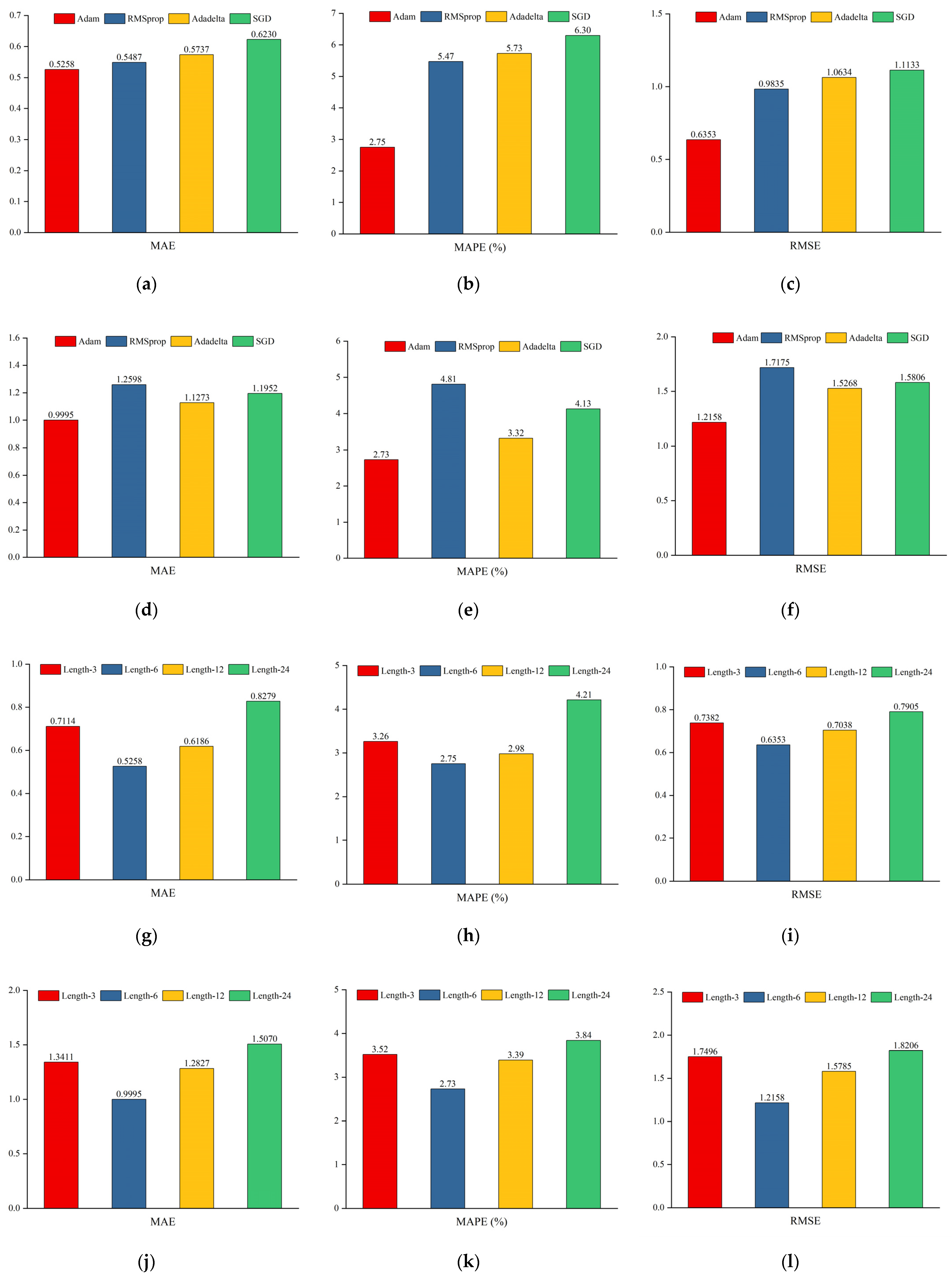
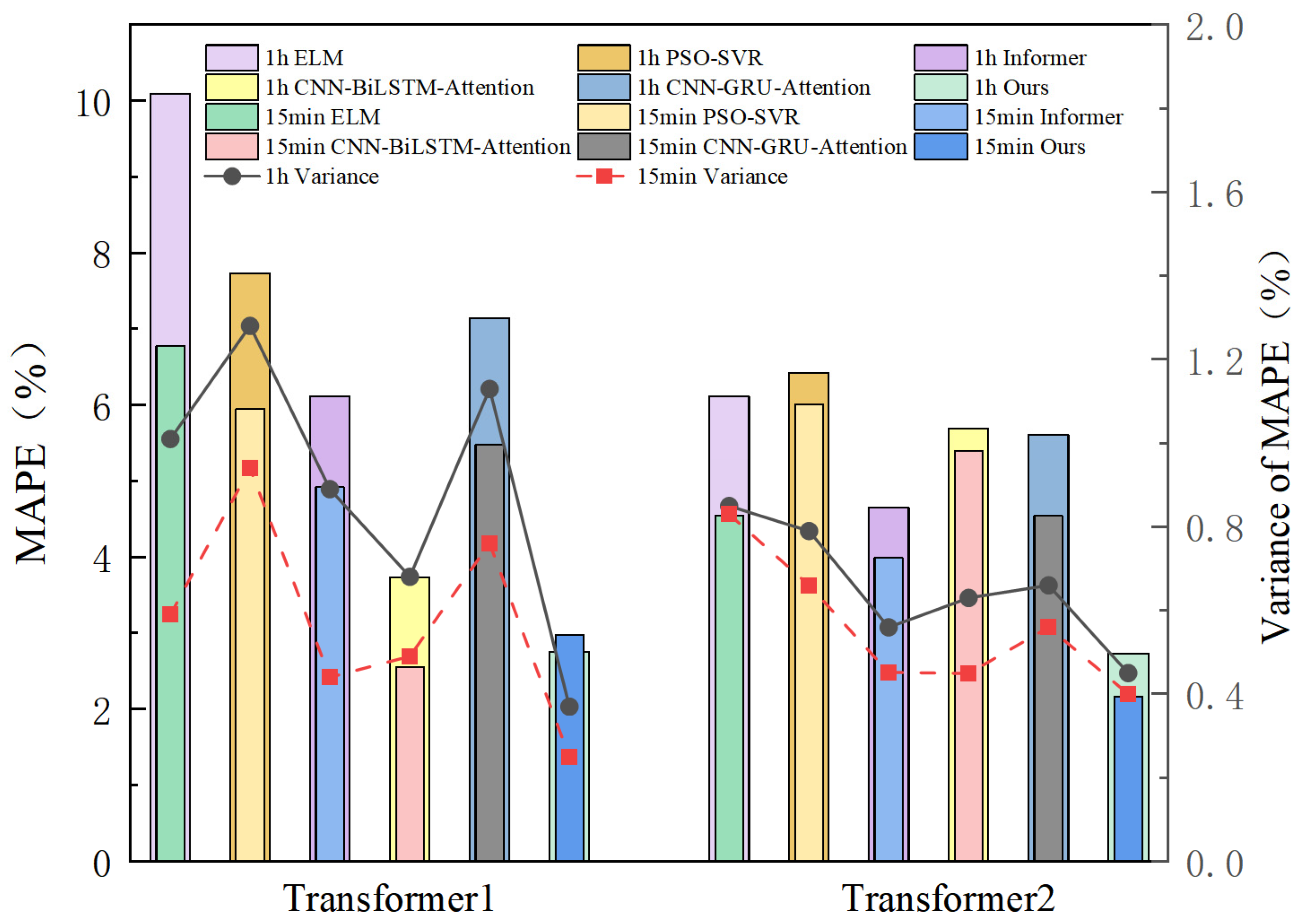
This study successfully developed and validated a novel BWO-TCN-BiGRU-Attention model for predicting the top oil temperature of transformers. The model integrates the strengths of various advanced technologies, including BWO for hyperparameter optimization, TCN for capturing short-term dependencies, BiGRU for handling long-term dependencies, and the attention mechanism for enhancing feature extraction. The experimental results demonstrate that, on the Transformer 1 dataset, the model achieved an MAE of 0.5258, a MAPE of 2.75%, and an RMSE of 0.6353; on the Transformer 2 dataset, the MAE was 0.9995, the MAPE was 2.73%, and the RMSE was 1.2158. In seasonal tests, the model’s MAPE was 2.75% in spring, 3.44% in summer, 3.93% in autumn, and 2.46% in winter for Transformer 1, and 2.73%, 2.78%, 3.07%, and 2.05% for Transformer 2, respectively, outperforming the benchmark models. Across the different time granularities, the model exhibited strong generalization ability and stability. At a time granularity of 1 h, the MAPE for Transformer 1 was 2.75% and for Transformer 2 was 2.73%. At a 15 min time granularity, the MAPE for Transformer 1 slightly increased to 2.98%, with a marginal rise in error but still maintaining the best performance; the MAPE for Transformer 2 further decreased to 2.16%. The BWO algorithm applied in this study has certain limitations. It may require significant computational resources in high-dimensional spaces and necessitates parameter tuning to maintain stable performance across tasks. Additionally, geographical diversity and transformer types may potentially impact the model’s generalizability. To ascertain the model’s adaptability, future research should conduct tests across a broader range of geographical areas and various types of transformers. Additionally, investigations should explore the architecture’s applicability to other power systems and climates, and examine the feasibility of deploying this algorithm for real-time predictive models. Furthermore, we intend to incorporate multi-source data, including environmental temperature, humidity, and transformer service life, to enrich input features and enhance predictive accuracy. These endeavors aim to provide robust technical support for the stable operation of smart grids and related fields.

References

- Liu, X.; Xie, J.; Luo, Y.; Yang, D. A Novel Power Transformer Fault Diagnosis Method Based on Data Augmentation for KPCA and Deep Residual Network. Energy Rep. 2023, 9, 620–627. [Google Scholar] [CrossRef]
- Xu, J.; Hao, J.; Zhang, N.; Liao, R.; Feng, Y.; Liao, W.; Cheng, H. Simulation Study on Converter Transformer Windings Stress Characteristics under Harmonic Current and Temperature Rise Effect. Int. J. Electr. Power Energy Syst. 2025, 165, 110505. [Google Scholar] [CrossRef]
- Olivares-Galván, J.C.; Georgilakis, P.S.; Ocon-Valdez, R. A Review of Transformer Losses. Electr. Power Compon. Syst. 2009, 37, 1046–1062. [Google Scholar] [CrossRef]
- Tsili, M.A.; Amoiralis, E.I.; Kladas, A.G.; Souflaris, A.T. Power Transformer Thermal Analysis by Using an Advanced Coupled 3D Heat Transfer and Fluid Flow FEM Model. Int. J. Therm. Sci. 2012, 53, 188–201. [Google Scholar] [CrossRef]
- Sun, L.; Xu, M.; Ren, H.; Hu, S.; Feng, G. Multi-Point Grounding Fault Diagnosis and Temperature Field Coupling Analysis of Oil-Immersed Transformer Core Based on Finite Element Simulation. Case Stud. Therm. Eng. 2024, 55, 104108. [Google Scholar] [CrossRef]
- Guo, Y.; Chang, Y.; Lu, B. A Review of Temperature Prediction Methods for Oil-Immersed Transformers. Measurement 2025, 239, 115383. [Google Scholar] [CrossRef]
- Singh, J.; Singh, S.; Singh, A. Distribution Transformer Failure Modes, Effects and Criticality Analysis (FMECA). Eng. Fail. Anal. 2019, 99, 180–191. [Google Scholar] [CrossRef]
- Zhao, Z.; Xu, J.; Zang, Y.; Hu, R. Adaptive Abnormal Oil Temperature Diagnosis Method of Transformer Based on Concept Drift. Appl. Sci. 2021, 11, 6322. [Google Scholar] [CrossRef]
- Fauzi, N.A.; Ali, N.H.N.; Ker, P.J.; Thiviyanathan, V.A.; Leong, Y.S.; Sabry, A.H.; Jamaludin, Z.B.; Lo, C.K.; Mun, L.H. Fault Prediction for Power Transformer Using Optical Spectrum of Transformer Oil and Data Mining Analysis. IEEE Access 2020, 8, 136374–136381. [Google Scholar] [CrossRef]
- Beheshti Asl, M.; Fofana, I.; Meghnefi, F. Review of Various Sensor Technologies in Monitoring the Condition of Power Transformers. Energies 2024, 17, 3533. [Google Scholar] [CrossRef]
- Zhu, J.; Xu, Y.; Peng, C.; Zhao, S. Fault Analysis of Oil-Immersed Transformer Based on Digital Twin Technology. J. Comput. Electron. Inf. Manag. 2024, 14, 9–15. [Google Scholar] [CrossRef]
- Zhang, P.; Zhang, Q.; Hu, H.; Hu, H.; Peng, R.; Liu, J. Research on Transformer Temperature Early Warning Method Based on Adaptive Sliding Window and Stacking. Electronics 2025, 14, 373. [Google Scholar] [CrossRef]
- Yang, L.; Chen, L.; Zhang, F.; Ma, S.; Zhang, Y.; Yang, S. A Transformer Oil Temperature Prediction Method Based on Data-Driven and Multi-Model Fusion. Processes 2025, 13, 302. [Google Scholar] [CrossRef]
- Zheng, H.; Li, X.; Feng, Y.; Yang, H.; Lv, W. Investigation on Micro-mechanism of Palm Oil as Natural Ester Insulating Oil for Overheating Thermal Fault Analysis of Transformers. High Volt. 2022, 7, 812–824. [Google Scholar] [CrossRef]
- Vatsa, A.; Hati, A.S.; Rathore, A.K. Enhancing Transformer Health Monitoring With AI-Driven Prognostic Diagnosis Trends: Overcoming Traditional Methodology’s Computational Limitations. IEEE Ind. Electron. Mag. 2024, 18, 30–44. [Google Scholar] [CrossRef]
- Meshkatodd, M.R. Aging Study and Lifetime Estimation of Transformer Mineral Oil. Am. J. Eng. Appl. Sci. 2008, 1, 384–388. [Google Scholar] [CrossRef]
- Abdali, A.; Abedi, A.; Mazlumi, K.; Rabiee, A.; Guerrero, J.M. Novel Hotspot Temperature Prediction of Oil-Immersed Distribution Transformers: An Experimental Case Study. IEEE Trans. Ind. Electron. 2023, 70, 7310–7322. [Google Scholar] [CrossRef]
- Nordman, H.; Lahtinen, M. Thermal Overload Tests on a 400-MVA Power Transformer with a Special 2.5-p.u. Short Time Loading Capability. IEEE Trans. Power Deliv. 2003, 18, 107–112. [Google Scholar] [CrossRef]
- Thiviyanathan, V.A.; Ker, P.J.; Leong, Y.S.; Abdullah, F.; Ismail, A.; Jamaludin, Z. Power Transformer Insulation System: A Review on the Reactions, Fault Detection, Challenges and Future Prospects. Alex. Eng. J. 2022, 61, 7697–7713. [Google Scholar] [CrossRef]
- Hamed Samimi, M.; Dadashi Ilkhechi, H. Survey of Different Sensors Employed for the Power Transformer Monitoring. IET Sci. Meas. Amp. Technol. 2020, 14, 1–8. [Google Scholar] [CrossRef]
- Na, Q.; Wen, Y. Design of Multi-Point Intelligent Temperature Monitoring System for Transformer Equipment. J. Phys. Conf. Ser. 2020, 1550, 062007. [Google Scholar] [CrossRef]
- Wang, Y.; Zhao, D.; Jia, Y.; Wang, S.; Du, Y.; Li, H.; Zhang, B. Acoustic Sensors for Monitoring and Localizing Partial Discharge Signals in Oil-Immersed Transformers under Array Configuration. Sensors 2024, 24, 4704. [Google Scholar] [CrossRef] [PubMed]
- Amoda, O.A.; Tylavsky, D.J.; McCulla, G.A.; Knuth, W.A. Acceptability of Three Transformer Hottest-Spot Temperature Models. IEEE Trans. Power Deliv. 2012, 27, 13–22. [Google Scholar] [CrossRef]
- Sippola, M.; Sepponen, R.E. Accurate Prediction of High-Frequency Power-Transformer Losses and Temperature Rise. IEEE Trans. Power Electron. 2002, 17, 835–847. [Google Scholar] [CrossRef]
- Deng, Y.; Ruan, J.; Quan, Y.; Gong, R.; Huang, D.; Duan, C.; Xie, Y. A Method for Hot Spot Temperature Prediction of a 10 kV Oil-Immersed Transformer. IEEE Access 2019, 7, 107380–107388. [Google Scholar] [CrossRef]
- Lyu, Z.; Wan, Z.; Bian, Z.; Liu, Y.; Zhao, W. Integrated Digital Twins System for Oil Temperature Prediction of Power Transformer Based On Internet of Things. IEEE Internet Things J. 2025, 2025, 3530440. [Google Scholar] [CrossRef]
- Institute of Electrical and Electronics Engineers. IEEE Guide for Loading Mineral-Oil-Immersed Transformers and Step-Voltage Regulators; Institute of Electrical and Electronics Engineers, IEEE-SA Standards Board, Eds.; Institute of Electrical and Electronics Engineers: New York, NY, USA, 2012; ISBN 9780738171951. [Google Scholar]
- Hippert, H.S.; Pedreira, C.E.; Souza, R.C. Neural Networks for Short-Term Load Forecasting: A Review and Evaluation. IEEE Trans. Power Syst. 2001, 16, 44–55. [Google Scholar] [CrossRef]
- Taheri, A.A.; Abdali, A.; Rabiee, A. A Novel Model for Thermal Behavior Prediction of Oil-Immersed Distribution Transformers With Consideration of Solar Radiation. IEEE Trans. Power Deliv. 2019, 34, 1634–1646. [Google Scholar] [CrossRef]
- Cheng, L.; Yu, T. Dissolved Gas Analysis Principle-Based Intelligent Approaches to Fault Diagnosis and Decision Making for Large Oil-Immersed Power Transformers: A Survey. Energies 2018, 11, 913. [Google Scholar] [CrossRef]
- Rao, W.; Zhu, L.; Pan, S.; Yang, P.; Qiao, J. Bayesian Network and Association Rules-Based Transformer Oil Temperature Prediction. J. Phys. Conf. Ser. 2019, 1314, 012066. [Google Scholar] [CrossRef]
- Zhang, X.; Liu, G.; Wang, H.; Li, X. Application of a Hybrid Interpolation Method Based on Support Vector Machine in the Precipitation Spatial Interpolation of Basins. Water 2017, 9, 760. [Google Scholar] [CrossRef]
- Lee, K.-R. A Study on SVM-Based Speaker Classification Using GMM-Supervector. J. IKEEE 2020, 24, 1022–1027. [Google Scholar] [CrossRef]
- Smyl, S. A Hybrid Method of Exponential Smoothing and Recurrent Neural Networks for Time Series Forecasting. Int. J. Forecast. 2020, 36, 75–85. [Google Scholar] [CrossRef]
- Xi, Y.; Lin, D.; Yu, L.; Chen, B.; Jiang, W.; Chen, G. Oil Temperature Prediction of Power Transformers Based on Modified Support Vector Regression Machine. Int. J. Emerg. Electr. Power Syst. 2023, 24, 367–375. [Google Scholar] [CrossRef]
- Huang, S.-J.; Shih, K.-R. Short-Term Load Forecasting via ARMA Model Identification Including Non-Gaussian Process Considerations. IEEE Trans. Power Syst. 2003, 18, 673–679. [Google Scholar] [CrossRef]
- Zhang, T.; Sun, H.; Peng, F.; Zhao, S.; Yan, R. A Deep Transfer Regression Method Based on Seed Replacement Considering Balanced Domain Adaptation. Eng. Appl. Artif. Intell. 2022, 115, 105238. [Google Scholar] [CrossRef]
- Cuk, A.; Bezdan, T.; Jovanovic, L.; Antonijevic, M.; Stankovic, M.; Simic, V.; Zivkovic, M.; Bacanin, N. Tuning Attention Based Long-Short Term Memory Neural Networks for Parkinson’s Disease Detection Using Modified Metaheuristics. Sci. Rep. 2024, 14, 4309. [Google Scholar] [CrossRef]
- Jovanovic, A.; Jovanovic, L.; Zivkovic, M.; Bacanin, N.; Simic, V.; Pamucar, D.; Antonijevic, M. Particle Swarm Optimization Tuned Multi-Headed Long Short-Term Memory Networks Approach for Fuel Prices Forecasting. J. Netw. Comput. Appl. 2025, 233, 104048. [Google Scholar] [CrossRef]
- Lin, J.; Van Wijngaarden, A.J.D.L.; Wang, K.-C.; Smith, M.C. Speech Enhancement Using Multi-Stage Self-Attentive Temporal Convolutional Networks. IEEE/ACM Trans. Audio Speech Lang. Process. 2021, 29, 3440–3450. [Google Scholar] [CrossRef]
- Fernando, T.; Sridharan, S.; Denman, S.; Ghaemmaghami, H.; Fookes, C. Robust and Interpretable Temporal Convolution Network for Event Detection in Lung Sound Recordings. IEEE J. Biomed. Health Inform. 2022, 26, 2898–2908. [Google Scholar] [CrossRef]
- Yang, Z.; Liao, W.; Liu, K.; Chen, X.; Zhu, R. Power Quality Disturbances Classification Using A TCN-CNN Model. In Proceedings of the 2022 7th Asia Conference on Power and Electrical Engineering (ACPEE), Hangzhou, China, 16–17 April 2022; IEEE: Piscataway, NJ, USA, 2022; pp. 2145–2149. [Google Scholar]
- Wang, X.; Xie, G.; Zhang, Y.; Liu, H.; Zhou, L.; Liu, W.; Gao, Y. The Application of a BiGRU Model with Transformer-Based Error Correction in Deformation Prediction for Bridge SHM. Buildings 2025, 15, 542. [Google Scholar] [CrossRef]
- Sun, R.; Chen, J.; Li, B.; Piao, C. State of Health Estimation for Lithium-Ion Batteries Based on Novel Feature Extraction and BiGRU-Attention Model. Energy 2025, 319, 134756. [Google Scholar] [CrossRef]
- Zhang, X.; Zhao, H.; Yao, J.; Wang, Z.; Zheng, Y.; Peng, T.; Zhang, C. A Multi-Scale Component Feature Learning Framework Based on CNN-BiGRU and Online Sequential Regularized Extreme Learning Machine for Wind Speed Prediction. Renew. Energy 2025, 242, 122427. [Google Scholar] [CrossRef]
- Dong, Y.; Zhong, Z.; Zhang, Y.; Zhu, R.; Wen, H.; Han, R. Intelligent Prediction Method of Hot Spot Temperature in Transformer by Using CNN-LSTM&GRU Network. In Proceedings of the 2023 International Conference on Advanced Robotics and Mechatronics (ICARM), Sanya, China, 8 July 2023; IEEE: Piscataway, NJ, USA, 2023; pp. 7–12. [Google Scholar]
- Wang, X.; Liu, X.; Bai, Y. Prediction of the Temperature of Diesel Engine Oil in Railroad Locomotives Using Compressed Information-Based Data Fusion Method with Attention-Enhanced CNN-LSTM. Appl. Energy 2024, 367, 123357. [Google Scholar] [CrossRef]
- Zou, D.; Xu, H.; Quan, H.; Yin, J.; Peng, Q.; Wang, S.; Dai, W.; Hong, Z. Top-Oil Temperature Prediction of Power Transformer Based on Long Short-Term Memory Neural Network with Self-Attention Mechanism Optimized by Improved Whale Optimization Algorithm. Symmetry 2024, 16, 1382. [Google Scholar] [CrossRef]
- Abualigah, L. Particle Swarm Optimization: Advances, Applications, and Experimental Insights. Comput. Mater. Contin. 2025, 82, 1539–1592. [Google Scholar] [CrossRef]
- Ballerini, L. Particle Swarm Optimization in 3D Medical Image Registration: A Systematic Review. Arch. Comput. Methods Eng. 2025, 32, 311–318. [Google Scholar] [CrossRef]
- Ma, J.; Gao, W.; Tong, W. A Deep Reinforcement Learning Assisted Adaptive Genetic Algorithm for Flexible Job Shop Scheduling. Eng. Appl. Artif. Intell. 2025, 149, 110447. [Google Scholar] [CrossRef]
- Chen, Y.; Dong, Z.; Wang, Y.; Su, J.; Han, Z.; Zhou, D.; Zhang, K.; Zhao, Y.; Bao, Y. Short-Term Wind Speed Predicting Framework Based on EEMD-GA-LSTM Method under Large Scaled Wind History. Energy Convers. Manag. 2021, 227, 113559. [Google Scholar] [CrossRef]
- Emary, E.; Zawbaa, H.M.; Grosan, C. Experienced Gray Wolf Optimization Through Reinforcement Learning and Neural Networks. IEEE Trans. Neural Netw. Learn. Syst. 2018, 29, 681–694. [Google Scholar] [CrossRef]
- Yang, Y.; Yan, J.; Zhou, X. A Heat Load Prediction Method for District Heating Systems Based on the AE-GWO-GRU Model. Appl. Sci. 2024, 14, 5446. [Google Scholar] [CrossRef]
- Yue, Y.; Cao, L.; Lu, D.; Hu, Z.; Xu, M.; Wang, S.; Li, B.; Ding, H. Review and Empirical Analysis of Sparrow Search Algorithm. Artif. Intell. Rev. 2023, 56, 10867–10919. [Google Scholar] [CrossRef]
- Mohammed, H.M.; Umar, S.U.; Rashid, T.A. A Systematic and Meta-Analysis Survey of Whale Optimization Algorithm. Comput. Intell. Neurosci. 2019, 2019, 8718571. [Google Scholar] [CrossRef] [PubMed]
- Zhu, D.; Li, R.; Zheng, Y.; Zhou, C.; Li, T.; Cheng, S. Cumulative Major Advances in Particle Swarm Optimization from 2018 to the Present: Variants, Analysis and Applications. Arch. Comput. Methods Eng. 2025, 32, 1571–1595. [Google Scholar] [CrossRef]
- Dehghani, M.; Hubalovsky, S.; Trojovsky, P. Northern Goshawk Optimization: A New Swarm-Based Algorithm for Solving Optimization Problems. IEEE Access 2021, 9, 162059–162080. [Google Scholar] [CrossRef]
- Li, Y.; Lin, X.; Liu, J. An Improved Gray Wolf Optimization Algorithm to Solve Engineering Problems. Sustainability 2021, 13, 3208. [Google Scholar] [CrossRef]
- Mirjalili, S.; Lewis, A. The Whale Optimization Algorithm. Adv. Eng. Softw. 2016, 95, 51–67. [Google Scholar] [CrossRef]
- Heidari, A.A.; Mirjalili, S.; Faris, H.; Aljarah, I.; Mafarja, M.; Chen, H. Harris Hawks Optimization: Algorithm and Applications. Future Gener. Comput. Syst. 2019, 97, 849–872. [Google Scholar] [CrossRef]
- Dorigo, M.; Birattari, M.; Stutzle, T. Ant Colony Optimization. IEEE Comput. Intell. Mag. 2006, 1, 28–39. [Google Scholar] [CrossRef]
- Dehghani, M.; Montazeri, Z.; Trojovská, E.; Trojovský, P. Coati Optimization Algorithm: A New Bio-Inspired Metaheuristic Algorithm for Solving Optimization Problems. Knowl. Based Syst. 2023, 259, 110011. [Google Scholar] [CrossRef]
- Gharehchopogh, F.S.; Namazi, M.; Ebrahimi, L.; Abdollahzadeh, B. Advances in Sparrow Search Algorithm: A Comprehensive Survey. Arch. Comput. Methods Eng. 2023, 30, 427–455. [Google Scholar] [CrossRef] [PubMed]
- Van Laarhoven, P.J.M.; Aarts, E.H.L. Simulated Annealing: Theory and Applications; Springer: Dordrecht, The Netherlands, 1987; ISBN 9789048184385. [Google Scholar]
- Karaboğa, D.; Ökdem, S. A Simple and Global Optimization Algorithm for Engineering Problems: Differential Evolution Algorithm. Turk. J. Electr. Eng. Comput. Sci. 2004, 12, 53–60. [Google Scholar]
- Mitchell, M. An Introduction to Genetic Algorithms; Complex Adaptive Systems, 7 Print; The MIT Press: Cambridge, MA, USA, 2001; ISBN 9780262631853. [Google Scholar]
- Zhong, C.; Li, G.; Meng, Z. Beluga Whale Optimization: A Novel Nature-Inspired Metaheuristic Algorithm. Knowl. Based Syst. 2022, 251, 109215. [Google Scholar] [CrossRef]
- Wan, A.; Peng, S.; AL-Bukhaiti, K.; Ji, Y.; Ma, S.; Yao, F.; Ao, L. A Novel Hybrid BWO-BiLSTM-ATT Framework for Accurate Offshore Wind Power Prediction. Ocean. Eng. 2024, 312, 119227. [Google Scholar] [CrossRef]
- Wolpert, D.H.; Macready, W.G. No free lunch theorems for optimization. IEEE Trans. Evol. Computat. 1997, 1, 67–82. [Google Scholar] [CrossRef]
- Lara-Benítez, P.; Carranza-García, M.; Luna-Romera, J.M.; Riquelme, J.C. Temporal Convolutional Networks Applied to Energy-Related Time Series Forecasting. Appl. Sci. 2020, 10, 2322. [Google Scholar] [CrossRef]
- Feng, Y.; Zhu, J.; Qiu, P.; Zhang, X.; Shuai, C. Short-Term Power Load Forecasting Based on TCN-BiLSTM-Attention and Multi-Feature Fusion. Arab. J. Sci. Eng. 2024, 50, 5475–5486. [Google Scholar] [CrossRef]
- Li, X.; Zhou, S.; Wang, F. A CNN-BiGRU Sea Level Height Prediction Model Combined with Bayesian Optimization Algorithm. Ocean. Eng. 2025, 315, 119849. [Google Scholar] [CrossRef]
- Ławryńczuk, M.; Zarzycki, K. LSTM and GRU Type Recurrent Neural Networks in Model Predictive Control: A Review. Neurocomputing 2025, 632, 129712. [Google Scholar] [CrossRef]
- Karthik, R.V.; Pandiyaraju, V.; Ganapathy, S. A Context and Sequence-Based Recommendation Framework Using GRU Networks. Artif. Intell. Rev. 2025, 58, 170. [Google Scholar] [CrossRef]
- Teng, F.; Song, Y.; Guo, X. Attention-TCN-BiGRU: An Air Target Combat Intention Recognition Model. Mathematics 2021, 9, 2412. [Google Scholar] [CrossRef]
- Niu, Z.; Zhong, G.; Yu, H. A Review on the Attention Mechanism of Deep Learning. Neurocomputing 2021, 452, 48–62. [Google Scholar] [CrossRef]
- Hernández, A.; Amigó, J.M. Attention Mechanisms and Their Applications to Complex Systems. Entropy 2021, 23, 283. [Google Scholar] [CrossRef] [PubMed]
- Zhou, H.; Zhang, S.; Peng, J.; Zhang, S.; Li, J.; Xiong, H.; Zhang, W. Informer: Beyond Efficient Transformer for Long Sequence Time-Series Forecasting. Proc. AAAI Conf. Artif. Intell. 2021, 35, 11106–11115. [Google Scholar] [CrossRef]
- Xue, J.; Shen, B. Dung Beetle Optimizer: A New Meta-Heuristic Algorithm for Global Optimization. J. Supercomput. 2023, 79, 7305–7336. [Google Scholar] [CrossRef]
- Kennedy, J.; Eberhart, R. Particle swarm optimization. In Proceedings of the ICNN’95—International Conference on Neural Networks, Perth, WA, Australia, 27 November–1 December 1995; IEEE: Piscataway, NJ, USA, 1995; pp. 1942–1948. [Google Scholar] [CrossRef]
- Sumida, B.H.; Houston, A.I.; McNamara, J.M.; Hamilton, W.D. Genetic algorithms and evolution. J. Theor. Biol. 1990, 147, 59–84. [Google Scholar] [CrossRef]
- Watanabe, O.; Zeugmann, T. (Eds.) Stochastic Algorithms: Foundations and Applications; Springer: Berlin/Heidelberg, Germany, 2009. [Google Scholar] [CrossRef]
- Shiyong, L.; Jing, X.; Mianzhi, W.; Rongbin, X.; Bin, J.; Kai, W.; Qingquan, L. Prediction of Transformer Top Oil Temperature Based on Improved Weighted Support Vector Regression Based on Particle Swarm Optimization. In Proceedings of the 2021 International Conference on Advanced Electrical Equipment and Reliable Operation (AEERO), Beijing, China, 15–17 October 2021; IEEE: Piscataway, NJ, USA, 2021; pp. 1–5. [Google Scholar]
Disclaimer/Publisher’s Note: The statements, opinions and data contained in all publications are solely those of the individual author(s) and contributor(s) and not of MDPI and/or the editor(s). MDPI and/or the editor(s) disclaim responsibility for any injury to people or property resulting from any ideas, methods, instructions or products referred to in the content. |
© 2025 by the authors. Licensee MDPI, Basel, Switzerland. This article is an open access article distributed under the terms and conditions of the Creative Commons Attribution (CC BY) license (https://creativecommons.org/licenses/by/4.0/).