A Hybrid Evolutionary Fuzzy Ensemble Approach for Accurate Software Defect Prediction

Abstract

Software defect prediction identifies defect-prone modules before testing, reducing costs and development time. Machine learning techniques are widely used, but high-dimensional datasets often degrade classification accuracy due to irrelevant features. To address this, effective feature selection is essential but remains an NP-hard challenge best tackled with heuristic algorithms. This study introduces a binary, multi-objective starfish optimizer for optimal feature selection, balancing feature reduction and classification performance. A Choquet fuzzy integral-based ensemble classifier further enhances prediction reliability by aggregating multiple classifiers. The approach was validated on five NASA datasets, demonstrating superior performance over traditional classifiers. Key software metrics—such as design complexity, operators and operands count, lines of code, and numbers of branches—were found to significantly influence defect prediction. The results show that the proposed method improves classification performance by 1% to 13% while retaining only 33% to 57% of the original feature set, offering a reliable and interpretable solution for software defect prediction. This approach holds strong potential for broader, high-dimensional classification tasks.

1. Introduction

The presence of defects in software systems poses a significant challenge in modern software engineering, affecting software reliability, maintainability, and security. Software defects can lead to system failures, performance degradation, and increased operational costs, making their early detection a critical aspect of software quality assurance. As software complexity increases, the need for effective software defect prediction (SDP) becomes more pressing. SDP aims to identify defect-prone software modules before testing and deployment, allowing developers to focus their efforts on these areas, thereby optimizing resource allocation and improving software quality [1,2,3].

Traditional defect detection methods, such as manual code reviews and testing, are often time-consuming, expensive, and prone to human error, especially in large-scale software projects [4]. Consequently, automated defect prediction techniques have gained significant attention, particularly those leveraging machine learning (ML) models. However, despite the promising results achieved by ML-based approaches, several challenges remain unresolved.

One of the major challenges in software defect prediction is the high dimensionality of defect datasets. This results in excessive software metrics, such as lines of code, complexity measures, and structural properties, which introduce redundant information and noise, ultimately reducing classification accuracy [5,6]. Feature selection plays a key role in mitigating this problem by eliminating irrelevant and redundant features and thereby improving classification accuracy and generalizability. However, feature selection is an NP-hard problem, making exhaustive search methods impractical for large-scale datasets. To address this, evolutionary optimization algorithms have emerged as a promising solution, effectively identifying the most informative features for software defect prediction while reducing computational overhead.

Additionally, current SDP methods are often limited because they depend on single classifiers, which can become unstable and overfit when trained on uneven defect datasets. Ensemble learning addresses this limitation by combining multiple classifiers to improve predictive performance. Traditional ensemble techniques, on the other hand, rely on simple aggregation methods, like majority voting or averaging, that do not consider interactions among classifiers [7,8,9]. These conditions can lead to suboptimal prediction accuracy, especially when classifiers exhibit correlated errors. Consequently, there is a need for advanced aggregation methods that can optimally fuse the outputs of multiple classifiers while considering their interdependencies.

To address these challenges, this study proposes a novel hybrid evolutionary fuzzy ensemble approach for software defect prediction. The proposed framework integrates two key components:

• Binary Multi-Objective Starfish Optimizer (Bmosfo) for Feature Selection:A binary, multi-objective version of the starfish optimizer (BMOSFO) is introduced for feature selection, ensuring that only the most relevant software metrics are considered, improving classification performance. BMOSFO leverages the unique behaviors of starfish, such as regeneration and multidimensional movement, to balance exploration and exploitation in high-dimensional feature spaces. This enables the effective navigation of complex feature subsets, achieving superior convergence speed and computational efficiency compared to conventional evolutionary algorithms.
• Choquet Fuzzy Integral-based Ensemble Classification: To enhance classification accuracy, a Choquet fuzzy integral-based ensemble classifier was developed. Unlike traditional ensemble methods that assume classifier independence, the Choquet integral considers interactions among classifiers, enabling more informed decision fusion. By optimally aggregating multiple machine learning models, including k-nearest neighbors (KNNs) [10], support vector machines (SVMs) [11,12], decision trees (DTs) [13], logistic regression (LR) [14], random forest (RF) [15,16], gaussian naïve Bayes (GNB) [17,18], and artificial neural networks (ANNs) [19,20,21], the Choquet integral enhances defect prediction reliability by accounting for the interdependencies among classifiers.

The key contributions of this study are as follows:

• Introduction of BMOSFO for Feature Selection: BMOSFO is designed to efficiently reduce feature dimensionality while maintaining high classification accuracy. It achieves this by balancing exploration and exploitation through unidimensional and five-dimensional search mechanisms, inspired by starfish regeneration and movement behaviors.
• Development of a Choquet Fuzzy Integral-based Ensemble Classifier: A novel ensemble method is introduced to optimally aggregate multiple ML models, leveraging the Choquet integral’s ability to consider interdependencies among classifiers, thereby enhancing predictive accuracy and robustness [22].
• Comprehensive Evaluation on Real-World Datasets: The proposed approach is rigorously evaluated on five real-world benchmark datasets, demonstrating superior performance compared to traditional feature selection and classification methods.
• Insightful Feature Impact Analysis: An in-depth analysis of the most impactful software metrics, including design complexity, number of operators and operands, development time, lines of code, commented lines, numbers of branches, and operand sums, is conducted to highlight their significance in defect prediction.

The proposed framework addresses the limitations of conventional defect prediction models by integrating evolutionary optimization and fuzzy ensemble learning, contributing to improved accuracy and interpretability in software defect classification. The approach not only enhances defect prediction performance but also provides actionable insights into the impact of key software metrics, facilitating more reliable software quality assurance practices.

The remainder of this paper is structured as follows. Section 2 presents a comprehensive review of related work on predictive modeling for software defect detection. Section 3 details the proposed methodology, including dataset descriptions, the starfish optimizer, the BMOSFO algorithm, and the functioning of the Choquet fuzzy integral-based ensemble classification. Section 4 describes the experimental setup, evaluation metrics, and benchmark techniques. Section 5 discusses the experimental findings, including an in-depth analysis of model performance and feature selection impact. Section 6 summarizes this study’s key findings, discusses limitations, and outlines potential future research directions in predictive modeling for software defect detection.

2. Related Work

This section provides an overview of related research in the area of software defect prediction, categorized into four primary approaches: (1) machine learning (ML)-based defect prediction, (2) deep learning (DL)-based approaches, (3) evolutionary algorithms, and (4) ensemble methods. Each category contributes to advancing defect prediction models by addressing challenges related to accuracy, feature selection, and model stability. This section critically analyzes key studies within these categories, highlighting their strengths, limitations, and the research gaps that motivated the proposed hybrid evolutionary fuzzy ensemble approach.

2.1. Machine Learning Approaches for Software Defect Prediction

Several studies have explored the use of machine learning models for software defect prediction. In [23], a tree-boosting algorithm (XGBoost) was employed to predict software defects using module features that are easily computable. A model sampling strategy was proposed to enhance explainability while maintaining predictive performance. A cloud-based architecture was developed in [24] to facilitate real-time software defect detection, incorporating four backpropagation training algorithms along with a fuzzy layer to optimize training function selection. The experimental results demonstrated the effectiveness of Bayesian regularization and scaled conjugate gradient methods in improving prediction accuracy.

Efforts have also been made to improve classification performance using hybrid approaches. A technique combining K-means clustering, classification models, and particle swarm optimization (PSO) was introduced in [25], demonstrating that the SVM and its enhanced variant achieved the highest accuracy. Similarly, a meta-heuristic feature selection model utilizing random forest (RF), SVM, and PSO was evaluated in [26], where it was shown that feature dimensionality could be reduced by 75.15% while maintaining high classification accuracy. The impact of kernel functions on SVM-based defect prediction was analyzed in [27], where results indicated that utilizing the top 40% of selected features led to significant improvements in classification efficacy.

Traditional ML models often suffer from high-dimensional input spaces that introduce noise and redundancy, affecting classifier performance. In [11], different feature selection methods, including filter-based, wrapper-based, and hybrid approaches, were analyzed to determine their impact on classifier accuracy. The results showed that hybrid methods combining filter and wrapper techniques yielded the most significant performance gains. Another work [12] explored multi-objective feature selection techniques, demonstrating that optimization-based feature selection could further improve classification robustness while reducing computation time.

Although ML models have shown promising results, their performance is often hindered by the high dimensionality and redundancy of software metrics. This highlights the need for effective feature selection techniques, motivating the development of advanced evolutionary algorithms, as explored in this study.

2.2. Deep Learning Approaches for Software Defect Prediction

Deep learning (DL) techniques have gained attention for their ability to extract complex feature representations from software repositories. A neural network-based framework was introduced in [28] to predict software defects, achieving an 8% increase in squared correlation coefficient and a 14% reduction in mean square error compared to previous methods. Challenges related to context complexity and data scarcity in DL-based defect prediction were discussed in [29], where self-supervised training and transformer-based architectures were suggested to enhance code comprehension and reduce labeled data dependency.

To improve software defect detection, a gated hierarchical long short-term memory (GH-LSTM) network was proposed in [30], leveraging hierarchical LSTM networks to extract semantic features from abstract syntax trees (ASTs). Similarly, a BERT-based semantic feature extraction method combined with bidirectional long short-term memory (BiLSTM) networks was explored in [31]. Data augmentation techniques were employed to enhance training, leading to superior performance across ten open-source projects. A meta-analysis of 102 peer-reviewed studies on deep learning-based defect prediction was conducted in [32], emphasizing the need for replication packages, diverse software artifacts, and data augmentation to improve generalizability.

Recent studies have further examined the applicability of pre-trained deep learning models for software defect detection. Transformer-based architectures, including BERT and CodeBERT, have been evaluated for their ability to extract meaningful representations of code artifacts. Another study [21] focused on the integration of graph neural networks (GNNs) with deep learning models, leveraging software dependency graphs to improve feature learning for defect prediction.

Despite their superior feature extraction capabilities, DL models are challenged by data scarcity and context complexity in defect prediction tasks. This study addresses these limitations by integrating DL with fuzzy ensemble methods to enhance generalization and robustness [33].

2.3. Evolutionary Algorithms for Software Defect Prediction

Evolutionary computation techniques have been widely applied to enhance software defect prediction. In [34], a hybrid method combining a genetic algorithm (GA), SVM, and PSO was implemented across 24 datasets, including NASA MDP and Java open-source repositories. The results showed improved classification performance on both small and large datasets. A supervised differential evolution-based approach (DEJIT) was introduced in [35] for just-in-time software defect prediction (JIT-SDP), leading to substantial improvements in effort-aware prediction.

Further advancements have focused on optimizing evolutionary search strategies. In [36], a hybrid model combining the sparrow search algorithm (SSA) with PSO (SSA-PSO) was designed to accelerate convergence and improve classification accuracy. The Genetic Evolution (GeEv) framework was introduced in [37] to enhance feature selection diversity by evolving random offspring with higher survival potential. Similarly, a novel, three-parent genetic evolution method (3PcGE) was proposed in [38], demonstrating superior classification performance compared to conventional wrapper- and filter-based feature selection methods.

Recent studies have explored advanced optimization techniques to enhance the efficiency of software defect prediction models. One such approach introduced an improved reptile search algorithm (RSA) for hyperparameter tuning [39]. The experimental results on benchmark defect datasets demonstrated that RSA achieved superior classification accuracy compared to traditional swarm intelligence techniques, highlighting its potential for optimizing model parameters.

Another recent study [40] focused on optimizing individual classifiers before integrating them into an ensemble model. The approach involved the separate optimization of RF, SVM, and naïve Bayes classifiers, which were then combined using a voting ensemble strategy. This technique significantly enhanced computational efficiency, reducing training and testing times by 51.52% and 52.31%, respectively, while maintaining high classification accuracy. These findings reinforce the effectiveness of hybrid optimization and ensemble learning in improving defect prediction models.

Recently, hybrid evolutionary approaches were explored to optimize defect prediction models further. In [22], a parametric evolutionary technique was applied to dynamically adjust hyperparameters in defect prediction models. The study highlighted the advantages of adaptive evolutionary strategies over static parameter tuning, demonstrating improved model generalization and efficiency.

While existing evolutionary algorithms improve feature selection, they often suffer from slow convergence and premature stagnation. This motivates the introduction of BMOSFO, which leverages multidimensional search strategies inspired by starfish regeneration to enhance convergence speed and exploration capabilities.

2.4. Ensemble Approaches for Software Defect Prediction

Ensemble learning has been widely adopted in software defect prediction due to its ability to enhance classification accuracy by combining multiple models. Bagging, boosting, and stacking have been shown to mitigate overfitting while improving prediction robustness [41,42,43]. In [44], an ensemble multiple kernel correlation alignment (EMKCA) method was introduced for heterogeneous defect prediction. The approach applied kernel classifiers to transform the data distribution and address class imbalance, outperforming benchmark methods across 30 datasets.

A comparative evaluation of deep learning and machine learning models for defect classification was conducted in [45], where ensemble techniques, including bagging, boosting, and stacking, achieved superior predictive performance compared to standalone classifiers. In [46], a two-stage ensemble model was developed, integrating random forest (RF), support vector machines (SVMs), gaussian naïve Bayes (GNB), and artificial neural networks (ANNs) with final predictions determined using a voting ensemble. Similarly, a hybrid SMOTE–ensemble method was introduced in [47], employing bagging, RF, and AdaBoost to enhance classification performance in imbalanced datasets.

Additional advancements in ensemble learning include the use of principal component analysis (PCA) for feature selection, as demonstrated in [48]. A framework integrating PCA with ensemble classifiers showed that bagging achieved the highest classification accuracy of 91.49%, with feature reduction leading to an additional 0.6% increase in performance. An ensemble learning strategy combining KNN, RF, and ANNs was proposed in [49], demonstrating superior performance over individual classifiers.

Although ensemble learning enhances classification accuracy, traditional methods assume classifier independence, leading to suboptimal aggregation when classifiers exhibit correlated errors. The Choquet fuzzy integral addresses this by modeling interdependencies, enabling more informed decision fusion, as explored in this study.

In summary, while significant progress has been made in ML, DL, evolutionary, and ensemble approaches for software defect prediction, challenges related to feature selection, classifier interdependencies, and generalization remain unresolved. This study addresses these gaps by introducing a hybrid evolutionary fuzzy ensemble approach, leveraging BMOSFO for multi-objective feature selection and the Choquet fuzzy integral for advanced ensemble classification.

3. Proposed Hybrid Model for Software Defect Prediction

This section presents the proposed software defect prediction model, which integrates machine learning classifiers with binary, multi-objective starfish optimization (BMOSFO) for feature selection. The BMOSFO algorithm is employed to identify the most relevant software defect features, improving classification accuracy and computational efficiency. The machine learning models used in this study include artificial neural networks (ANNs), decision trees (DTs), random forest (RF), k-nearest neighbors (KNNs), naïve Bayes (NB), logistic regression (LR), and support vector machines (SVMs). Furthermore, an ensemble classifier based on the Choquet fuzzy integral is applied to aggregate predictions and enhance defect classification performance.

The integration of BMOSFO for feature selection with the Choquet fuzzy integral-based ensemble classification presents a novel approach in software defect prediction. This combination leverages the exploration–exploitation balance of BMOSFO and the interdependency modeling capability of the Choquet integral, leading to improved classification accuracy and interpretability. This innovative hybridization addresses the limitations of traditional defect prediction models by simultaneously optimizing feature relevance and classifier interaction, making it a robust solution for complex software datasets.

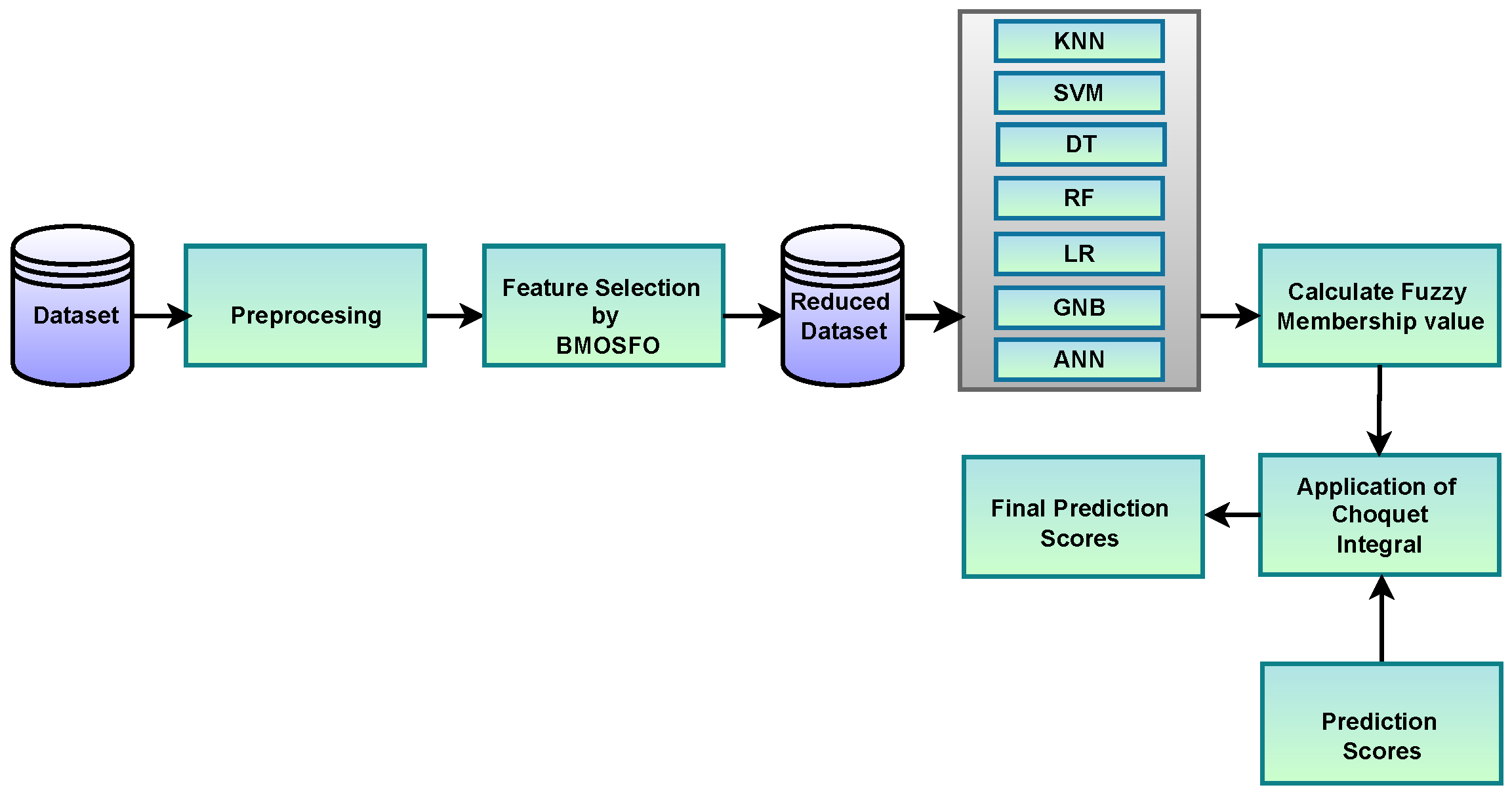
Figure 1 illustrates the workflow of the proposed software defect prediction framework.

The system follows a structured pipeline consisting of six key stages:

• Data Preprocessing: The input software defect datasets undergo normalization and preprocessing, where redundant and missing values are handled. This step ensures the quality of input features before optimization and classification.
• Feature Selection using BMOSFO: The binary, multi-objective starfish optimizer (BMOSFO) is applied to identify the most relevant defect prediction features. It optimizes two conflicting objectives: reducing the number of selected features while maximizing classification performance. BMOSFO integrates exploratory and exploitative search strategies to achieve an optimal balance, leading to more informative feature subsets.
• Training Multiple Machine Learning Classifiers: The selected features are used to train multiple machine learning models, including the KNN, SVM, DT, RF, NB, LR, and ANN. This diverse set of classifiers ensures robustness, leveraging different algorithmic paradigms to capture varying defect patterns.
• Computing Prediction Scores: Each trained classifier produces confidence scores for defect-prone modules, reflecting the likelihood of defects based on learned patterns from historical data. These scores indicate the likelihood of a software module being defective, contributing to the ensemble model’s decision-making process.
• Calculating Fuzzy Membership Values: Instead of simply aggregating classifier outputs, the Choquet fuzzy integral approach is applied. It calculates fuzzy membership values for each classifier, reflecting their influence in the ensemble and ensuring that classifiers with stronger predictive power have greater weight in the decision-making process.
• Aggregating Classifier Outputs using the Choquet Integral: The final prediction is determined using the Choquet fuzzy integral, which accounts for the interdependencies among classifiers rather than assuming that they are independent. This enhances prediction reliability by leveraging the strengths of different models while mitigating correlated errors.

Each feature in the dataset is represented as a binary feature vector in BMOSFO, as shown in Figure 2. If a feature’s associated bit is 1, it is retained in the training process; otherwise, it is removed. The BMOSFO algorithm optimizes feature selection by minimizing the number of selected features while ensuring high classification accuracy. The fitness function is designed to balance model simplicity and error minimization, progressively refining the selected feature set to reduce classification errors.

The datasets used in this study were obtained from the NASA repository [50], which has been publicly available since 2005. These datasets include software metrics such as branch count, Halstead’s complexity measures, McCabe’s cyclomatic complexity, and various line-of-code criteria.

Table 1. Description of NASA datasets.

Dataset	Programming Language	# of Modules	% of Defected Models	Description
JM1	C	13,204	16%	Software written in C, using Halstead and McCabe metrics for defect prediction.
KC1	C++	2109	15.4%	Storage management software handling ground data.
PC1	C	1109	6.8%	Flight software from an earth-orbiting satellite.
KC2	C++	522	20%	Science data processing software.
CM1	C	498	9.7%	NASA spacecraft instrument data processing.

summarizes the datasets, while

Table 2. Features present in NASA datasets.

SNO	Features
1	McCabe Metrics	Line count of code
2		Cyclomatic complexity
3		Essential complexity
4		Design complexity
5	Halstead Metrics	Total operators + operands
6		Volume
7		Program length
8		Difficulty
9		Intelligence
10		Effort
11		Number of delivered bugs
12		Time estimator
13		Line count
14		Count of lines of comments
15		Count of blank lines
16		Lines containing both code and comments
17	Unique operators
18	Unique operands
19	Total operators
20	Total operands
21	Branch count of the flow graph
22	Number of defects

provides an overview of the features used in this investigation.

The NASA datasets are particularly relevant for software defect prediction due to their high dimensionality, class imbalance, and noise levels, which present significant challenges for conventional machine learning models. These datasets contain complex software metrics such as cyclomatic complexity and Halstead measures, making them ideal for evaluating the effectiveness of the proposed BMOSFO feature selection and Choquet fuzzy integral-based ensemble classification. By testing the proposed model on these real-world datasets, this study demonstrates the robustness and generalizability of the approach in handling complex defect prediction scenarios.

The proposed model employs multi-objective optimization to balance feature selection efficiency and predictive accuracy. BMOSFO integrates swarm intelligence techniques with multi-objective search mechanisms to optimize the classifier’s performance. Inspired by starfish movement patterns, BMOSFO incorporates exploratory and exploitative search strategies, enabling the robust selection of relevant defect prediction features while minimizing computational overhead.

This section elaborates on the advantages of BMOSFO in software defect classification, detailing how binary optimization techniques enhance feature selection while maintaining model interpretability. Additionally, modifications for handling binary search spaces are introduced, ensuring compatibility with real-world software defect datasets.

3.1. Starfish Optimization Algorithm: Exploration and Exploitation Mechanisms

Feature selection is a fundamental step in software defect prediction as it aims to extract the most relevant attributes from high-dimensional datasets while maintaining predictive accuracy. However, this problem is inherently NP-hard, making exhaustive searches impractical for large datasets. As a result, heuristic-driven, stochastic search strategies, such as metaheuristic algorithms, have emerged as effective alternatives for efficiently navigating complex feature spaces.

A critical challenge in metaheuristic optimization is balancing exploration (global search capability) and exploitation (local refinement). A well-calibrated trade-off between these two phases is essential to avoid premature convergence to suboptimal solutions. Since metaheuristics rely on stochastic search mechanisms, they do not guarantee optimal solutions for every problem. The No-Free-Lunch (NFL) theorem [51] states that no single optimization algorithm consistently outperforms all others across all problem domains. Consequently, the development of problem-specific adaptive metaheuristics remains a key research focus.

While several recent metaheuristic algorithms, such as the crayfish optimization algorithm [52], the reptile search algorithm [53], and the red fox optimizer [54], have been introduced, this study pioneers the application of the starfish optimization algorithm (SFOA) [55] for feature selection. To the best of our knowledge, no existing study has investigated this framework for selecting informative defect prediction features. The proposed BMOSFO extends SFOA by incorporating a binary encoding scheme for feature selection and a multi-objective optimization strategy to maximize classification performance while minimizing feature subset size. BMOSFO draws inspiration from key biological characteristics of starfish, including regeneration, multi-directional movement, and adaptive hunting strategies, to achieve an optimal balance between exploration and exploitation.

Starfish, also known as sea stars, exhibit complex biological behaviors that serve as the foundation for BMOSFO. They comprise over 2000 species globally, most of which display a five-arm radial symmetry extending from a central disk. Some species possess more than five arms, with variations reaching ten or more [56]. Depending on environmental conditions and species characteristics, starfish can have lifespans ranging from ten to thirty-five years.

Figure 3 illustrates key starfish characteristics that influence BMOSFO’s optimization strategies. Figure 3a,b depict the body structure and multi-directional movement of different starfish species. BMOSFO mimics this behavior by implementing a multi-dimensional search mechanism that enhances global exploration. Figure 3c represents starfish regeneration, which serves as inspiration for BMOSFO’s dynamic feature refinement mechanism. This ability ensures that the search process continuously adapts to new promising solutions. Figure 3d illustrates prey interactions, which BMOSFO incorporates into its adaptive exploitation strategy to refine feature selection.

BMOSFO dynamically adjusts its search strategy based on the complexity of the feature space. Two primary search patterns are used:

• For high-dimensional feature spaces ($L>5$), BMOSFO employs a five-arm, multi-directional search, inspired by the natural movement of starfish. This mechanism ensures broad coverage of the solution space, preventing the algorithm from becoming trapped in local optima.
• For lower-dimensional cases ($L\le 5$), a refined, one-arm search strategy is applied. This allows BMOSFO to focus on local optimization and fine-tune feature selection with higher precision.

The optimization process of BMOSFO consists of three key stages:

• Initialization: At the start of the optimization process, an initial population of starfish is generated within the predefined feature space. Each solution (starfish) is represented as a binary vector indicating the inclusion or exclusion of features:

  $$X=\left[\begin{array}{cccc}{x}_{11}& x_{12}& \cdots & x_{1L}\\ x_{21}& x_{22}& \cdots & x_{2L}\\ x_{31}& x_{32}& \cdots & x_{3L}\\ ⋮& ⋮& \ddots & ⋮\\ x_{N1}& x_{N2}& \cdots & x_{NL}\end{array}\right]$$

  (1)

  where N is the population size, L is the number of features, and $x_{ij}$ represents the presence (1) or absence (0) of a feature.
  Each position is initialized using

  $$x_{ij}={\mathrm{low}}_j+\mathcal{U}(0,1)\times ({\mathrm{upper}}_j-{\mathrm{low}}_j),$$

  (2)

  where $\mathcal{U}(0,1)$ represents a uniform random number between 0 and 1.
• Exploration: During the exploration phase, BMOSFO updates starfish positions to search new regions of the feature space. The position update rule is formulated as

  $$X_{i,p}^{t+1}=\left\{\begin{array}{cc}{X}_{i,p}^t+a(X_{best,p}^t-X_{i,p}^t)cos\theta ,\hfill & \mathrm{if}rn\le 0.5,\hfill \\ X_{i,p}^t+a(X_{best,p}^t-X_{i,p}^t)sin\theta ,\hfill & \mathrm{if}rn>0.5.\hfill \end{array}\right.$$

  (3)

  where $rn$ is a uniformly random number in $(0,1)$ and $X_{i,p}^{t+1}$, $X_{i,p}^t$, and $X_{best,p}^t$ represent the updated, current, and best-known positions. Parameters a and $\theta$ are defined as

  $$a=(2r-1)\pi ,\theta ={\displaystyle \frac{\pi }{2}}·{\displaystyle \frac{t}{t_{max}}}.$$

  (4)

  where t is the current iteration and $t_{max}$ is the maximum number of iterations.
  If the revised location exceeds the boundaries of the design space, the starfish is more likely to retain its previous position rather than migrate.
  The exploration phase updates the position using a unidimensional search pattern when $L\le 5$. In such cases, a starfish utilizes position data from two randomly selected peers to move a single arm toward the food source:

  $$X_{i,p}^{t+1}=E_t{X}_{i,p}^t+a_1(X_{k1,p}^t-X_{i,p}^t)+a_2(X_{k2,p}^t-X_{i,p}^t),$$

  (5)

  where $X_{k1,p}^t$ and $X_{k2,p}^t$ are p-dimensional positions of randomly selected starfish, $a_1,a_2\sim \mathcal{U}(-1,1)$ are scaling factors for influence, and $E_t$ is the energy decay coefficient, computed as

  $$E_t={\displaystyle \frac{t_{max}-t}{t_{max}}}cos\theta .$$

  (6)
• Exploitation: In the exploitation phase, BMOSFO intensifies its search around the best-known solution using adaptive hunting and regeneration mechanisms. The position of each starfish is updated based on its distance from the global best:

  $$d_n=X_{best}^t-X_{n_p}^t,n=1,2,\cdots ,5.$$

  (7)
  The new position is then calculated as

  $$X_i^{t+1}=X_i^t+r{n}_1·d_{n1}+r{n}_2·d_{n2},$$

  (8)

  where $r{n}_1$ and $r{n}_2$ are random numbers uniformly distributed in (0, 1) and $d_{n1}$ and $d_{n2}$ are randomly selected from the computed difference vectors.
  To mimic the biological regeneration behavior of starfish, a regeneration step is applied when a starfish sacrifices an arm to evade threats. This leads to a decaying position update:

  $$X_i^{t+1}=exp\left(-t\times {\displaystyle \frac{N}{t_{max}}}\right)X_i^t.$$

  (9)
  Finally, boundary conditions are enforced to ensure that the updated positions remain within the defined search space:

  $$X_i^{t+1}=\left\{\begin{array}{cc}{X}_i^{t+1},\hfill & \mathrm{if}lo{w}_i\le X_i^{t+1}\le uppe{r}_i,\hfill \\ lo{w}_i,\hfill & \mathrm{if}{X}_i^{t+1}<lo{w}_i,\hfill \\ uppe{r}_i,\hfill & \mathrm{if}{X}_i^{t+1}>uppe{r}_i.\hfill \end{array}\right.$$

  (10)

3.2. BMOSFO: A Binary, Multi-Objective Starfish Optimization Approach for Feature Selection

The proposed BMOSFO framework comprises three primary stages: initialization, exploration, and exploitation. Unlike traditional optimization strategies that alternate between these phases sequentially, BMOSFO dynamically switches between exploration and exploitation based on a control condition during each iteration. Fitness scores are evaluated after each positional update, and the best global solution is identified upon convergence.

Figure 4 illustrates the workflow of the BMOSFO optimization process, highlighting key decision points such as population initialization, fitness evaluation using dual objectives, and dynamic switching between exploration and exploitation phases based on the number of selected features. The diagram also emphasizes the use of regeneration for the final individual, the storage of non-dominated solutions in an external buffer, and a dedicated binary transformation mechanism to ensure compatibility with feature selection. Together, these components guide the algorithm toward optimal feature subsets by balancing subset size and classification accuracy.

The optimization process of BMOSFO proceeds as follows:

• Step 1: Population Initialization. A population of N starfish is randomly initialized. Each individual is represented as a binary vector of length L, where each bit indicates whether a feature is included (1) or excluded (0).
• Step 2: Fitness Evaluation. Each starfish is evaluated using two objective functions:

  $${\mathrm{Obj\_function}}_1\left(X\right)=\sum _{i=1}^L{X}_i,(\mathrm{number}\mathrm{of}\mathrm{selected}\mathrm{features})$$

  (11)

  $${\mathrm{Obj\_function}}_2\left(X\right)={\displaystyle \frac{\mathrm{Number}\mathrm{of}\mathrm{correct}\mathrm{predictions}}{\mathrm{Total}\mathrm{cases}}}$$

  (12)
  The first objective encourages compactness in the feature set, while the second maximizes predictive accuracy using a KNN classifier.
• Step 3: External Buffer for Non-Dominated Solutions. Pareto-optimal solutions are stored in an external archive. When new, non-dominated solutions are found, they replace the most crowded entries using crowding distance (CD) [57] to maintain diversity.
• Step 4: Dynamic Transition Between Exploration and Exploitation. A random number $rn\in (0,1)$ is compared to the threshold $G=0.5$:

  −

  If $rn>G$, the exploration phase is executed:

  *

  If $L>5$, Equation (3) is used (five-dimensional movement).

  *

  If $L\le 5$, Equation (5) is applied (unidimensional arm movement).

  −

  If $rn\le G$, the exploitation phase is executed:

  *

  Positions are updated using Equation (8).

  *

  For the last starfish ($i=N$), regeneration is performed via Equation (9).

  Boundary conditions are checked using Equation (10) and final updates are applied to the binary domain via a sigmoid transfer function:

  $$T\left(x\right)={\displaystyle \frac{1}{1+e^{-2x}}}.$$

  (13)
  The final binary update is performed as [58]

  $$X_i^{L(t+1)}=\left\{\begin{array}{cc}\neg X_i^L\left(t\right),\hfill & \mathrm{if}rnd<T(\Delta X_i^L(t+1))\hfill \\ X_i^L\left(t\right),\hfill & \mathrm{otherwise}.\hfill \end{array}\right.$$

  (14)

  where $rnd$ is a random number $\in [0,1]$, X represents the starfish’s location, L denotes the dimension, t is the current iteration, ¬ denotes negation, and $T\left(x\right)$ is the transfer function.
• Step 5: Computational Complexity of BMOSFO. The computational complexity of BMOSFO depends on the number of samples N, the number of features L, and the total iterations $t_{max}$. The total complexity is formulated as

  $$O\left(BMOSFO\right)=O(NlogN)+t_{max}\times [O\left(N\right)\mathrm{or}O(N\times L)+O(NlogN)]+O\left(1\right).$$

  (15)
  The overall complexity is composed of several components:

  −

  Initialization Complexity: Initializing the population requires $O(N\times L)$.

  −

  Fitness Evaluation Complexity: Evaluating two objective functions takes $O(N\times L)+O(N\times L)$.

  −

  Non-Dominated Solution Filtering: Using the dominance tree method requires $O(2\times NlogN)$ [59].

  −

  External Buffer Management: Crowding distance (CD) sorting in the external buffer requires $O(2\times NlogN)$ [57].

  −

  Exploration Complexity: The starfish position update depends on whether $L>5$ or $L\le 5$:

  *

  For $L>5$: $O({\displaystyle \frac{1}{2}}\times t_{max}\times N\times 5)\approx O\left(N\right)$.

  *

  For $L\le 5$: $O({\displaystyle \frac{1}{2}}\times t_{max}\times N\times 1)\approx O\left(N\right)$.

  −

  Exploitation Complexity: Exploitation requires $O({\displaystyle \frac{1}{2}}\times t_{max}\times N\times L)\approx O\left(NL\right)$.

  −

  Final Buffer Update Complexity: The final update in each iteration takes

  $$t_{max}\times [2\times O(N\times L)+2\times 2\times O(NlogN)]\approx O(NlogN).$$

  (16)

  Therefore, the total computational complexity of BMOSFO-based feature selection is

  $$\begin{array}{cc}\hfill O\left(BMOSFO\right)& =O(NlogN)+t_{max}\times \left[O\left(N\right)\mathrm{or}O(N\times L)+O(NlogN)\right]+O\left(1\right)\hfill \\ \hfill & \approx O(NlogN).\hfill \end{array}$$

  (17)

The optimized feature set obtained through BMOSFO directly impacts the classification performance by eliminating irrelevant and redundant features, thereby reducing noise and enhancing model generalizability. By focusing on the most relevant software metrics, BMOSFO not only improves classification accuracy but also enhances computational efficiency. The selected features are then used to train multiple classifiers, ensuring that the models are trained on the most informative attributes, ultimately leading to more reliable defect prediction outcomes.

Proposed BMOSFO Algorithm

The complete feature selection procedure, from initialization to selecting the best feature subsets based on crowding distance, is formalized in Algorithm 1. By balancing these competing objectives, BMOSFO ensures that non-dominated solutions are effectively discovered in terms of feature count and classification accuracy.

Algorithm 1 BMOSFO Algorithm.

Input: Algorithm parameters N, $t_{max}$, G Output: Optimized feature set stored in external buffer.  1: Initialize a population of N starfishes randomly, as shown in Figure 2.  2: Evaluate each starfish using the objective functions presented above.  3: Store the optimal Pareto solutions in an external buffer.  4: for $t=1$ to $t_{max}$ do  5:    Generate a random number $rn$ uniformly distributed in [0, 1].  6:    if $rn>G$ then  7:      Calculate $\theta$ and $E_t$ using Equations (4) and (6), respectively.  8:      for each starfish do  9:         if $L>5$ then   10:           Update the starfish location using Equation (3).   11:         else   12:           Select a random index p.   13:           Update the p-index of the starfish position using Equation (5).   14:         end if   15:         Check boundary conditions.   16:      end for   17:    else   18:      for each starfish do   19:         Update the position using Equation (8).   20:         if $i=N$ (last starfish) then   21:           Perform the position update using Equation (9).   22:         end if   23:         Check boundary conditions.   24:      end for   25:    end if   26:    Apply the sigmoid transfer function (Equation (13)) and update using Equation (14) to convert positions to binary.   27:    Recalculate objective values.   28:    Update the external buffer with new Pareto-optimal solutions.   29: end for   30: Return the best solution from the buffer based on crowding distance (CD).

After optimizing the feature set using BMOSFO, the selected features are used to train a diverse set of machine learning classifiers. To further enhance predictive performance and robustness, an ensemble approach based on the Choquet fuzzy integral is employed. This ensemble method effectively aggregates classifier outputs by modeling their interdependencies, enabling more accurate defect classification.

3.3. Choquet Fuzzy Integral-Based Ensemble Classification

The proposed ensemble classification approach employs the Choquet fuzzy integral to aggregate the predictions of multiple classifiers. This technique models the interdependencies among classifiers, ensuring that stronger predictors have a greater impact on the final decision while mitigating redundancy and bias introduced by correlated classifiers. The classification process consists of the following steps:

• Dataset Partitioning: The dataset is divided into training and testing sets. The training set is further split into training and validation subsets.
• Fuzzy Measure Calculation: The fuzzy measure values F are computed based on the individual classifier weights $w_1,w_2,\cdots ,w_n$.
• Confidence Score Aggregation: The classifier confidence scores are combined using the Choquet integral, ensuring that classifiers with complementary strengths contribute effectively [60].

The fuzzy measure value $F_i$ for the ith classifier is defined as

$$F_i={\displaystyle \frac{w_i}{w_1+w_2+\cdots +w_n}}.$$

(18)

This normalization ensures that the fuzzy measure values sum to 1, maintaining the relative influence of each classifier.

Let $x_{ij}$ denote the confidence score assigned to class j by classifier i. The fuzzy confidence score for each class j is computed as

$$g\left(b_i\right)=g\left(x_{ij}\right)={\displaystyle \frac{w_i}{w_1+w_2+\cdots +w_n}}.$$

(19)

To determine the remaining fuzzy measure values for combinations of classifiers $D=\left\{d_1,d_2,\cdots ,d_n\right\}$, the following recursive equation is used:

$$g\left(\left\{d_l,d_o\right\}\right)=g\left(\left\{d_l\right\}\right)+g\left(\left\{d_o\right\}\right)+\lambda g\left(\left\{d_l\right\}\right)g\left(\left\{d_o\right\}\right),$$

(20)

where $1\le l,o\le n$ and $\lambda$ controls the interaction strength between classifiers, regulating the non-additivity of the Choquet integral:

$$1+\lambda =\prod _{i=1}^n(g\left(d_i\right)\lambda +1).$$

(21)

3.3.1. Prediction Score Computation

Once the classifiers $C_1,C_2,C_3,\cdots ,C_n$ are trained, they generate prediction scores for each test sample. These scores are aggregated using the Choquet integral, which computes the final class-wise prediction scores by incorporating fuzzy measures.

The Choquet integral is applied as follows:

$${\mathrm{Choquet}}_g(a_1,a_2,\cdots ,a_n)=a_n^{*}g\left(L_n\right)+\sum _{i=1}^{n-1}(a_i-a_{i+1})g\left(L_i\right),$$

(22)

where $L_i$ represents the subset:

$$L_i=\{d_1,d_2,\cdots ,d_i\},1\le i\le n.$$

(23)

Example of ordered subsets:

• If $i=1$, then $L_1=\left\{d_1\right\}$.
• If $i=3$, then $L_3=\{d_1,d_2,d_3\}$.

The values $a_1,a_2,\cdots ,a_n$ represent the sorted prediction scores in descending order:

$$a_1\ge a_2\ge a_3\ge \cdots \ge a_n.$$

(24)

3.3.2. Final Classification Decision

For each test sample, the Choquet integral computes an aggregated prediction score for every class. The final classification decision is determined by selecting the class with the highest Choquet integral value:

$$\widehat{y}=arg\underset{j}{max}{\mathrm{Choquet}}_g(x_{1j},x_{2j},\cdots ,x_{nj}).$$

(25)

Unlike simple averaging, which treats all classifiers as equally independent, the Choquet integral accounts for their interdependencies, preventing over-reliance on any single weak learner. This property significantly enhances classification performance, particularly in imbalanced datasets and uncertain environments, where interactions between classifiers impact decision-making.

4. Experimental Setup, Feature Selection Benchmarking, and Methodology Validation

This section evaluates the proposed software defect prediction model by comparing its performance against standard machine learning classifiers and other multi-objective feature selection techniques. Initially, software defect prediction was performed using machine learning models (KNN, SVM, DT, RF, LR, GNB, ANN, and fuzzy ensemble) without feature selection. BMOSFO was then applied to select the most relevant defect features, followed by classification. The performance of both approaches was compared.

A stratified, 10-fold, cross-validation method was employed to ensure that each fold maintained the same class distribution as the original dataset. Before partitioning, the dataset was randomly shuffled using a fixed random seed to guarantee reproducibility. Each fold consisted of a 70% training subset and a 30% testing subset. The final performance metrics were averaged over all folds to provide a robust assessment while mitigating overfitting risks. This methodology enhanced reliability and ensured that the evaluation process was not biased by specific data splits.

The experimental workflow followed a systematic approach to evaluate the effectiveness of the proposed BMOSFO model. The steps were as follows:

• Perform software defect prediction using standard machine learning classifiers without feature selection to establish baseline performance.
• Apply BMOSFO for feature selection to identify the most relevant defect features.
• Train and evaluate the classifiers using the selected features to measure the impact of BMOSFO on classification accuracy and computational efficiency.
• Benchmark BMOSFO against MOGA and MOGWO to assess the effectiveness of feature selection in optimizing classification performance and reducing feature dimensionality.
• Compare the classification metrics and hypervolume values to determine the superiority of BMOSFO over existing methods.

This systematic evaluation provides a comprehensive comparison of the proposed approach against traditional classifiers and state-of-the-art multi-objective optimization algorithms.

All experiments were conducted in Python 3.7 on a Windows 10 machine equipped with an Intel Core i3-7020U CPU (2.30 GHz, 4.00 GB RAM). Despite the relatively modest computational resources, this setup demonstrates BMOSFO’s feasibility for real-world defect prediction tasks without relying on specialized, high-performance hardware.

The proposed BMOSFO was benchmarked against multi-objective genetic algorithm (MOGA) [61] and multi-objective grey wolf optimization (MOGWO) [62]. The hyperparameters of BMOSFO, MOGA, and MOGWO are detailed in

Table 3. Parameter settings for feature selection algorithms.

Parameters	BMOSFO	MOGA	MOGWO
Iterations	50	50	50
Population Size	100	100	100
Repository Size	50	50	50
Crossover Rate	N/A	0.8	N/A
Mutation Rate	N/A	0.05	N/A

.

MOGA and MOGWO were selected as benchmark algorithms due to their established effectiveness in multi-objective feature selection tasks. MOGA leverages crossover and mutation mechanisms to explore the solution space, whereas MOGWO simulates the social hierarchy and hunting behavior of grey wolves to balance exploration and exploitation. These diverse search strategies make them suitable benchmarks for evaluating the performance of BMOSFO in optimizing both feature reduction and classification accuracy.

Both MOGA and MOGWO have been extensively applied in software defect prediction and feature selection due to their robust search capabilities. Their ability to optimize conflicting objectives, such as maximizing classification accuracy while minimizing feature count, makes them relevant benchmarks for evaluating BMOSFO’s performance in the software defect prediction domain. By comparing BMOSFO against these well-established algorithms, this study provides a rigorous validation of the proposed model’s effectiveness in improving software defect classification.

4.1. Performance Evaluation Metrics

The effectiveness of the proposed BMOSFO model was evaluated using four key classification metrics: accuracy, precision, recall, and F1-score. These metrics collectively assessed classification performance by analyzing the ability to correctly identify defect-prone modules.

Accuracy measured the proportion of correctly classified instances over the total number of samples:

$$\mathrm{Accuracy}={\displaystyle \frac{TP+TN}{TP+TN+FP+FN}}.$$

(26)

where, $TP$, $TN$, $FP$, and $FN$ represent true positives, true negatives, false positives, and false negatives, respectively. A higher accuracy indicated improved overall model performance.

Precision quantified the proportion of correctly identified defective modules among all predicted defect-prone modules:

$$\mathrm{Precision}={\displaystyle \frac{TP}{TP+FP}}.$$

(27)

High precision reduced the risk of false positives in defect prediction.

Recall (sensitivity) measured the proportion of actual defective modules correctly classified:

$$\mathrm{Recall}={\displaystyle \frac{TP}{TP+FN}}.$$

(28)

A high recall value ensured that most defect-prone modules were detected.

F1-score is the harmonic mean of precision and recall, providing a balanced assessment of classifier performance:

$$F1\text{-Score}=2\times {\displaystyle \frac{\mathrm{Precision}\times \mathrm{Recall}}{\mathrm{Precision}+\mathrm{Recall}}}.$$

(29)

The F1-score is particularly useful when dealing with imbalanced datasets where false positives and false negatives need careful evaluation.

4.2. Pareto Front Evaluation Using Hypervolume (HV)

To further assess the Pareto optimality of the feature selection process, the hypervolume (HV) indicator [57] was computed. HV quantifies the volume of the objective space dominated by non-dominated solutions and bounded by a predefined reference point. This metric simultaneously captures convergence and diversity, offering a comprehensive evaluation of the quality of the obtained Pareto front.

HV was selected as the primary metric for multi-objective evaluation due to its ability to reflect both convergence to the optimal front and the spread of solutions across the objective space. In contrast, metrics such as generational distance (GD) focus solely on convergence, and spread assesses only diversity. Therefore, HV is well-suited for evaluating trade-offs between classification accuracy and feature subset size in multi-objective feature selection.

HV was defined as the volume of the objective space enclosed between a reference point and the Pareto-optimal solutions. A higher HV value indicated a better-distributed and more optimal Pareto front, meaning that the feature selection process effectively balanced competing objectives.

$$HV=\mathrm{vol}\left(\bigcup _{i=1}^{\left|P\right|}\left[f_1\left(x_i\right),f_2\left(x_i\right)\right]\right),$$

(30)

where P denotes the set of non-dominated solutions, $f_1\left(x_i\right)$ is the number of selected features, and $f_2\left(x_i\right)$ is the classification accuracy associated with solution $x_i$.

A higher HV value indicated a superior Pareto front that better balanced the dual objectives of minimizing feature count and maximizing prediction performance. By comparing HV values across different algorithms, the effectiveness of BMOSFO in generating diverse, high-quality solutions was quantitatively validated. This confirms the superiority of the proposed method over established techniques such as MOGA and MOGWO.

5. Results and Analysis

This section presents the classification results and analytical insights of the proposed software defect prediction model. It is organized into three subsections: the first discusses the classification results before feature selection, the second analyzes the outcomes after applying the proposed BMOSFO-based feature selection, and the third compares classifier performance across the NASA datasets before and after feature selection. Feature selection is instrumental in enhancing predictive accuracy by eliminating irrelevant or redundant features, reducing overfitting risk, and improving model generalization.

5.1. Classification Results Before Feature Selection

This subsection evaluates the classification performance of several machine learning models on the five NASA datasets prior to any feature selection. The classifiers included the KNN, SVM, DT, RF, LR, GNB, ANN, and Choquet fuzzy ensemble. All experiments used the complete feature set (21 features) without reduction or filtering.

5.1.1. JM1 Dataset

The JM1 dataset included 13,204 instances and 21 features, with 9242 samples used for training and 3962 for testing.

Table 4. Performance metrics of classifiers on JM1 dataset before feature selection.

Classifiers	Accuracy	Precision	Recall	F1-Score
KNN	0.81	0.86	0.92	0.89
SVM	0.84	0.84	0.99	0.91
DT	0.75	0.81	0.85	0.82
RF	0.84	0.84	0.99	0.91
LR	0.84	0.84	1.00	0.91
GNB	0.83	0.85	0.96	0.90
ANN	0.76	0.81	0.86	0.83
Fuzzy Ensemble	0.90	0.91	0.97	0.93

summarizes the classification results for all models before feature selection.

Compared to the individual classifiers, the fuzzy ensemble approach achieved the highest accuracy (0.90) and precision (0.91), representing a 6% and 7% increase, respectively, over the best-performing models (SVM, RF, and LR). This highlights the ensemble’s effectiveness in aggregating diverse classifiers to enhance prediction reliability and generalization. The findings support the notion that ensemble methods can reduce overfitting risks in complex defect prediction tasks.

5.1.2. KC1 Dataset

The KC1 dataset consisted of 2109 instances and 21 features, with 1476 records for training and 633 for testing.

Table 5. Performance metrics of classifiers on KC1 dataset before feature selection.

Classifiers	Accuracy	Precision	Recall	F1-Score
KNN	0.84	0.89	0.92	0.91
SVM	0.87	0.88	0.99	0.93
DT	0.77	0.89	0.85	0.87
RF	0.86	0.89	0.95	0.92
LR	0.87	0.89	0.97	0.93
GNB	0.83	0.90	0.91	0.90
ANN	0.85	0.85	0.97	0.90
Fuzzy Ensemble	0.90	0.93	0.99	0.95

provides the classification results before feature selection.

The fuzzy ensemble method consistently outperformed the individual classifiers, achieving the highest accuracy (0.90) and precision (0.93), reflecting a 3% improvement in accuracy compared to the best individual models (SVM and LR). These results underscore the ensemble’s capability to enhance defect prediction reliability by effectively combining multiple models, thus mitigating classifier-specific weaknesses.

5.1.3. PC1 Dataset

The PC1 dataset consisted of 1109 instances and 21 attributes, with 776 records in the training set and 333 in the test set.

Table 6. Performance metrics of classifiers on PC1 dataset before feature selection.

Classifiers	Accuracy	Precision	Recall	F1-Score
KNN	0.93	0.94	0.99	0.96
SVM	0.94	0.94	1	0.97
DT	0.87	0.96	0.90	0.93
RF	0.94	0.94	1	0.97
LR	0.94	0.94	0.99	0.97
GNB	0.89	0.95	0.93	0.94
ANN	0.86	0.86	0.90	0.87
Fuzzy Ensemble	0.96	0.96	1	0.98

shows the classification results before feature selection.

The fuzzy ensemble method demonstrated its effectiveness by achieving the highest accuracy (0.96) and precision (0.96), a 2% increase in accuracy compared to the top-performing individual models (SVM and RF). This illustrates the ensemble’s capability to leverage classifier diversity, improving classification reliability and reducing overfitting risks.

5.1.4. KC2 Dataset

The KC2 dataset consisted of 522 instances and 21 attributes, with 365 records in the training set and 157 in the test set.

Table 7. Performance metrics of classifiers on KC2 dataset before feature selection.

Classifiers	Accuracy	Precision	Recall	F1-Score
KNN	0.79	0.83	0.92	0.87
SVM	0.80	0.81	0.98	0.89
DT	0.75	0.80	0.92	0.85
RF	0.82	0.82	0.98	0.89
LR	0.82	0.81	0.99	0.89
GNB	0.84	0.85	0.97	0.91
ANN	0.78	0.82	0.90	0.85
Fuzzy Ensemble	0.85	0.89	0.97	0.93

shows the classification results before feature selection.

The fuzzy ensemble method effectively leveraged classifier diversity, achieving the highest accuracy (0.85), precision (0.89), and F1-score (0.93). This represented a 1% increase in accuracy and a 4% increase in precision compared to the best-performing individual classifier (GNB). These results demonstrate the ensemble’s robustness in enhancing classification reliability and reducing overfitting risks by aggregating diverse models.

5.1.5. CM1 Dataset

The CM1 dataset consisted of 498 instances and 21 features, with 348 records in the training set and 150 in the test set.

Table 8. Performance metrics of classifiers on CM1 dataset before feature selection.

Classifiers	Accuracy	Precision	Recall	F1-Score
KNN	0.91	0.91	1	0.95
SVM	0.84	0.91	0.93	0.91
DT	0.84	0.94	0.89	0.91
RF	0.91	0.91	1	0.95
LR	0.92	0.92	1.00	0.92
GNB	0.88	0.93	0.94	0.93
ANN	0.88	0.88	0.97	0.91
Fuzzy Ensemble	0.93	0.93	1	0.96

presents the classification results before feature selection.

Among all classifiers, the fuzzy ensemble method demonstrated the most consistent performance, achieving the highest accuracy (0.93) and F1-score (0.96). This represented a 1% increase in accuracy compared to the best-performing individual classifier (LR). The results validate the ensemble’s capability to enhance classification reliability and generalization by effectively combining diverse models, thus mitigating classifier-specific limitations.

Overall, the fuzzy ensemble method consistently outperformed individual classifiers across all datasets, highlighting its robustness in aggregating diverse models for enhanced defect prediction. These baseline results establish a reference point for assessing the effectiveness of BMOSFO in enhancing classification performance. By comparing the raw performance of classifiers without feature selection, the subsequent improvements achieved through BMOSFO could be more precisely quantified. This comparison was crucial for validating the impact of optimized feature selection on defect prediction accuracy and generalization.

5.2. Performance Analysis of the Proposed BMOSFO for Feature Selection

This subsection discusses the effectiveness of the proposed binary, multi-objective starfish optimizer (BMOSFO) for feature selection in software defect prediction across five NASA datasets. BMOSFO was designed to optimize two conflicting objectives: minimizing the number of selected features and maximizing classification accuracy. Its performance was benchmarked against two widely used multi-objective feature selection algorithms: MOGA and MOGWO.

5.2.1. Analysis of Pareto Fronts

The non-dominated solutions obtained by BMOSFO, MOGA, and MOGWO were represented as Pareto fronts, illustrating the trade-offs between the number of selected features and classification accuracy. Figure 5 visualizes these Pareto fronts for each of the five datasets.

The results indicate that BMOSFO consistently outperformed MOGA and MOGWO across all datasets. Its Pareto fronts were positioned higher, demonstrating the ability to achieve superior classification accuracy with fewer features. This effectiveness was attributed to BMOSFO’s dynamic exploration–exploitation mechanism, which adapted based on the complexity of the search space and prevented premature convergence through better population diversity.

The statistical scores of the objective function values obtained by MOGA, MOGWO, and BMOSFO are presented in

Table 9. Statistical scores of the objective functions.

Datasets	Scores	Number of Features			Classification Accuracy
		MOGA	MOGWO	BMOSFO	MOGA	MOGWO	BMOSFO
JM1	Min	2	7	4	0.74	0.72	0.8
	Max	16	16	12	0.83	0.83	0.84
	Mean	7.83	10	8.57	0.79	0.79	0.82
	Median	7.5	8.5	8	0.80	0.80	0.82
	STD	4.81	3.53	2.71	0.029	0.04	0.014
	Variance	23.13	12.5	7.38	0.0008	0.001	0.0002
KC1	Min	2	2	2	0.8	0.8	0.82
	Max	9	8	7	0.85	0.84	0.85
	Mean	5.25	4.75	4	0.83	0.82	0.83
	Median	5	4.5	3.5	0.83	0.82	0.83
	STD	2.86	2.16	1.87	0.018	0.014	0.011
	Variance	8.18	4.68	3.5	0.0003	0.0002	0.0001
PC1	Min	3	6	4	0.84	0.81	0.89
	Max	9	14	8	0.92	0.92	0.94
	Mean	6	9.25	5.75	0.88	0.86	0.92
	Median	6	8.5	5.5	0.88	0.85	0.92
	STD	2.44	3.11	1.47	0.032	0.046	0.018
	Variance	6	9.68	2.18	0.001	0.002	0.0003
KC2	Min	6	2	2	0.79	0.83	0.84
	Max	12	7	7	0.86	0.85	0.92
	Mean	9	4	4	0.83	0.84	0.87
	Median	9	3	3	0.84	0.84	0.86
	STD	2.54	2.16	2.16	0.026	0.008	0.033
	Variance	6.5	4.66	4.66	0.0007	0.000067	0.001
CM1	Min	2	4	2	0.90	0.88	0.90
	Max	9	12	7	0.91	0.90	0.92
	Mean	5.5	7	4	0.90	0.89	0.91
	Median	5.5	5	3	0.905	0.89	0.91
	STD	3.5	3.55	2.16	0.005	0.008	0.008
	Variance	12.25	12.66	4.66	0.000025	0.000067	0.000067

. It can be observed that BMOSFO achieved the lowest average number of features while also attaining the highest classification accuracy for all datasets. For example, in the JM1 dataset, BMOSFO improved the mean accuracy by 3% at the cost of only one additional feature. Additionally, BMOSFO exhibited lower standard deviation values in most cases (e.g., JM1, KC1, PC1, and CM1), indicating stable and reliable performance across independent runs. This confirmed BMOSFO’s effectiveness in eliminating irrelevant features without compromising classification performance.

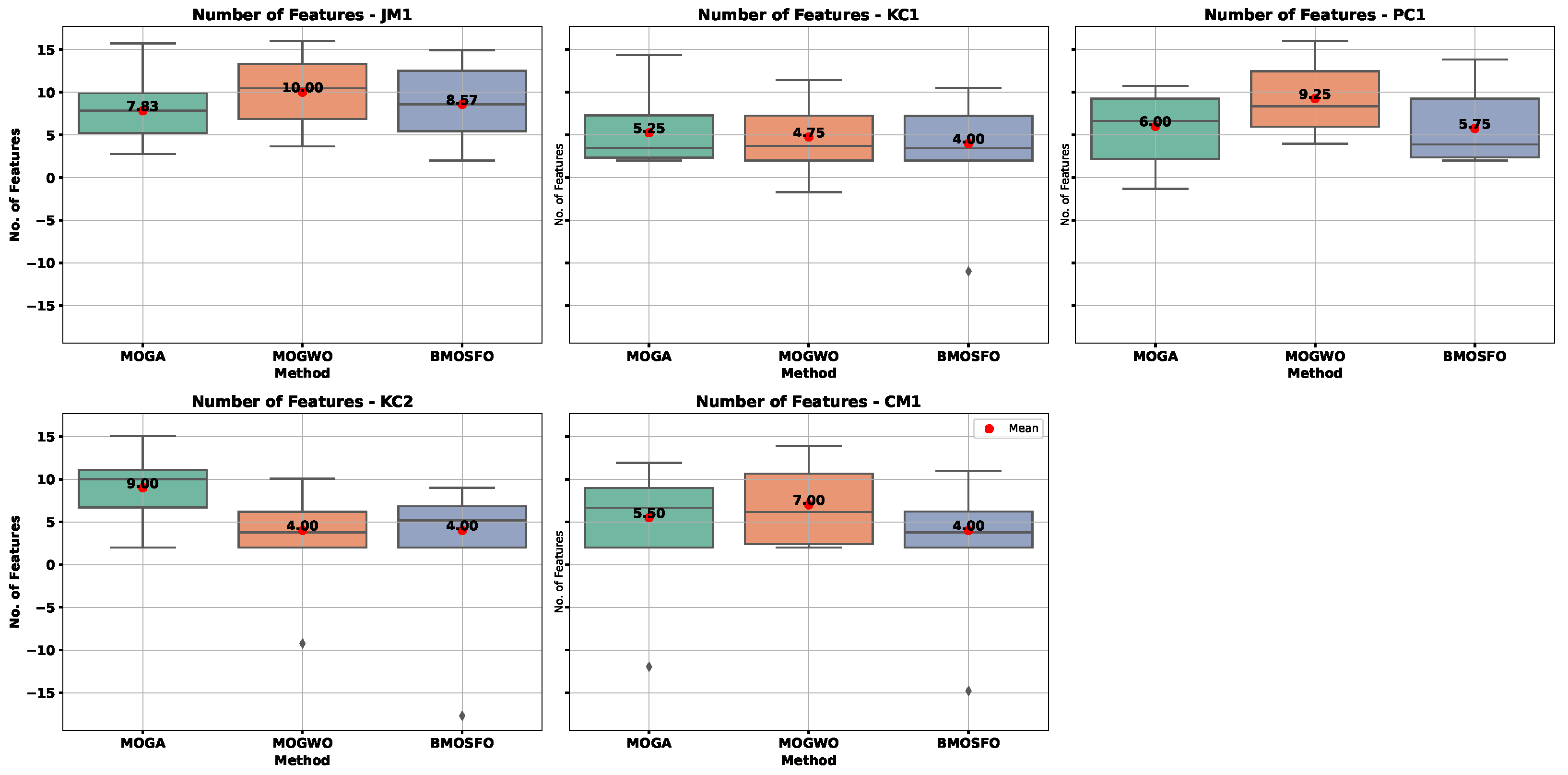
Figure 6 and Figure 7 show box plots of the objective functions over 20 independent runs. The relationship between selected feature count and classification accuracy was evident. BMOSFO consistently selected fewer features while achieving higher accuracy. MOGA, in contrast, tends to select more features with no accuracy gain, indicating redundancy. MOGWO typically had performance between that of MOGA and BMOSFO. These results confirm that optimal subset selection—rather than simply more features—is key to improved performance.

To further quantify Pareto front quality, the hypervolume metric was used.

Table 10. Hypervolume values of Pareto fronts for feature selection.

Datasets	MOGA	MOGWO	BMOSFO
JM1	0.21	0.28	0.30
KC1	0.29	0.22	0.37
PC1	0.28	0.19	0.40
KC2	0.20	0.22	0.34
CM1	0.17	0.22	0.36

presents the mean hypervolume values for all methods over 20 independent runs. Higher values indicated better convergence and diversity.

The hypervolume scores confirmed that BMOSFO dominated in all datasets, indicating better-balanced Pareto solutions. This reflected BMOSFO’s capacity to achieve superior trade-offs between feature count and classification accuracy.

The convergence plots for the five datasets are shown in Figure 8. BMOSFO consistently exhibited higher hypervolume throughout the iterations compared to MOGA and MOGWO. In the JM1 and KC2 datasets, convergence occurred after approximately 40 iterations, while, for KC1, convergence was achieved by the 30th iteration. For CM1 and PC1, improvements plateaued after the 40th iteration, indicating convergence before the 50th iteration.

The consistently higher hypervolume values for BMOSFO indicate its superior capability to maintain well-distributed and convergent Pareto solutions. This reflects BMOSFO’s effectiveness in achieving a balanced trade-off between maximizing classification accuracy and minimizing the number of selected features. The higher hypervolume scores also suggest that BMOSFO generates solutions that are closer to the true Pareto front, confirming its robustness in multi-objective optimization for feature selection.

To verify the statistical significance of BMOSFO’s superiority, the Wilcoxon signed-rank test was applied to the hypervolume values from the 20 independent runs.

Table 11. Wilcoxon test results on hypervolume.

BMOSFO vs.	MOGA		MOGWO
	p-Value	Significance	p-Value	Significance
JM1	0.00001	+	0.07	=
KC1	5.432 × ${10}^{-3}$	+	9.536 × ${10}^{-5}$	+
PC1	4.912 × ${10}^{-4}$	+	6.218 × ${10}^{-7}$	+
KC2	2.763 × ${10}^{-4}$	+	5.834 × ${10}^{-2}$	+
CM1	4.395 × ${10}^{-7}$	+	2.621 × ${10}^{-4}$	+

presents the results. BMOSFO significantly outperformed both MOGA and MOGWO in all cases except one, where the difference was not statistically significant (=). These results confirmed that BMOSFO’s improvements were consistent and not due to random variation.

The superior Pareto fronts achieved by BMOSFO can be attributed to its balanced exploration and exploitation strategies, which effectively navigated the search space for optimal feature subsets. By dynamically adjusting its search mechanism, BMOSFO maintained a well-distributed Pareto front, demonstrating its ability to achieve higher accuracy with fewer features compared to MOGA and MOGWO.

5.2.2. Impact of Feature Selection on Classification Accuracy

To determine the most representative solution from each Pareto front, the crowding distance (CD) metric was used.

Table 12. Selected features vs. classification accuracy.

Datasets	MOGA	MOGWO	BMOSFO
JM1	[16, 0.83]	[16, 0.83]	[12, 0.84]
KC1	[9, 0.85]	[8, 0.84]	[7, 0.85]
PC1	[3, 0.84]	[14, 0.92]	[8, 0.94]
KC2	[6, 0.79]	[7, 0.85]	[7, 0.92]
CM1	[9, 0.91]	[12, 0.90]	[7, 0.92]

presents the number of features and corresponding classification accuracy of the best solutions obtained from BMOSFO, MOGA, and MOGWO.

BMOSFO demonstrated consistent superiority by achieving higher accuracy with fewer features. Across all datasets, it yielded an average feature reduction of 43% and a classification accuracy gain of 5% compared to the alternatives. The key highlights include the following:

• In the JM1 dataset, BMOSFO selected 12 features and achieved an accuracy of 0.84, outperforming MOGA and MOGWO with 16 features.
• For the KC2 and CM1 datasets, BMOSFO achieved significant accuracy improvements of 13% (from 0.79 to 0.92) and 11% (from 0.81 to 0.92) by selecting only 7 out of 21 features.
• In the PC1 dataset, BMOSFO achieved the highest accuracy (0.94) with 8 features, surpassing MOGA and MOGWO, which required more features for comparable performance.

5.2.3. Analysis of Selected Features

Table 13. Selected features by BMOSFO for each dataset.

Dataset	Selected Features
JM1	Cyclomatic complexity, essential complexity, operators + operands (McCabe), volume, difficulty, time to write program, line count, count of lines of comments, count of blank lines, unique operands (Halstead), total operators, number of branches in flow graph
KC1	Halstead total operators + operands, McCabe design complexity, branch count, total operand, McCabe design complexity, Halstead program length, number of unique operators
PC1	McCabe design complexity, Halstead difficulty, branch count, Halstead number of delivered bugs, Halstead’s time estimator: time to write program, total number of operators + operands, McCabe design complexity, Halstead program length
KC2	McCabe design complexity, operators + operands, volume, Halstead difficulty, effort: Halstead effort to write program, Halstead’s time estimator: time to write program, count of lines that contain both code and comments
CM1	McCabe ‘cyclomatic complexity, McCabe ‘essential complexity, McCabe design complexity, Halstead program length, Halstead difficulty, Halstead line count, branch count of flow graph

lists the features selected by BMOSFO for each dataset. These include complexity metrics such as cyclomatic complexity and Halstead measures, known to be highly relevant to defect-prone modules.

The results highlight that BMOSFO effectively selects features related to code complexity, design structure, and maintainability, which are crucial factors influencing software defect prediction. The findings emphasize BMOSFO’s capability to balance feature reduction with high classification accuracy, making it a robust choice for multi-objective feature selection.

The selected features consistently included complexity metrics such as cyclomatic complexity, essential complexity, and Halstead measures, highlighting their strong correlation with defect-prone modules. These metrics capture critical aspects of code complexity, maintainability, and design quality, which significantly influence software defects. BMOSFO’s ability to prioritize these impactful features demonstrates its effectiveness in enhancing classification accuracy by focusing on the most relevant software metrics.

5.3. Discussion of the Classification Results After FS

This subsection analyzes the impact of feature selection using the proposed binary, multi-objective starfish optimizer (BMOSFO) on classification performance across five NASA datasets: JM1, KC1, PC1, KC2, and CM1. The relevant features identified by BMOSFO were used to create reduced datasets, as listed in Table 13. Multiple classifiers (KNN, SVM, DT, RF, LR, GNB, ANN, and Choquet fuzzy ensemble) were evaluated on these reduced datasets. Figure 9, Figure 10, Figure 11, Figure 12 and Figure 13 compare the classification results before (BFS) and after feature selection (AFS).

5.3.1. JM1 Dataset

The JM1 dataset contained 13,204 instances and 21 attributes. Figure 9 presents the classification results before and after feature selection for various models.

After feature selection, the accuracy and precision values increased for all classifiers. The most notable improvements were observed for the DT and ANN, whose accuracy values rose by 5% and 4%, respectively. The fuzzy ensemble method maintained the highest accuracy and precision, achieving an accuracy of 0.95 and precision of 0.94, representing a 4% improvement compared to the BFS results. These findings demonstrate that BMOSFO effectively identified the most relevant features, leading to enhanced classification reliability and generalization.

5.3.2. KC1 Dataset

The KC1 dataset consisted of 2109 instances and 21 features. Figure 10 provides the classification results before and after feature selection.

The accuracy values improved by up to 4% for several classifiers. The DT and ANN showed the most significant gains, increasing by 4% and 3%, respectively. The fuzzy ensemble method achieved the highest recall (0.99) and F1-score (0.97), indicating a balanced performance in precision and recall. These results demonstrate the effectiveness of BMOSFO in enhancing defect prediction accuracy by selecting the most relevant features.

5.3.3. PC1 Dataset

The PC1 dataset consisted of 1109 instances and 21 attributes. Figure 11 shows the classification results before and after feature selection.

Accuracy values increased for all classifiers except the SVM and RF, which remained unchanged. Notably, the DT and ANN achieved accuracy improvements of 4% and 3%, respectively. The fuzzy ensemble method recorded the highest F1-score (0.98) and recall (1.00), confirming its effectiveness in aggregating diverse classifiers for robust defect prediction. The results validate the capability of BMOSFO to enhance classification performance by optimizing feature selection.

Reducing dimensionality and eliminating redundant features through feature selection improves classification performance. However, the impact of specific features varies by classifier. This work selected features optimized for KNN, which relies on distance-based similarity and is highly sensitive to feature selection. Conversely, SVM and random forest inherently handle irrelevant features better due to their kernel-based and ensemble learning approaches, respectively. This explains why in datasets like PC1, their accuracy remained unchanged after feature selection.

Although increasing accuracy is the main objective of feature selection, it also improves model interpretability, computational efficiency, and overfitting reduction. Even in cases where accuracy remains stable, feature selection reduces training time, simplifies models, and enhances generalization. Exploring adaptive feature selection strategies that dynamically adjust to different classifiers could further increase applicability.

5.3.4. KC2 Dataset

The KC2 dataset consisted of 522 instances and 21 attributes. Figure 12 compares the classification results before and after feature selection.

After feature selection, the KNN and ANN exhibited remarkable accuracy improvements of 13% and 10%, respectively. The fuzzy ensemble method delivered a balanced performance, achieving 5% higher precision, 2% more recall, and a 3% improvement in F1-score, albeit with 1% lower accuracy compared to the BFS results. These findings highlight the superior capability of BMOSFO in selecting the most relevant features for improved classification reliability.

5.3.5. CM1 Dataset

The CM1 dataset consisted of 498 instances and 21 features. Figure 13 presents the classification results before and after feature selection.

BMOSFO enhanced accuracy for all classifiers except the SVM and LR, with the latter maintaining the same accuracy level. Notably, the DT and ANN achieved accuracy gains of 4% and 3%, respectively. The fuzzy ensemble method demonstrated the most consistent performance, achieving the highest F1-score (0.96) and accuracy (0.93). These results underscore the effectiveness of BMOSFO in enhancing classification performance by optimizing feature selection.

5.3.6. Execution Time Comparison

The average execution time across the five NASA datasets is recorded in

Table 14. Average execution time across classifiers and feature selection methods.

Methods	Average Execution Time (s)
Base Classifiers with Full Feature Set	128
Feature Selection using BMOSFO	73.45
Base Classifiers after Feature Selection	65.82
Ensemble Classifier with Choquet Fuzzy Integral	16.23

. While feature selection with BMOSFO introduced computational overhead, it optimally reduced irrelevant features compared to filter-based methods. Additionally, it significantly decreased classifier training time, balancing the extra cost incurred by the ensemble approach.

Ensemble models provide substantial benefits in classification accuracy, robustness, and generalization, despite their computational cost. They reduce overfitting, mitigate individual model biases, and enhance prediction stability—critical for software defect prediction where accurate fault detection is essential. Feature selection methods further balance computational cost by lowering dimensionality, making ensemble models a reliable and effective approach for high-dimensional classification tasks.

5.3.7. Discussion of Classification Improvements

The comparative analyses before and after feature selection demonstrate that BMOSFO significantly enhanced classification performance across all five datasets. The fuzzy ensemble method consistently delivered the highest accuracy and F1-scores, demonstrating its robustness in aggregating diverse classifiers. Key observations include the following:

• Accuracy improvements ranged from 1% to 13%, with the most substantial gains observed for KNN and the ANN in the KC2 dataset.
• The fuzzy ensemble method exhibited consistent performance across all metrics, highlighting its ability to leverage classifier diversity for improved generalization.
• The DT and ANN showed remarkable accuracy enhancements, reflecting their adaptability to the optimized feature sets generated by BMOSFO.
• The SVM and LR maintained stable accuracy levels but showed minimal improvement, suggesting their limited sensitivity to feature selection.

The consistent performance gains achieved through BMOSFO across all datasets validate its robustness in optimizing feature selection for defect prediction. By effectively balancing feature reduction and classification accuracy, BMOSFO not only enhances predictive performance but also improves computational efficiency. These findings demonstrate the practicality of BMOSFO in real-world software defect prediction scenarios, where high-dimensional data and class imbalance present significant challenges.

6. Conclusions and Future Work

This study presented a novel approach to software defect prediction by developing a binary, multi-objective starfish optimizer (BMOSFO) for feature selection. The primary objective was to enhance the efficiency and effectiveness of fault predictors by selecting the most relevant features from NASA datasets. By optimizing two conflicting objectives—minimizing the number of selected features and maximizing classification accuracy—BMOSFO demonstrated superior performance compared to conventional feature selection methods, including MOGA and MOGWO.

The experimental evaluation on five NASA datasets (JM1, KC1, PC1, KC2, and CM1) showed that BMOSFO consistently outperformed other methods, achieving the highest hypervolume values and generating Pareto solutions closer to the true Pareto front. The selected features included critical metrics such as design complexity, total number of operators and operands, time to build the program, lines of code, number of lines containing both code and comments, number of branches, and sum of operands. These features were strongly correlated with defect-prone modules, highlighting their importance in enhancing software defect prediction.

By leveraging an ensemble approach based on the Choquet fuzzy integral, classification performance was further improved. The fuzzy ensemble method effectively aggregated multiple predictive models, enhancing interpretability and reliability while reducing overfitting risks. It consistently delivered the highest accuracy and F1-scores across all datasets, validating its robustness in aggregating diverse classifiers.

Despite BMOSFO’s superior performance in feature selection and defect prediction, several limitations and potential avenues for future research were identified. This study focused on NASA datasets, which primarily contain source code-related metrics. Future research could investigate the applicability of BMOSFO to a broader range of datasets, including those incorporating architectural, design-level, or service-oriented metrics.

Additionally, the initial population of BMOSFO was generated randomly. Incorporating advanced population initialization techniques, such as knowledge-based or heuristic-guided initialization, could enhance convergence speed and solution diversity. Furthermore, while this study employed traditional machine learning classifiers, integrating BMOSFO with deep learning models such as convolutional neural networks (CNNs) and long short-term memory (LSTM) networks could further improve defect prediction accuracy.

Future work could also explore alternative ensemble learning techniques, including stacking, boosting, and bagging, to further enhance classification performance. Additionally, given BMOSFO’s demonstrated robustness, its applicability to other classification domains—such as medical diagnosis, fraud detection, and financial risk prediction—warrants investigation [63].

Combining BMOSFO with other evolutionary or swarm intelligence algorithms (e.g., genetic algorithms, particle swarm optimization) could strengthen its exploration and exploitation capabilities. Finally, integrating explainable artificial intelligence (XAI) techniques into the fuzzy ensemble method could enhance interpretability, fostering greater trust and adoption among stakeholders in predictive modeling.