1. Introduction
Truncated probability distributions (TPD) arise when the domain of a probability distribution is restricted to a specific range, effectively excluding certain values or intervals from the distribution. The motivation of TPD is to enhance sampling, parameter inference, fast convergence in the related region, which will lead to a robust estimation. These modifications alter the fundamental properties of the original distribution, such as its mean, variance, and moments, to reflect the effects of truncation. Existing models for bounded data, that include unit-domain or truncated distributions, suffer from restricted intervals, inflexible parameterization, or normalization complexities. Truncated distributions are ubiquitous in real-world applications where the data naturally adhere to specific bounds, such as in censored data sets, physical measurements constrained by limitations of instruments, or predefined policy thresholds. For example, in medical statistics, ref. [
1] used truncated distributions to model survival times when data collection is limited to a specific observation window. Similarly, environmental science leverages truncated models to study phenomena like precipitation levels, which naturally fall within bounded ranges [
2]. In many other real-world scenarios, proportions, probabilities, financial decisions, or measurements within a specific range naturally occur within bounded domains [
3].
The concept of truncation extends to a wide variety of probability distributions, including the normal, exponential, and Poisson distributions (see, [
4]). Among these, the truncated normal distribution holds particular importance due to the centrality of the normal distribution in the statistical theory and applications. Early work by [
5] laid the foundation for understanding the properties of truncated distributions, including their moments and implications. This was followed by [
6], who provided comprehensive derivations for the mean and variance of the truncated normal distribution and explored their dependency on truncation limits. For a review regarding the properties of the truncated normal distribution, we refer to [
7]. The truncated normal distribution has been applied in fields ranging from genetics to finance. In reliability engineering, it is used to model lifetimes of components when failures outside a specific range are unobservable [
2].
Truncated or unit domain models effectively capture processes or behaviors constrained by known limits, ensuring realistic outcomes and avoiding impossible values. Models defined on bounded intervals provide meaningful parameter estimates that align with the domain’s restrictions. Using truncated domains prevents predictions from falling outside feasible or observable ranges, enhancing model reliability, and decision-making in practical applications. There are fewer distributions on truncated domain than on
, for example, uniform on
, U-quadratic on
, truncated normal on
(see, [
7]), arc-sine on
(see, [
8]), and Pareto distribution on
(see, [
9]). Recently, new generalized uniform proposed by [
10] and Mustapha type III by [
11], are additional instances, among others.
This work is inspired by the significant impact of the half-normal distribution across various fields of study. For instance, [
12] recently proposed a modified half-normal distribution, while [
13] introduced an extension of the generalized half-normal distribution. The unit-half-normal distribution was explored by [
14], and [
15] developed a model based on the half-normal distribution to adapt financial risk measures, such as value-at-risk (VaR) and conditional value-at-risk (CVaR), for scenarios with solely negative impacts. Additionally, ref. [
16] proposed an estimation procedure for stress–strength reliability involving two independent unit-half-normal distributions, and [
17] discussed objective Bayesian estimation for differential entropy under the generalized half-normal framework. Furthermore, ref. [
18] examined inference for a constant-stress model using progressive type-I interval-censored data from the generalized half-normal distribution, among other contributions.
In this paper, we introduce the truncated -half-normal distribution, a novel probability model defined on the bounded interval . The proposed distribution characteristics are analytically tractable statistical properties, making it versatile for modeling various density shapes within truncated domains. Parameter estimation was performed using a hybrid approach: maximum likelihood estimation (MLE) and a likelihood-free-like technique. We supported the estimation method by sensitivity analysis using simulated data, and an optimal estimation algorithm, to determine the best estimates. The exceptional performance of the proposed model is demonstrated through applications to real-world data.
The truncated ()-half-normal distribution addresses these gaps by transforming the half-normal distribution via a new ratio mapping, eliminating normalization constants and enabling flexible modeling on any interval (). Its parameters directly control bounds , interval length , and dispersion , offering interpretability and analytical tractability. Unlike Beta, Kumaraswamy and Topp–Leone models, it inherits the asymmetry and tail behavior of half normal, proving superior in real-world data applications providing lower value of goodness-of-fit statistics. Finally, although the support of the proposed distribution is defined over a general bounded interval with , in most empirical applications may be appropriate. However, allowing increases the generality of the model, facilitates applications that involve transformed or standardized data, and aligns with the theoretical origins of the model as a transformation of a symmetric normal variable.
The structure of the paper is as follows:
Section 2 introduces the formulation of the proposed model and its statistical properties.
Section 3 discusses maximum likelihood estimation method and provides sensitivity analysis on the parameters.
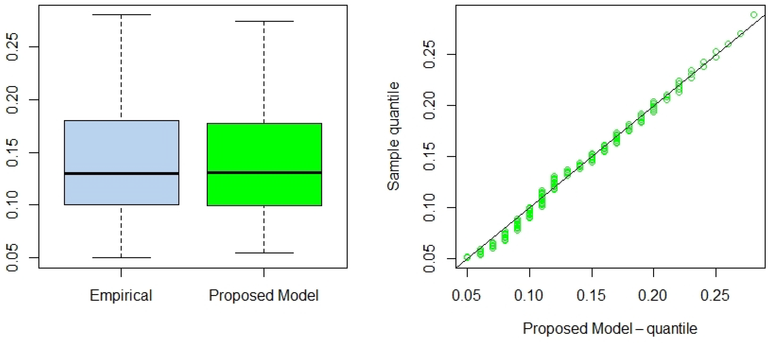
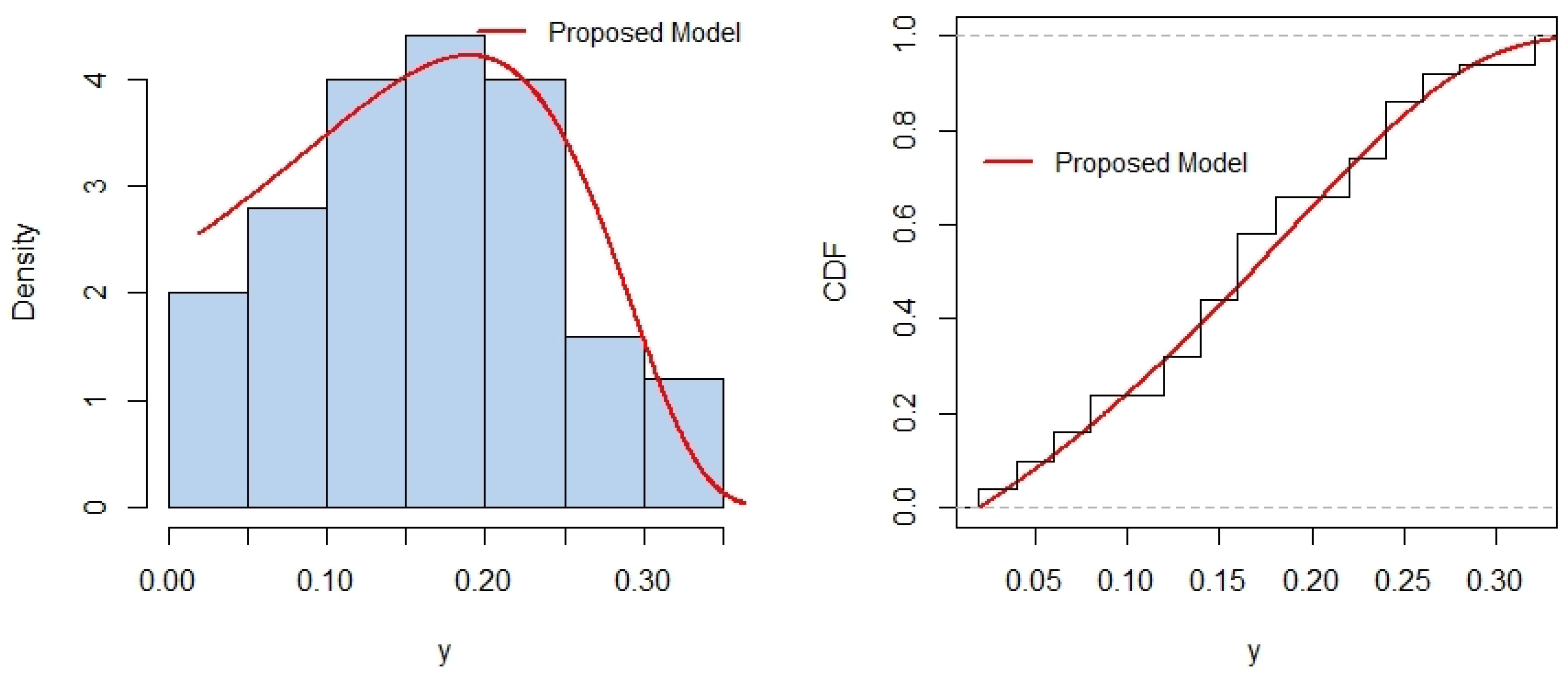
Section 4 presents two illustrative real-world data applications. Finally,
Section 5 concludes the paper with a summary of findings and implications.
2. Definition and Properties
Assume that the random variable
X is normally distributed, with mean
and variance
as parameters. Note that, the random variable defined as the absolute value of
X, i.e.,
, follows the half-normal distribution (HN), originally suggested by [
19] for creating centile charts. Now, let
denotes the cumulative distribution function (CDF) associated with
X. The aim is to introduce a new random variable, denoted by
Y, defined on
, where
, with
and
.
Thus, from the distribution of
X, one can define the CDF of a “new” variable Y as follows
Remark 1. Using the symmetric properties of the normal distribution of X, for all , one can see that Furthermore, one can deduce thatwhere (which follows a normal distribution with u as mean and σ as standard deviation). Proposition 1. Based on the above results, one can see that Proof. Let
y be a real value, such that
. Thus, we have
□
Remark 2. defined in (
1)
is a novel transformation analogous to the odd ratio concept, but constructed using absolute value. Thus, one can easily see that has as support, that is, the choice maps to , ensuring bounded support. Furthermore, for all , the CDF associated with is defined as followswhere denotes the CDF associated with X. The classic procedure for producing a truncated distribution, is a conditional distribution that results from restricting the domain of some other probability distribution. Explicitly, suppose that
X is a random variable with
as support (in general,
I is an open interval). Thus, in order to define a new random variable, denoted
Y, with bounded support
, from
X, we define
Y as follows
Therefore, the PDF and CDF associated with
Y are, respectively, given by
and
where
(resp.
) denotes the PDF (resp. CDF) associated with
X and
is an indicator function. One of the weak points of this classic procedure is that the normalization constant, given by
, of the new distribution depends on
(which may not have an explicit form in some cases, in particular when
X is a normal random variable). This can have a negative impact, for example, for managing the maximum likelihood function and consequently the expansions of the likelihood ratio tests. To overcome these difficulties we mixed two approaches. First, we used the composed CDF, originally proposed by [
20] to created a distribution with support on
from a positive random variable, and the linear transformation of unit transform random variable, usually used to change support of a random variable. Indeed, based on Proposition 1, one can see that
Y is an affine function of a unit transform random variable
Note that, even if the support of
(i.e.,
) is independent of
b, this parameter play an important role in the construction of
, which makes a noticeable difference from the basic rescaling technique. Furthermore, one can say that
follows the HN distribution. Thus,
can be seen as a “modified version” of the unit-HN distribution, originally introduced by [
14] (indeed, for
,
is exactly the unit-HN distribution).
Remark 3. Indeed, when , the distribution of the introduced variable Y can be seen as a simple linear transformation of the Unit-HN distribution. This transformation allows that Y has as support.
While the support of the proposed distribution on may resemble that of a truncated normal, the two models differ substantially. The truncated normal relies on a renormalization of the classical normal distribution over a bounded interval, requiring computation of cumulative distribution values. In contrast, the proposed model is based on a nonlinear transformation of an HN variable, yielding a closed-form density that avoids normalization constants. Moreover, the shape of the distribution can be flexibly controlled via the ratio , enabling a useful class of behaviors than the truncated normal.
Finally, from Remark 1, one can see that
where
(In other words,
has a folded normal distribution (if
, then
has a half-normal distribution)).
Based on Remark 1, one can write the PDF that associated with
Y as follows
where
denotes the PDF associated with
X. The transformation of the support of
X using the nonlinear mapping
transform the density shape and stretches the half-normal density dynamically based on
a, allowing the PDF of
Y to adapt its shape within
, additionally, it may exhibit heavier tails or sharper peaks near
b which can provide more flexibly to the proposed model. The parameter
b scales the proposed transformation, affecting the rate at which probability accumulates near
v, unlike other truncated models such as truncated normal on
in which the upper bound b is like a hard cut-off. Now, using (
3) and results of Remark 1, the survival function (S.F.) and hazard rate function (H.R.F.) associated with
Y, are given, for all
, respectively, by
and
where
and
denote, respectively, the S.F. and the H.R.F. associated with
X.
Proposition 2. The PDF of the proposed distribution in (3) is unimodal with mode at either for all or for some, Proof. We show that
has a real root. Recall that the function
is defined by
Thus, one can find that
We can solve
directly from (
4) to determine the possible root of
as follows. Let
, then
By applying quadratic equations formula in (
5), we get
Hence,
or
Finally, we can claim that there exist a root among
which implies that
has unimodal density. □
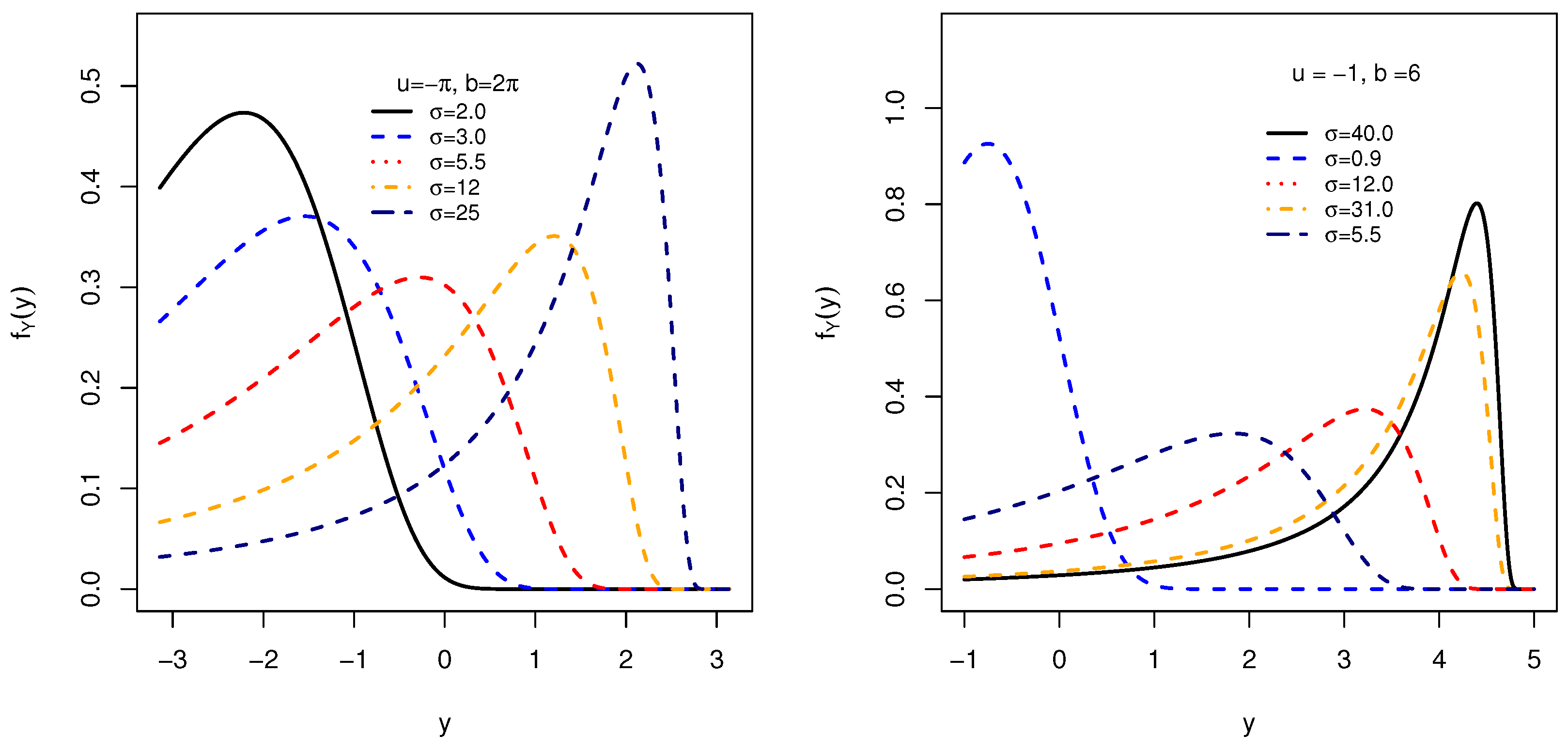
Figure 1 illustrates some possible shapes of the PDF in (
3) associated with the variable
Y, when
,
(i.e.,
Y has
as support), and for some selected values of the parameter
(indeed, due to (
2), on the right part of
Figure 1 we choose
values such that
is rather weak (≤1), and
values such that
is large (>1)).
Figure 1 confirms the results mentioned in the previous section. In particular, these graphical results show the usefulness of the distribution of
Y in terms of dispersion, asymmetry (left and right skewed) and flattening, which adopt various phenomena across the applications.
2.1. The Moment of Y
The moment of Y is defined to be . In this section, we present the calculation of this measure. Specially, we focus on the first four moments, which usually used to study the dispersion and the form (asymmetry and kurtosis) of the distribution.
Remark 4. Using Newton’s Binomial formula and based on (
1)
, one can write the moment of Y as follows Furthermore, based on the Proposition 2.1 of [
14], one can write the expression of the
moment of
as follows
Remark 5. Based on the properties of HN distribution (for details, see, e.g., [5,21]), for all , we haveA closed-form expression of the raw moment of the proposed distribution in terms of elementary functions is not tractable due to the bounded transformation involved, it is nonetheless possible to express it symbolically using the Meijer G function a highly general class of special functions encompassing many classical functions (e.g., exponential, logarithmic, Bessel, hypergeometric). Indeed, Meijer G function is defined through a complex contour integral representation (see [22]). This expression allows general and symbolic computation of moments for a wide range of parameter values (for more details, see [23,24,25]). Explicitly, by introducing the substitution , the moment integraltransforms into an expression involving the integrand , for which Meijer G representations are available:Thus, the moment can be formally written as a weighted integral involving Meijer G functions. Thus, the value of , for all , can be solved numerically by using, for example, the integrate()
function of the
stats
package of
R (see [26]). This representation provides a useful foundation for further analytical generalizations and asymptotic studies. Thus, based on Remark 4 and Equation (
6), one can deduce that
We can deduce that, the moments depend on
, enabling flexible tail control. Consequently, the mean, variance, coefficient of variation (CV), skewness (CS), and kurtosis (CK) coefficients are, respectively,
and
Based on Remark 5,
Table 1 presents the numerical calculation for coefficient of variation (CV), skewness (CS), and kurtosis (CK) coefficients of the variable
Y with different set of values associated with the parameters
and
b, with
. Note that CS and CK coefficients are independent of
u. However,
u could play an important role for the CV measures (indeed, obviously when
u sufficiently large, we have that the CV is close to zero, which implies that the distribution of
Y is concentrated around its mean (which will also be very large).
Thus, for , one can observe that when increases, then the CV decreases (therefore, we have a weak dispersion around the mean). Moreover, independently of the value of u, one can see also that when increases, then we obtain a negative CS, which indicates a longer tail to the left of the distribution of Y. Finally, one can deduce that there exists an interval of positive value (denoted by ) such that if belongs to it, then the CK value is less than 3, otherwise the CK value is greater than 3. Then, the value of plays an important role in identifying the level of flattening of the distribution of Y (compared to the normal distribution).
Proposition 3. The moment generating function of the variable Y is given by Proof. First, recall that
Based on the results of this section and the Proposition 2.2. of [
14], we have
□
2.2. Random Data Sampling
This section outlines the quantile function associated with the proposed model, which is essential for generating random samples. The quantile function is crucial for determining different percentiles of a distribution, such as the median, and is a key component in creating random variables that conform to a given distribution. Additionally, in non-parametric testing, the quantile function helps in identifying critical values for test statistics, thereby enhancing the robustness of statistical analysis.
Proposition 4. The quartile function (QF) associated with Y is defined as followswhere denotes the QF related to X. Proof. Let
and
. Thus, we have
□
An alternative way that involves root finding is developed and very effective, the step by step algorithm is provided below in the description of Algorithm 1, and the
R codes can be found in the
Appendix A.
| Algorithm 1 Step-by-Step Algorithm for the random data sampling. |
| 1. | Define the parameters for the quantile function: |
| 2. | Define the PDF as the in (3). |
| 3. | Define the CDF as the numerical integral of the PDF from u to y: |
| | . |
| 4. | The quantile function is to find the value of y such that: |
| | |
| 5. | Solving the equation in step 4 by using the root-finding algorithm (e.g., uniroot in R). |
5. Conclusions
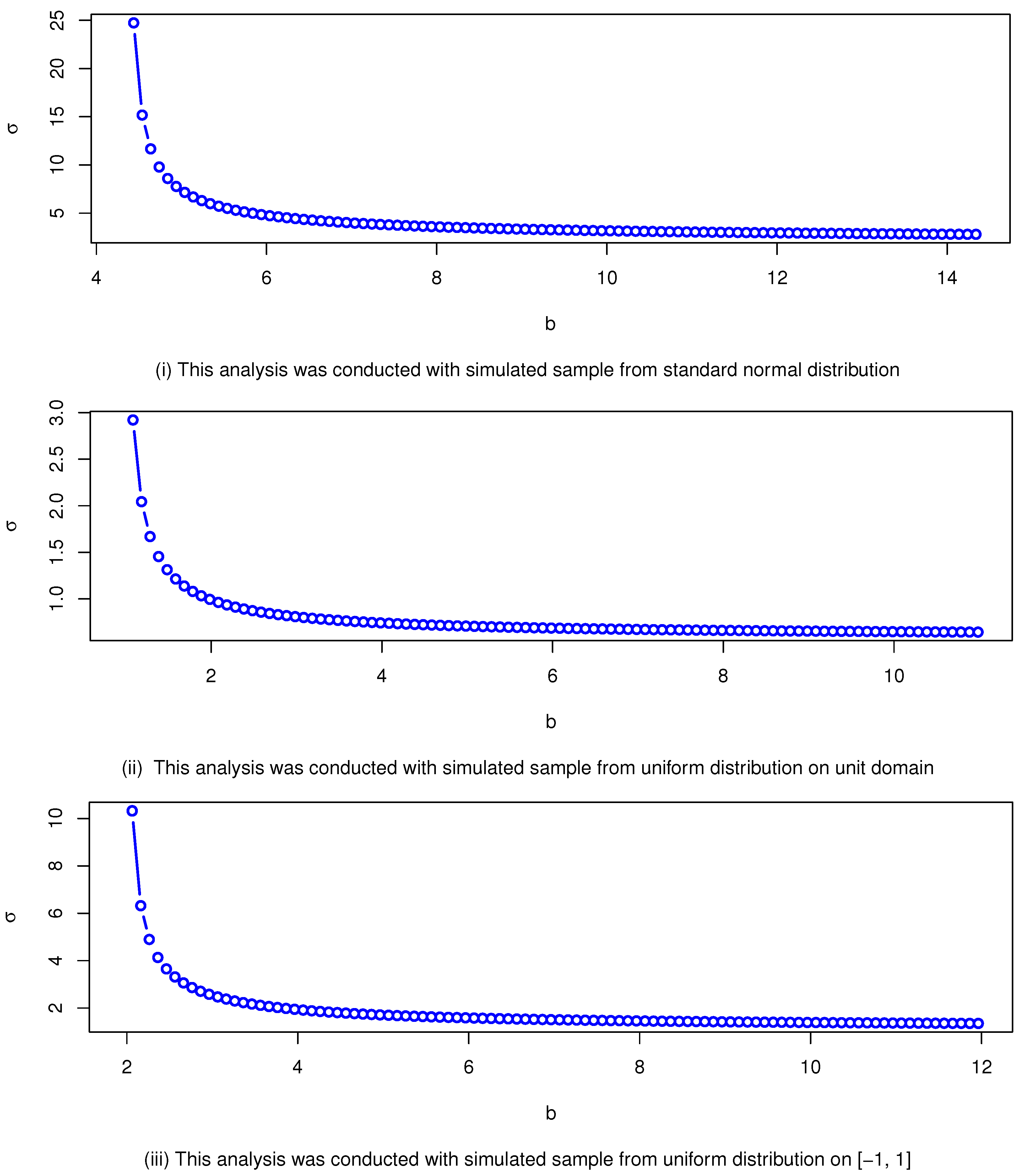
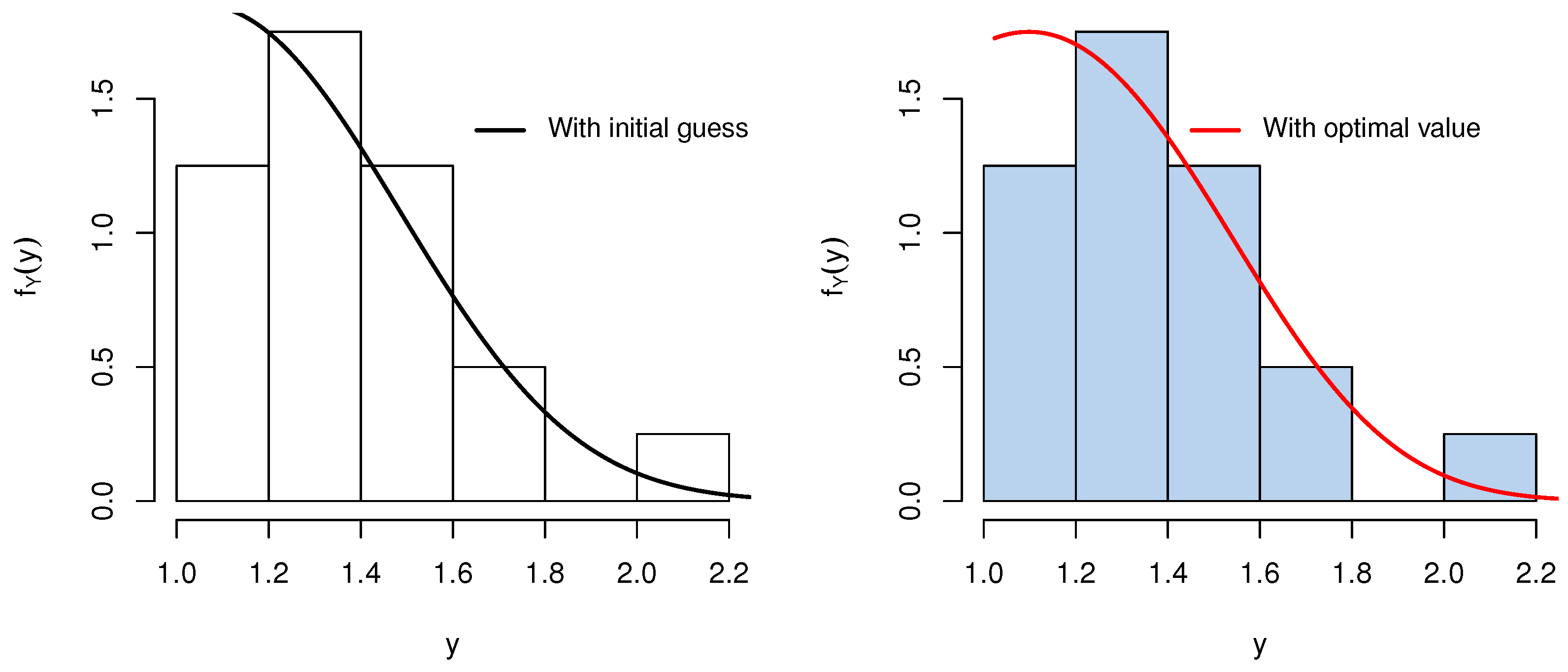
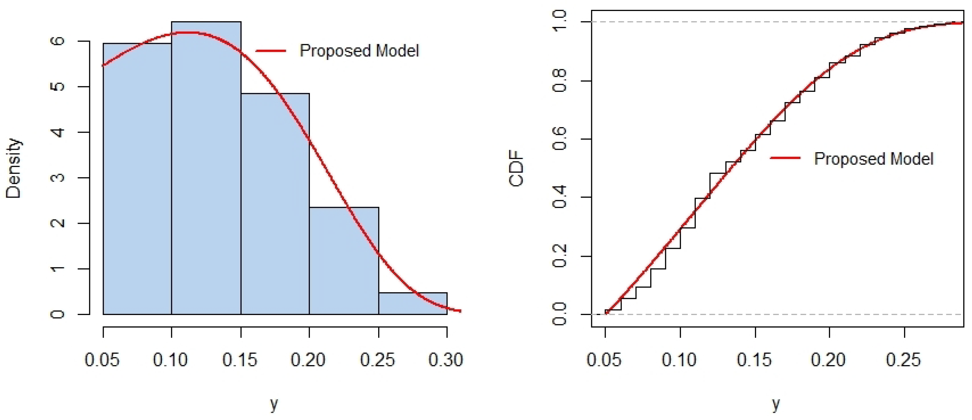
In this paper, we introduced the truncated -half-normal distribution, a novel probability model for bounded domains, addressing the need for realistic and analytically tractable models in constrained scenarios. Several properties of the model, including its cumulative distribution function, probability density function and its possible shapes, survival function, hazard rate, and moments, were rigorously derived and analyzed. Parameter estimation was performed using a hybrid approach: MLE for and a likelihood-free-like technique for b. We supported the results using sensitivity analysis, and an optimal estimation algorithm, to determine best estimates. The MLE of depends strongly on , as sensitivity analysis reveals that initially starts high and decreases rapidly with increasing b, particularly near some threshold value, leading to large variations. Beyond the threshold, changes in b have a diminishing impact, and converges to a stable value, indicating reduced sensitivity for large b. Hence, the utilization of the proposed algorithm helps to determine the optimal estimates. In addition, simulated data is used to demonstrate the accuracy and importance of the proposed hybrid algorithm. Applications to two real-world data sets demonstrated the superior performance of the proposed model compared to widely used alternatives, with better fit across metrics like AIC, BIC, CAIC, KS, AD, and CvM statistics. These results highlight the versatility and robustness of the -half-normal distribution for modeling data with bounded support. We note that while the formulation permits negative lower bounds (), its empirical relevance depends on the nature of the data. In contexts involving standardized or signed measurements, this generalization may prove useful. In strictly positive domains, should naturally be enforced. An interesting avenue for future research is the extension of the proposed bounded half-normal distribution to a regression framework. In such a setting, the location (e.g., via a transformation of the interval ), the scale parameter , or the shape parameter b could be modeled as functions of covariates. This would allow practitioners to model bounded response variables that exhibit half-normal-like asymmetry while accounting for explanatory variables. Such an extension could be pursued within both classical and Bayesian inferential paradigms, potentially using maximum likelihood or Bayesian hierarchical models. The development of suitable link functions, estimation procedures, and diagnostics tailored to this bounded setting would form an important next step.


 ,
, 


