A Meta-Learning Approach for Estimating Heterogeneous Treatment Effects Under Hölder Continuity

Abstract

Estimating heterogeneous treatment effects plays a vital role in many statistical applications, such as precision medicine and precision marketing. In this paper, we propose a novel meta-learner, termed RXlearner for estimating the conditional average treatment effect (CATE) within the general framework of meta-algorithms. RXlearner enhances the weighting mechanism of the traditional Xlearner to improve estimation accuracy. We establish non-asymptotic error bounds for RXlearner under a continuity classification criterion, specifically assuming that the response function satisfies Hölder continuity. Moreover, we show that these bounds are achievable by selecting an appropriate base learner. The effectiveness of the proposed method is validated through extensive simulation studies and a real-world data experiment.

1. Introduction

Causal inference plays a pivotal role across a wide range of scientific disciplines. With the rapid advancement of big data technologies, researchers now have access to more information than ever before, enabling more accurate estimation of causal effects. A central task in this field is the estimation of heterogeneous treatment effects (HTEs), which seeks to quantify how treatment effects vary across individuals or subpopulations. This is particularly critical in domains such as precision medicine and targeted policy-making, where practitioners—such as doctors, policymakers, and researchers—aim to determine whether newly developed treatments or interventions produce the desired outcomes for different groups.

As research in causal inference has progressed, it has become increasingly clear that average treatment effects (ATEs) may mask significant heterogeneity at the individual level. As a result, growing attention has been devoted to the estimation of conditional average treatment effects (CATEs), which aim to capture individual-level causal effects conditional on observed covariates.

Early approaches to estimating CATEs include semi-parametric models, such as partial linear models [1,2] and additive models [3], as well as classical non-parametric methods [4]. In addition, several weighting-based methods have been proposed, including inverse probability weighting (IPW), augmented IPW (AIPW) [5,6,7], and propensity score optimization techniques [8]. These traditional methods are supported by mature theoretical foundations but often rely on restrictive modeling assumptions, which limit their flexibility in capturing complex real-world data structures.

With the rise of machine learning, researchers have developed a variety of flexible, data-driven methods for estimating CATEs. Ref. [9] introduced a model-free meta-learning algorithm, which was further extended by [10] through a general framework that includes the Slearner and Tlearner [11,12], and later the Xlearner. Other notable contributions include the Rlearner based on Robinson decomposition [13], Athey’s Causal Forest [14], and the Double Machine Learning (DML) framework [15], which utilizes Neyman orthogonality and cross-fitting to reduce sensitivity to nuisance parameters. The Doubly Robust Learner (DRL) [16] and the unifying framework proposed by [17]—which incorporates the L1 loss to enhance robustness—further broaden the scope of meta-learning-based estimators.

These modern approaches leverage the flexibility of machine learning to model complex functional relationships and have demonstrated strong empirical performance. However, despite their practical success, most theoretical analyses of these methods rely on strong smoothness assumptions, such as requiring the response function to lie in a reproducing kernel Hilbert space (RKHS) or satisfy Lipschitz continuity. While these assumptions facilitate theoretical derivations, they may not hold in many real-world applications.

Among the existing meta-learning methods, the Xlearner has demonstrated strong empirical performance, particularly in scenarios with covariate unbalance and unequal treatment assignment rates. Its design leverages different base learners for treated and control groups, which allows it to adapt well to unbalanced datasets and heterogeneous response surfaces [10]. These features make Xlearner one of the most widely used and practically effective methods in CATE estimation. However, despite its strengths, Xlearner still faces two main challenges. First, as noted by [10], its reliance on propensity scores as weighting functions can limit its flexibility, particularly in complex or high-dimensional data settings. Second, most of its theoretical guarantees rely on the assumption that the underlying response functions are Lipschitz continuous, which may not hold in many practical scenarios where the functions are less smooth or exhibit discontinuities.

To address the limitations of fixed-weight designs and the error accumulation inherent in the Xlearner, while preserving its structural advantages, we propose a novel meta-learning method called RXlearner. This method incorporates a data-driven, covariate-dependent weighting mechanism that adaptively combines pseudo-treatment effect estimates. By doing so, RXlearner enhances the model’s flexibility in capturing complex response patterns and mitigates cumulative errors across estimation stages.

We rigorously establish the theoretical properties of RXlearner by deriving a non-asymptotic error bound under the assumption that the response function satisfies Hölder continuity, a milder and more general condition than those typically assumed in the existing literature. The effectiveness of RXlearner is further demonstrated through extensive simulation studies and a real-world application. While the inherent variability in the data makes the identification of a universally optimal estimator elusive, our results show that RXlearner delivers consistently competitive and robust performance across a broad range of scenarios.

The remainder of this paper is organized as follows. Section 2 introduces the model assumptions and presents the RXlearner algorithm. Section 3 develops the theoretical analysis of the estimator, where we derive non-asymptotic error bounds under Hölder continuity. To evaluate the practical effectiveness of the proposed method, Section 4 reports results from simulation studies, and Section 5 applies RXlearner to a real-world dataset. Section 6 concludes the paper with further discussions and directions for future research. Technical proofs are provided in Appendix A.

2. Methodology

2.1. Models and Assumptions

We consider the estimation of the conditional average treatment effect (CATE) under the potential outcomes framework of Neyman–Rubin [18,19]. Let $W\in \{0,1\}$ be a binary treatment indicator, and for each unit i, let $Y_i^1$ and $Y_i^0$ denote the potential outcomes under treatment and control, respectively. Let $X_i\in {\mathcal{R}}^p$ represent the p-dimensional covariates. We assume that the data are generated independently from a distribution $\mathcal{P}\in \mathcal{D}$, such that

$$(Y_i^1,Y_i^0,X_i,W_i)\sim \mathcal{P}.$$

Under the Stable Unit Treatment Value Assumption (SUTVA) [20], the observed outcome is given by

$$Y_i=\mathbb{I}(W_i=1)Y_i^1+\mathbb{I}(W_i=0)Y_i^0,$$

where $\mathbb{I}(·)$ denotes the indicator function. The observed dataset is denoted as

$$\mathcal{D}={\left\{(Y_i,X_i,W_i)\right\}}_{i=1}^N.$$

We define the response functions as

$${\mu }_1\left(x\right)=\mathbb{E}[Y^1\mid X=x],{\mu }_0\left(x\right)=\mathbb{E}[Y^0\mid X=x],$$

and the corresponding conditional average treatment effect (CATE) function is

$$\tau \left(x\right)=\mathbb{E}[Y^1-Y^0\mid X=x]={\mu }_1\left(x\right)-{\mu }_0\left(x\right).$$

To simulate observed outcomes, we further adopt an additive noise model

$$Y_i={\mu }_{W_i}\left(X_i\right)+\sigma {ϵ}_i.$$

The variance parameter $\sigma$ controls the noise level and is varied across simulation scenarios.

The propensity score, i.e., the probability of receiving treatment conditional on covariates, is defined as

$$\begin{array}{c}\hfill e\left(x\right)=\mathbb{P}(W=1\mid X=x).\end{array}$$

(1)

Our goal is to estimate $\tau$ with an estimator $\widehat{\tau }$, and to evaluate its performance under the expected mean squared error (EMSE), defined as

$$\mathrm{EMSE}(\mathcal{P},\widehat{\tau })=\mathbb{E}\left[{(\tau \left(\mathcal{X}\right)-\widehat{\tau }\left(\mathcal{X}\right))}^2\right].$$

Here, we follow the EMSE definition proposed in [10], where $\mathcal{X}\sim \mathsf{\Lambda }$ and $\mathcal{X}$ is assumed to be independent of $\widehat{\tau }$. In our implementation, this assumption is addressed via a sample-splitting strategy: the estimator $\widehat{\tau }$ is trained on one subset of the data, and EMSE is evaluated on an independent test sample drawn from the same distribution. This design ensures that $\widehat{\tau }\left(\mathcal{X}\right)$ is independent of $\mathcal{X}$ at evaluation time. Consequently, $\mathsf{\Lambda }$ corresponds to the marginal distribution of the evaluation sample.

To establish the theoretical properties of the estimator, we make the following standard assumptions.

Assumption 1

(Ignorability). The treatment assignment $W_i$ is independent of the potential outcomes $(Y_i^1,Y_i^0)$ conditional on the covariates $X_i$, i.e.,

$$(Y_i^1,Y_i^0)\perp W_i\mid X_i.$$

Assumption 2

(Positivity). The propensity score is bounded away from 0 and 1, i.e., $e\left(x\right)\in (0,1)$ for all $x\in \mathcal{X}$.

Assumption 3

(Conditionally Independent Errors). The errors are independent of treatment assignment given the covariates, i.e., ${ϵ}_i\perp W_i\mid X_i$. We further assume that $\mathbb{E}[{ϵ}_i\mid X_i]=0$ and that the conditional variance of the errors exists.

Remark 1.

Assumption 3 states that the error term ${ϵ}_i$ is conditionally independent of the treatment assignment $W_i$ given the covariates $X_i$. This assumption ensures that the estimation of nuisance functions (such as the outcome regressors and the imputed treatment effect differences in the first stage) is unbiased. It is a standard condition in many meta-learner frameworks, including the Xlearner. In our RXlearner, this assumption supports the consistency of the refined weighting strategy. While the assumption may be restrictive in practice, it provides a clean theoretical foundation. We acknowledge this limitation and leave the relaxation of this assumption for future exploration.

2.2. Meta-Algorithms

In this section, we begin by reviewing representative models within the meta-learner framework for CATE estimation. Meta-learners are a class of model-agnostic methods that reduce the problem of causal effect estimation to a series of supervised learning tasks, enabling the use of flexible machine learning algorithms as base learners. We briefly describe three widely used approaches: the Slearner, Tlearner, and Xlearner, which form the foundation for our proposed RXlearner.

The Slearner estimates treatment effects using a single predictive model, where “S” stands for “single”. It incorporates the treatment indicator as one of the input features, treating it on an equal footing with other covariates. The response function is modeled as

$$\mu (x,w)=\mathbb{E}[Y\mid X=x,W=w],$$

where $w\in \{0,1\}$.

The estimated conditional average treatment effect (CATE) at the covariate value x is then given by

$${\widehat{\tau }}_S\left(x\right)=\widehat{\mu }(x,1)-\widehat{\mu }(x,0).$$

While the Slearner uses a single model incorporating the treatment indicator, the Tlearner fits two models independently for each treatment group.

The Tlearner estimates treatment effects by splitting the dataset into treated and control groups and fitting separate models to each subgroup. The “T” stands for “two”, reflecting the use of two distinct models, one for each treatment condition.

The response function for the treated group is modeled as

$$\begin{array}{c}\hfill {\mu }_1\left(x\right)=\mathbb{E}[Y^1\mid X=x],\end{array}$$

(2)

and for the control group as

$$\begin{array}{c}\hfill {\mu }_0\left(x\right)=\mathbb{E}[Y^0\mid X=x].\end{array}$$

(3)

The estimated CATE is then computed as the difference between the two fitted models:

$$\begin{array}{c}\hfill {\widehat{\tau }}_T\left(x\right)={\widehat{\mu }}_1\left(x\right)-{\widehat{\mu }}_0\left(x\right).\end{array}$$

A limitation of the Tlearner is that it estimates treatment effects separately for each group without borrowing strength from the other. The Xlearner improves upon this by incorporating cross-group information through imputation.

The Xlearner builds upon the Tlearner and proceeds in three main steps. The first step mirrors the Tlearner: the response functions for the treated and control groups, ${\mu }_1\left(x\right)$ and ${\mu }_0\left(x\right)$, are estimated as in Equations (2) and (3).

In the second step, pseudo-treatment effects are imputed by leveraging the estimated response functions from the opposite group. Specifically, the imputed treatment effects are computed as

$$\begin{array}{c}\hfill {\tilde{D}}_i^1:=Y_i^1-{\widehat{\mu }}_0\left(X_i^1\right),{\tilde{D}}_i^0:={\widehat{\mu }}_1\left(X_i^0\right)-Y_i^0.\end{array}$$

(4)

These imputed differences are then used to estimate the treatment effects conditional on covariates:

$$\begin{array}{c}\hfill {\tau }_1\left(x\right):=\mathbb{E}[{\tilde{D}}^1\mid X=x],{\tau }_0\left(x\right):=\mathbb{E}[{\tilde{D}}^0\mid X=x].\end{array}$$

(5)

If the response functions are correctly estimated, i.e., ${\widehat{\mu }}_0={\mu }_0$ and ${\widehat{\mu }}_1={\mu }_1$, then

$$\tau \left(x\right)=\mathbb{E}[{\tilde{D}}^1\mid X=x]=\mathbb{E}[{\tilde{D}}^0\mid X=x].$$

Any supervised learning or regression method can be employed to estimate $\tau \left(x\right)$ by regressing the imputed treatment effects on the covariates within each treatment arm. This yields two estimators: ${\widehat{\tau }}_1\left(x\right)$ from the treated group and ${\widehat{\tau }}_0\left(x\right)$ from the control group.

In the third step, the final CATE estimate is obtained by combining the two pseudo-effect estimates using a weighting function $g\left(x\right)\in [0,1]$:

$${\widehat{\tau }}_X\left(x\right)=g\left(x\right){\widehat{\tau }}_0\left(x\right)+(1-g\left(x\right)){\widehat{\tau }}_1\left(x\right),$$

where $g\left(x\right)$ typically depends on the propensity score, e.g., $g\left(x\right)=e\left(x\right)$ as in [10].

2.3. RXlearner

To improve upon the standard Xlearner framework while retaining its structural advantages, we propose a novel meta-learning method termed RXlearner (Refitting Xlearner). This method enhances the traditional weighting strategy by incorporating a data-driven mechanism to adaptively combine the two pseudo-treatment effect estimators, ${\tau }_0\left(x\right)$ and ${\tau }_1\left(x\right)$, based on covariate information.

The procedure begins with a standard Xlearner step, wherein we estimate ${\tau }_0\left(x\right)$ and ${\tau }_1\left(x\right)$ on the training set, as well as the propensity score $e\left(x\right)$. Using these quantities, we construct a pseudo-response variable:

$${\tau }_r\left(x\right):=e\left(x\right)·{\tau }_0\left(x\right)+(1-e\left(x\right))·{\tau }_1\left(x\right),$$

which serves as a proxy for the unobserved individual-level treatment effect.

Instead of relying on the fixed weight function $g\left(x\right)=e\left(x\right)$ as in the original Xlearner, we adopt a two-stage refitting strategy. In the first stage, we fit a powerful regression model (e.g., Random Forest) to predict ${\tau }_r\left(x\right)$ using x as input, effectively capturing complex nonlinear relationships between covariates and treatment heterogeneity. However, direct use of this refitted model may lead to instability, especially when the learned ${\tau }_r\left(x\right)$ is noisy in regions with limited overlap.

To mitigate this, we employ a second stage that recasts the refitted predictions into a convex combination form, aligning with the Xlearner’s structure. Specifically, we aim to learn a new weighting function $g\left(x\right)$ by minimizing the squared error between the first-stage prediction ${\widehat{\tau }}_{\mathrm{refit}}\left(x\right)$ and a convex combination of ${\tau }_0\left(x\right)$ and ${\tau }_1\left(x\right)$:

$$\begin{array}{c}\hfill \widehat{g}\left(x\right):=arg\underset{g}{min}\sum _{x\in {\mathcal{D}}_{\mathrm{test}}}{\left({\widehat{\tau }}_{\mathrm{refit}}\left(x\right)-\left[g\left(x\right)·{\tau }_0\left(x\right)+(1-g\left(x\right))·{\tau }_1\left(x\right)\right]\right)}^2,\end{array}$$

(6)

where ${\widehat{\tau }}_{\mathrm{refit}}\left(x\right)$ denotes the pseudo-treatment effect from the refitting step, and ${\mathcal{D}}_{\mathrm{test}}$ denotes the test set.

To approximate $\widehat{g}\left(x\right)$, we frame this optimization as a supervised regression problem and adopt gradient boosted regression trees (GBRT) [21] implemented via the xgboost package. GBRT minimizes squared loss through functional gradient descent, providing explicit convergence guarantees under standard conditions and offering strong empirical stability in practice.

The final estimate of the CATE is then given by the following:

$$\begin{array}{c}\hfill \widehat{\tau }\left(x\right)=\widehat{g}\left(x\right)·{\tau }_0\left(x\right)+(1-\widehat{g}\left(x\right))·{\tau }_1\left(x\right).\end{array}$$

(7)

Remark 2.

It is important to note that the learned weighting function $\widehat{g}\left(x\right)$ is defined on the test set ${\mathcal{D}}_{\mathrm{test}}$, rather than on the entire covariate space $\mathcal{X}$. This is because the optimization objective in Equation (6) is constructed only over the test points.

Remark 3.

To construct pseudo-outcomes, we apply propensity-score-based weighting similar to the Xlearner framework [10], assigning weights $1-\widehat{e}\left(X\right)$ to treated units and $\widehat{e}\left(X\right)$ to control units. However, our RXlearner differs from the standard Xlearner in that the weight function $g\left(x\right)$ is not fixed to $\widehat{e}\left(x\right)$. Instead, it is refined through a second-stage regression step, where the optimal weights are learned in a data-driven manner by minimizing a squared loss objective (Equation (6)). This allows RXlearner to adaptively learn context-specific weights that may improve performance.

This two-stage design leverages the flexibility of machine learning models to fit pseudo-response values while preserving the interpretable structure of the Xlearner. Specifically, RXlearner can be viewed as a data-driven generalization of the Xlearner: instead of using the propensity score $e\left(x\right)$ as a fixed weighting function, it learns a flexible weight $g\left(x\right)$ by minimizing a squared loss with respect to a pseudo-target. This allows RXlearner to adaptively combine the two pseudo-treatment effect estimators ${\tau }_0\left(x\right)$ and ${\tau }_1\left(x\right)$, depending on their relative reliability across the covariate space. Such adaptivity improves estimation robustness and accuracy, especially in the presence of covariate imbalance or heterogeneous noise, making RXlearner well-suited for complex causal inference tasks.

We emphasize that RXlearner can be viewed as a data-driven generalization of Xlearner. In particular, when the optimization problem in (6) is solved with a fixed weight function $g\left(x\right)=e\left(x\right)$, the RXlearner reduces exactly to the original Xlearner formulation. That is, if the refitted model ${\widehat{\tau }}_{\mathrm{refit}}\left(x\right)$ perfectly recovers the pseudo-response ${\tau }_r\left(x\right)=e\left(x\right)·{\tau }_0\left(x\right)+(1-e\left(x\right))·{\tau }_1\left(x\right)$, then the optimal solution to (6) is attained when $g\left(x\right)=e\left(x\right)$. This establishes the Xlearner as a special case of RXlearner.

To facilitate implementation, we summarize the RXlearner procedure in Algorithm 1 as follows.

Algorithm 1 RXlearner Algorithm

1: Input: Observed dataset $\mathcal{D}={\left\{(X_i,Y_i,W_i)\right\}}_{i=1}^n$ 2: Output: Estimated conditional average treatment effect $\widehat{\tau }\left(x\right)$ on the test set 3: Step 0: Data Splitting 4: Randomly split $\mathcal{D}$ into training set ${\mathcal{D}}_{\mathrm{train}}$ and test set ${\mathcal{D}}_{\mathrm{test}}$ 5: Step 1: Estimate Nuisance Functions on Training Set 6: Use ${\mathcal{D}}_{\mathrm{train}}$ to estimate the following: Propensity score $\widehat{e}\left(x\right)=\mathbb{P}(W=1\mid X=x)$ Conditional response functions ${\widehat{\mu }}_0\left(x\right)=\mathbb{E}[Y\mid X=x,W=0]$, ${\widehat{\mu }}_1\left(x\right)=\mathbb{E}[Y\mid X=x,W=1]$ 7: Step 2: Construct Pseudo-Treatment Effects on Training Set 8: For units in the treated group: ${\tau }_1\left(x\right):=Y-{\widehat{\mu }}_0\left(x\right)$ 9: For units in the control group: ${\tau }_0\left(x\right):={\widehat{\mu }}_1\left(x\right)-Y$ 10: Step 3: Construct Pseudo-Target ${\tau }_r\left(x\right)$ 11: Combine the above using the estimated propensity score: $${\tau }_r\left(x\right):=\widehat{e}\left(x\right)·{\tau }_0\left(x\right)+(1-\widehat{e}\left(x\right))·{\tau }_1\left(x\right)$$ 12: Step 4: Learn Weighting Function $\widehat{g}\left(x\right)$ by (6). 13: Step 5: Compute Final CATE on Test Set 14: On ${\mathcal{D}}_{\mathrm{test}}$, compute: $$\begin{array}{cc}\hfill \widehat{\tau }\left(x\right)& =\widehat{g}\left(x\right)·{\widehat{\tau }}_0\left(x\right)+(1-\widehat{g}\left(x\right))·{\widehat{\tau }}_1\left(x\right)\hfill \end{array}$$ 15: return$\widehat{\tau }\left(x\right)$ for $x\in {\mathcal{D}}_{\mathrm{test}}$

Remark 4.

To ensure reproducibility, we specify the base regression models and tuning parameters used in our implementation of the RXlearner. For the pseudo-target refitting model ${\widehat{\tau }}_r\left(x\right)$ in Step 3, we use a random forest regressor (R package:  randomForest,  ntree = 100). For learning the weighting function $\widehat{g}\left(x\right)$ in Step 4, we adopt gradient boosted regression trees (GBRT) using the  xgboostpackage, with squared error loss,  nrounds = 100,  max_depth = 3, and   learning_rate = 0.1. These choices balance flexibility and convergence stability across all experimental settings.

3. Asymptotic Properties

Assuming that only the weighting function is altered, the convergence analysis of RXlearner largely parallels that of Xlearner. Reference [10] established the convergence rate of the Xlearner under the assumption that the response function satisfies Lipschitz continuity. In this work, we generalize this assumption to Hölder continuity and derive the corresponding convergence rate for the RXlearner under this broader condition.

3.1. Fundamental Definitions and Results

To proceed, we begin by reviewing several fundamental definitions and results in the minimax nonparametric regression literature. Definition 1 introduces the concept of Hölder continuity, while Definitions 2 and 3, and Lemma 1 are adapted from [22].

It is worth noting that Hölder continuity provides a broader notion of smoothness than Lipschitz continuity, allowing for a controlled, potentially nonlinear rate of change in the function.

Definition 1.

Let $f:X\to \mathcal{R}$ be a function defined on a metric space X. f is referred to as Hölder continuous if there exist constants $L>0$ and $\alpha \in (0,1]$ such that for any $x_1,x_2\in X$, the following inequality holds:

$$|f\left(x_1\right)-f\left(x_2\right)|\le L\parallel x_1-x_2{\parallel }^{\alpha }.$$

The constant L is called the Hölder constant, and α is called the Hölder exponent. When $\alpha =1$, Hölder continuity reduces to Lipschitz continuity.

Definition 2.

Let $p=k+\beta$ under the conditions $k\in {\mathcal{N}}_0$ and $0<\beta \le 1$, and let $C>0$. A function $f:{\mathcal{R}}^d\to \mathcal{R}$ is called $(p,C)$-smooth if, for every $\alpha =({\alpha }_1,\dots ,{\alpha }_d)$, where ${\alpha }_i\in {\mathcal{N}}_0$ and ${\sum }_{j=1}^d{\alpha }_j=k$, the k-th order partial derivative ${\displaystyle \frac{{\partial }^{k}f}{\partial x_1^{{\alpha }_1}\dots \partial x_d^{{\alpha }_d}}}$ exists and satisfies

$$\left|{\displaystyle \frac{{\partial }^{k}f}{\partial x_1^{{\alpha }_1}\dots \partial x_d^{{\alpha }_d}}}\left(x\right)-{\displaystyle \frac{{\partial }^{k}f}{\partial x_1^{{\alpha }_1}\dots \partial x_d^{{\alpha }_d}}}\left(z\right)\right|\le C·{\parallel x-z\parallel }^{\beta }\left(x,z\in {\mathcal{R}}^d\right).$$

Let ${\mathcal{F}}^{(p,C)}$ denote the collection of all $(p,C)$-smooth functions $f:{\mathcal{R}}^d\to \mathcal{R}$. When $k=0$, the functions in ${\mathcal{F}}^{(p,C)}$ as defined in Definition 2 satisfy the Hölder continuity condition.

Definition 3.

Let ${\mathcal{D}}^{(p,C)}$ be a class of distributions on $(X,Y)$ such that:

1. 

The features $X_i$ are identically distributed in ${[0,1]}^d$;

2. 

$Y=m\left(X\right)+N$, where X and N are independent, and N follows a standard normal distribution;

3. 

$m\in {\mathcal{F}}^{(p,C)}$.

In the Lemma 1, we derive a lower minimax rate of convergence for this class of distributions.

Lemma 1.

For the class ${\mathcal{D}}^{(p,C)}$, the sequence

$$a_n=n^{-{\displaystyle \frac{2p}{2p+d}}}$$

is the minimax lower bound rate of convergence. Specifically, for some constant $C_1$ independent of C,

$$\underset{n\to \infty }{lim\; inf}\underset{m_n}{inf}\underset{(X,Y)\in {\mathcal{D}}^{(p,C)}}{sup}{\displaystyle \frac{\mathbb{E}\{\parallel m_n-m{\parallel }^2\}}{C^{\frac{2d}{2p+d}}{n}^{-\frac{2p}{2p+d}}}}\ge C_1>0.$$

3.2. RXlearner Convergence Rate in General

To demonstrate the convergence level of the RXlearner, some preparatory work is also requisite. We give the following definitions.

Definition 4.

Let $F^H$ be a class of distributions on $(X,Y)\in {[0,1]}^d\times \mathcal{R}$ such that

1. 

The features $X_i$ are independent and identically distributed (i.i.d.) and uniformly distributed in ${[0,1]}^d$;

2. 

The observed outcomes are $Y_i=\mu \left(X_i\right)+{\epsilon }_i$, where each ${\epsilon }_i$ is independent and follows a normal distribution with mean 0 and variance ${\sigma }^2$;

3. 

$X_i$ and ${\epsilon }_i$ are independent;

4. 

The response function μ is Hölder continuous with parameters L and α.

Definition 5.

Let ${\mathcal{D}}_{mn}^H$ be a family of distributions on $(Y^0,Y^1,W,X)\in {\mathcal{R}}^N\times {\mathcal{R}}^N\times {\{0,1\}}^N\times {[0,1]}^{d\times N}$ such that

1. 

$N=m+n$;

2. 

The features $X_i$ are i.i.d. and uniformly distributed in ${[0,1]}^d$;

3. 

There are n treated units such that ${\sum }_i{W}_i=n$;

4. 

The observed outcomes are $Y_i\left(\omega \right)={\mu }_{\omega }\left(X_i\right)+{\epsilon }_{\omega i}$, where each $({\epsilon }_{0i},{\epsilon }_{1i})$ is independent and follows a normal distribution with mean 0 and marginal variance ${\sigma }^2$;

5. 

X, W, and $\epsilon =({\epsilon }_{0i},{\epsilon }_{1i})$ are mutually independent;

6. 

The response functions ${\mu }_0\left(x\right)$ and ${\mu }_1\left(x\right)$ are Hölder continuous with parameters L and α.

Remark 5.

We consider that for a fixed n with $0<n<N$, we have the distribution of ${(X_i,Y_i,W_i)}_{i=1}^N$ given that we observe n treated units and $m=N-n$ control units. We denote this distribution by ${\mathcal{P}}^{nm}$.

$$\left[{(X_i,Y_i,W_i)}_{i=1}^N|\sum _{i=1}^N{W}_i=n\right]\sim {\mathcal{P}}^{mn}.$$

We note that under ${\mathcal{P}}^{mn}$ the $(X_i,Y_i,W_i)$ are identical in distribution, but not independent.

Next, we will derive a lower bound on the best achievable convergence rate for ${\mathcal{D}}_{mn}^H$. The following theorem establishes the minimax lower bound on the rate of convergence for any estimator ${\widehat{\tau }}^{mn}$ under Hölder continuity.

Theorem 1

(Minimax Lower Bound). Let ${\widehat{\tau }}^{mn}\in {\mathcal{D}}_{mn}^H$ be an arbitrary estimator of τ, and let $a_1,a_2>0$ and $c>0$ be constants such that for all $m,n\ge 1$,

$$\begin{array}{c}\hfill \underset{\mathcal{P}\in {\mathcal{D}}_{mn}^H}{sup}\mathrm{EMSE}(\mathcal{P},{\widehat{\tau }}^{mn})\le c\left(m^{-a_1}+n^{-a_2}\right),\end{array}$$

(8)

then the convergence exponents must satisfy

$$a_1,a_2\le {\displaystyle \frac{2\alpha }{2\alpha +d}}.$$

We prove through Theorem 1 that the optimal rate of RXlearner is $O(n^{-2\alpha /(2\alpha +d)}+m^{-2\alpha /(2\alpha +d)})$.

Proof of Theorem 1.

See Appendix A.1. □

3.3. The Convergence Rate of RXlearner When the Base Learner Is KNN

We now show that RXlearner attains the minimax lower bound by choosing KNN as the base learner.

Theorem 2.

Let $d>2$, and assume $(X,W,Y\left(0\right),Y\left(1\right))\sim \mathcal{P}\in {\mathcal{D}}_{mn}^H$, where the response functions ${\mu }_0\left(x\right)$ and ${\mu }_1\left(x\right)$ are Hölder continuous with parameters L and α, satisfying

$$\left|{\mu }_w\left(x\right)-{\mu }_w\left(z\right)\right|\le L{\parallel x-z\parallel }^{\alpha },$$

where $\omega \in \{0,1\}$, $X\sim Unif{[0,1]}^d$, and $0.5<\alpha <1$.

Furthermore, let ${\widehat{\tau }}^{mn}$ be the RXlearner constructed using the KNN base learner with the following specifications

1. 

$g\equiv 0$;

2. 

The first-stage base learner $\widehat{{\mu }_0}$ for the control group is a KNN estimator with $k_0=⌈{\left({\sigma }^2/L^2\right)}^{{\displaystyle \frac{d}{2\alpha +d}}}{m}^{{\displaystyle \frac{2\alpha }{2\alpha +d}}}⌉$;

3. 

The second-stage base learner $\widehat{{\tau }_1}$ for the treated group is a KNN estimator with $k_1=⌈{\left({\sigma }^2/L^2\right)}^{{\displaystyle \frac{d}{2\alpha +d}}}{n}^{{\displaystyle \frac{2\alpha }{2\alpha +d}}}⌉$.

Then, ${\widehat{\tau }}^{mn}$ attains the minimax optimal convergence rate stated in Theorem 1. Moreover, there exists a constant $C>0$ such that

$$\mathbb{E}\parallel \tau -{\widehat{\tau }}^{mn}{\parallel }^2\le C{\sigma }^{4\alpha /(2\alpha +d)}{L}^{{\displaystyle \frac{2d}{2\alpha +d}}}\left(m^{-2\alpha /(2\alpha +d)}+n^{-2\alpha /(2\alpha +d)}\right).$$

Proof of Theorem 2.

See Appendix A.2. □

4. Simulation

In this section, we consider several settings for the data-generating process, where the generation of ${\mathbf{X}}_i$ follows the approach of [17]. Here, p denotes the dimension of covariates:

$$X_i\sim {\mathcal{N}}_p(\mathbf{0},\Sigma ),\mathrm{diag}\left(\Sigma \right)=1,\mathrm{Corr}(X_{ij},X_{ik})={\rho }^{|j-k|},i=1,\dots ,n,$$

$$e_i=e\left(x_i\right),w_i\sim \mathrm{Bernoulli}\left(e_i\right),$$

$$b\left(X_i\right)=0.5\left({\mu }_0\left(X_i\right)+{\mu }_1\left(X_i\right)\right),\tau \left(X_i\right)={\mu }_1\left(X_i\right)-{\mu }_0\left(X_i\right),$$

$${ϵ}_i\sim \mathcal{N}(0,1),y_i=b\left(X_i\right)+(w_i-0.5)\tau \left(X_i\right)+\sigma {ϵ}_i.$$

In the following simulations, we set the training sample sizes to $n\in \{200,500,1000,2000,$$5000\}$, with a fixed test set size of $n_t={10}^5$, and conduct $T=100$ independent replications for each setting. An exception is Simulation 5, which involves a highly imbalanced treatment assignment. Since a training size of $n=200$ results in an insufficient number of treated units, we consider only training sizes from 500 to 5000 in this case.

We use MSE to evaluate the performance of each estimator. With the number of simulation replication T, we have

$$\mathrm{MSE}={\displaystyle \frac{1}{T}}\sum _{t=1}^T{\left[{\widehat{\tau }}^{\left(t\right)}\left(x_t\right)-\tau \left(x_t\right)\right]}^2,$$

where $x_t$ is the observed value of the test set in the t replicate, and ${\widehat{\tau }}^{\left(t\right)}\left(x\right)$ is the estimator of $\tau \left(x\right)$ in the tth replicate.

We present our simulation results in both tabular and graphical formats. In the tables, the best-performing method under each setting is highlighted in bold for ease of comparison.

4.1. Different Response Functions

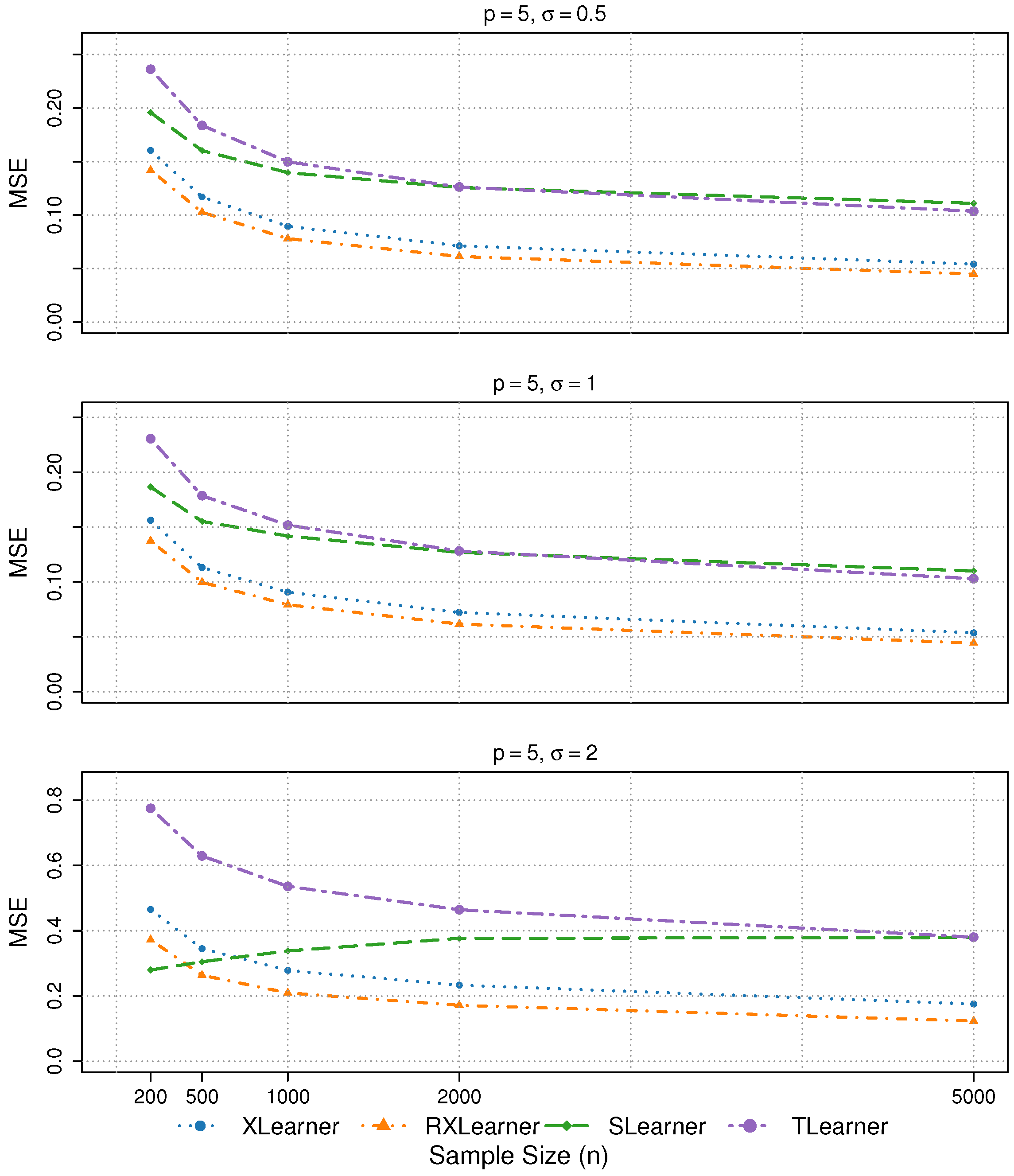
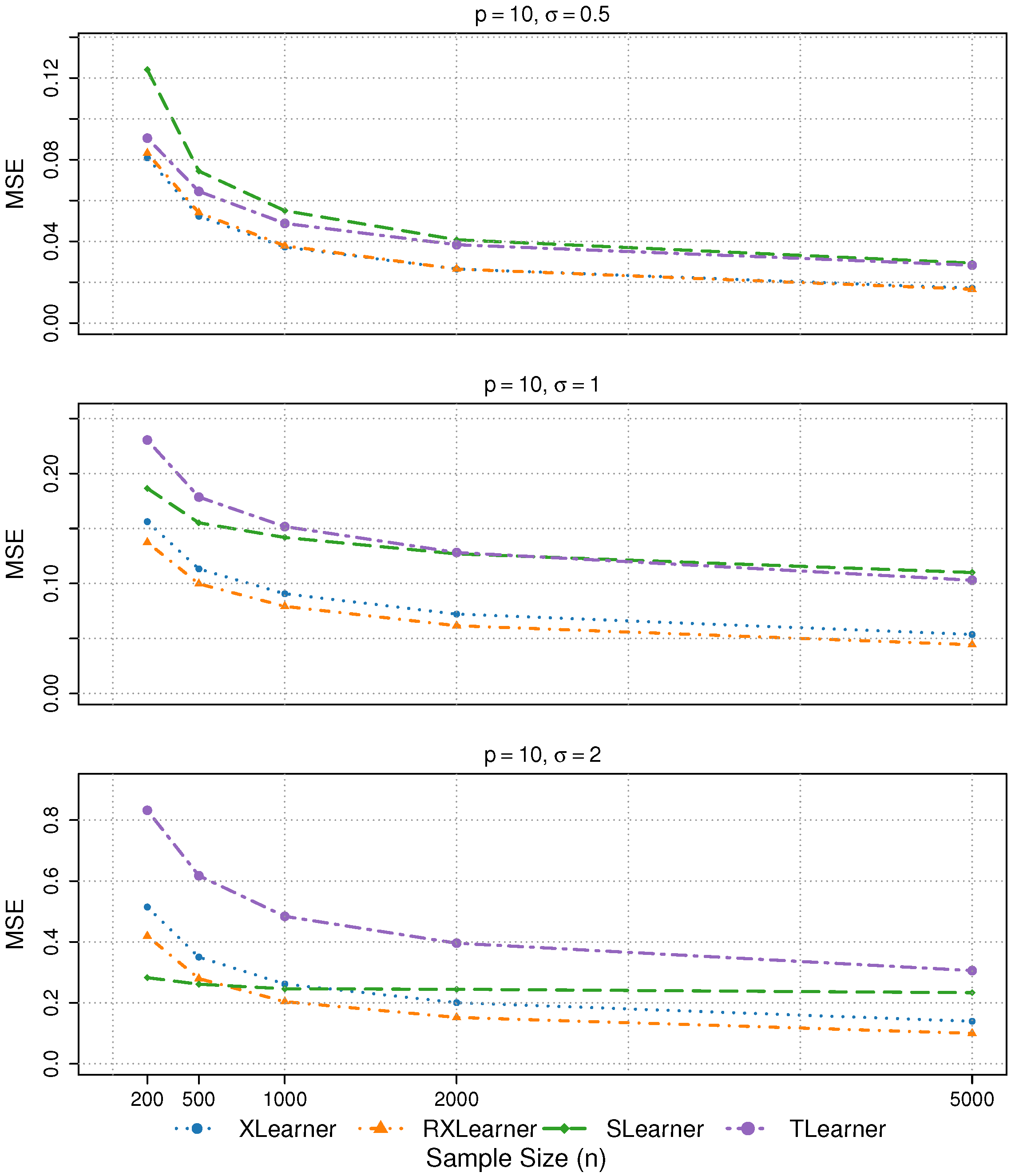
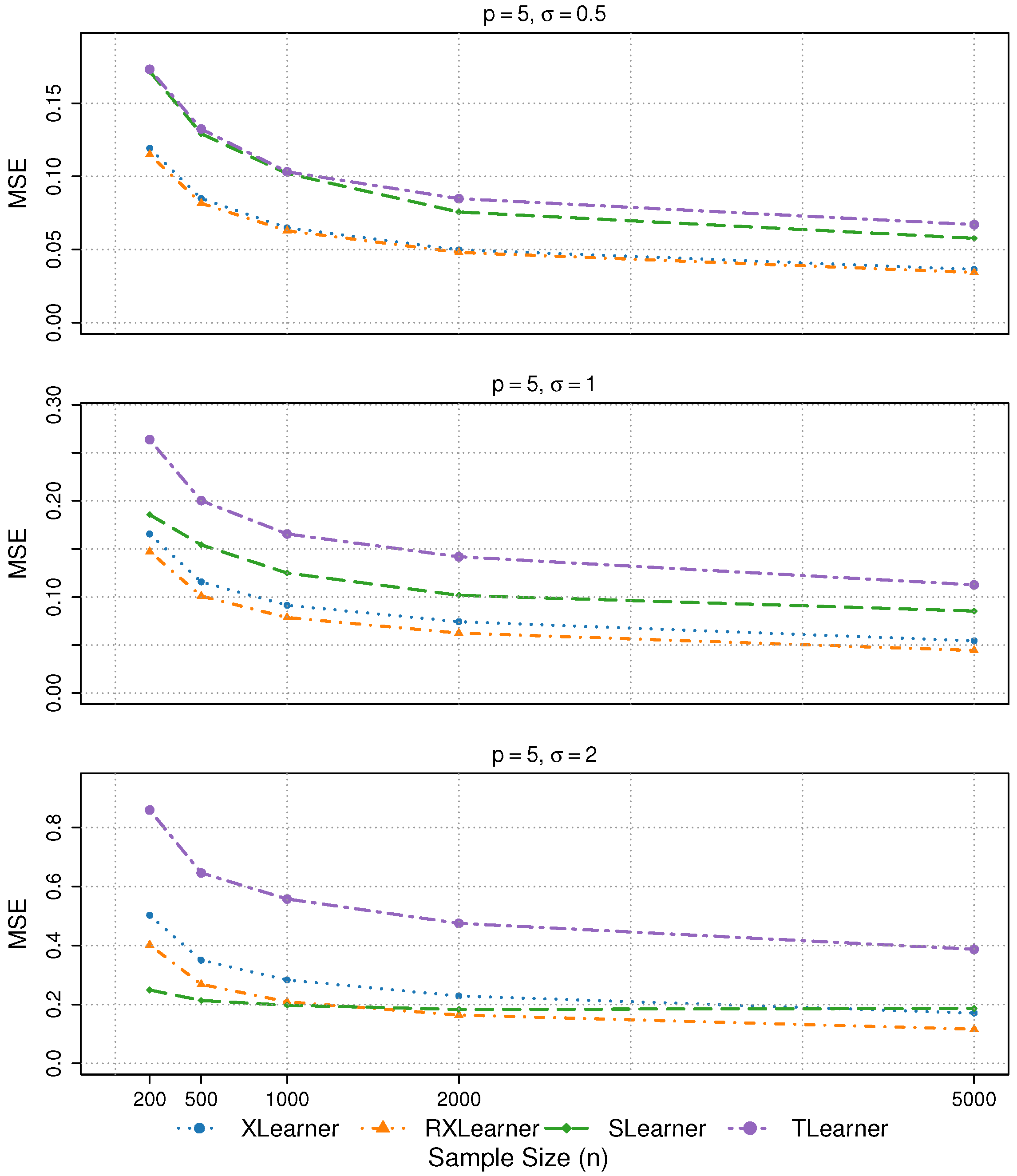
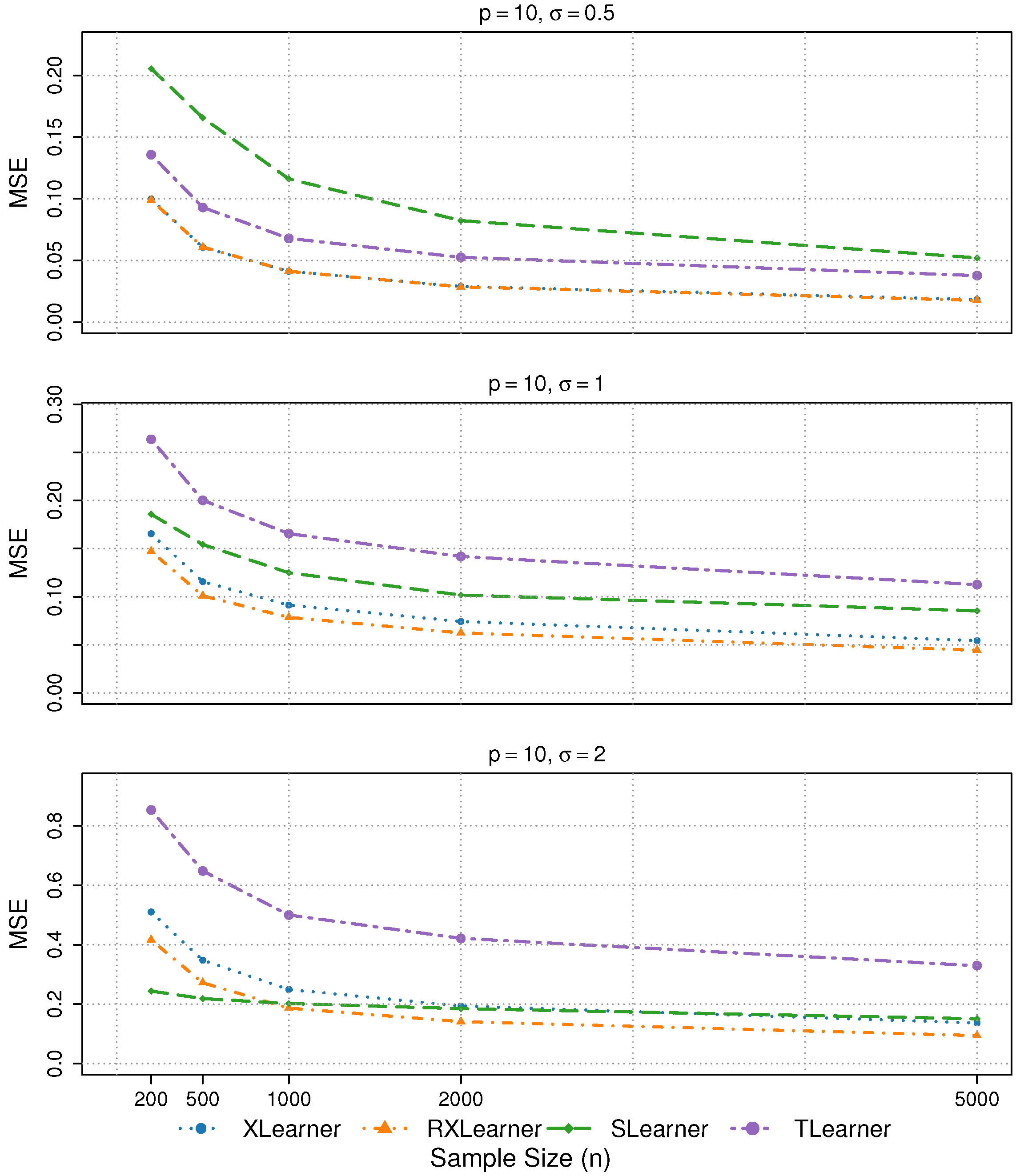
To evaluate the performance of the proposed estimator and validate the effectiveness of the theoretical framework, we first examine the performance of various estimators under different rates of change in the response function.

Simulation 1: Hölder Continuous Response Function

$${\mu }_0\left(X_i\right)=0.5{\left|X_{i4}\right|}^{{\displaystyle \frac{2}{3}}},$$

$${\mu }_1\left(X_i\right)=0.5|X_{i4}{|}^{{\displaystyle \frac{2}{3}}}+log(1+|X_{i5}\left|\right).$$

Simulation 2: Lipschitz Continuous Response Function

$${\mu }_0\left(X_i\right)=\left|X_{i5}\right|,$$

$${\mu }_1\left(X_i\right)=0.5X_{i2}+\left|X_{i5}\right|.$$

Simulation 1 reflects the Hölder continuity structure (with exponent $\alpha =2/3$), which aligns with the theoretical analysis in Section 3. We choose the form ${\mu }_0\left(x\right)=0.5{\left|X_{i4}\right|}^{2/3}$ to introduce a moderate level of nonlinearity and limited smoothness, which is representative of real-world settings where the underlying structural functions are often non-differentiable or exhibit sharp curvature changes. Such Hölder-type structures have been observed in various domains, including economics and biology (e.g., Kleiber’s law and related metabolic scaling theory; see [23]). This choice also allows us to examine the sensitivity of different estimators to non-smoothness. To further assess robustness under alternative smoothness conditions, we include a Lipschitz continuous setting in Simulation 2.

For these two types of simulations, we consider $\rho =0.5$, $e\left(x\right)=0.5$, $p\in \{5,10\}$ and $\sigma =\{0.5,1,2\}$.

4.2. Cases in Special Situations

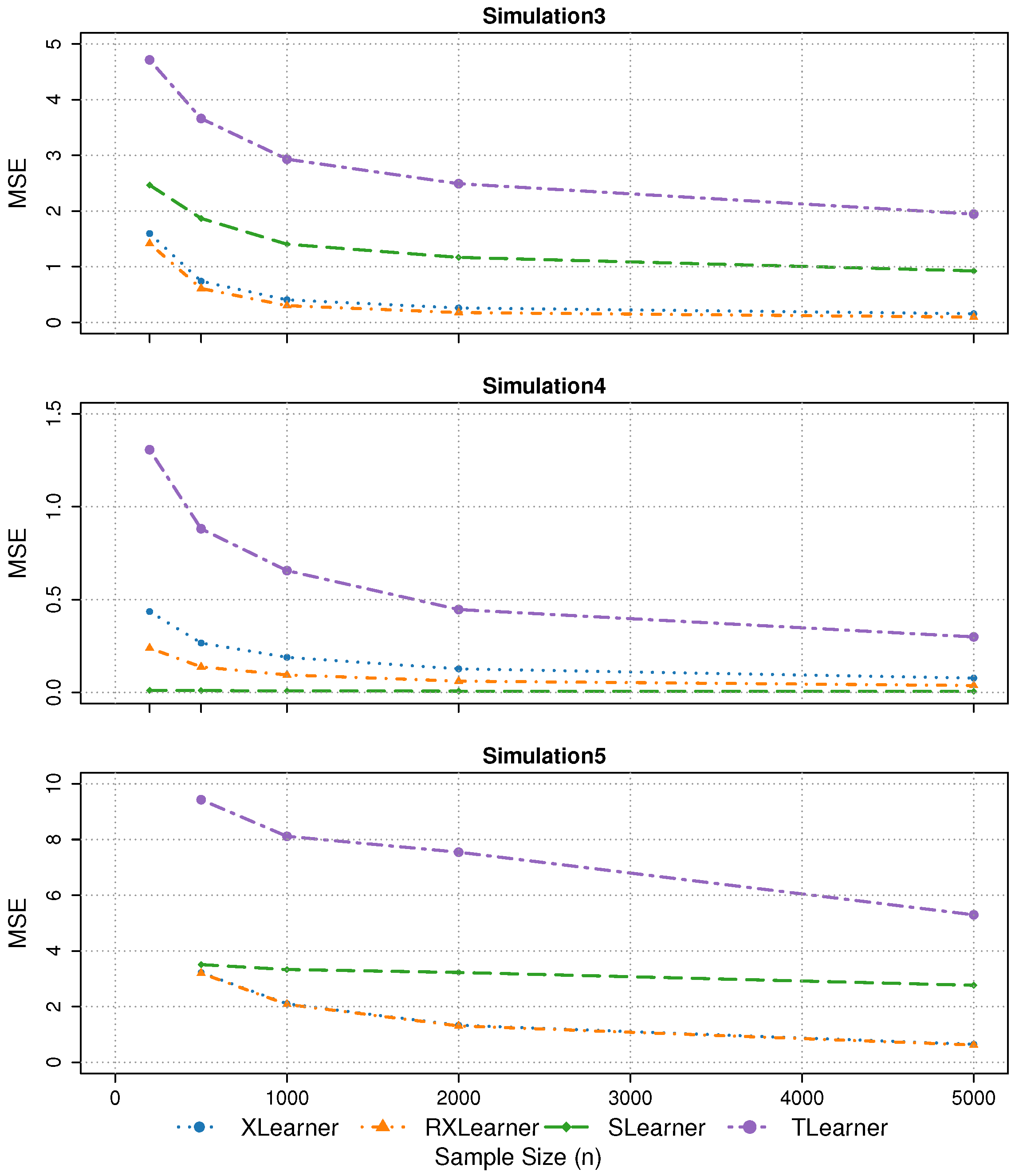
We next examine three specially designed simulation settings to evaluate the robustness and adaptability of different estimators under practically challenging conditions. These scenarios are intended to assess the performance of our proposed RXlearner when key identification assumptions are weakened. Specifically, Simulation 3 introduces confounding by violating the unconfoundedness assumption to evaluate the estimator’s robustness under model misspecification. Simulation 4 focuses on the null treatment effect case, where the true conditional treatment effect is uniformly zero across all covariate profiles, highlighting the ability of each method to avoid spurious heterogeneity. Simulation 5 investigates an extremely unbalanced treatment assignment scenario, in which the treated group constitutes a very small proportion of the sample. Given that the Xlearner is known to perform well in such settings, we aim to examine whether RXlearner can inherit or improve upon this advantage. The response function ${\mu }_0\left({\mathbf{X}}_i\right)$ in Simulation 3 is constructed following the specification of [24].

Simulation 3: Confounding

$$e_i={\displaystyle \frac{1}{1+exp(X_{i2}+X_{i3})}},$$

$${\mu }_0\left(X_i\right)=sin\left(\pi X_{i1}{X}_{i2}\right)+2{\left(X_{i3}-0.5\right)}^2+X_{i4}+0.5X_{i5},$$

$${\mu }_1\left(X_i\right)={\mu }_0\left(X_i\right)+3·I(X_{i2}>0.1).$$

We consider $\rho =0.5$, $p=10$ and $\sigma =1$.

Simulation 4: No Treatment

$${\mu }_0\left(X_i\right)=sin\left(\pi X_{i1}{X}_{i2}\right)+2{\left(X_{i3}-0.5\right)}^2+X_{i4}+0.5X_{i5},$$

$${\mu }_1\left(X_i\right)={\mu }_0\left(X_i\right).$$

We consider $\rho =0.5$, $e\left(x\right)=0.5$, $p=10$ and $\sigma =1$.

Simulation 5: Extremely Unbalanced Data

$$e_i=0.01,$$

$${\mu }_0\left(X_i\right)=sin\left(\pi X_{i1}{X}_{i2}\right)+2{\left(X_{i3}-0.5\right)}^2+X_{i4}+0.5X_{i5},$$

$${\mu }_1\left(X_i\right)={\mu }_0\left(X_i\right)+3·I(X_{i2}>0.1).$$

To evaluate the tendency of each method to spuriously detect heterogeneity when the true treatment effect is absent, we compute the false positive rate (FPR) as the proportion of units with estimated CATE values exceeding a fixed threshold $\mathrm{FPR}\left(\delta \right)={\displaystyle \frac{1}{n}}{\sum }_{i=1}^n\mathbf{1}\left(|\widehat{\tau }\left(X_i\right)|>\delta \right),$ where $\delta \in \{0.05,0.2\}$ is a pre-specified constant. These thresholds reflect varying levels of tolerance for deviations from zero. The FPR results are reported in

Table 1. False Positive Rates under Simulation 4 where the true CATE is zero.

$\mathit{\delta }$	n	False Positive Rate
		Xlearner	Slearner	Tlearner	RXlearner
0.05	200	0.927	0.553	0.957	0.906
	500	0.902	0.516	0.946	0.867
	1000	0.882	0.501	0.937	0.834
	2000	0.857	0.471	0.925	0.793
	5000	0.822	0.431	0.911	0.732
0.2	200	0.716	0.062	0.830	0.640
	500	0.626	0.049	0.786	0.509
	1000	0.557	0.034	0.752	0.416
	2000	0.478	0.024	0.709	0.315
	5000	0.378	0.016	0.658	0.201

, while the MSE results of Simulations 1–5 are presented in

Table 2. Simulation results of Simulation 1.

Simulation	p	$\mathit{\sigma }$	n	MSE
				Xlearner	Slearner	Tlearner	RXlearner
Simulation 1	5	0.5	200	0.160	0.196	0.236	0.141
			500	0.117	0.160	0.184	0.103
			1000	0.090	0.140	0.150	0.078
			2000	0.071	0.126	0.126	0.061
			5000	0.054	0.111	0.104	0.045
		1	200	0.156	0.186	0.230	0.137
			500	0.113	0.155	0.179	0.100
			1000	0.091	0.142	0.152	0.079
			2000	0.072	0.127	0.128	0.062
			5000	0.054	0.110	0.103	0.044
		2	200	0.465	0.280	0.775	0.372
			500	0.345	0.305	0.629	0.264
			1000	0.278	0.338	0.536	0.209
			2000	0.233	0.377	0.464	0.171
			5000	0.175	0.379	0.380	0.123
	10	0.5	200	0.081	0.124	0.090	0.083
			500	0.052	0.074	0.065	0.054
			1000	0.037	0.055	0.049	0.041
			2000	0.027	0.041	0.038	0.026
			5000	0.017	0.029	0.028	0.017
		1	200	0.156	0.186	0.230	0.137
			500	0.113	0.155	0.179	0.100
			1000	0.091	0.142	0.152	0.079
			2000	0.072	0.127	0.128	0.062
			5000	0.054	0.110	0.103	0.044
		2	200	0.515	0.283	0.832	0.419
			500	0.350	0.261	0.618	0.280
			1000	0.262	0.246	0.484	0.204
			2000	0.200	0.245	0.396	0.152
			5000	0.139	0.233	0.306	0.100

,

Table 3. Simulation results of Simulation 2.

Simulation	p	$\mathit{\sigma }$	n	MSE
				Xlearner	Slearner	Tlearner	RXlearner
Simulation 2	5	0.5	200	0.119	0.172	0.173	0.115
			500	0.085	0.129	0.132	0.082
			1000	0.065	0.102	0.103	0.063
			2000	0.050	0.076	0.085	0.048
			5000	0.037	0.058	0.067	0.034
		1	200	0.166	0.186	0.264	0.147
			500	0.116	0.154	0.200	0.101
			1000	0.091	0.125	0.166	0.079
			2000	0.074	0.102	0.142	0.062
			5000	0.054	0.085	0.113	0.044
		2	200	0.502	0.249	0.860	0.402
			500	0.350	0.214	0.646	0.268
			1000	0.283	0.197	0.558	0.209
			2000	0.229	0.183	0.475	0.164
			5000	0.171	0.187	0.387	0.116
	10	0.5	200	0.100	0.205	0.136	0.099
			500	0.061	0.166	0.093	0.061
			1000	0.041	0.116	0.068	0.041
			2000	0.029	0.082	0.053	0.029
			5000	0.018	0.052	0.038	0.018
		1	200	0.166	0.186	0.264	0.147
			500	0.116	0.154	0.200	0.101
			1000	0.091	0.125	0.166	0.079
			2000	0.074	0.102	0.142	0.062
			5000	0.054	0.085	0.113	0.044
		2	200	0.510	0.244	0.853	0.416
			500	0.348	0.219	0.648	0.272
			1000	0.250	0.202	0.500	0.187
			2000	0.194	0.185	0.421	0.141
			5000	0.137	0.151	0.330	0.094

and

Table 4. Simulation results of Simulations 3–5.

Simulation	n	MSE
		Xlearner	Slearner	Tlearner	RXlearner
Simulation 3	200	1.596	2.467	4.715	1.416
	500	0.741	1.868	3.662	0.610
	1000	0.406	1.405	2.931	0.302
	2000	0.261	1.169	2.492	0.178
	5000	0.157	0.926	1.946	0.096
Simulation 4	200	0.435	0.011	1.307	0.239
	500	0.266	0.010	0.882	0.137
	1000	0.189	0.008	0.656	0.094
	2000	0.127	0.007	0.446	0.061
	5000	0.077	0.005	0.299	0.037
Simulation 5	500	3.220	3.509	9.430	3.199
	1000	2.101	3.331	8.115	2.079
	2000	1.332	3.227	7.546	1.307
	5000	0.647	2.766	5.296	0.623

.

4.3. Cases with Different Correlations and Noise

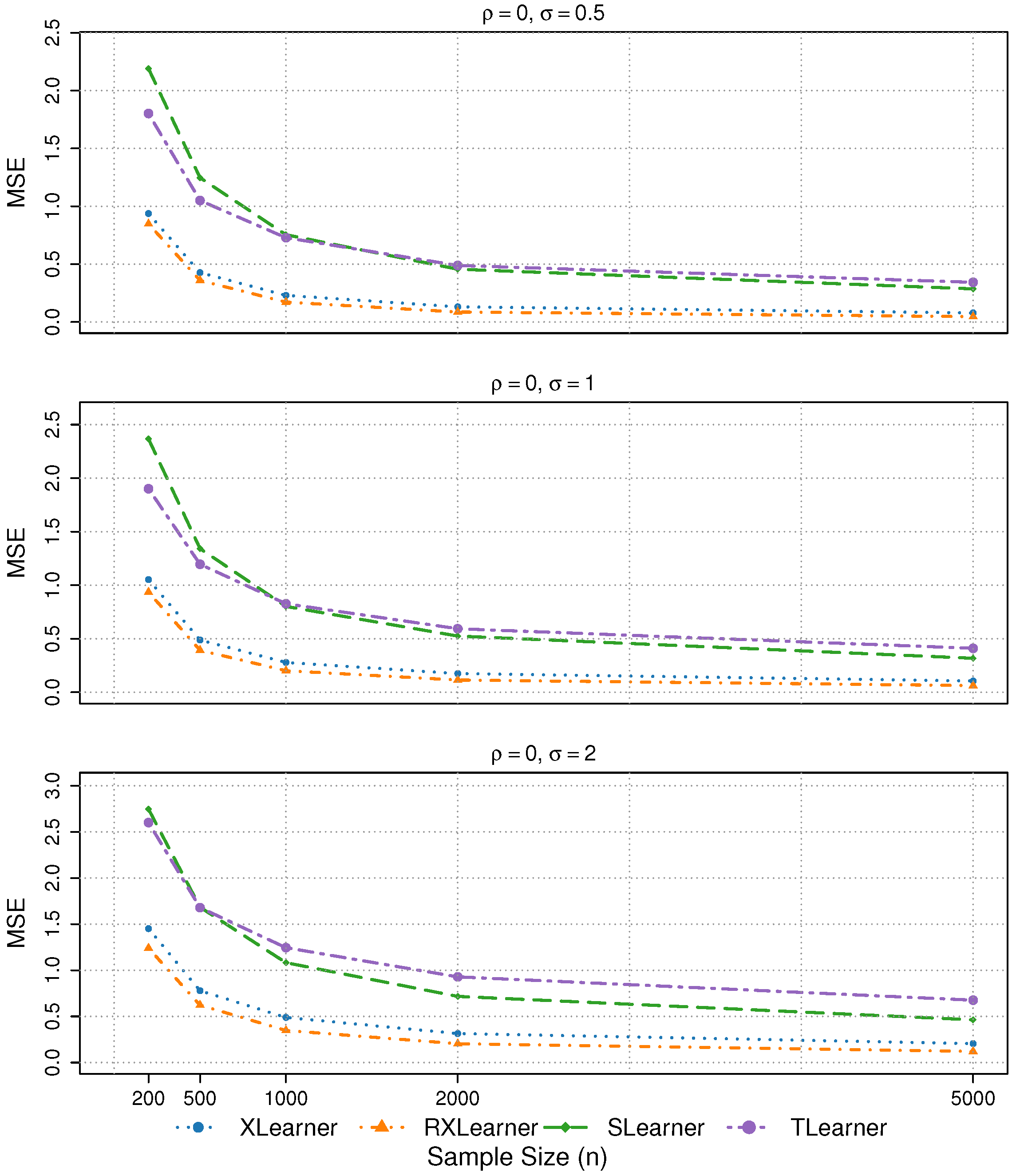
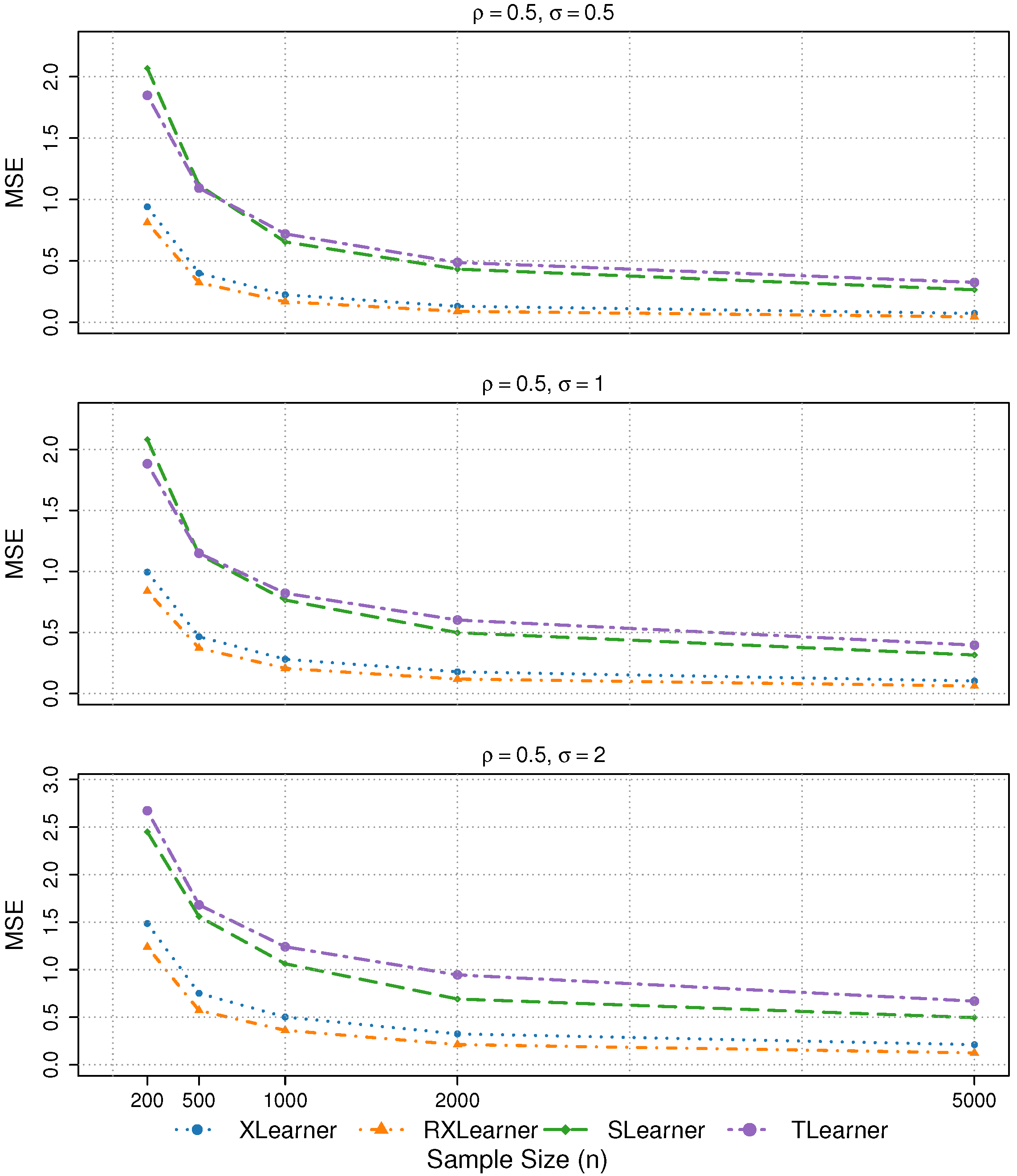
We further consider two scenarios: one concerning the impact of correlations among variables, and the other involving variations in the noise term.

Simulation 6: Different variable correlations and noise terms

$${\mu }_0\left(X_i\right)=sin\left(\pi X_{i1}{X}_{i2}\right)+2{\left(X_{i3}-0.5\right)}^2+X_{i4}+0.5X_{i5},$$

$${\mu }_1\left(X_i\right)={\mu }_0\left(X_i\right)+3·I(X_{i2}>0.1).$$

We consider $\rho \in \{0,0.5\}$, $e\left(x\right)=0.5$, $p=10$ and $\sigma \in \{0.5,1,2\}$. The corresponding MSE results are summarized in

Table 5. Simulation results of Simulation 6.

Simulation	p	$\mathit{\sigma }$	n	MSE
				Xlearner	Slearner	Tlearner	RXlearner
Simulation 6	0	0.5	200	0.937	2.190	1.802	0.848
			500	0.427	1.247	1.050	0.359
			1000	0.231	0.754	0.729	0.172
			2000	0.131	0.456	0.489	0.087
			5000	0.079	0.286	0.343	0.047
		1	200	1.052	2.367	1.901	0.935
			500	0.489	1.342	1.196	0.392
			1000	0.279	0.802	0.827	0.201
			2000	0.175	0.525	0.594	0.114
			5000	0.106	0.318	0.411	0.063
		2	200	1.451	2.746	2.600	1.240
			500	0.779	1.683	1.679	0.622
			1000	0.489	1.082	1.245	0.347
			2000	0.315	0.717	0.929	0.204
			5000	0.206	0.463	0.676	0.121
	0.5	0.5	200	0.941	2.068	1.848	0.811
			500	0.400	1.117	1.093	0.323
			1000	0.225	0.655	0.720	0.168
			2000	0.131	0.433	0.488	0.090
			5000	0.073	0.265	0.325	0.045
		1	200	0.995	2.081	1.882	0.839
			500	0.466	1.140	1.149	0.372
			1000	0.281	0.766	0.822	0.207
			2000	0.178	0.499	0.603	0.118
			5000	0.103	0.316	0.397	0.061
		2	200	1.486	2.450	2.672	1.239
			500	0.752	1.559	1.682	0.572
			1000	0.502	1.063	1.241	0.362
			2000	0.325	0.692	0.946	0.212
			5000	0.211	0.496	0.669	0.125

.

4.4. Summary of the Results

To visually compare the performances of different methods across all simulation settings, the corresponding results are presented below in Figure 1, Figure 2, Figure 3, Figure 4, Figure 5, Figure 6 and Figure 7.

Based on the simulations discussed above and the empirical results shown in the figures and tables, we summarize the key findings as follows:

1.

In Simulations 1 and 2, both the Xlearner and RXlearner outperform the Slearner and Tlearner, with RXlearner achieving the best overall performance. Simulation results consistently demonstrate the superior performance of RXlearner across various noise levels ($\sigma =0.5,1,2$), covariate dimensions ($p=5,10$), and sample sizes ($n=200$ to 5000). As the sample size increases, all methods improve, but RXlearner benefits the most, achieving the lowest MSE in nearly all settings. Its adaptive weighting mechanism proves particularly effective under high-noise and small-sample scenarios, where fixed-weight methods like Xlearner tend to suffer. Notably, RXlearner maintains strong performance even in higher dimensions, highlighting its robustness and favorable convergence behavior compared to traditional meta-learners.

2.

In Simulation 3, under confounded treatment assignment, the Tlearner exhibits the highest estimation error, followed by the Slearner. In contrast, the Xlearner and RXlearner maintain robust performance.

3.

In Simulation 4, where the treatment effect is null, the Slearner performs the best, consistent with its underlying model assumptions. Furthermore, our quantitative evaluation of the false positive rate (FPR) under this setting reveals that the Slearner maintains the lowest FPR across varying thresholds and sample sizes, followed by RXlearner, while Xlearner and Tlearner tend to produce spurious heterogeneity more frequently. This underscores the importance of cautious model selection when the true effect is absent.

4.

In Simulation 5, which involves extremely unbalanced treatment assignment, the RXlearner successfully inherits the strength of the Xlearner, while the Tlearner performs the worst due to its separate modeling for each treatment group.

5.

In Simulation 6, the four learners exhibit similar performance across different levels of variable correlation. The estimation accuracy remains stable under noise levels $\sigma =0.5$ and $\sigma =1$, with only a slight deterioration observed when $\sigma =2$.

In summary, the RXlearner consistently demonstrates the best performance across various scenarios. By enhancing the weighting mechanism of the Xlearner, RXlearner maintains equal or superior accuracy in nearly all settings.

5. Applications

To illustrate our proposed method, we analyze a large-scale Get-Out-the-Vote (GOTV) experiment, which is the same experiment used by [10] to test the Xlearner. This experiment investigates whether social pressure can be used to increase voter turnout in U.S. elections. The authors considered all voters who participated in the 2004 general election as registered voters, randomly selected a subset, and assigned them to either the treatment or control group. Households in the treatment group were sent a mailer with the message “DO YOUR CIVIC DUTY—VOTE!”, and the outcomes were observed during the 2006 primary election. We follow the method of [10] for simulation, but differ in the selection of covariates. While social pressure is typically transmitted through nearby neighbors, it is also influenced by the number of household members. Therefore, we include eight covariates, adding the number of household members as the eighth covariate, in contrast to [10], who used gender, age, and voting history in the 2000, 2002, and 2004 primary elections and the 2000 and 2002 general elections.

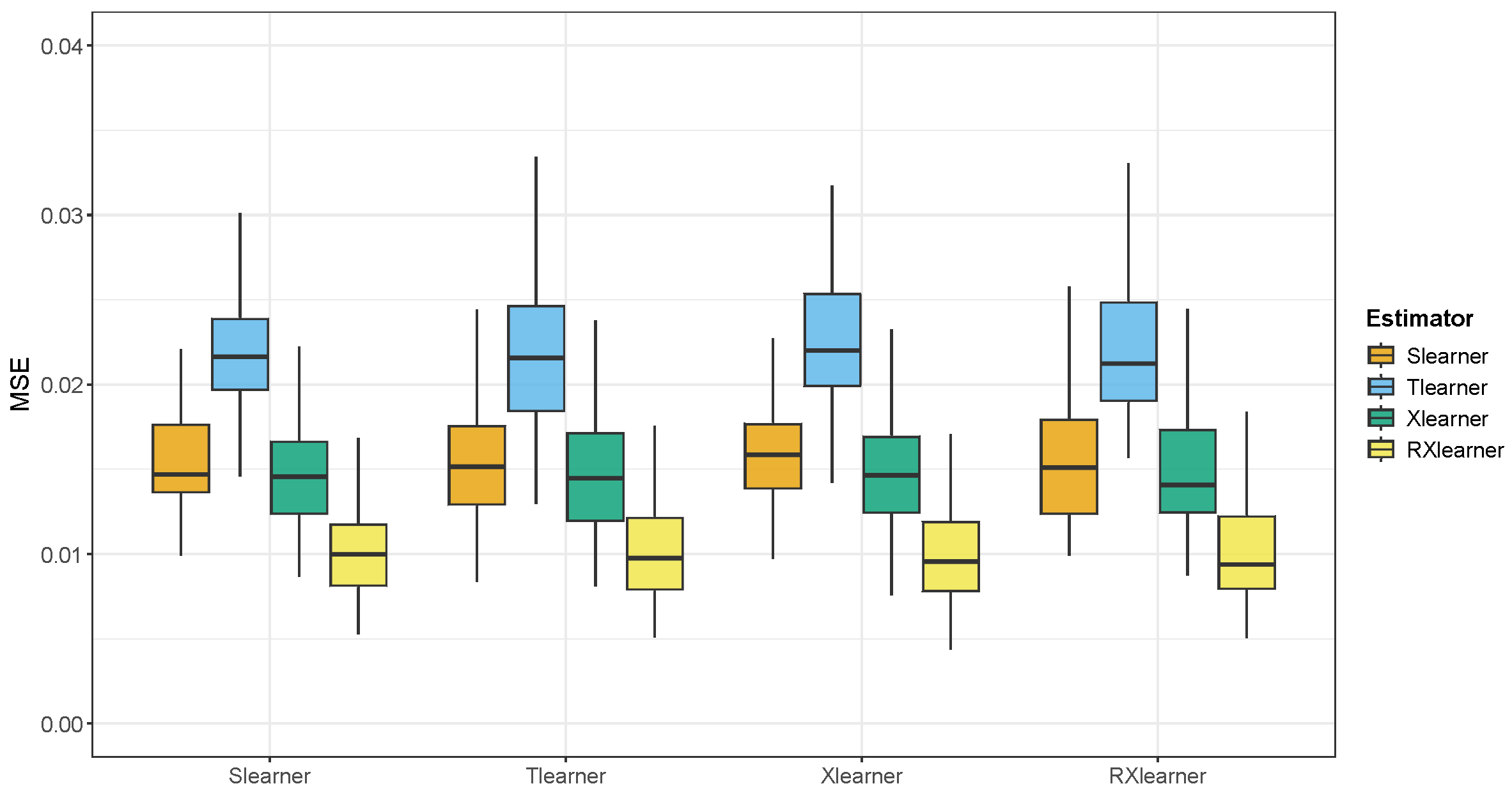
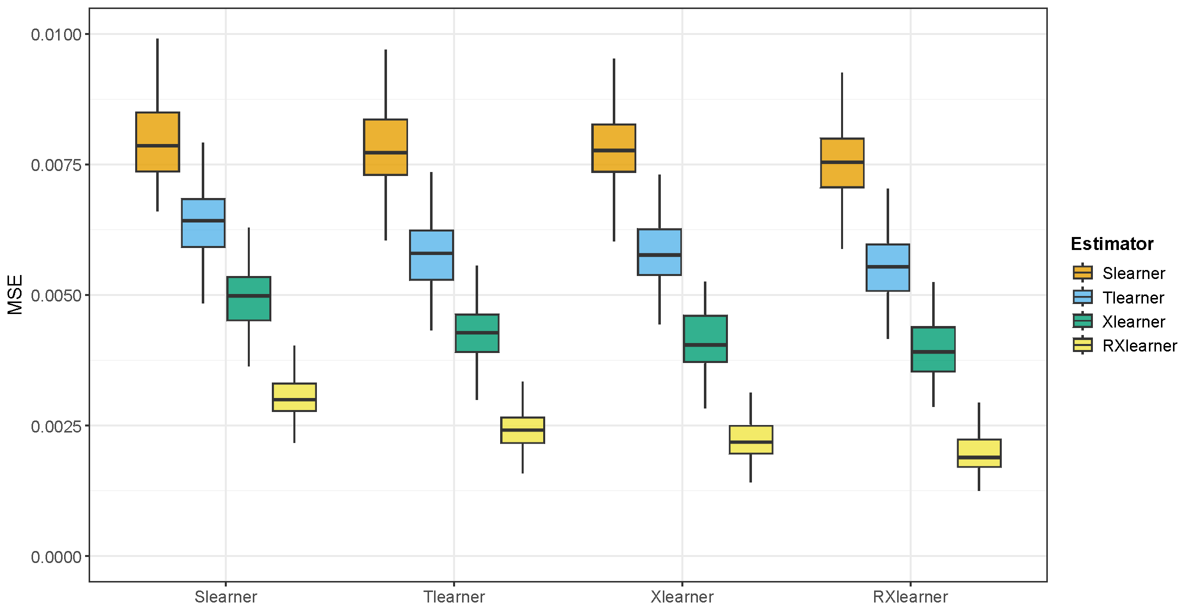
A common challenge in evaluating the accuracy of heterogeneous treatment effect estimators on real data is the lack of ground truth. To address this, we introduce synthetic treatment effects into the original dataset. We use the CATE estimates generated by the random forest-based Slearner, Tlearner, Xlearner and RXlearner as the ground truth. This allows us to assign potential outcomes to each sample and create a complete dataset. We can then verify whether different methods successfully recover the true effects and investigate whether the CATE estimates from different estimators significantly impact the results. We select 1000 and 10,000 samples from the full dataset as training sets, with the remaining data used as test sets. The proportion of treated and control groups in the selected samples matches the full dataset with $\mathbb{P}(W=1)=0.167$. Figure 8 and Figure 9 present the results of this experiment. We find that the CATE estimates from different methods have a relatively minor impact on the overall model performance. However, in smaller samples $(n=1000)$, the Slearner outperforms the Tlearner, while the opposite is true for larger samples (n = 10,000).

Notably, we observe that RXlearner achieves a significantly lower MSE compared to other methods when $n=1000$. For the other meta-learners, the performance trends are consistent with those reported in [10], where the performance gaps between methods become more pronounced in low-sample regimes. We believe that in this case, there is still room for improvement in how Xlearner selects the weighting function $g\left(x\right)$, and the optimization of $g\left(x\right)$ in RXlearner leads to a more effective combination of pseudo-responses, resulting in superior performance.

Overall, the RXlearner demonstrates significantly better performance compared to the other estimators.

6. Conclusions

This paper reviews CATE estimation methods under the meta-learner framework, including the Slearner, Tlearner, and Xlearner. Additionally, we propose a new algorithm, the RXlearner. The RXlearner retains the advantages of the Xlearner in handling unbalanced data while being more robust and effective. We conduct extensive simulation studies and real-data experiments, demonstrating that the RXlearner performs excellently in most scenarios. The error bounds of the estimator vary depending on the continuity of the response function. We establish error bounds for the case where the response function is Hölder continuous and show that using KNN as the base learner can achieve these bounds.

There are still many potential improvements for the RXlearner, such as incorporating ideas from DML by applying cross-fitting to (8) [25], or adopting a more direct approach by adding structure to (8), as explored in the works of [26,27]. Another promising direction is to incorporate regularization or complexity control into the second-stage optimization in order to further mitigate the risk of overfitting. We leave the extension of the RXlearner to future work.