The Development of Fractional Black–Scholes Model Solution Using the Daftardar-Gejji Laplace Method for Determining Rainfall Index-Based Agricultural Insurance Premiums

Abstract

The Black–Scholes model is a fundamental concept in modern financial theory. It is designed to estimate the theoretical value of derivatives, particularly option prices, by considering time and risk factors. In the context of agricultural insurance, this model can be applied to premium determination due to the similar characteristics shared with the option pricing mechanism. The primary challenge in its implementation is determining a fair premium by considering the potential financial losses due to crop failure. Therefore, this study aimed to analyze the determination of rainfall index-based agricultural insurance premiums using the standard and fractional Black–Scholes models. The results showed that a solution to the fractional model could be obtained through the Daftardar-Gejji Laplace method. The premium was subsequently calculated using the Black–Scholes model applied throughout the growing season and paid at the beginning of the season. Meanwhile, the fractional Black–Scholes model incorporated the fractional order parameter to provide greater flexibility in the premium payment mechanism. The novelty of this study was in the application of the fractional Black–Scholes model for agricultural insurance premium determination, with due consideration for the long-term effects to ensure more dynamism and flexibility. The results could serve as a reference for governments, agricultural departments, and insurance companies in designing agricultural insurance programs to mitigate risks caused by rainfall fluctuations.

1. Introduction

Individuals and companies are frequently faced with several risks and uncertainties in everyday life, which are capable of impacting their financial conditions. Investment is identified as an effective strategic method to address situations due to its ability to protect and manage financial risks [1]. Therefore, the Black–Scholes model, which was developed by Fisher Black and Myron Scholes in 1973, provides theoretical value estimates based on derivative instruments in an investment [2]. This derivative instrument is defined as a contract between two parties, and the value is derived from an underlying asset [3]. Some commonly recognized derivative products include futures, forwards, options, and others. A previous study showed the significance of the Black–Scholes model in option pricing, specifically European-style options, which could only be exercised at maturity [4]. Meanwhile, this model is not applicable for pricing American-style options that are exercisable at any time before maturity. The Black–Scholes model remains a fundamental basis for different advancements in financial theory and practice, despite its limitations.

The standard Black–Scholes model has been developed over the time into the fractional Black–Scholes model, with the inclusion of the Hurst parameter [5]. This was achieved by fractionalizing the maturity time to ensure a more comprehensive analysis of asset price dynamics [6,7,8]. The inclusion of the Hurst parameter is significant due to its ability to handle data with long-term dependence, which leads to more relevance in financial analysis, particularly in volatile market conditions [9,10]. Furthermore, the fractional Black–Scholes model provides a more flexible method in describing the behavior of assets and risks, which expands the scope of application to a wide range of financial instruments. Several methods can be used to obtain solutions for the fractional Black–Scholes model, including the Sumudu transform [11,12], Laplace transform [13,14], Kamal transform [15], Adomian decomposition method [16], differential transformation method [17], and others.

Several other methods have been continuously developed to find solutions. An example is the Daftardar-Gejji method, which is an extension of the Adomian decomposition. The advantage is that it does not require the prior formation of Adomian polynomials. The Daftardar-Gejji method has been applied in different studies, including the determination of a solution to the Multispecies Lotka–Volterra equation by Batiha et al. [18]. It has also been proven to be effective and straightforward in solving the fractional Black–Scholes model [19]. Moreover, the method can be combined with the Laplace transform to improve the accuracy and stability of the solution. The Laplace transform scheme based on the Daftardar-Gejji method allows for obtaining approximation solutions for nonlinear differential equations more systematically. The main idea is to decompose the solution into an infinite series and apply the Laplace transform to the differential equation. The advantage is in the rapid convergence of the solution sequence to the exact solution [20]. Therefore, this study adopted a combined method known as the Daftardar-Gejji Laplace method to obtain a more accurate solution for the fractional Black–Scholes model.

The standard and fractional Black–Scholes models are important in the field of economics and have significant contributions in agricultural insurance. This is due to the similar characteristics between the option pricing mechanism and agricultural insurance premiums, particularly in terms of risk and uncertainty [21]. The agricultural sector faces a high level of risk associated with crop failure, which can result in financial losses and decreased production. Part of the main factors causing these risks are climate change, particularly rainfall fluctuations. Therefore, effective risk mitigation strategies, including traditional protection and agricultural insurance schemes, are needed to protect farmers from such financial risks [22]. The traditional protection is generally implemented through government budget allocations to address the impacts of natural disasters [23]. However, this method has limitations, particularly based on the availability of economically viable insurance in each country. This shows the need to design an alternative mechanism through agricultural insurance schemes in order to provide more sustainable financial protection for farmers.

Agricultural insurance has experienced growth, as observed in different schemes developed based on claim limitations, such as crop failure-based, yield-based, and climate index-based insurance. The application of climate index-based agricultural insurance using rainfall as a parameter is considered an effective solution to protect farmers from the risk of crop failure caused by rainfall variability [24]. This insurance system emphasizes rainfall as the basis for determining claims or compensation payments. Farmers can receive compensation from an insurance company when an extreme, unexpected rainfall condition occurs [25]. In return, farmers are required to pay premiums in the form of money, which serves as a contribution to participation in the insurance program [26]. In rainfall index-based agricultural insurance, the premium is paid each growing season and is determined based on the variability in rainfall as the primary risk indicator.

The concept of premium determination in agricultural insurance is similar to option pricing in financial markets. For example, a put option holds value when the market price is lower than the strike price and becomes worthless when the market price is higher. This concept is analogous to the premium determination in rainfall index-based agricultural insurance, where the market price is represented by the average total rainfall over recent years, and the strike price corresponds to the predetermined rainfall trigger index based on percentiles. This shows that farmers receive compensation when the latest rainfall index falls below the agreed-upon trigger index, because the insured risk is flood. Conversely, no compensation is provided when the rainfall index exceeds the trigger level [21]. This shows that the standard and fractional Black–Scholes models can be used in determining both premiums and compensation in rainfall index-based agricultural insurance.

A previous study by Chicaiza and Cabedo applied the Black–Scholes model in insurance and finance to determine insurance premiums for high-cost diseases in Colombia [27]. The results showed that the premium price determined did not significantly differ from the value calculated using actuarial analysis. Weber et al. [28] also studied the design of rainfall index-based agricultural insurance in Tajikistan to protect income losses caused by weather in cotton production. The results showed that index-based agricultural insurance was significant in overcoming potential losses in the cotton sector. Moreover, Filiapuspa et al. [29] focused on premium determination for rainfall index-based agricultural insurance for rice commodities in Banten Province by applying the Black–Scholes model. The results found that greater rainfall led to an increase in the premium to be paid. Paramita et al. [30] also calculated pure premiums for weather-based insurance for farmers in Wonogiri, Central Java, using the Black–Scholes model. The results showed that farmers could file a claim and receive compensation of IDR 13,600,000 when rainfall was below 100 mm/month.

The trend from the previous studies showed several limitations in the method of determining premiums for rainfall index-based agricultural insurance. This was because most studies used the Black–Scholes model with a focus on drought risk. The gaps identified led to the application of the fractional Black–Scholes model in this study to determine premiums for rainfall index-based agricultural insurance, covering both drought and flood risks. Moreover, fractional Black–Scholes solutions were obtained using a combination method called the Daftardar-Gejji Laplace method. The results were expected to produce premiums considered more diverse by considering long-term effects in order to provide flexibility in the payment mechanism. This study contributes by providing new insights for insurance companies in determining premiums and indemnities in rainfall index-based agricultural insurance. It can also serve as a reference for governments and agriculture departments in formulating policies and designing socialization programs for farmers participating in agricultural insurance.

This article is structured as follows: Section 2 introduces the standard Black–Scholes model and the fractional extension as the theoretical foundation of this study. Building upon this framework, Section 3 conducts a Lie symmetry analysis of the fractional Black–Scholes partial differential equation to understand the underlying mathematical structure. Section 4 provides an explicit solution to the fractional Black–Scholes model using the Daftardar-Gejji Laplace method, providing a systematic method for the solution. Section 5 proceeds with the identification of long-term effects and the estimation of the fractional order parameter to enhance the accuracy of the model. Section 6 outlines the object of study, the data used, as well as the tools and methods used for data processing. These methods are later applied to the computation of agricultural insurance premiums based on the rainfall index and the corresponding insurance payouts in Section 7. The results are further analyzed in Section 8 to assess the performance and practical relevance of the proposed model. Finally, Section 9 summarizes the key results and offers concluding remarks along with directions for future study.

2. The Standard and Fractional Black–Scholes Models

The Black–Scholes model was first introduced by Fisher Black and Myron Scholes in 1973 as a significant breakthrough in the field of financial derivatives. It was developed in the form of a partial differential equation using a continuous-time method. Subsequently, Robert C. Merton expanded its application in option pricing, and it became known as the Black–Scholes model. According to Luenberger [31], an option is an agreement or contract that grants the holder the right but not the obligation to buy or sell a specific asset at a predetermined price and time. Options are further classified into American and European types, based on the execution time, as well as the call and put based on the function [4]. The following assumptions were used in determining option prices based on the Black–Scholes model [32,33]:

(1)

The option under consideration is a European option, which can only be exercised at maturity.

(2)

Stock prices follow a stochastic process with a lognormal distribution, assuming a constant variance in stock returns.

(3)

The risk-free interest rate is constant.

(4)

There is no dividend payment on the stock during the option term.

(5)

There are no taxes or transaction costs in the process of buying or selling options.

In the application of the Black–Scholes model for option pricing, it is assumed that stock price movements follow a geometric Brownian motion. The process leads to the following stock price dynamics:

$$dS=\mu Sdt+\sigma SdB$$

(1)

where $B$ represents a standard Brownian motion. Let $V(S,t)$ denote the option price at time $t$ for a stock price $S$. Applying Itô’s lemma produces the following:

$$dV=\left({\displaystyle \frac{\partial V}{\partial t}}+\mu S{\displaystyle \frac{\partial V}{\partial S}}+{\displaystyle \frac{1}{2}}{\sigma }^2{S}^2{\displaystyle \frac{{\partial }^{2}V}{\partial S^2}}\right)dt+\sigma S{\displaystyle \frac{\partial V}{\partial S}}dB.$$

(2)

The discretized form of the process and results are presented as follows:

$$∆S=\mu S∆t+\sigma S∆B$$

(3)

$$∆V=\left({\displaystyle \frac{\partial V}{\partial t}}+\mu S{\displaystyle \frac{\partial V}{\partial S}}+{\displaystyle \frac{1}{2}}{\sigma }^2{S}^2{\displaystyle \frac{{\partial }^{2}V}{\partial S^2}}\right)∆t+\sigma S{\displaystyle \frac{\partial V}{\partial S}}∆B$$

(4)

where $∆S$ and $∆V$ represent the changes in $S$ and $V$ over a small time interval $∆t$. The Itô’s lemma shows that the underlying Wiener process for both $S$ and $V$ is the same. This shows that the term $∆B(=ϵ\sqrt{∆t})$ appearing in Equations (3) and (4) refers to the same stochastic process. Therefore, a portfolio consisting of the underlying stock and its derivative can be constructed to ensure the Wiener process is eliminated. The portfolio comprises a position of $-1$: derivative and $+{\displaystyle \frac{\partial V}{\partial S}}$: stock. The trend shows that the holder of the portfolio takes a short position in one derivative and a long position in ${\displaystyle \frac{\partial V}{\partial S}}$ stocks. Under this strategy, the portfolio value is presented as follows:

$$\Pi =-V+{\displaystyle \frac{\partial V}{\partial S}}S.$$

(5)

Over a small time interval $∆t$, the change in the option value is

$$∆\Pi =-∆V+{\displaystyle \frac{\partial V}{\partial S}}∆S.$$

(6)

By substituting Equations (3) and (4) into Equation (6), the expression produced for $d\Pi$ is

$$d\Pi =\left(-{\displaystyle \frac{\partial V}{\partial t}}-{\displaystyle \frac{1}{2}}{\displaystyle \frac{{\partial }^{2}V}{\partial S^2}}{\sigma }^2{S}^2\right)dt.$$

(7)

Based on Equation (7), the portfolio does not contain the stochastic Brownian motion term $∆B$. Therefore, assuming no arbitrage, the portfolio $\Pi$ is required to be risk-free over the small time interval $∆t$. The assumption implies that the portfolio needs to earn the same return as other short-term risk-free securities. This leads to the no-arbitrage condition, which requires introducing the portfolio according to

$$d\Pi =r\Pi dt.$$

(8)

By substituting Equations (5) and (7) into Equation (8), the following relationship is produced:

$$\left(-{\displaystyle \frac{\partial V}{\partial t}}-{\displaystyle \frac{1}{2}}{\displaystyle \frac{{\partial }^{2}V}{\partial S^2}}{\sigma }^2{S}^2\right)dt=r\left(-V+{\displaystyle \frac{\partial V}{\partial S}}S\right)dt.$$

(9)

This leads to the Black–Scholes partial differential equation for option pricing:

$${\displaystyle \frac{\partial V}{\partial t}}+{\displaystyle \frac{1}{2}}{\displaystyle \frac{{\partial }^{2}V}{\partial S^2}}{\sigma }^2{S}^2+rS{\displaystyle \frac{\partial V}{\partial S}}-rV=0.$$

(10)

For a European call option $C(S,t)$, the Black–Scholes differential equation becomes as follows:

$${\displaystyle \frac{\partial C}{\partial t}}+{\displaystyle \frac{1}{2}}{\displaystyle \frac{{\partial }^{2}C}{\partial S^2}}{\sigma }^2{S}^2+rS{\displaystyle \frac{\partial C}{\partial S}}-rC=0$$

(11)

with the boundary conditions $C(0,t)=0, C(S,t)=S$ for $S\to \infty$, and $C(S,T)=\mathrm{m}\mathrm{a}\mathrm{x}\{S-E,0\}$, where $\sigma$ is the volatility of the underlying asset, $E$ is the exercise price, $t$ represents the time to maturity, and $r$ is the risk-free interest rate. Using the change in variables $S=E{e}^x, t=T-{\displaystyle \frac{2\tau }{{\sigma }^2}}, C(S,t)=Ev(x,t)$, and $k={\displaystyle \frac{2\tau }{{\sigma }^2}}$, Equation (11) can be transformed into the following simplified form:

$${\displaystyle \frac{\partial v}{\partial \tau }}={\displaystyle \frac{{\partial }^{2}v}{\partial x^2}}+(k-1){\displaystyle \frac{\partial v}{\partial x}}-rv$$

(12)

with the initial condition $V(x,0)=\mathrm{m}\mathrm{a}\mathrm{x}\{e^x-\mathrm{1,0}\}$.

According to Hull [34], the European-type Black–Scholes model for determining the price of a call option is presented in Equation (13), while the price of a put option is shown in Equation (14).

$$C_B=S_{0}N\left(d_1\right)-K{e}^{-rt}N\left(d_2\right)$$

(13)

$$P_B=K{e}^{-rt}N\left(-d_2\right)-S_{0}N\left({-d}_1\right)$$

(14)

where the cumulative distributions $d_1$ and $d_2$ are presented in Equations (15) and (16) as follows:

$$d_1={\displaystyle \frac{\mathit{ln}\left(\frac{S_0}{K}\right)+\left(r+\frac{{\sigma }^2}{2}\right)t}{\sigma \sqrt{t}}}$$

(15)

$$d_2={\displaystyle \frac{\mathit{ln}\left(\frac{S_0}{K}\right)+\left(r-\frac{{\sigma }^2}{2}\right)t}{\sigma \sqrt{t}}}=d_1-\sigma \sqrt{t}$$

(16)

$C_B$ is the price of the Black–Scholes European call option, $P_B$ is the price of the Black–Scholes European put option,$S_0$ is the initial stock price, $S_T$ is the stock price at maturity, $K$ is the strike price, $r$ is the risk-free interest rate, $t$ is the time at maturity, $\sigma$ is the standard deviation of stock price, and $N\left(x\right)$ is the cumulative distribution function of the standard normal distribution.

The standard Black–Scholes model presents several limitations, including the necessity for practitioners to frequently adjust the volatility parameter in order to reflect current market information. It also does not account for the presence of long-range dependence in asset returns [35]. The efforts to address the limitations require alternative modeling methods. In the evolution of modern financial markets, fractional Brownian motion has gained significant attention due to its ability to capture long-term dependence structures [36]. Consequently, the application of the fractional Black–Scholes model for option pricing has become increasingly relevant. The framework assumes that stock prices follow the fractional Brownian motion and leads to the production of the following stock price dynamics:

$$dS=\mu Sdt+\sigma S\diamond d{B}_H$$

(17)

where $B_H$ denotes the fractional Brownian motion and $\diamond$ represents the Wick product. However, the use of the Wick product requires particular attention to several theoretical and practical aspects [37]. It is specifically not equivalent to the conventional pointwise multiplication, which introduces challenges in economic interpretation. Furthermore, pricing formulations based on Wick calculus typically do not offer a framework for replication strategies. This shows the possibility of not working in line with the risk-neutral valuation principles that underlie arbitrage models. Moreover, the implementation of Wick-based models remains limited within financial markets.

Despite the concerns identified, the properties of self-similarity and long-range dependence make fractional Brownian motion a suitable tool for different applications, including mathematical finance. However, the conventional stochastic calculus cannot be applied for its analysis, because $H\ne {\displaystyle \frac{1}{2}}$, and fractional Brownian motion is neither a Markov process nor a semi-martingale. Financial models driven by $B_H$ can also lead to arbitrage opportunities. The development of a new type of integral based on the Wick product (see [38,39]), known as the fractional Itô integral, shows that the corresponding fractional Black–Scholes model of the Itô type does not admit arbitrage. According to Necula [40], the option price $V(S,t)$ is required to satisfy the following fractional Black–Scholes partial differential equation:

$${\displaystyle \frac{\partial V}{\partial t}}+\delta t^{2\delta -1}{\displaystyle \frac{{\partial }^{2}V}{\partial S^2}}{\sigma }^2{S}^2+rS{\displaystyle \frac{\partial V}{\partial S}}-rV=0$$

(18)

where $\delta$ represents the fractional order parameter, with $0<\delta \le 1$, and the initial condition is given by $V(x,0)=\mathrm{m}\mathrm{a}\mathrm{x}\{e^x-\mathrm{1,0}\}$. Furthermore, Necula [40] derived the fractional Black–Scholes model for European-type call option pricing through Equation (19) and the put option pricing formula in Equation (20).

$$C_{BF}=S_{0}N\left(d_1\right)-K{e}^{-rt}N\left(d_2\right)$$

(19)

$$P_{BF}=K{e}^{-rt}N\left(-d_2\right)-S_{0}N\left({-d}_1\right)$$

(20)

where the cumulative distributions $d_1$ and $d_2$ are presented in Equations (21) and (22) as follows:

$$d_1={\displaystyle \frac{\mathit{ln}\left(\frac{S_0}{K}\right)+rt+\frac{1}{2}{\sigma }^2{t}^{2\delta }}{\sigma \sqrt{t^{2\delta }}}}$$

(21)

$$d_2={\displaystyle \frac{\mathit{ln}\left(\frac{S_0}{K}\right)+rt-\frac{1}{2}{\sigma }^2{t}^{2\delta }}{\sigma \sqrt{t^{2\delta }}}}$$

(22)

$C_{BF}$ is the price of the fractional Black–Scholes European call option, $P_{BF}$ is the price of the fractional Black–Scholes European put option, and $\delta$ is the fractional order parameter.

3. Lie Symmetry Analysis of the Fractional Black–Scholes Partial Differential Equation

The Lie symmetry analysis method was developed by the Norwegian mathematician Sophus Lie in the late nineteenth century. As a modern method among several analytical methods, Lie symmetry analysis has been effectively adopted in a wide range of fractional differential equation models across different fields of applied science (see [41,42,43]). In this study, it was extended to the fractional Black–Scholes partial differential equation as follows:

$${\displaystyle \frac{{\partial }^{\delta }V}{\partial t^{\delta }}}+{\displaystyle \frac{1}{2}}{\displaystyle \frac{{\partial }^{2}V}{\partial S^2}}{\sigma }^2{S}^2+rS{\displaystyle \frac{\partial V}{\partial S}}-rV=0$$

(23)

where $0<\delta \le 1$, $V(S,t)$ is the option price at time $t$ for stock price $S$, $r$ is the risk-free interest rate, and $\sigma$ is the standard deviation of the stock price [11]. The invariance condition of the Equation (23) is

$${\eta }^{\delta ,t}+{\displaystyle \frac{1}{2}}{\eta }^{SS}{\sigma }^2{S}^2+{\sigma }^{2}S\xi V_{SS}+rS{\eta }^S+r\xi V_S-r\eta =0.$$

(24)

By substituting the derivatives ${\eta }^S$, ${\eta }^{SS}$, and ${\eta }^{\delta ,t}$ obtained from [44,45], the determining equations for the symmetry group are obtained as follows:

$$\begin{array}{r}{\displaystyle \frac{1}{2}}{\sigma }^2{S}^2({\eta }_V-2{\xi }_S)-{\displaystyle \frac{1}{2}}{\sigma }^2{S}^2({\eta }_V-\delta D_t(\tau ))+{\sigma }^{2}S\xi =0\\ {\sigma }^2{S}^2{\eta }_{SV}-{\displaystyle \frac{1}{2}}{\sigma }^2{S}^2{\xi }_{SS}-rS({\eta }_V-\delta D_t(\tau ))+rS({\eta }_V-{\xi }_S)+r\xi =0\\ {\tau }_S={\tau }_V={\xi }_V={\xi }_t=0\\ {\displaystyle \frac{{\partial }^{\delta }\eta }{\partial t^{\delta }}}-V{\displaystyle \frac{{\partial }^{\delta }{\eta }_V}{\partial t^{\delta }}}+{\displaystyle \frac{1}{2}}{\sigma }^2{S}^2{\eta }_{SS}+rS{\eta }_S+r({\eta }_V-\delta D_t(\tau ))V-r\eta =0\\ \left(\begin{array}{c}\delta \\ n\end{array}\right){\displaystyle \frac{{\partial }^n{\eta }_V}{\partial t^n}}-\left(\begin{array}{c}\delta \\ n+1\end{array}\right)D_t^{n+1}(\tau )=0.\end{array}$$

(25)

The determining equations can be integrated to produce the following general solution:

$$\begin{array}{l}\eta =\left[{\displaystyle \frac{a_1\delta }{2{\sigma }^2}}\left({\displaystyle \frac{1}{2}}{\sigma }^2-D\right)\mathrm{l}\mathrm{n}(S)+a_2\right]+v(t,S)\\ \xi ={\displaystyle \frac{1}{2}}{a}_1\delta S\mathrm{l}\mathrm{n}(S)+a_{3}S\\ \tau =a_{1}t+a_4\end{array}$$

(26)

where, $a_1,a_2,a_3,$ and $a_4$ are arbitrary constants, $D=r-{\sigma }^2/2\ne 0$, and $v(t,S)$ is any solution of the fractional Black–Scholes equation. The variable transformation is required to preserve the structure of the fractional derivative operator, leading to the following invariance condition:

$$\tau (t,S,V){|}_{t=0}=0$$

(27)

The trend shows that $\tau =a_{1}t$ and the symmetry group of the fractional Black–Scholes equation is spanned by the vector fields

$$\begin{gathered} { X}_1=t{\displaystyle \frac{\partial }{\partial t}}+{\displaystyle \frac{1}{2}}\delta Sln(S){\displaystyle \frac{\partial }{\partial S}}+{\displaystyle \frac{\delta }{2{\sigma }^2}}\left({\displaystyle \frac{1}{2}}{\sigma }^2-D\right)V\mathrm{l}\mathrm{n}(S){\displaystyle \frac{\partial }{\partial V}},X_2=S{\displaystyle \frac{\partial }{\partial S}}, \\ {X}_3=V{\displaystyle \frac{\partial }{\partial V}}, X_{\infty }=v(t,S){\displaystyle \frac{\partial }{\partial V}}. \end{gathered}$$

(28)

4. Solution of the Fractional Black–Scholes Model Using the Daftardar-Gejji Laplace Method

This section discusses the Daftardar-Gejji method and Laplace transform, which are later combined to determine the solution to the fractional Black–Scholes model. The Daftardar-Gejji method is an extension of the Adomian decomposition with the advantage of not requiring the prior formation of polynomials [46]. According to Batiha et al. [18], this method uses an operator equation and is presented as follows:

$$u=f+L(u)+N(u)$$

(29)

where $L$ is a linear invertible operator, $N$ is a nonlinear operator, and $f$ is a given function. It is assumed that the function $u$ can be decomposed into an infinite series, as defined in Equation (30).

$$u=\sum _{n=0}^{\infty }{u}_n$$

(30)

such that the linear operator $L(u)$ becomes as follows:

$$L(u)=L\left(\sum _{n=0}^{\infty }{u}_n\right)=\sum _{n=0}^{\infty }{L(u}_n).$$

(31)

The nonlinear operator $N(u)$ can be decomposed as presented in Equation (32).

$$N(u)=N\left(\sum _{n=0}^{\infty }{u}_n\right)=N(u_0)+\sum _{n=1}^{\infty }\left\{N\left(\sum _{j=0}^n{u}_j\right)-N\left(\sum _{j=0}^{n-1}{u}_j\right)\right\}=\sum _{n=0}^{\infty }{G}_n$$

(32)

where $G_0=N(u_0)$ and the equation becomes as follows:

$$G_n=\left\{N\left(\sum _{j=0}^n{u}_j\right)-N\left(\sum _{j=0}^{n-1}{u}_j\right)\right\},\hspace{1em}\hspace{1em}n\ge 1.$$

(33)

The following relationship was obtained by substituting Equations (30)–(32) into Equation (29):

$$\sum _{n=0}^{\infty }{u}_n=f+\sum _{n=0}^{\infty }{L(u}_n)+\sum _{n=0}^{\infty }{G}_n.$$

(34)

In general, the recursive relation is provided as follows:

$$u_0=f$$

$$u_{n+1}=L\left(u_n\right)+G_n,\hspace{1em}\hspace{1em}n=0, 1, 2,\dots$$

The Laplace transform is a class of integral transformations used to convert ordinary differential equations into algebraic equations and partial differential equations into ordinary differential equations. The Laplace transform can be used to determine the solution of differential equations through the transformation into algebraic equations.

Definition 1

([47]). Let $f(t)$ be a real- or complex-valued function defined for $t>0$ , and let $s$ be a real or complex parameter. The Laplace transform of $f(t)$ is given by the following:

$$\mathcal{L}\left\{f\left(t\right)\right\}=F\left(s\right)=\underset{0}{\overset{\infty }{\int }}f(t)e^{-st}dt=\underset{a\to \infty }{\mathit{lim}}\underset{0}{\overset{a}{\int }}f(t)e^{-st}dt$$

 provided that the limit exists.

Conversely, $f(t)$ is called the inverse Laplace transform of $F(s)$ and is denoted as ${\mathcal{L}}^{-1}F(s)$, which can be expressed as follows:

$$f\left(t\right)={\mathcal{L}}^{-1}\left[F\left(s\right)\right],\hspace{1em}\hspace{1em}t\ge 0$$

Based on Definition 1, for $f(t)=t^n,t\ge 0$, the Laplace transform of $f(t)$ is given by the following:

$$\mathcal{L}\left[t^n\right]={\displaystyle \frac{n!}{s^{n+1}}},\hspace{1em}\hspace{1em}s>0$$

If $\delta \in \mathbb{R}$, then for $f(t)=t^{\delta },t\ge 0,$ the Laplace transform of $f(t)$ is given by the following:

$$\mathcal{L}\left[t^{\delta }\right]={\displaystyle \frac{\Gamma (\delta +1)}{s^{\delta +1}}},\hspace{1em}\hspace{1em}s>0$$

where $\Gamma (x)$ is the Gamma function.

Definition 2

([48]). Let $\delta$be a real number, such that $n-1\le \delta <n$, where $n$ is a natural number. The Laplace transform of the Caputo fractional derivative is defined as follows:

$$\mathcal{L}\left\{D^{\delta }f\left(t\right)\right\}=s^{\delta }F\left(s\right)-\sum _{k=1}^n{s}^{\delta -k-1}{f}^{\left(k\right)}f\left(0\right).$$

The method of solving the fractional Black–Scholes model using the Laplace transform leads to the solution expressed in terms of the Mittag-Leffler series. The fundamental Mittag-Leffler function is a generalization of the exponential series and is denoted by $E_{\delta }(z).$ According to Gorenflo et al. [49], the Mittag-Leffler function for $\delta \in \mathbb{R}$ and $z\in \mathbb{C}$ is presented as follows:

$$E_{\delta }(z)=\sum _{k=0}^{\infty }{\displaystyle \frac{z^k}{\Gamma (\delta k+1)}}.$$

(35)

The solution to the fractional Black–Scholes model was subsequently determined. The method used was a combination of the Daftardar-Gejji method and the Laplace transform. The initial step was the formulation of the fractional partial differential equation, which was later applied to the fractional Black–Scholes model.

Theorem 1.

Given the fractional partial differential equation

$$D_t^{\delta }u(x,t)+Lu(x,t)+Nu(x,t)=f(x,t), t>0, x\in \mathbb{R},0<\alpha \le 1$$

(36)

with the initial condition $u(x,0)=g(x)$, where $u$ is the function to be determined, $f$ is the homogeneity function of the differential equation, $L$ is a linear operator, $N$ is a nonlinear operator, and $D_t^{\delta }={\displaystyle \frac{{\partial }^{\delta }}{\partial t^{\delta }}}$ is the Caputo fractional derivative operator. The approximate solution of Equation (37) is presented as follows:

$$u_0(x,t)=G(x,t)$$

$$u_{n+1} (x,t)={-\mathcal{L}}^{-1}\left({\displaystyle \frac{1}{s^{\delta }}}\mathcal{L}\left[L(u_n)\right]\right)-{\mathcal{L}}^{-1}\left({\displaystyle \frac{1}{s^{\delta }}}\mathcal{L}\left[N(u_0+\cdots +u_n)-N(u_0+\cdots +u_n\right]\right).$$

Proof of Theorem 1.

Applying the Laplace transform to Equation (36) leads to the following Equation:

$$\mathcal{L}\left[D_t^{\delta }u(x,t)\right]+\mathcal{L}\left[Lu(x,t)\right]+\mathcal{L}\left[Nu(x,t)\right]=\mathcal{L}\left[f(x,t)\right].$$

(37)

Definition 2 is used to derive the following Equation:

$$s^{\delta }u(x,s)-u(x,0)+\mathcal{L}\left[Lu(x,t)\right]+\mathcal{L}\left[Nu(x,t)\right]=\mathcal{L}\left[f(x,t)\right].$$

(38)

Substituting the initial condition into Equation (36) leads to the following:

$$u(x,s)={\displaystyle \frac{g(x)}{s^{\delta }}}+{\displaystyle \frac{1}{s^{\delta }}}\mathcal{L}\left[f(x,t)\right]-{\displaystyle \frac{1}{s^{\delta }}}\mathcal{L}\left[Lu(x,t)+Nu(x,t)\right].$$

(39)

The application of the inverse Laplace transform leads to the following equation:

$$u(x,t)={g(x)+\mathcal{L}}^{-1}\left[{\displaystyle \frac{1}{s^{\delta }}}\mathcal{L}\left[f(x,t)\right]\right]-{\mathcal{L}}^{-1}\left[{\displaystyle \frac{1}{s^{\delta }}}\mathcal{L}\left[Lu(x,t)+Nu(x,t)\right]\right]$$

which is equivalent to

$$u(x,t)=G(x,t)-{\mathcal{L}}^{-1}\left[{\displaystyle \frac{1}{s^{\delta }}}\mathcal{L}\left[Lu(x,t)+Nu(x,t)\right]\right]$$

(40)

where $G(x,t)$ is the term derived from the initial and boundary conditions. The substitution of Equations (30)–(32) into Equation (40) leads to the following:

$$\sum _{n=0}^{\infty }{u}_n(x,t)=G(x,t)-{\mathcal{L}}^{-1}\left[{\displaystyle \frac{1}{s^{\delta }}}\mathcal{L}\left[L\left[\sum _{n=0}^{\infty }{u}_n(x,t)\right]\right]+\mathcal{L}\left[N\left[\sum _{n=0}^{\infty }{u}_n(x,t)\right]\right]\right].$$

(41)

The nonlinear operator can be expanded as follows:

$$N\left[\sum _{n=0}^{\infty }{u}_n(x,t)\right]=N(u_0(x,t))+\sum _{n=1}^{\infty }\left\{N\left(\sum _{j=0}^n{u}_j\right)-N\left(\sum _{j=0}^{n-1}{u}_j\right)\right\}.$$

(42)

The substitution of Equation (42) into Equation (41) leads to the following:

$$\begin{array}{ll}{\displaystyle \sum _{n=0}^{\infty }}{u}_n(x,t)=& G(x,t)-{\mathcal{L}}^{-1}\left[{\displaystyle \frac{1}{s^{\delta }}}\mathcal{L}\left[L\left[{\displaystyle \sum _{n=0}^{\infty }}{u}_n(x,t)\right]\right]\right]\\ & -{\mathcal{L}}^{-1}\left[{\displaystyle \frac{1}{s^{\delta }}}\mathcal{L}\left[N(u_0(x,t))+{\displaystyle \sum _{n=1}^{\infty }}\left\{N\left({\displaystyle \sum _{j=0}^n}{u}_j\right)-N\left({\displaystyle \sum _{j=0}^{n-1}}{u}_j\right)\right\}\right]\right]\end{array}$$

(43)

Equation (43) can be used to determine the recursive relation for the solution of the fractional partial differential equation as follows:

$$u_0(x,t)=G(x,t)$$

$$u_{n+1} (x,t)={-\mathcal{L}}^{-1}\left({\displaystyle \frac{1}{s^{\delta }}}\mathcal{L}\left[L(u_n)\right]\right)-{\mathcal{L}}^{-1}\left({\displaystyle \frac{1}{s^{\delta }}}\mathcal{L}\left[N(u_0+\cdots +u_n)-N(u_0+\cdots +u_n\right]\right).$$

Therefore, the approximate solution of Equation (36) is presented as follows:

$$u(x,t)={\sum }_{n=0}^{\infty }{u}_n(x,t).$$

□

The solution of the fractional Black–Scholes partial differential equation was later obtained using the Daftardar-Gejji Laplace method. This was achieved by presenting the simplified form of Equation (23) in the following Equation (44).

$${\displaystyle \frac{{\partial }^{\delta }V}{\partial {\tau }^{\delta }}}={\displaystyle \frac{{\partial }^{2}V}{\partial x^2}}+(k-1){\displaystyle \frac{\partial V}{\partial x}}-rV.$$

(44)

Based on Theorem 1, the fractional Black–Scholes partial differential equation can be written as

$$D_{\tau }^{\delta }u(x,\tau )=Lu(x,\tau )$$

(45)

where $Lu={\displaystyle \frac{{\partial }^{2}u}{{\partial x}^2}}+(k-1){\displaystyle \frac{\partial u}{\partial x}}-ku$ is a linear operator with the initial condition $u(x,0)=\mathrm{m}\mathrm{a}\mathrm{x}\{e^x-\mathrm{1,0}\}$. The algorithm described in Theorem 1 shows the recursive solution of the fractional Black–Scholes partial differential equation as follows:

$$u_0(x,\tau )=\mathrm{m}\mathrm{a}\mathrm{x}\left\{e^x-\mathrm{1,0}\right\}$$

$$u_{n+1} (x,\tau )={\mathcal{L}}^{-1}\left({\displaystyle \frac{1}{s^{\delta }}}\mathcal{L}\left[L(u_n(x,\tau ))\right]\right), n=\mathrm{0,1},2,\dots .$$

The expansion of the recursive solution leads to the following:

$$\begin{gathered} \begin{array}{ll}{u}_1(x,\tau )& ={\mathcal{L}}^{-1}\left({\displaystyle \frac{1}{s^{\delta }}}\mathcal{L}\left[L(u_0(x,\tau ))\right]\right)\\ & ={\mathcal{L}}^{-1}\left({\displaystyle \frac{1}{s^{\delta }}}\mathcal{L}\left[k·\mathrm{m}\mathrm{a}\mathrm{x}\left\{e^x,0\right\}-k·\mathrm{m}\mathrm{a}\mathrm{x}\left\{e^x-\mathrm{1,0}\right\}\right]\right)\\ & ={\displaystyle \frac{{\tau }^{\delta }}{\mathsf{\Gamma }(\delta +1)}}(k·\mathrm{m}\mathrm{a}\mathrm{x}\left\{e^x,0\right\}-k·\mathrm{m}\mathrm{a}\mathrm{x}\left\{e^x-\mathrm{1,0}\right\}).\\ u_2(x,\tau )& ={\mathcal{L}}^{-1}\left({\displaystyle \frac{1}{s^{\delta }}}\mathcal{L}\left[L(u_1(x,\tau ))\right]\right)\\ & ={\mathcal{L}}^{-1}\left({\displaystyle \frac{1}{s^{\delta }}}\mathcal{L}\left[{\displaystyle \frac{{\tau }^{\delta }}{\mathsf{\Gamma }(\delta +1)}}(k·\mathrm{m}\mathrm{a}\mathrm{x}\left\{e^x,0\right\}-k·\mathrm{m}\mathrm{a}\mathrm{x}\left\{e^x-\mathrm{1,0}\right\})\right]\right)\\ & ={\displaystyle \frac{{\tau }^{2\delta }}{\mathsf{\Gamma }(2\delta +1)}}(-k^2·\mathrm{m}\mathrm{a}\mathrm{x}\left\{e^x,0\right\}+k^2·\mathrm{m}\mathrm{a}\mathrm{x}\left\{e^x-\mathrm{1,0}\right\}).\end{array} \\ ⋮ \end{gathered}$$

$$\begin{array}{l}{u}_n(x,\tau )={\mathcal{L}}^{-1}\left({\displaystyle \frac{1}{s^{\delta }}}\mathcal{L}\left[L(u_{n-1}(x,\tau ))\right]\right)\\ u_n(x,\tau )={\displaystyle \frac{{\tau }^{n\delta }}{\mathsf{\Gamma }(n\delta +1)}}((-{k)}^n·\mathrm{m}\mathrm{a}\mathrm{x}\left\{e^x-\mathrm{1,0}\right\}-{(-k)}^n·\mathrm{m}\mathrm{a}\mathrm{x}\left\{e^x,0\right\}).\end{array}$$

(46)

Therefore, the solution of the fractional Black–Scholes model is presented as follows:

$$u(x,\tau )=\sum _{n=0}^{\infty }{u}_n(x,\tau ),=\mathrm{m}\mathrm{a}\mathrm{x}\{e^x-\mathrm{1,0}\}{E}_{\delta }(-k{\tau }^{\delta })+\mathrm{m}\mathrm{a}\mathrm{x}\{e^x,0\}(1-E_{\delta }(-k{\tau }^{\delta }))$$

(47)

where $E_{\delta }(z)$ is the Mittag-Leffler function. For the special case $\delta =1,$ the following equation was obtained.

$$u(x,\tau )=\mathrm{m}\mathrm{a}\mathrm{x}\{e^x-\mathrm{1,0}\}{e}^{-k\tau }+\mathrm{m}\mathrm{a}\mathrm{x}\{e^x,0\}(1-e^{-k\tau }).$$

(48)

5. Identification of Long-Term Effects and Estimation of Fractional Order Parameter

5.1. Rescaled Range Statistics Method

The long-term dependence condition in the data is observed based on the Hurst exponent obtained from the Hurst statistical test. According to Hurst [50], the estimation of the fractional order parameter can be computed using the rescaled range (R/S) statistics method. This study uses daily rainfall data, and the steps for the Hurst statistical test conducted using the rescaled range statistics method are presented as follows:

$$R_i=\underset{0\le i\le n}{\mathit{max}}\sum _{i=1}^n(h_i-\overline{h})-\underset{0\le i\le n}{\mathit{min}}\sum _{i=1}^n(h_i-\overline{h})$$

(49)

where $h_i$ represents the rainfall data on the $i$-th day, $\overline{h}$ is the average rainfall data, and $R_i$ is the range of cumulative deviation of rainfall data on the $i$-th day. Meanwhile, the standard deviation of rainfall data on the $i$-th day is presented as follows:

$$s_i=\sqrt{{\displaystyle \frac{1}{n}}\sum _{t=1}^n(h_i-\overline{h}{)}^2}.$$

(50)

According to Hurst [33], the estimation of the Hurst value requires the logarithmical transformation of the $R/S$ statistic to produce the following relation:

$${(R/S)}_i=c·i^H$$

(51)

where the Hurst exponent for rainfall data is estimated using the following equation:

$$H={\displaystyle \frac{log{(R/S)}_i}{log(i)}}$$

(52)

and $c$ is a constant. Furthermore, the Hurst exponent criteria have several interpretations, where $H={\displaystyle \frac{1}{2}}$ shows that the rainfall data exhibit a random behavior, $0<H<{\displaystyle \frac{1}{2}}$ is a representation of the short-term dependence, and ${\displaystyle \frac{1}{2}}<H<1$ is the long-term dependence.

5.2. Geweke and Porter-Hudak Method

The method used to determine the fractional order parameter $\delta$ was the Geweke and Porter-Hudak (GPH) method. This method was first introduced by Geweke and Porter-Hudak in 1983, and the main advantage was the flexibility in parameter estimation. The steps for determining the fractional order parameter are as follows [51]:

(1)

Determine the harmonic frequency ${\omega }_j$ for each observation and the optimal bandwidth $m$

$${\omega }_j=(2\pi ·j/n),\hspace{1em}\hspace{1em}j=\mathrm{1,2},3,\dots ,m$$

(53)

$$m=g(n)=\left[n^{\mathrm{0,5}}\right].$$

(54)

(2)

Determine the periodogram value

$$I_z({\omega }_j)={\displaystyle \frac{1}{2\pi }}\left\{{\gamma }_0+2\sum _{i=1}^{n-1}{\gamma }_i \mathrm{c}\mathrm{o}\mathrm{s}(i·{\omega }_j)\right\}, {\omega }_j\in \left(-\pi ,\pi \right)$$

(55)

where ${\gamma }_i$ represents the autocovariance value at lag $i$.

(3)

Determine the response variable $Y_j$ using Equation (56) and the predictor variable $X_j$

$$Y_j=\mathrm{l}\mathrm{n}\left(I_z\left({\omega }_j\right)\right)$$

(56)

$$X_j=\mathrm{l}\mathrm{n}\left({\displaystyle \frac{1}{4{sin}^2\left({\omega }_j/2\right)}}\right).$$

(57)

(4)

Determine the fractional order parameter $\delta$ using the Ordinary Least Squares (OLS) method.

$$\widehat{\delta }={\displaystyle \frac{\sum _{j=1}^m\left(X_j-\overline{X}\right)\left(Y_j-\overline{Y}\right)}{\sum _{j=1}^m{\left(X_j-\overline{X}\right)}^2}},\hspace{1em}\hspace{1em}j=1, 2, 3,\dots , m.$$

(58)

5.3. Significance Test for the Fractional Order Estimator

A significance test is important to determine the significant impact of the fractional order parameter on the model [52]. The hypotheses are formulated as follows:

• $H_0: \widehat{\delta }=0$ (the fractional order parameter is not significant for the model).
• $H_1: \widehat{\delta }\ne 0$ (the fractional order parameter is significant for the model).

The significance level used is $\alpha$ and the test statistic is presented as follows:

$$Z_{\mathrm{c}\mathrm{a}\mathrm{l}\mathrm{c}\mathrm{u}\mathrm{l}\mathrm{a}\mathrm{t}\mathrm{e}\mathrm{d}}={\displaystyle \frac{\widehat{\delta }}{SE\left(\widehat{\delta }\right)}}$$

(59)

where $\widehat{\delta }$ is the estimator of the fractional order parameter and $SE(\widehat{\delta })$ is the standard error of $\widehat{\delta }.$ The decision rule is to reject $H_0$ when $Z_{\mathrm{c}\mathrm{a}\mathrm{l}\mathrm{c}\mathrm{u}\mathrm{l}\mathrm{a}\mathrm{t}\mathrm{e}\mathrm{d}}<Z_{{\displaystyle \frac{\alpha }{2}},n-1}$ or $Z_{\mathrm{c}\mathrm{a}\mathrm{l}\mathrm{c}\mathrm{u}\mathrm{l}\mathrm{a}\mathrm{t}\mathrm{e}\mathrm{d}}>Z_{1-{\displaystyle \frac{\alpha }{2}},n-1}$. The rejection of $H_0$ shows that the independent variable has a significant individual effect on the dependent variable.

6. Materials and Methods

6.1. Materials

The model used in this study was finalized using secondary data, including daily rainfall data from the Water Resources Department and monthly corn production data from the Agriculture Department of the Tasikmalaya Regency Government, East Java, Indonesia. The data covers the time span from 1 January 2016 to 31 December 2023. Primary data in the form of corn planting production costs per planting season were also obtained from the Agriculture Department of the Tasikmalaya Regency Government. The secondary data were converted into a four-monthly dataset in line with the corn harvesting seasons in Tasikmalaya Regency, including Season I (January–April), Season II (May–August), and Season III (September–October). Subsequently, a data analysis was conducted by determining the trigger and exit rainfall index values, which were used in the calculation of rainfall index-based agricultural insurance premiums through the application of the standard and fractional Black–Scholes models. The purpose was to examine the differences in premium calculations between the standard and fractional Black–Scholes models to further develop agricultural insurance, particularly those based on the rainfall index.

6.2. Methods

The method used for determining rainfall index-based agricultural insurance premiums was described with due consideration for the trigger and exit rainfall indices obtained using the Historical Burn Analysis. Meanwhile, the rainfall index-based agricultural insurance premiums were calculated through the standard and fractional Black–Scholes models. These methods were selected due to their ability to provide fair, reasonable, and more diverse premium calculations. The diversity can allow insurance companies to be more sensitive to the complex fluctuations in rainfall. This is necessary considering several factors influencing insurance premium determination. The key variable considered in the premium determination of insurance pricing through the fractional Black–Scholes model developed is the fractional order parameter.

6.2.1. Historical Burn Analysis Method

The Historical Burn Analysis method, which was developed by IRI in Columbia University, was used to determine climate indices. The primary advantage is the ability to provide relevant information for analyzing the impact of climate on financial conditions [53,54]. The process focuses on using historical data to reliably measure potential future risks. This is based on the assumption that future years can exhibit similarities with certain past years. Consequently, future indices are determined based on the trigger and exit index values generated from processing historical data.

The method was applied in the context of rainfall index-based agricultural insurance to determine premiums and compensation in the event of unexpected rainfall conditions [55]. The calculation was based on the total adjusted rainfall within a specific insurance period, which was referred to as the index window. Therefore, the method required a sufficiently long historical dataset to ensure accurate predictions and index determination. The rainfall index produced serves as the basis for premium and compensation calculations, which are necessary to ensure that financial risks can be managed through the rainfall index-based agricultural insurance scheme. The steps for determining the trigger and exit rainfall indices using the Historical Burn Analysis method are presented as follows [56,57]:

(1)

Determine the insured period or index window

The selection of the index window period was based on the strongest correlation coefficient between the variables. The focus of this study was on seasonal rainfall and corn production data. Therefore, the index window period was determined through direct discussions with farmers to identify the periods required to be covered by insurance. The Pearson product–moment correlation coefficient was subsequently calculated using the following formula:

$$r_{xy}={\displaystyle \frac{n\sum x_i{y}_i-\left(\sum x_i\right) · \left(\sum y_i\right) }{\sqrt{(n\sum x_i^2-{\left(\sum x_i\right)}^2)·(n\sum y_i^2-{\left(\sum y_i\right)}^2)}}}$$

(60)

where $r_{xy}$ is the correlation coefficient between variables $x$ and $y$, $x_i$ is the $i$-th independent variable (rainfall), $y_i$ is the $i$-th dependent variable (corn production), and $n$ is the number of data points. The movement of the correlation coefficient towards +1 or −1 shows a strong relationship but the movement toward 0 is a representation of a weak relationship.

(2)

Determine the Cap threshold value for ten days (dasarian) periods.

The Cap threshold represents the maximum amount of rainfall calculated for every dasarian. The Cap value was determined based on the daily potential evapotranspiration value. This is in line with the submission of Allen et al. [58], according to which potential evapotranspiration represents the energy required by an environment or agricultural area from solar radiation, with due consideration for other factors such as temperature and air humidity. The average potential evapotranspiration values are presented in

Table 1. Average potential evapotranspiration values (mm/day).

Region	Average Daily Temperature  $(°\mathbf{C})$
	Cold $(~10 °\mathbf{C})$	Moderate $(~20 °\mathbf{C})$	Warm $(>30 °\mathbf{C})$
Tropical and Subtropical
Humid and Sub-Humid	$2–3$	$3–5$	$5–7$
Dry and Semi-Dry	$2–4$	$4–6$	$6–8$
Moderate
Humid and Sub-Humid	$1–2$	$2–4$	$4–7$
Dry and Semi-Dry	$1–3$	$4–7$	$6–9$

.

(3)

Calculate the dasarian rainfall based on the index window

The dasarian rainfall $D_j, j=1, 2, 3$ in the index window period was calculated monthly as follows:

$$D_1=\sum _{i=1}^{n=10}{h}_i,\hspace{1em}\hspace{1em}{D}_2=\sum _{i=11}^{n=20}{h}_i,\hspace{1em}\hspace{1em}{D}_3=\sum _{i=21}^{n=30}{h}_i,$$

(61)

where $h_i$ is the rainfall data for the $i$-th day,$i=1, 2, 3,\dots , d$. For months with 28, 29, or 31 days, the calculation was conducted starting from the 21st day until the last day of the month. The index window period that spans more than one month requires the index $j$ to be continued as $j=4, 5\dots$. In a situation where $j$ is a multiple of 3, $D_j$ was calculated up to the last day of the month.

(4)

Determine the dasarian adjusted rainfall

The dasarian adjusted rainfall $D_{j:adj}, j=1, 2, 3$ was calculated based on the following assumptions:

• The adjusted rainfall is set as equal to the Cap value when the dasarian rainfall exceeds the Cap value.
• The adjusted rainfall value equals the actual dasarian rainfall when the dasarian rainfall is less than or equal to the Cap value.

(5)

Calculate the average total dasarian adjusted rainfall

The average total dasarian adjusted rainfall ${\overline{A}}_{m:adj}$ was computed as follows:

$${\overline{A}}_{m:adj}={\displaystyle \frac{\sum _{j=1}^n{D}_{j:adj}}{n}},\hspace{1em}\hspace{1em}m=\mathrm{1,\; 2}, 3\dots$$

(62)

where $n$ is the number of dasarian periods.

(6)

Arrange the average total dasarian adjusted rainfall in increasing order

(7)

Determine the exit and trigger rainfall indices.

The exit rainfall index was obtained from the lowest value of the sorted average total adjusted rainfall data as follows:

$$\mathrm{E}\mathrm{x}\mathrm{i}\mathrm{t}=\min \left\{{\overline{A}}_{m:adj}\right\}, m=\mathrm{1,\; 2}, 3,\dots .$$

(63)

The trigger rainfall index $G$ was derived from the percentile value of the average total adjusted rainfall data as follows:

$$P_k=\mathrm{d}\mathrm{a}\mathrm{t}\mathrm{a} \mathrm{a}\mathrm{t} \mathrm{p}\mathrm{o}\mathrm{s}\mathrm{i}\mathrm{t}\mathrm{i}\mathrm{o}\mathrm{n}\left({\displaystyle \frac{k\left(n+1\right)}{100}}\right)$$

(64)

where $k$ is an integer which is less than 100.

6.2.2. The Standard and Fractional Black–Scholes Models for Agricultural Insurance

The exit and trigger indices of rainfall obtained using the Historical Burn Analysis method were subsequently applied to calculate the premium that farmers were required to pay according to the insured risks in the form of floods and droughts. According to Ariyanti et al. [59], some similarities were identified in the characteristics of option pricing and the agricultural insurance premium determination. The type of insurance adopted in this study was the rainfall index-based agricultural insurance and the premium was calculated analogously to option pricing using Equation (16). Filiapuspa et al. [29] stated that the initial step was to calculate the cumulative distribution value $d_2$ through the following equation:

$$d_2={\displaystyle \frac{\ln \left(\frac{{\overline{A}}_0}{G}\right)+\left(r-\frac{{\sigma }^2}{2}\right)T}{\sigma \sqrt{T}}}.$$

(65)

The price for call options was considered valuable when the stock price $S_T$ was higher than the strike price $K$. The concept is analogous to rainfall index-based agricultural insurance, where the insured risk is the excess water leading to a flood. In this context, the stock price represents the average total rainfall that causes the risk, while the strike price is the trigger value determined by the percentile value. $M$ is the insured amount, which is provided by the insurer or insurance company to the insured party or farmer when the rainfall value exceeds the trigger value. Therefore, the payoff function and premium calculation formula for rainfall index-based agricultural insurance with the insured excess water risk leading to flood are designed using a call option and defined in Equations (66) and (67), respectively.

$$\mathrm{P}\mathrm{a}\mathrm{y}\mathrm{o}\mathrm{f}\mathrm{f}=\left\{\begin{array}{c}M\\ 0\end{array}\begin{array}{c},\mathrm{i}\mathrm{f} {\overline{A}}_0>G\\ ,\mathrm{i}\mathrm{f} {\overline{A}}_0\le G\end{array}\right.$$

(66)

$$\mathrm{P}\mathrm{r}\mathrm{e}\mathrm{m}\mathrm{i}\mathrm{u}\mathrm{m}=M{e}^{-rT}N\left(d_2\right)$$

(67)

where $M$ is the insured amount, ${\overline{A}}_0$ is the average total rainfall that causes risk, $G$ is the rainfall trigger index, $r$ is the risk-free interest rate, $T$ is insurance period, $\sigma$ is the standard deviation of the rainfall index, and $N\left(d_2\right)$ is the probability that the rainfall index is higher than the rainfall trigger index.

The put option has value when the stock price $S_T$ is lower than the strike price $K$. The concept is similar to rainfall index-based agricultural insurance, where the insured risk is the water deficiency. In this context, the stock price represents the average total rainfall that causes risk, while the strike price corresponds to the trigger value determined from the percentile value. According to Azahra et al. [60], the payoff function and the premium calculation formula for rainfall index-based agricultural insurance were designed using a put option and defined in Equations (68) and (69), respectively. This was based on the condition that the insured risk was a water deficiency leading to drought.

$$\mathrm{P}\mathrm{a}\mathrm{y}\mathrm{o}\mathrm{f}\mathrm{f}=\left\{\begin{array}{c}M\\ 0\end{array}\begin{array}{c}, \mathrm{i}\mathrm{f} {\overline{A}}_0<G\\ , \mathrm{i}\mathrm{f} {\overline{A}}_0\ge G\end{array}\right.$$

(68)

$$\mathrm{P}\mathrm{r}\mathrm{e}\mathrm{m}\mathrm{i}\mathrm{u}\mathrm{m}=M{e}^{-rT}N\left(-d_2\right)$$

(69)

where $M$ is the insured amount, ${\overline{A}}_0$ is the average total rainfall that causes risk, $G$ is the rainfall trigger index, $r$ is the risk-free interest rate, $T$ is insurance period, $\sigma$ is the standard deviation of the rainfall index, and $N\left(-d_2\right)$ is the probability that the rainfall index is lower than the rainfall trigger index.

The subsequent determination of the premiums for rainfall index-based agricultural insurance using the fractional Black–Scholes model showed a difference in the insurance period. This was based on the fractionalization using the fractional order parameter. Therefore, the analogy with Equation (24) showed that the cumulative distribution value $d_2$ for determining premiums in rainfall index-based agricultural insurance under the fractional Black–Scholes model could be calculated using Equation (70).

$$d_2={\displaystyle \frac{\ln \left(\frac{{\overline{A}}_0}{G}\right)+rT-\frac{1}{2}{\sigma }^2{T}^{2\delta }}{\sigma \sqrt{T^{2\delta }}}}$$

(70)

where ${\overline{A}}_0$ is the average total rainfall that causes risk, $G$ is the rainfall trigger index, $r$ is the risk-free interest rate, $T$ is insurance period, $\sigma$ is the standard deviation of the rainfall index, and $\delta$ is the fractional order parameter.

The premium calculation using the fractional Black–Scholes model was analogous to the determination of option pricing. This led to the identification of the call option price in the fractional Black–Scholes model as equivalent to the standard model. The call option held value when the stock price $S_T$ exceeded the strike price $K$. The trend showed that the payoff function for rainfall index-based agricultural insurance could be represented by Equation (61) when the insured risk was the excess water leading to flood and designed using a call option in the fractional Black–Scholes model. Accordingly, the premium determination for agricultural insurance that aims to protect against drought risks, modeled as a put option under the fractional Black–Scholes model, can be determined using Equation (63). The cumulative distribution value $d_2$ can further be calculated using Equation (64).

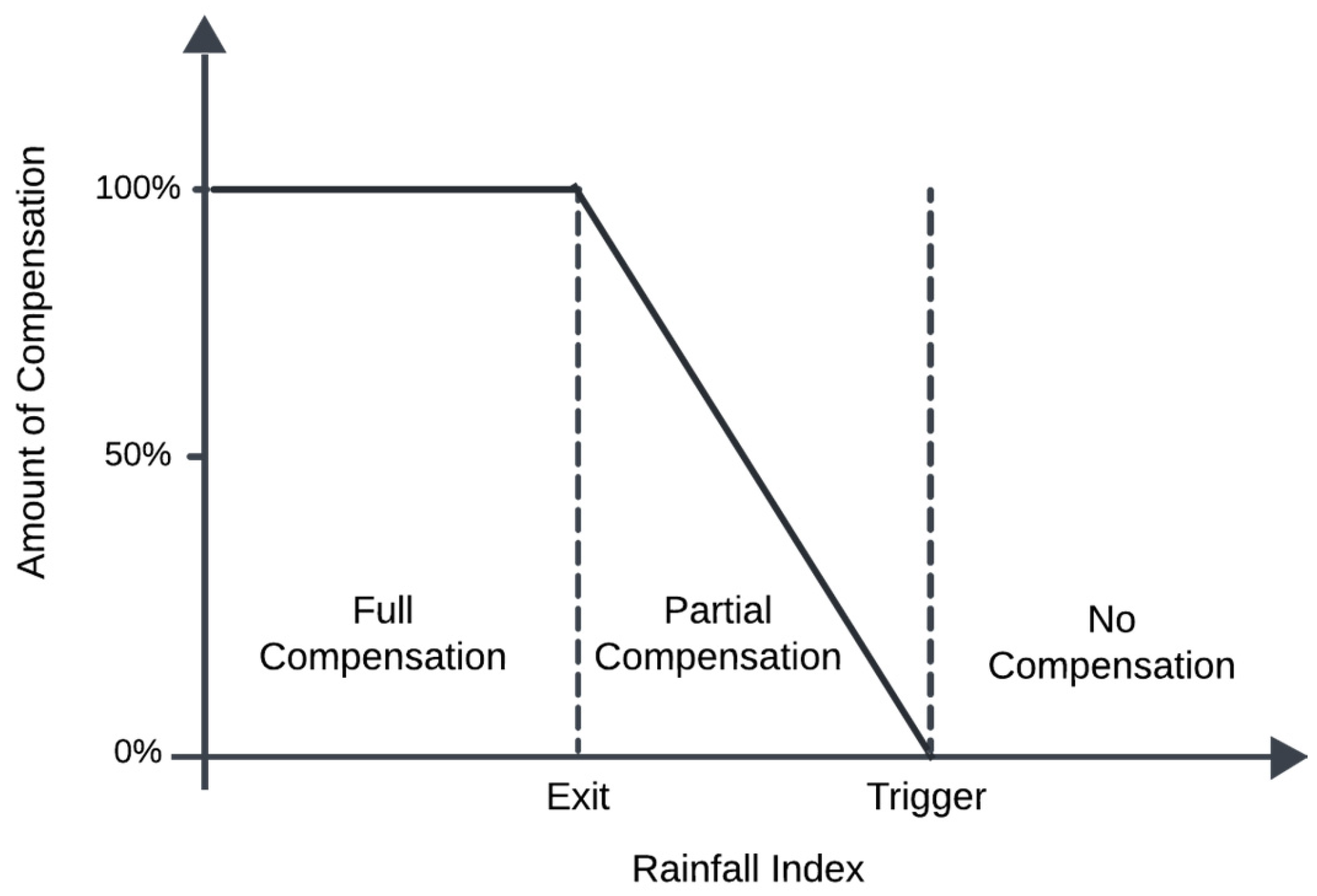
6.2.3. Agricultural Insurance Compensation Amount

The exit and trigger rainfall indices were adopted in determining the amount of compensation received by farmers in addition to being used in premium calculations. The maximum compensation was measured based on the costs required to cultivate corn in a growing season. The process required the submission of the claims for compensation after harvest, and the average total rainfall during the index window period was considered. Similar to premium calculations, the compensation scheme was divided into two categories based on the risk covered, including flood and drought. A detailed explanation of the compensation scheme for excess water risk leading to floods is presented in Figure 1. It is observed that the horizontal axis represents the rainfall index, and the vertical axis is the amount of compensation.

The information presented in Figure 1 shows that the exit index serves as the threshold for initiating insurance compensation while the trigger index is for full insurance compensation. The process of providing compensation starts when the rainfall index exceeds the exit index value and continues to increase up to the trigger index value. This mechanism is designed to protect farmers from the impact of floods that are capable of causing damage to crops [61]. Conversely, when the rainfall index remains below the exit index, no compensation is expected to be provided. The rainfall index that falls between the exit and trigger indices requires partial compensation from the insurer to the insured based on the following equation:

$$Y={\displaystyle \frac{\mathrm{R}\mathrm{a}\mathrm{i}\mathrm{n}\mathrm{f}\mathrm{a}\mathrm{l}\mathrm{l} \mathrm{I}\mathrm{n}\mathrm{d}\mathrm{e}\mathrm{x}-\mathrm{E}\mathrm{x}\mathrm{i}\mathrm{t}}{\mathrm{T}\mathrm{r}\mathrm{i}\mathrm{g}\mathrm{g}\mathrm{e}\mathrm{r}-\mathrm{E}\mathrm{x}\mathrm{i}\mathrm{t}}}\times M$$

(71)

where $Y$ represents the partial compensation given to the insured and $M$ is the insured amount value.

The compensation scheme when the insured risk is water shortage causing drought is presented in Figure 2. The horizontal axis represents the rainfall index while the vertical axis is the amount of compensation [21].

Figure 2 shows that the exit index represents the threshold for full insurance compensation while the trigger index serves as the threshold for initiating insurance compensation. The process of initiating the compensation is when the rainfall index falls below the trigger index and continues to increase up to the exit index. This mechanism is intended to protect farmers from the impact of a drought that is capable of causing crop losses. Conversely, when the rainfall index exceeds the trigger index, no compensation is expected to be provided. The situation when the rainfall index falls between the exit and trigger indices requires partial compensation for the insured based on the following equation:

$$Y={\displaystyle \frac{\mathrm{T}\mathrm{r}\mathrm{i}\mathrm{g}\mathrm{g}\mathrm{e}\mathrm{r}-\mathrm{R}\mathrm{a}\mathrm{i}\mathrm{n}\mathrm{f}\mathrm{a}\mathrm{l}\mathrm{l} \mathrm{I}\mathrm{n}\mathrm{d}\mathrm{e}\mathrm{x}}{\mathrm{T}\mathrm{r}\mathrm{i}\mathrm{g}\mathrm{g}\mathrm{e}\mathrm{r}-\mathrm{E}\mathrm{x}\mathrm{i}\mathrm{t}}}\times M$$

(72)

where $Y$ represents the partial compensation granted to the insured and $M$ denotes the insured value.

Partial compensation or indemnity denoted by $Y$ refers to the amount of coverage approved and provided by the insurance company to the participant who files a claim. In the context of rainfall index-based agricultural insurance, the maximum compensation is calculated as the total planting costs incurred by farmers from the start of the planting process to the harvest in a single season, denoted as $M$. The data from the Tasikmalaya Regency Agricultural Office showed that the total cost of planting corn per hectare per planting season was IDR 11,130,000. Therefore, the maximum compensation amount provided by the insurance company to the participant was $M=$ IDR 11,130,000.

7. Results

7.1. Corn Production and Rainfall Data

This study used secondary data that covered monthly corn production and daily rainfall in the Tasikmalaya Regency for the period from 2016 to 2023. The data were categorized based on seasonal periods to be in line with the corn planting patterns in the regency. The process led to three main periods, including Season I for January–April, Season II for May–August, and Season III for September–October. The calculations were conducted by aggregating the monthly corn production and daily rainfall data. The results of the calculations and the data plotted on corn production and rainfall in Tasikmalaya Regency from 2016 to 2023 are presented in

Table 2. Corn production and rainfall data.

Year	Corn Production (Ton)			Rainfall (mm)
	Season I	Season II	Season III	Season I	Season II	Season III
2016	38,224.33	37,620.49	31,733.05	1589.00	1181.00	1583.00
2017	27,032.93	10,402.79	51,949.46	1830.00	478.00	1619.40
2018	46,886.57	22,485.70	40,693.74	1069.30	282.20	1098.00
2019	22,592.43	21,365.82	13,346.48	1343.20	168.80	649.20
2020	25,273.73	48,144.17	20,969.97	1188.00	708.60	1237.90
2021	10,342.91	12,045.55	13,308.55	853.00	506.90	750.90
2022	5593.91	5286.51	13,515.13	879.40	550.20	957.00
2023	20,785.31	4205.02	5838.12	565.30	434.20	269.00

and Figure 3.

Figure 3 shows fluctuations in the data on corn production and rainfall annually. The fluctuations in corn production were influenced by several factors, including natural disasters, pest infestations, livestock disease outbreaks, and climate change, particularly changes in rainfall patterns. Meanwhile, rainfall data in Season II tended to be lower compared to I and III, which were influenced by seasonal patterns, specifically the transition between the dry and rainy seasons. These differences in rainfall patterns affected water availability for corn crops and subsequently the production levels. Therefore, rainfall had a strong relationship with corn production and agricultural production analysis, which contributed to the calculation of premiums in rainfall-based agricultural insurance.

7.2. Determination of Exit and Trigger Rainfall Indices Using Historical Burn Analysis

7.2.1. Determination of the Index Window

The index window or the insured period is determined using rainfall data that has the strongest correlation with corn production data for the same season period. The purpose of determining the index window is to identify the period that presents the greatest risk, leading to losses in the agricultural sector. The correlation coefficients were calculated using Equation (60), with the results presented in

Table 3. Correlation coefficients of rainfall against corn production.

	Corn Production	Season I	Season II	Season III
Rainfall
Season I		0.44	0.39	0.76
Season II		0.15	0.51	0.13
Season III		0.45	0.49	0.82

.

The rainfall and corn production data in Season III had the highest correlation value of 0.82, which was close to one. This shows a very strong relationship between rainfall and corn production in the season. Moreover, the positive value suggested a direct relationship and the trend showed that an increase in rainfall was followed by more corn production. Therefore, Season III, which was from September to December, was selected as the index window.

7.2.2. Determination of Cap Threshold Value

The Cap threshold value represents the maximum amount of rainfall calculated per dasarian. The determination of the Cap value is closely related to the daily potential evapotranspiration, which can be influenced by factors such as air temperature and humidity. The status of Indonesia as a tropical region shows the need to adjust the Cap value based on the characteristics of evapotranspiration in tropical areas.

Wati et al. [62] reported that the average potential evapotranspiration value in Java and Bali, Indonesia, was 5 mm per day. These data and the values presented in Table 1 led to the determination of the daily potential evapotranspiration value in the Tasikmalaya Regency as 5 mm per day. Therefore, the cap value for the ten-day period was calculated as 50 mm based on the following relationship:

$$\mathrm{C}\mathrm{a}\mathrm{p}=5 \mathrm{mm}/\mathrm{day}\times 10=50 \mathrm{mm}/\mathit{dasarian}.$$

7.2.3. Calculation of Dasarian Rainfall

The calculation of the dasarian rainfall $D_j, j=\mathrm{1,2},3$ was conducted only for daily rainfall data within the index window, which was Season III, from September to December for the 2016–2023 period. Each month was divided into three dasarian periods and the first covered the days one to ten. Moreover, the dasarian rainfall was calculated using Equation (61), as observed in the following example for September 2016, and the overall results are presented in

Table 4. Dasarian rainfall for each year.

Month	j	${\mathit{D}}_{\mathit{j}}$ (mm)
		2016	2017	2018	2019	2020	2021	2022	2023
September	1	99	1	81	1.8	37.7	8	49	0
	2	150	1	11	2.2	1	60	141	0.3
	3	120	181	77	2.4	152.8	115	92.9	0
October	1	180	251	5	2.8	186.8	13	105	1.5
	2	77	223	13	3.2	130.2	48.7	93.9	0
	3	151	28	67	0	101.5	72.1	60.3	22
November	1	65	174	294	114.6	185.6	123.1	104.5	33.7
	2	249	467	104	50.4	113.2	125.1	89.7	7.2
	3	193	42.4	199	26.8	99.8	57	126.5	62.5
December	1	116	39	140	162.2	114.3	46.1	22.4	113.6
	2	83	197	61	179.6	115	23.4	36	0
	3	0	15	46	148.2	0	59.4	35.8	28.2

.

$$D_1=\sum _{i=1}^{10}{h}_i=21+0+0+0+17+0+9+3+3+46=99 \mathrm{m}\mathrm{m}.$$

$$D_2=\sum _{i=11}^{20}{h}_i=33+0+8+1+0+23+3+11+63=150 \mathrm{m}\mathrm{m}.$$

$$D_3=\sum _{i=21}^{30}{h}_i=3+8+14+19+4+37+0+17+0+18=120 \mathrm{m}\mathrm{m}.$$

7.2.4. Determination of Dasarian Adjusted Rainfall

The dasarian adjusted rainfall was calculated based on two assumptions. The maximum value $D_{j:adj}, j=\mathrm{1,2},3$ was observed to be equal to the Cap value at 50 mm for each dasarian period. An example for September 2016 is presented as follows, while the overall results are in Table 5.

• ${\mathrm{D}}_1$= 99 mm was greater than the Cap value of 50 mm and the adjusted rainfall value $D_{j:adj}$ was set to 50 mm.
• ${\mathrm{D}}_2$ = 150 mm was greater than the Cap value of 50 mm and the adjusted rainfall value $D_{j:adj}$ was set to 50 mm.
• ${\mathrm{D}}_3$ = 120 mm was greater than the Cap value of 50 mm and the adjusted rainfall value $D_{j:adj}$ was set to 50 mm.

Table 5. Dasarian adjusted rainfall for each year.

Month	j	${\mathit{D}}_{\mathit{j}:\mathit{a}\mathit{d}\mathit{j}}$ (mm)
		2016	2017	2018	2019	2020	2021	2022	2023
September	1	50	1	50	1.8	37.7	8	49	0
	2	50	1	11	2.2	1	50	50	0.3
	3	50	50	50	2.4	50	50	50	0
October	1	50	50	5	2.8	50	13	50	1.5
	2	50	50	13	3.2	50	48.7	50	0
	3	50	28	50	0	50	50	50	22
November	1	50	50	50	50	50	50	50	33.7
	2	50	50	50	50	50	50	50	7.2
	3	50	42.4	50	26.8	50	50	50	50
December	1	50	39	50	50	50	46.1	22.4	50
	2	50	50	59	50	50	23.4	36	0
	3	0	15	46	50	0	50	35.8	28.2

Table 5. Dasarian adjusted rainfall for each year.

Month	j	${\mathit{D}}_{\mathit{j}:\mathit{a}\mathit{d}\mathit{j}}$ (mm)
		2016	2017	2018	2019	2020	2021	2022	2023
September	1	50	1	50	1.8	37.7	8	49	0
	2	50	1	11	2.2	1	50	50	0.3
	3	50	50	50	2.4	50	50	50	0
October	1	50	50	5	2.8	50	13	50	1.5
	2	50	50	13	3.2	50	48.7	50	0
	3	50	28	50	0	50	50	50	22
November	1	50	50	50	50	50	50	50	33.7
	2	50	50	50	50	50	50	50	7.2
	3	50	42.4	50	26.8	50	50	50	50
December	1	50	39	50	50	50	46.1	22.4	50
	2	50	50	59	50	50	23.4	36	0
	3	0	15	46	50	0	50	35.8	28.2

7.2.5. Calculation of Average Total Dasarian Adjusted Rainfall

The adjusted rainfall values were summed and averaged annually using Equation (62). An example of the calculation for the average total rainfall in 2016 is presented as follows and the overall results are in

Table 6. Average total dasarian adjusted rainfall $\left({\overline{A}}_{m:adj}\right)$ and its ascending $\left({\overline{A}}_{m:adj}\uparrow \right)$ for each year.

Year	$\mathit{m}$	${\overline{\mathit{A}}}_{\mathit{m}:\mathit{a}\mathit{d}\mathit{j}}$ (mm)	$\mathbf{Year}\uparrow$	$\mathit{m}\uparrow$	${\overline{\mathit{A}}}_{\mathit{m}:\mathit{a}\mathit{d}\mathit{j}}\uparrow$ (mm)
2016	1	45.8333	2023	8	16.0750
2017	2	35.5333	2019	4	24.1000
2018	3	39.5833	2017	2	35.5333
2019	4	24.1000	2018	3	39.5833
2020	5	40.7250	2020	5	40.7250
2021	6	40.7667	2021	6	40.7667
2022	7	45.2667	2022	7	45.2667
2023	8	16.0750	2016	1	45.8333

.

$${\overline{A}}_{m:adj}={\displaystyle \frac{50+50+50+50+50+50+50+50+50+50+50+0}{12}}={\displaystyle \frac{550}{12}}=45.8333 \mathrm{mm}$$

7.2.6. Arrangement of Average Total Dasarian Adjusted Rainfall

The average total dasarian adjusted rainfall ${\overline{A}}_{m:adj}$ was later arranged in ascending order from the smallest to the largest value in Table 6. This arrangement was used to determine the exit and trigger rainfall indices.

7.2.7. Determination of the Exit and Trigger Rainfall Indices

The exit index value was determined based on the lowest adjusted average total rainfall data after the ascending arrangement and using Equation (63). The results presented in Table 6 showed that the exit value was set at 16.0750 mm. Meanwhile, the trigger index value $G$ was determined based on the percentile of the average total dasarian adjusted rainfall data for each year. It was calculated using Equation (64) and the smallest data point represented the 1st percentile, while the largest data point was the 100th percentile, with the values recorded presented in

Table 7. Trigger index values (mm).

Percentile	Trigger ($\mathit{G}$)	Percentile	Trigger ($\mathit{G}$)
1%	16.6368
5%	18.8838	55%	40.5537
10%	21.6925	60%	40.7333
15%	24.6717	65%	40.7479
20%	28.6733	70%	40.7625
25%	32.6750	75%	41.8917
30%	35.9383	80%	43.4667
35%	37.3558	85%	45.0417
40%	38.7733	90%	45.4367
45%	39.7546	95%	45.6350
50%	40.1542	100%	45.8333

.

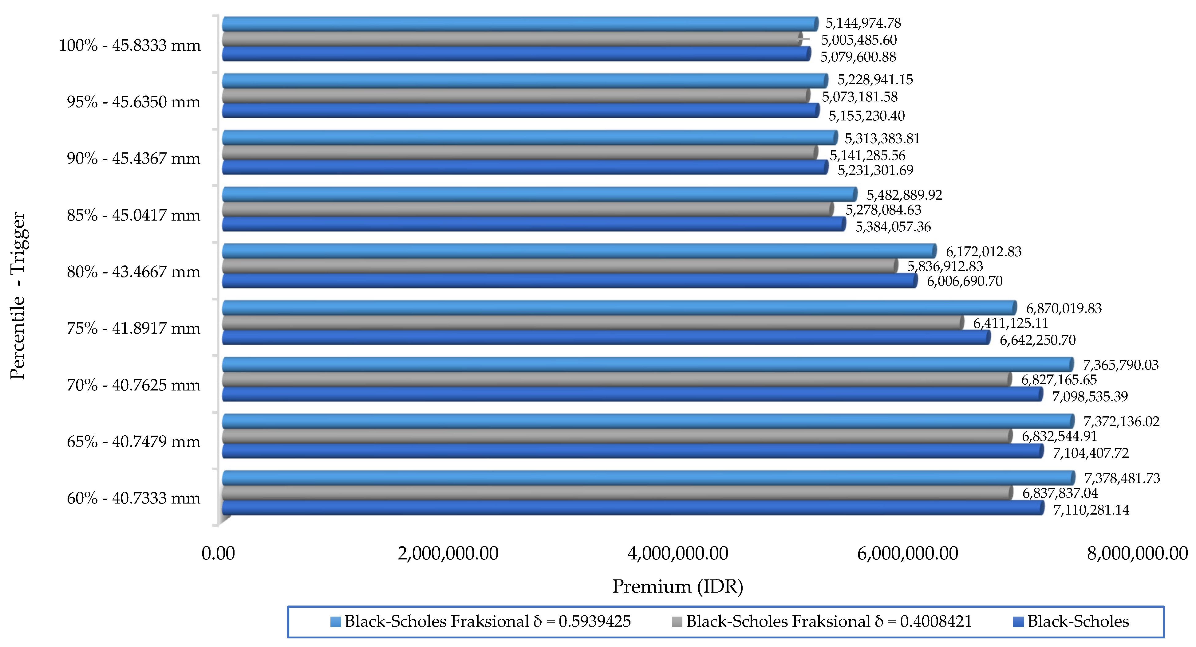
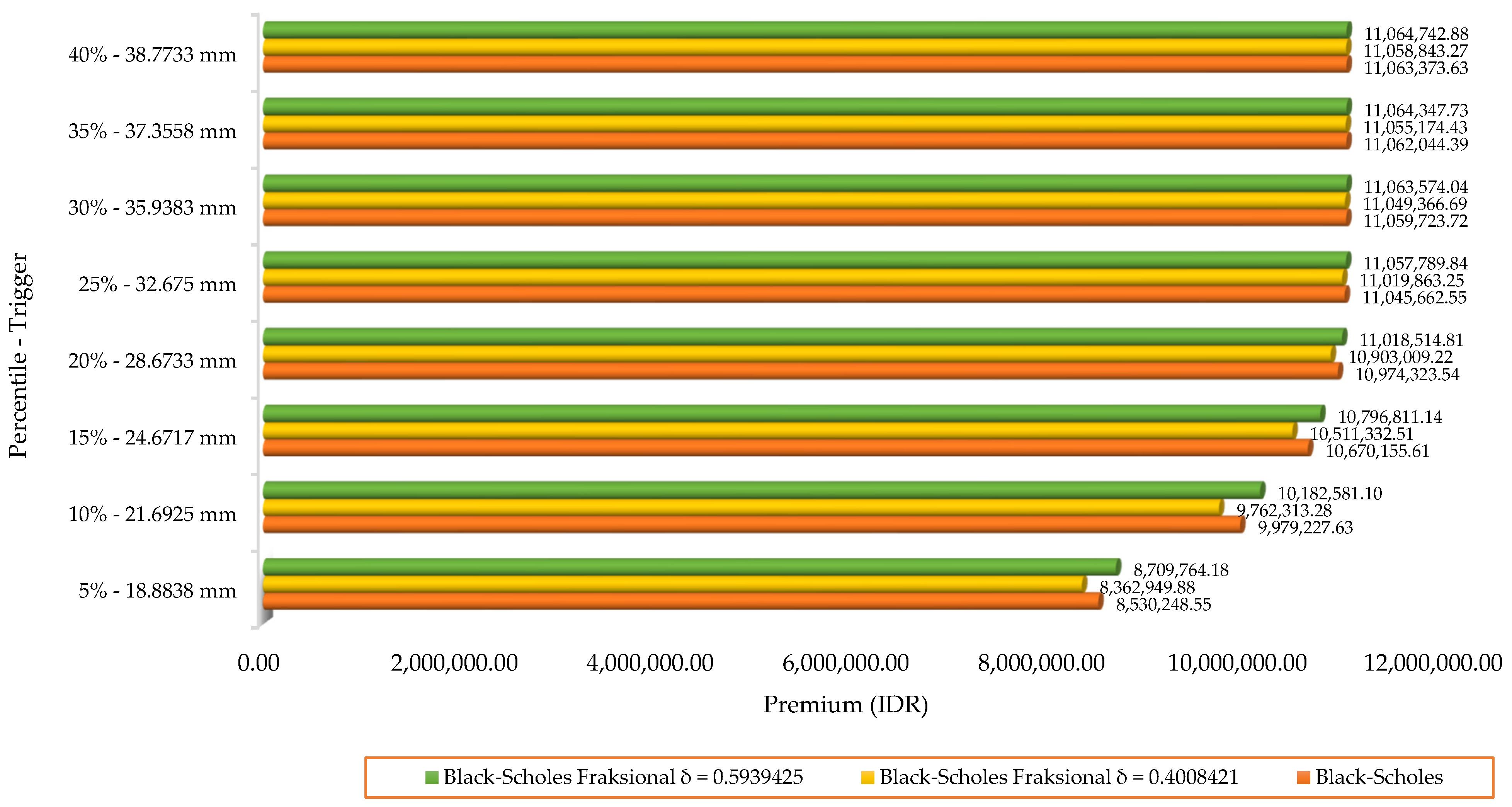
7.3. Calculation of Premiums Using the Standard and Fractional Black–Scholes Models

7.3.1. Calculation of Premiums Using the Standard Black–Scholes Model

The standard Black–Scholes model can be used in calculating agricultural insurance premiums when the normality test assumption is satisfied. This test was conducted to determine that the natural logarithm of Season III data was in line with the normal distribution. This was achieved using the Anderson–Darling test at a 5% significance level through the application of Minitab 18 software. The calculation showed that the p-value was 0.315 and the value confirmed that the natural logarithm of the Season III data, covering the months from September to December, followed a normal distribution. Therefore, the Black–Scholes model could be applied to calculate the agricultural insurance premium.

The process of calculating the premiums was divided into two focuses based on the covered risks, including flood and drought. The aspect of flood risk was determined using Equation (67), while the drought risk was based on Equation (69). Furthermore, the calculation of cumulative distribution values was performed through Equation (65). The data used were from the insurance period $T$ of 0.3333, derived from a planting cycle of four months and a risk-free interest rate of $r=\mathrm{l}\mathrm{n}(i+1)=1.753164\%$, based on the assumption of $i$ as the Bank Indonesia rate. The other factor was the standard deviation of rainfall $\sigma$, which was determined using the average total annual rainfall, as presented in Table 7.

$$\overline{u}={\displaystyle \frac{1}{n-1}}\sum _{m=2}^n\mathrm{l}\mathrm{n}\left({\displaystyle \frac{{\overline{A}}_m}{{\overline{A}}_{m-1}}}\right)=-0.149678041,$$

$$\sigma =\sqrt{{\displaystyle \frac{1}{n-2}}\left({\sum }_{k=2}^n{\left(u_k-\overline{u}\right)}^2\right)}=\sqrt{{\displaystyle \frac{1}{n-2}}\left({\sum }_{m=2}^n{\left(\mathrm{l}\mathrm{n}\left({\displaystyle \frac{{\overline{A}}_{m;adj}}{{\overline{A}}_{m-1;adj}}}\right)-\overline{u}\right)}^2\right)}=0.4364468.$$

The premium for the flood risk was calculated using the Black–Scholes model based on the highest total rainfall value of ${\overline{A}}_0$, which was recorded as 45.8333 in Table 6, and the trigger value $G$ in Table 7. The percentile value for the flood risk was based on the rainfall intensity in

Table 8. Rainfall characteristics for flood risk.

No	Rainfall (mm/day)	Criteria
1	0.5–20	Light Rain
2	20–50	Moderate Rain
3	50–100	Heavy Rain
4	100–150	Very Heavy Rain
5	$>$150	Extreme Rain

[63].

Categories 3 to 5 represent heavy to extreme rain and have the potential to cause significant damage due to flood risk. This is because the rainfall with the intensity tends to cause excessive water accumulation, which is capable of disrupting agricultural activities, damaging crops, and reducing yields. Therefore, the percentile value for flood risk was ${\displaystyle \frac{3}{5}}\times 100=60\%$. The trend showed that the percentile values started from the 60th percentile and progressed through the 65th, 70th, 75th, 80th, 85th, 90th, 95th, and 100th percentiles.

The cumulative distribution value $d_2$ was calculated using Equation (65). An example for the 60th percentile with a trigger index value of 40.7333 is presented as follows.

$$d_2={\displaystyle \frac{\ln \left(\frac{45.8333}{40.7333}\right)+\left(1.753164-\frac{{(0.4364468)}^2}{2}\right)(0.3333)}{(0.4364468)\sqrt{0.3333}}}=0.365372.$$

The premium for flood risk was calculated using Equation (67). An example for the 60th percentile with a coverage value $M=$ IDR 11,130,000, insurance period $T=0.3333$, and cumulative distribution probability $N(0.365372)=0.642583$ is stated as follows, while the results for all percentiles are in

Table 9. Agricultural insurance premiums using the Black–Scholes model for flood risk.

Percentile	Trigger (mm)	$\mathit{N}({\mathit{d}}_2)$	Premium (IDR)
60%	40.7333	0.642583	7,110,281.14
65%	40.7479	0.642025	7,104,407.72
70%	40.7625	0.641522	7,098,535.39
75%	41.8917	0.600285	6,642,250.70
80%	43.4667	0.542847	6,006,690.70
85%	45.0417	0.486578	5,384,057.36
90%	45.4367	0.472773	5,231,301.69
95%	45.6350	0.465898	5,155,230.40
100%	45.8333	0.459063	5,079,600.88

.

$$\mathrm{P}\mathrm{r}\mathrm{e}\mathrm{m}\mathrm{i}\mathrm{u}\mathrm{m}=\mathrm{I}\mathrm{D}\mathrm{R} \mathrm{11,130,000}{e}^{-(1.753164)(0.3333)}N(0.365372)=\mathrm{I}\mathrm{D}\mathrm{R} \mathrm{7,110,281.14}.$$

The premium was observed to vary according to the level of rainfall intensity measured and the risk faced. It was applicable to one planting season and required to be paid at the start. Furthermore, the premium structure reflected the principle of fairness because a reduction was observed in the value as the number of participants in insurance program increased. Another important observation was that the amount depended on the trigger index value $G$. This was identified from the fact that a smaller $G$ value led to a higher ${N(d}_2)$ and subsequently an increase in the premium amount.

The calculation of the premium for drought risk using the Black–Scholes model was based on the smallest value of ${\overline{A}}_0$ for drought, which was 16.0750 in Table 6, and the trigger $G$ derived from the percentile calculation of the Season III rainfall data in Table 7. The percentile value for drought risk was also based on the associated rainfall intensity in

Table 10. Rainfall characteristics for drought risk.

No	Rainfall (mm/day)	Criteria
1	$\le$1.000	Very Dry
2	1.001–2.000	Dry
3	2.001–3.000	Moderate
4	3.001–4.000	Wet
5	$>$4.000	Very Wet

.

Categories 2 and 1 reflect dry to very dry rainfall conditions, which represent the very low rainfall levels and increase the potential impact on water availability. Rainfall intensities within this range show a significant increase in drought risk, which negatively affects crop yields. Therefore, the percentile value used for drought risk is ${\displaystyle \frac{2}{5}}\times 100=40\%$. The percentile values for drought risk start from the 5th percentile, progressing through the 10th, 15th, 20th, 25th, 30th, 35th, and 40th percentiles.

The cumulative distribution value $d_2$ was calculated using Equation (65). An example for the 5th percentile with a trigger index value of 18.8838 is presented as follows.

$$d_2={\displaystyle \frac{\ln \left(\frac{16.0750}{18.8838}\right)+\left(1.753164-\frac{{(0.4364468)}^2}{2}\right)(0.3333)}{(0.4364468)\sqrt{0.3333}}}=-0.741904.$$

The premium for drought risk was calculated using Equation (69). An example for the 5th percentile with a coverage value $M=$ IDR 11,130,000, insurance period $T=0.333$, and cumulative distribution probability $N(0.741904)=0.770927$ is presented as follows, and the results for all the percentiles are in

Table 11. Agricultural insurance premiums using the Black–Scholes model for drought risk.

Percentile	Trigger (mm)	$\mathit{N}({-\mathit{d}}_2)$	Premium (IDR)
5%	18.8838	0.770927	8,530,248.55
10%	21.6925	0.901851	9,979,227.63
15%	24.6717	0.964296	10,670,155.61
20%	28.6733	0.991789	10,974,323.54
25%	32.6750	0.998238	11,045,662.55
30%	35.9383	0.999509	11,059,723.72
35%	37.3558	0.999719	11,062,044.39
40%	38.7733	0.999839	11,063,373.63

.

$$\mathrm{P}\mathrm{r}\mathrm{e}\mathrm{m}\mathrm{i}\mathrm{u}\mathrm{m}=\mathrm{I}\mathrm{D}\mathrm{R} \mathrm{11,130,000}{e}^{-(1.753164)(0.3333)}N(0.741904)=\mathrm{I}\mathrm{D}\mathrm{R} \mathrm{8,530,428.55}.$$

The premium varied as a reflection of the adjustment to the intensity of the rainfall and ensured suitable protection against the potential losses due to drought risk. It was applicable to one planting season and required to be paid at the start of the season. The aim was to ensure farmers felt secure in conducting agricultural activities without worrying about drought risk during the planting period. The premium amount depended on the $G$ value. It was observed that a larger $G$ value led to an increase in $N(-d_2)$ and subsequently caused a higher premium.

7.3.2. Calculation of Premiums Using the Fractional Black–Scholes Model

The calculation of the premium using the fractional Black–Scholes model was initiated by identifying the long-term impact and determining the additional fractional order parameter. The identification of the long-term impact was achieved by calculating the Hurst exponent from rainfall data using the rescaled range statistics $(R/S)$ method. The Hurst exponent was estimated with the assistance of R Studio 4.3.2 software, which produced a value of $H=0.8917389$. The value is within the interval $0.5<\mathrm{H}<1$ and this shows that the rainfall data exhibits a long-term dependence. Meanwhile, the fractional order parameter was determined through the adoption of the Geweke and Porter-Hudak method. The estimation was also conducted using R Studio and the fractional order parameter $\delta$ value produced was $0.4008421$.

The significance of the fractional order parameter was required to be tested in order to assess the effect on model. The hypothesis used was $H_0$: $\widehat{\delta }=0$ against $H_1$: $\widehat{\delta }\ne 0$ and the test was conducted at a 5% significance level using R Studio software. Based on the calculations, the estimator $\widehat{\delta }=0.4008421$ with a standard error $E(\widehat{\delta })=0.09852247$ produced a $Z_{\mathrm{c}\mathrm{a}\mathrm{l}\mathrm{c}\mathrm{u}\mathrm{l}\mathrm{a}\mathrm{t}\mathrm{e}\mathrm{d}}$ of 4.068533. Moreover, the critical value of the standard normal distribution at a significance level of $\alpha =5\%$ was $Z_{1-{\displaystyle \frac{0.05}{2}}}=1.959964$. The trend showed that $Z_{\mathrm{c}\mathrm{a}\mathrm{l}\mathrm{c}\mathrm{u}\mathrm{l}\mathrm{a}\mathrm{t}\mathrm{e}\mathrm{d}}>Z_{1-{\displaystyle \frac{0.05}{2}}}$ and this was an indication the fractional order parameter was significant for the model. The estimated confidence interval for the fractional order parameter at a 95% confidence level was calculated using the formula $\widehat{\delta }+Z_{{\displaystyle \frac{\alpha }{2}}}·SE\left(\widehat{\delta }\right)<\delta <\widehat{\delta }+Z_{1-{\displaystyle \frac{\alpha }{2}}}·SE(\widehat{\delta })$ and produced $0.2077416<\delta <0.5939426$. The $\delta$ is within the interval $-0.5<\delta <0.5$, which is confirmed to be reliable.

The calculation of the premium for flood risk using the fractional Black–Scholes model was conducted based on ${\overline{A}}_0$ for flood, which was the largest value of 45.8333 from Table 6, and the $G$ derived from the percentiles of the quarterly rainfall data in Table 7. The percentile ranged from 60%, 65%, 70%, 75%, 80%, 85%, 90%, 95%, to 100% based on the rainfall intensity related to flood risk, as presented in Table 9.

The cumulative distribution value $d_2$ was calculated using Equation (70). An example for the 60th percentile with a trigger index value of 40.7333 is presented as follows:

$$d_2={\displaystyle \frac{\ln \left(\frac{45.8333}{40.7333}\right)+\left(1.753164\right)(0.3333)-\frac{1}{2}{\left(0.4364468\right)}^2{(0.3333)}^{2(0.4008421)}}{(0.4364468)\sqrt{{(0.3333)}^{2(0.4008421)}}}}=0.300152.$$

The premium for flood risk was calculated using Equation (67). An example for agricultural insurance premium based on the rainfall index for flood risk at the 60th percentile, with a coverage value $M=$ IDR 11,130,000, insurance period $T=0.333$, and cumulative distribution probability $N(0.300152)=0.617969$, is presented as follows:

$$\mathrm{P}\mathrm{r}\mathrm{e}\mathrm{m}\mathrm{i}\mathrm{u}\mathrm{m}=\mathrm{I}\mathrm{D}\mathrm{R} \mathrm{11,130,000}{e}^{-(1.753164)(0.3333)}N(0.300152)=\mathrm{I}\mathrm{D}\mathrm{R} \mathrm{6,837,927.34}.$$

The results obtained for all percentiles are presented in

Table 12. Agricultural insurance premiums using the fractional Black–Scholes model for flood risk with fractional order parameter $\delta =0.4008421$ and $\delta =0.5939425$.

Percentile	Trigger (mm)	$\mathit{\delta }=0.4008421$		$\mathit{\delta }=0.5939425$
		$\mathit{N}({\mathit{d}}_2)$	Premium (IDR)	$\mathit{N}({\mathit{d}}_2)$	Premium (IDR)
60%	40.7333	0.617969	6,837,837.04	0.666808	7,378,481.73
65%	40.7479	0.617476	6,832,544.91	0.666236	7,372,136.02
70%	40.7625	0.616990	6,827,165.65	0.665663	7,365,790.03
75%	41.8917	0.579392	6,411,125.11	0.620860	6,870,019.83
80%	43.4667	0.527500	5,836,912.83	0.557782	6,172,012.83
85%	45.0417	0.476999	5,278,084.63	0.495507	5,482,889.92
90%	45.4367	0.464636	5,141,285.56	0.480188	5,313,383.81
95%	45.6350	0.458481	5,073,181.58	0.472556	5,228,941.15
100%	45.8333	0.452363	5,005,485.60	0.464969	5,144,974.78

. Moreover, the premium was also calculated through the fractional order parameter $\delta$ obtained from the estimated interval. It was observed from the interval estimation that the upper bound of the fractional order parameter $\delta$ was 0.5939425. The results of the premium calculated for all percentiles are presented in Table 12.

The information in Table 12 shows a difference between the premiums calculated using the standard and fractional Black–Scholes models. The difference is associated with the consideration of the fractional order parameter $\delta$ in the fractional Black–Scholes model, which leads to the dependence of the premium payments on a specific time parameter. The model also offers a variety of premium options but with the consequence of higher costs. This shows the potential of the fractional Black–Scholes model as an innovative solution for risk management in agricultural sector, specifically in response to changing rainfall patterns.

The calculation of premium for drought risk using the fractional Black–Scholes model was based on ${\overline{A}}_0$, which was 16.0750 as the smallest value in Table 6, and the $G$ in Table 7. The percentile values were 5%, 10%, 15%, 20%, 25%, 30%, 35%, and 40% based on the rainfall intensity associated with drought risk in Table 11.

The cumulative distribution value $d_2$ was calculated using Equation (70). An example for the 5th percentile with a trigger index value of 18.8838 is presented as follows:

$$d_2={\displaystyle \frac{\ln \left(\frac{16.0750}{18.8838}\right)+\left(1.753164\right)(0.3333)-\frac{1}{2}{\left(0.4364468\right)}^2{(0.3333)}^{2(0.4008421)}}{(0.4364468)\sqrt{{(0.3333)}^{2(0.4008421)}}}}=-0.692829.$$

The premium for drought risk was calculated using Equation (69). Therefore, the agricultural insurance premium based on the rainfall index for drought risk at the 5th percentile, with a coverage value $M=$ IDR 11,130,000, insurance period $=0.333$, and cumulative distribution probability $N(0.692829)=0.755792$, is presented as follows:

$$\mathrm{P}\mathrm{r}\mathrm{e}\mathrm{m}\mathrm{i}\mathrm{u}\mathrm{m}=\mathrm{I}\mathrm{D}\mathrm{R} \mathrm{11,130,000}{e}^{-(1.753164)(0.3333)}N(0.692829)=\mathrm{I}\mathrm{D}\mathrm{R} \mathrm{8,362,949.88}.$$

The results for all percentiles are shown in

Table 13. Agricultural insurance premiums using the Fractional Black–Scholes model for drought risk with fractional order parameter $\delta =0.4008421$ and $\delta =0.5939425$.

Percentile	Trigger (millimeter)	$\mathit{\delta }=0.4008421$		$\mathit{\delta }=0.5939425$
		$\mathit{N}(-{\mathit{d}}_2)$	Premium (IDR)	$\mathit{N}(-{\mathit{d}}_2)$	Premium (IDR)
5%	18.8838	0.755792	8,362,949.88	0.787124	8,709,764.18
10%	21.6925	0.882250	9,762,313.28	0.920228	10,182,581.10
15%	24.6717	0.949943	10,511,332.51	0.975743	10,796,811.14
20%	28.6733	0.985344	10,903,009.22	0.995783	11,018,514.81
25%	32.6750	0.995906	11,019,863.25	0.999334	11,057,789.84
30%	35.9383	0.998572	11,049,366.69	0.999863	11,063,574.04
35%	37.3558	0.999098	11,055,174.43	0.999927	11,064,347.73
40%	38.7733	0.999430	11,058,843.27	0.999963	11,064,742.88

. Moreover, the premium calculation was conducted through the fractional order parameter $\delta$ obtained from the estimated interval. It was observed from the interval estimation calculation that the upper bound of the fractional order parameter $\delta$ was 0.5939425. The results of the premium calculated for all percentiles are shown in Table 13.

The information in Table 13 showed a difference between the premiums calculated using the standard and fractional Black–Scholes models. The difference was associated with the consideration of the fractional order parameter $\delta$ in the fractional Black–Scholes model, which led to the dependence of the premium payments on a specific time parameter. This adds a higher degree of flexibility in implementing agricultural insurance programs. Therefore, the fractional Black–Scholes model can be an innovative method for managing risks in the agricultural sector, particularly in facing the dynamics of changing rainfall patterns.

7.4. Determination of Agricultural Insurance Compensation Using Historical Burn Analysis

The mechanism for providing compensation in rain index-based agricultural insurance consists of three categories, including full, partial, and no compensation. Similar to the premium determination, compensation is divided into two main focuses based on the risks covered, which are flood and drought. The flood risk is associated with high rainfall intensity that exceeds the threshold set, while the drought risk is due to low rainfall below the required threshold. The data used in determining compensation were the exit and trigger rainfall indices according to percentiles. This showed that the 60th, 65th, 70th, 75th, 80th, 85th, 90th, 95th, and 100th percentiles were used for the flood risks based on the calculations in Section 7.3.1. Meanwhile, the 5th, 10th, 15th, 20th, 25th, 30th, 35th, and 40th percentiles were used to determine the compensation for drought risks.

The concept of providing compensation in rain index-based agricultural insurance for flood risks is presented in Figure 1. It is observed that compensation is provided when the rainfall index exceeds the exit index value of 16.0750 and continues to increase up to the trigger index value based on the percentile. However, when the rainfall index is below the exit index value of 16.0750, no compensation is provided. Another condition is that partial compensation is provided according to Equation (71), when the rainfall index is between the exit and trigger values. An example of partial compensation calculated at the 60th percentile with a trigger value of 40.7333 and a coverage amount ($M$) of IDR 11,130,000 for the rainfall index of 17.075 is presented as follows, while the results for different rainfall indices are in

Table 14. Agricultural insurance compensation for flood risk at the 60th percentile.

Percentile	Exit	Trigger	Rainfall Index (mm)	Compensation (IDR)
60%	16.0750	40.7333	$\le$16.0750	0
			17.075	451,368.71
			18.075	902,737.41
			19.075	1,354,106.12
			21.075	2,256,843.53
			23.075	3,159,580.94
			26.075	4,513,687.06
			28.075	5,416,424.47
			30.075	6,319,161.88
			32.075	7,221,899.29
			34.075	8,124,636.70
			36.075	9,027,374.11
			38.075	9,930,111.52
			39.075	10,381,480.23
			40.075	10,832,848.94
			$\ge$40.7333	11,130,000

.

$$Y={\displaystyle \frac{17.075-16.0750}{40.7333-16.0750}}\times \mathrm{I}\mathrm{D}\mathrm{R} \mathrm{11,130,000}=\mathrm{I}\mathrm{D}\mathrm{R} \mathrm{451,368.71}.$$

The compensation amount in rain index-based agricultural insurance was determined by comparing the rainfall level to the threshold values of the exit and trigger rainfall indices. The results showed that when the rainfall exceeded the trigger value of 40.7333 mm at the 60th percentile, the farmer was entitled to receive full compensation due to the high flood risk. However, no compensation was provided when the rainfall was lower than the exit value of 16.0750 mm at the 60th percentile, because the risk criteria and conditions were not satisfied. It was further observed that partial compensation was paid when the rainfall was between the exit value of 16.0750 mm and the trigger value of 40.7333 mm. The amount was determined through a proportional calculation associated with the rainfall level during the planting season that posed a high flood risk.

The concept of providing compensation for the covered risk of drought is presented in Figure 2. The compensation was designed to be initiated when the rainfall index was below the trigger index value according to the percentile and continued to increase up to the exit index value of 16.0750. Meanwhile, no compensation was provided when the rainfall index exceeded the trigger index value. Another condition is that partial compensation is provided based on Equation (72), when the rainfall index is between the exit and trigger values. An example of the partial compensation calculated at the 5th percentile with a trigger value of 18.8838 and a coverage amount ($M$) of Rp 11,130,000 for the rainfall index of 18.575 is presented as follows, while the results for rainfall indices are in

Table 15. Agricultural insurance compensation for drought risk at the 5th percentile.

Percentile	Exit	Trigger	Rainfall Index (mm)	Compensation (IDR)
5%	16.0750	18.8838	$\le$16.0750	11,130,000
			16.575	9,148,691.59
			17.075	7,167,383.18
			17.575	5,186,074.77
			18.075	3,204,766.36
			18.575	1,223,457.94
			$\ge$18.8838	0

.

$$Y={\displaystyle \frac{18.8838-18.575}{18.8838-16.0750}}\times \mathrm{I}\mathrm{D}\mathrm{R} \mathrm{11,130,000}=\mathrm{I}\mathrm{D}\mathrm{R} \mathrm{1,223,457.94}.$$

The compensation amount in rain index-based agricultural insurance was determined by comparing the rainfall level to the exit and trigger index values. This was observed from the provision of full compensation for farmers due to the high risk of drought damage when the rainfall was lower than the exit value of 16.0750 mm at the 5th percentile. However, no compensation was provided when the rainfall exceeded the trigger value of 18.8838 mm at the 5th percentile, because the risk criteria and conditions were not satisfied. It was further observed that partial compensation was paid when the rainfall was between 16.0750 and 18.8838 mm according to a proportional calculation based on the rainfall level during the planting season with the high risk of drought.

The same exit index rainfall value, which was the lowest total average rainfall, was used to calculate the compensation for both flood and drought risks. However, there was a difference in the definition of the rainfall trigger index value for each covered risk. The setting of the trigger index at the 60th percentile for flood risks showed that the insurance participant was expected to receive compensation when the rainfall was greater than or equal to the trigger index value at the percentile. Meanwhile, the preference for the 5th percentile in drought risks showed that the insurance participant was expected to receive compensation when the rainfall was less than or equal to the trigger index value at this percentile. A higher percentile caused an increase in rainfall trigger index value and subsequently led to a wider compensation eligibility range. Therefore, the possibility of insurance participants receiving compensation increased with a higher percentile.

European-style options can only be executed on the last day of the term or the expiration date. Claims can be filed based on a similar mechanism in rainfall index-based agricultural insurance, either using the rainfall recorded on the last day of the insurance contract or calculated as the average rainfall over the contract period. Compensation in the flood risk protection scheme is provided when the recorded rainfall exceeds the trigger rainfall index value set according to the percentile. Meanwhile, compensation for drought risk is provided when the recorded rainfall is lower than the trigger rainfall index value set according to the percentile.

8. Discussion

The Black–Scholes model can be applied to agricultural insurance premiums due to the similarities shared in relation to the mechanism of calculating financial option prices. In the financial context, options are defined as contracts that provide the holder with the right but not the obligation to buy or sell an asset at a predetermined price and time. Meanwhile, agricultural insurance with a specific focus on index-based rainfall is defined as a contract that grants the policyholder the right to receive compensation in the event of an extreme weather condition, such as a drought or flood, in line with the criteria set by the index.

The use of the Black–Scholes model is expected to provide more optimal insurance premium values due to its focus on historical data and the objective consideration of market conditions. Moreover, the premium determined is designed to be applicable for the entire planting season and paid at the start. This mechanism allows farmers to gain the certainty of protection against risks capable of threatening their harvest throughout the season. However, in practice, not all farmers realize the importance of insurance from the start of the planting season. Several new farmers only feel the need for insurance once the season is underway and signs of extreme weather start to appear. This leads to a challenge in implementing the agricultural insurance scheme based on upfront premium payments using the Black–Scholes model.

The fractional Black–Scholes model offers a more flexible method for the premium payment mechanism in rainfall index-based agricultural insurance by considering the fractional order. This model allows for premium payments at the start of the planting season and other periods according to the value of the fractional order parameter. The premiums paid can become more expensive than the standard Black–Scholes model but provide farmers with greater flexibility in participating in the insurance program. Therefore, this model is more adaptive in accommodating the needs of farmers who only realize the importance of insurance once the planting season has already started.

The application of the fractional Black–Scholes model in agricultural insurance premium calculations was supported by the identification of the risks covered in the form of floods and droughts. The rainfall trigger index value was applied in the flood risk protection scheme based on specific percentiles that reflected the relevant risk levels for each extreme weather category. This method aimed to ensure that the insurance protection scheme was in line with the severity of the risks faced by farmers. The premium calculations for rain index-based agricultural insurance using the standard and fractional Black–Scholes models for each of the flood and drought risks in the Tasikmalaya Regency are presented in Figure 4 and Figure 5.

The rainfall trigger index values used for the calculation of premiums for both models represented the characteristics of rainfall with the potential to cause losses, either from floods or droughts. For example, the premium to be paid using the Black–Scholes model for flood risk at the 60th percentile with the rainfall trigger index value of 40.7333 mm was IDR 7,110,281.14. Meanwhile, the premium expected using the fractional Black–Scholes model was IDR 6,837,837.04 for the fractional period of 0.4008421 and IDR 7,378,481.73 for 0.5939425. Similar calculations were applied to drought risk at the 5th percentile with the rainfall trigger index value of 18.8838, which were IDR 8,530,248.55 and IDR 8,362,949.88 for the fractional period of 0.4008421, and IDR 8,709,764.18 for 0.5939425.

The calculations using the fractional Black–Scholes model with the fractional order of $\delta =0.4008421$ produced a lower premium than the standard model. This could increase the risk for the insurance company but was considered implementable for a large number of participants in order to adequately diversify the risk. Meanwhile, the fractional order of $\delta =0.5939425$ produced a higher premium than the standard model. This could lead to a fairer risk for both the farmers and insurance company and was considered applicable to relatively small or large participants.

9. Conclusions

In conclusion, agricultural crop farming was observed to be highly vulnerable to changes in rainfall patterns. Crop growth was confirmed to be heavily dependent on water availability, including scarcity, nonexistence, or even excess. This increased the risk of losses due to extreme rainfall changes, which could disrupt crop production. Therefore, rainfall index-based climate insurance was proposed as an adaptation strategy for farmers to maintain the stability of corn production. In this scheme, farmers were expected to receive compensation not tied to harvest yields but based on time and the rainfall index parameter. The purpose was to reduce the administrative costs of claims based on the harvested land area.

The process led to the adoption of the standard and fractional Black–Scholes models for calculating agricultural insurance premiums based on rainfall indices, with a focus on two main risks, including floods and droughts. The standard Black–Scholes model established the premium payments for the entire planting season and were required to be paid at the start. However, farmers often realized the need for protection and wished to enroll in insurance when the season was already underway. This led to the development of the fractional Black–Scholes model, with due consideration for fractional order parameters in order to provide flexibility in the premium payment mechanism. The method allowed for premium payments to be made at the start of the season, and periods were adjusted according to the fractional order applied. This flexibility led to higher premiums and ensured the principle of fairness for both the insurance company and farmers.

This study is expected to serve as a guide for insurance companies in evaluating the impact of climate risks in order to financially assess the viability of the program. Moreover, it could protect farmers from economic losses caused by climate disasters, specifically rainfall. The results are also expected to assist the Tasikmalaya Regency Government’s Agriculture Department in formulating policies and programs for socializing with farmers participating in insurance programs. Some challenges identified include other factors such as temperature and humidity, which had the capacity to influence index-based agricultural insurance. Therefore, other climate parameters should be added to ensure more adaptive premiums in line with varying climatic conditions and to effectively mitigate risks.

References

1. Kraus, K.; Kraus, N.; Pochenchuk, G. Principles, Assessment and Methods of Risk Management of Investment Activities of the Enterprise. VUZF Rev. 2021, 6, 45–58. [Google Scholar] [CrossRef]
2. Giudice, M.D.; Evangelista, F.; Palmaccio, M. Defining the Black and Scholes Approach: A First Systematic Literature Review. J. Innov. Entrep. 2015, 5, 5. [Google Scholar] [CrossRef]
3. Gupta, S.L. Financial Derivatives: Theory, Concepts and Problems; PHI Learning Private Limited: Delhi, India, 2017. [Google Scholar]
4. Higham, D.J. An Introduction to Financial Option Valuation; Cambridge University Press: New York, NY, USA, 2004. [Google Scholar]
5. Guo, C.; Fang, S.; He, Y. Derivation of Fractional Black-Scholes Equations Driven by Fractional G-Brownian Motion and Their Application in European Option Pricing. Int. J. Math. Comput. Sci. 2021, 15, 24–30. [Google Scholar]
6. Meng, L.; Wang, M. Comparison of Black-Scholes Formula with Fractional Black-Scholes Formula in the Foreign Exchange Option Market with Changing Volatility. Asia-Pac. Financ. Mark. 2010, 17, 99–111. [Google Scholar] [CrossRef]
7. He, X.J.; Lin, S. A Fractional Black-Scholes Model with Stochastic Volatility and European Option Pricing. Expert Syst. Appl. 2021, 178, 114983. [Google Scholar] [CrossRef]
8. Sun, Y.; Gong, W.; Dai, H.; Yuan, L. Numerical Method for American Option Pricing under the Time-Fractional Black–Scholes Model. Math. Probl. Eng. 2023, 74, 55–72. [Google Scholar] [CrossRef]
9. Flint, E.; Maré, E. Fractional Black–Scholes Option Pricing, Volatility Calibration and Implied Hurst Exponents in South African Context. S. Afr. J. Econ. Manag. Sci. 2017, 20, a1532. [Google Scholar] [CrossRef]
10. Muhammad, A.; Aliu, J.N.; Micah, E.E.M.; Taiwo, I.; Abasido, A.U.; Adesugba, A.K. Fractional Stochastic Calculus and Multifractional Processes: Applications in Financial Modeling. Polac. Int. J. Econs MGT Sci. 2024, 10, 79–86. [Google Scholar]
11. Khan, W.; Ansari, F. European Option Pricing of Fractional Black-Scholes Model Using Sumudu Transform and its Derivatives. Gen. Lett. Math. 2016, 1, 74–80. [Google Scholar] [CrossRef]
12. Ahmad, M.; Mishra, R.; Jain, R. Time Fractional Black–Scholes Model and Its Solution Through Sumudu Transform Iterative Method. Comput. Econ. 2025, 1–20. [Google Scholar] [CrossRef]
13. Kumar, S.; Yildirim, A.; Khan, Y.; Jafari, H.; Sayevand, K.; Wei, L. Analytical solution of fractional Black-Scholes european option pricing equation by using Laplace transform. J. Fract. Calc. Appl. 2012, 2, 1–9. [Google Scholar]
14. Owoyemi, A.E.; Sumiati, I.; Rusyaman, E.; Sukono, S. Laplace Decomposition Method for Solving Fractional Black-Scholes European Option Pricing Equation. Int. J. Quant. Res. Model. 2020, 1, 194–207. [Google Scholar] [CrossRef]
15. Johansyah, M.D.; Sumiati, I.; Rusyaman, E.; Sukono; Muslikh, M.; Mohamed, M.A.; Sambas, A. Numerical Solution of the Black-Scholes Partial Differential Equation for the Option Pricing Model Using the ADM-Kamal Method. Nonlinear Dyn. Syst. Theory 2023, 23, 295–309. [Google Scholar]
16. Yavuz, M.; Ozdemir, N. A Quantitative Approach to Fractional Option Pricing Problems with Decomposition Series. Konuralp J. Math. 2018, 6, 102–109. [Google Scholar]
17. Kanth, A.S.V.R.; Aruna, K. Solution of time fractional Black-Scholes European option pricing equation arising in financial market. Nonlinear Eng. 2016, 5, 269–276. [Google Scholar] [CrossRef]
18. Batiha, B.; Ghanim, F.; Alayed, O.; Hatamleh, R.; Heilat, A.S.; Zureigat, H.; Bazighifan, O. Solving Multispecies Lotka-Volterra Equations by the Daftardar-Gejji and Jafari Method. Int. J. Math. Math. Sci. 2022, 2022, 1839796. [Google Scholar] [CrossRef]
19. Sugandha, A.; Rusyaman, E.; Sukono; Carnia, E. A New Solution to the Fractional Black–Scholes Equation Using the Daftardar-Gejji Method. Mathematics 2023, 11, 4887. [Google Scholar] [CrossRef]
20. Khuri, S.A. A Laplace Decomposition Algorithm Applied to a Class of Nonlinear Differential Equations. J. Appl. Math. 2001, 1, 141–155. [Google Scholar] [CrossRef]
21. Prabowo, A.; Zakaria, Z.A.; Mamat, M.; Riyadi, S.; Bon, A.T. Determination of Agricultural Insurance Premium Prices Based on Rainfall Index with Formula Cash-or-Nothing Put Option. In Proceedings of the 2nd African International Conference on Industrial Engineering and Operations Management Harare, Harare, Zimbabwe, 7–10 December 2020. [Google Scholar]
22. Nnadi, F.N.; Chikaire, J.; Echetama, J.A.; Ihenacho, R.A.; Umunnakwe, P.C.; Utazi, C.O. Agricultural Insurance: A Strategic Tool for Climate Change Adaptation in the Agricultural Sector. Net J. Agric. Sci. 2013, 1, 1–9. [Google Scholar]
23. Dick, W.J.A.; Wang, W. Government Interventions in Agricultural Insurance. Agric. Agric. Sci. Procedia 2010, 1, 4–12. [Google Scholar] [CrossRef]
24. Adeyinka, A.A.; Kath, J.; Nguyen-Huy, T.; Mushtaq, S.; Souvignet, M.; Range, M.; Barratt, J. Global Disparities in Agricultural Climate Index-based Insurance Research. Clim. Risk Manag. 2022, 35, 100394. [Google Scholar] [CrossRef]
25. Nagaraju, D.; Venkatareddy, B.; Kotreshwar, G. Innovative Alternatives for Crop Insurance: Rainfall-Index-Based Insurance and Futures. Int. J. Banking Risk Insur. 2021, 9, 12–19. [Google Scholar]
26. Coble, K.H.; Hanson, T.; Miller, J.C.; Shaik, S. Agricultural Insurance as an Environmental Policy Tool. J. Agric. Appl. Econ. 2003, 35, 391–405. [Google Scholar] [CrossRef]
27. Chicaíza, L.; Cabedo, D. Using the Black-Scholes Method for Estimating High-cost Illness Insurance Premiums in Colombia. Innovar Rev. Ciencias Adm. Soc. 2009, 19, 119–130. [Google Scholar]
28. Weber, R.; Fecke, W.; Moeller, I.; Musshoff, O. Meso-level Weather Index Insurance: Overcoming Low Risk Reduction Potential of Micro-level Approaches. Agric. Financ. Rev. 2015, 75, 31–46. [Google Scholar] [CrossRef]
29. Filiapuspa, M.H.; Sari, S.F.; Mardiyati, S. Applying Black Scholes Method for Crop Insurance Pricing. In AIP Conference Proceedings, Depok, Indonesia, 30–31 October 2018; AIP Publishing: Melville, NY, USA, 2019; p. 020042. [Google Scholar] [CrossRef]
30. Paramita, A.; Sari, F.; Kusumaningrum, D.; Sutomo, V.A. Pure Premium Calculation of Dry Weather-Based Insurance for Wonogiri Farmers. In AIP Conference Proceedings, Tangerang, Indonesia, 2–3 November 2021; AIP Publishing: Melville, NY, USA, 2023; p. 030005. [Google Scholar] [CrossRef]
31. Luenberger, D.G. Investment Science; Oxford University Press: New York, NY, USA, 1998. [Google Scholar]
32. Janková, Z. Drawbacks and Limitations of Black-Scholes Model for Options Pricing. J. Financ. Stud. Res. 2018, 1–7. [Google Scholar] [CrossRef]
33. Zhu, M.; Wang, M.; Wu, J. An Option Pricing Formula for Active Hedging Under Logarithmic Investment Strategy. Mathematics 2024, 12, 3784. [Google Scholar] [CrossRef]
34. Hull, J.C. Options, Futures, and Other Derivatives; Prentice Hall: Upper Saddle River, NJ, USA, 2002. [Google Scholar]
35. Schoenmakers, J.G.M.; Kloeden, P.E. Robust Option Replication for a Black-Scholes Model Extended with Nondeterministic Trends. J. Appl. Math. Stoch. Anal. 1999, 12, 113–120. [Google Scholar] [CrossRef]
36. Önalan, Ö. Time-changed generalized mixed fractional Brownian motion and application to arithmetic average Asian option pricing. Int. J. Appl. Math. Res. 2017, 6, 85–92. [Google Scholar] [CrossRef]
37. Björk, T.; Hult, H. A note on Wick products and the fractional Black-Scholes model. Financ. Stoch. 2005, 9, 197–209. [Google Scholar] [CrossRef]
38. Duncan, T.E.; Hu, Y.Z.; Pasik-Duncan, B. Stochastic calculus for fractional Brownian motion. I Theory SIAM J. Control Optim. 2000, 38, 582–612. [Google Scholar] [CrossRef]
39. Yaozhong, H.; Oksendal, B. Fractional white noise calculus and application to finance. Infin. Dimens. Anal. 2000, 6, 1–32. [Google Scholar]
40. Necula, C. Option Pricing in a Fractional Brownian Motion Environment. DOFIN Acad. Econ. Stud. Buchar. Rom. 2002, 1–19. [Google Scholar] [CrossRef]
41. Kinani, E.H.E.; Ouhadan, A. Lie symmetry analysis of some time fractional partial differential equations. Int. J. Mod. Phys. Conf. Ser. 2015, 38, 1560075. [Google Scholar] [CrossRef]
42. Yourdkhany, M.; Nadjafikhah, M. Symmetries, similarity invariant solution, conservation laws and exact solutions of the time-fractional Harmonic Oscillator equation. J. Geom. Phys. 2020, 153, 103661. [Google Scholar] [CrossRef]
43. Yu, J.C.; Feng, Y.Q. Group classification of time fractional Black-Scholes equation with time-dependent coefficients. Fract. Calc. Appl. Anal. 2024, 27, 2335–2358. [Google Scholar] [CrossRef]
44. Chatibi, Y.; Kinani, E.H.E.; Ouhadan, A. Lie symmetry analysis and conservation laws for the time fractional Black-Scholes equation. Int. J. Geom. Methods Mod. Phys. 2020, 17, 2050010. [Google Scholar] [CrossRef]
45. Gazizov, R.K.; Kasatkin, A.A.; Lukashchuk, S.Y. Continuous transformation groups of fractional differential equations. Comput. Appl. Math. 2007, 9, 125–135. [Google Scholar] [CrossRef]
46. Jafari, H.; Ncube, M.N.; Makhubela, L. Natural Daftardar-Jafari Method for Solving Fractional Partial Differential Equations. Nonlinear Dyn. Syst. Theory 2020, 20, 299–306. [Google Scholar]
47. Schiff, J.L. The Laplace Transform: Theory and Applications; Springer: New York, NY, USA, 1999. [Google Scholar]
48. Podlubny, I. Fractional Differential Equations; Academic Press: London, UK, 1999. [Google Scholar]
49. Gorenflo, R.; Kilbas, A.A.; Mainardi, F.; Rogosin, S.V. Mittag-Leffler Functions, Related Topics and Applications; Springer: Heidelberg, Germany, 2014. [Google Scholar]
50. Hurst, H.E. Long-term Storage Capacity of Reservoirs. Trans. Am. Soc. Civ. Eng. 1951, 116, 770–799. [Google Scholar] [CrossRef]
51. Geweke, J.; Porter-Hudak, S. The Estimation and Application of Long Memory Time Series Models. J. Time Ser. Anal. 1983, 4, 221–238. [Google Scholar] [CrossRef]
52. Johnson, D.H. The Insignificance of Statistical Significanca Testing. J. Wildl. Manag. 1999, 63, 763–772. [Google Scholar] [CrossRef]
53. Hidayat, A.S.E.; Sembiring, A.C. Application of the Historical Burn Analysis Method in Determining Rainfall Index for Crop Insurance Premium Using Black-Scholes. J. Actuar. Financ. Risk Manag. 2023, 2, 1–9. [Google Scholar] [CrossRef]
54. Azka, M.; Fauziyyah; Hasanah, P.; Dinata, S.A.W. Designing Rainfall Index Insurance for Rubber Plantation in Balikpapan. J. Phys. Conf. Ser. 2021, 1863, 012018. [Google Scholar] [CrossRef]
55. Prabowo, A.; Sukono; Mamat, M. Determination of the Amount of Premium and Indemnity in Shallot Farming Insurance. Univers. J. Agric. Res. 2023, 11, 322–335. [Google Scholar] [CrossRef]
56. Hellmuth, M.E.; Osgood, D.E.; Hess, U.; Moorhead, A.; Bhojwani, H. Index Insurance and Climate Risk. In Climate and Society No. 2; International Research Institute for Climate and Society (IRI); Columbia University: New York, NY, USA, 2009. [Google Scholar]
57. Sholiha, A.; Fatekurohman, M.; Tirta, I.M. Application of Black Scholes Method in Determining Agricultural Insurance Premium Based on Climate Index Using Historical Burn Analysis Method. Berk. Sainstek 2021, 9, 103–108. [Google Scholar] [CrossRef]
58. Allen, R.G.; Pereira, L.S.; Raes, D.; Smith, M. Crop Evapotranspiration-Guildelines for Computing Crop Water Requirements. In FAO Irrigation and Drainage Paper No. 56; Food and Agriculture Organization of the United Nation: Rome, Italy, 1998; pp. 1–300. [Google Scholar]
59. Ariyanti, D.; Riaman, R.; Irianingsih, I. Application of Historical Burn Analysis Method in Determining Agricultural Premium Based on Climate Index Using Black Scholes Method. JTAM (J. Teor. Dan Apl. Matematika) 2020, 4, 28–38. [Google Scholar] [CrossRef]
60. Azahra, A.S.; Johansyah, M.D.; Sukono. Agricultural Insurance Premium Determination Model for Risk Mitigation Based on Rainfall Index: Systematic Literature Review. Risks 2024, 12, 205. [Google Scholar] [CrossRef]
61. Baškot, B.; Stanić, S. Parametric crop insurance against floods: The case of Bosnia and Herzegovina. Econ. Ann. 2020, 65, 83–100. [Google Scholar] [CrossRef]
62. Wati, T.; Kusumaningtyas, S.D.A.; Aldrian, E. Study of Season Onset based on Water Requirement Assessment. In IOP Conference Series: Earth and Environmental Science; IOP Publishing: Bristol, UK, 2019; p. 012042. [Google Scholar] [CrossRef]
63. Rasyid, A.R.; Arifin, M.; Rochma, M.A.F.; Asfan, L.M.; Yanti, S.A. Towards a water-senstive city: Level of regional damage to floods in Makassar City (case study: Manggala District). In IOP Conference Series: Earth and Enviromental Science; IOP Publishing: Bristol, UK, 2020; p. 012085. [Google Scholar] [CrossRef]
Figure 1. Compensation scheme for flood risk.
Mathematics 13 01725 g001
Figure 2. Compensation scheme for drought risk.
Mathematics 13 01725 g002
Figure 3. Plot of corn production and rainfall data.
Mathematics 13 01725 g003
Figure 4. The agricultural insurance premium using the standard and fractional Black–Scholes models for flood risk.
Mathematics 13 01725 g004
Figure 5. The agricultural insurance premium using the standard and fractional Black–Scholes models for drought risk.
Mathematics 13 01725 g005